Article

Prediction of Air-Conditioning Outlet Temperature in Data Centers Based on Graph Neural Networks

1
School of Electrical Engineering and Control Science, Nanjing Tech University, Nanjing 211816, China
2
School of Urban Construction, Nanjing Tech University, Nanjing 211816, China
*
Author to whom correspondence should be addressed.
Energies 2025, 18(7), 1803; https://doi.org/10.3390/en18071803
Submission received: 10 March 2025 / Revised: 27 March 2025 / Accepted: 27 March 2025 / Published: 3 April 2025
(This article belongs to the Section J: Thermal Management)

Abstract

:
This study addresses the issue of excessive cooling in data center server rooms caused by the sparse deployment of server cabinets. A precise air-conditioning control strategy based on the working temperature response of target cabinets is proposed. CFD software is used to establish the server room model and set control objectives. The simulations reveal that, under the condition of ensuring normal operation and equipment safety in the data center, the supply air temperature of the CRAC (computer room air conditioner) system can be adjusted to provide more flexibility, thereby reducing energy consumption. Based on this strategy, the dynamic load of the server room is simulated to obtain the supply air temperature of the CRAC system, forming a simulation dataset. A graph structure is created based on the distribution characteristics of the servers, and a regression prediction model for the supply air temperature of the CRAC system is trained using graph neural networks. The results show that, in the test set, 95.8% of the predicted supply air temperature errors are less than 0.5 °C, meeting ASHRAE standards. The model can be used to optimize the parameter settings of CRAC systems under real load conditions, reducing local hotspots in the server room while achieving energy-saving effects.

1. Introduction

As the demand for artificial intelligence and other IT industry needs grows, the volume of data centers needs to be increased to provide enough servers and infrastructure to handle these transactions and data processing [1]. In recent years, the number of commercial data centers has surged; however, many server rooms are left idle or have limited storage capacity due to oversupply. For server rooms with low power consumption and low server density, data centers typically adopt a fixed CRAC airflow strategy based on historical experience. This “one-size-fits-all” cooling strategy is often inefficient and leads to a significant waste of cooling capacity. Therefore, how to adjust the CRAC airflow strategy based on the number of server racks and power consumption in data centers has become an urgent issue to address.
Scholars have proposed various designs of CRAC control systems to improve the energy efficiency of cooling systems. For example, Kleyko et al. [2] proposed a PID controller based on the bacterial foraging algorithm to be applied to CRAC systems, which reduces redundant cooling capacity by improving air-conditioning stability. Haitao Zhou [3] designed an automatic air-conditioning control system for data centers, which improves the stability of the server room and reduces energy consumption by adjusting the temperature and humidity level. Ahmad [4] introduced CI technology and studied the impact of air-conditioning airflow on the airflow changes in server cabinet hotspots, improving the airflow efficiency of the CRAC. Yunyun Wu [5] designed a model based on Model Predictive Control (MPC), which performs real-time energy management by controlling the use of air conditioning and server room power supply. Kwon [6] studied air-conditioning airflow positions and rated the airflow volumes, establishing a server cabinet cooling system. In the study by Yongxian Yi [7], various indoor scenario demands were met by flexibly adjusting the critical minimum set points of the CRAC. Su Zhi [8] aimed to reduce the PUE (Power Usage Effectiveness) and experimentally determined the optimal temperature for air-conditioning supply and return water at +8 °C. Ni Jie et al. [9] achieved energy-saving effects in a CRAC system by adjusting the opening degrees of air valves and water valves in server rooms. Nada et al. [10] investigated the impact of the layout of air-conditioning units in a server room on the overall environment of the room using numerical simulation methods. However, due to the differences in both the rack layout and HVAC (heating, ventilation, and air conditioning) systems among different data center rooms, a single physical model could not comprehensively consider all possible spatial configurations. Therefore, this study uses a simplified approach to establish a data center room model and incorporates it into CFD (Computational Fluid Dynamics) simulation software for calculation. This method can calculate the temperature data at key locations within the server room. Using these data, the correlation between the air-conditioning supply temperature and the cabinet temperature can be established, thus providing feasible solutions for energy optimization. Although this simplified modeling method cannot cover all specific situations, it is sufficient to provide valuable energy-saving insights for most data centers.
This study proposes a precise air-conditioning control strategy based on the response of the target cabinet’s operating temperature, and then constructs a regression prediction model for the outlet air temperature of the CRAC system. The specific steps are as follows: First, the basic conditions of the data center are analyzed. Based on characteristics such as the air-conditioning cooling method used, the hot and cold aisle distribution, and the equipment model, CFD modeling is performed using the simulation software 6sigmaRoom [11] developed by the UK company Future Facilities Ltd. (London, UK), which has been acquired by American company Cadence in 2022. The impact areas of each CRAC are analyzed, the distribution of target cabinets is determined, and the outlet air temperature of the cabinets is set as the control target. CFD simulation is used to obtain variations in the outlet air temperature and cabinet temperature of the CRAC system, exploring the potential for energy savings. The dynamic load of the data center is simulated, and location factors such as the cabinet arrangement are analyzed. A simulation dataset is created for training the prediction model. The graph neural network algorithm is applied, the network structure is set, and a graph model is built to achieve regression prediction of the CRAC’s outlet air temperature, aiming for the predictive control of air-conditioning outlet parameters. The technical approach is shown in Figure 1.

2. CFD Model and Simulation

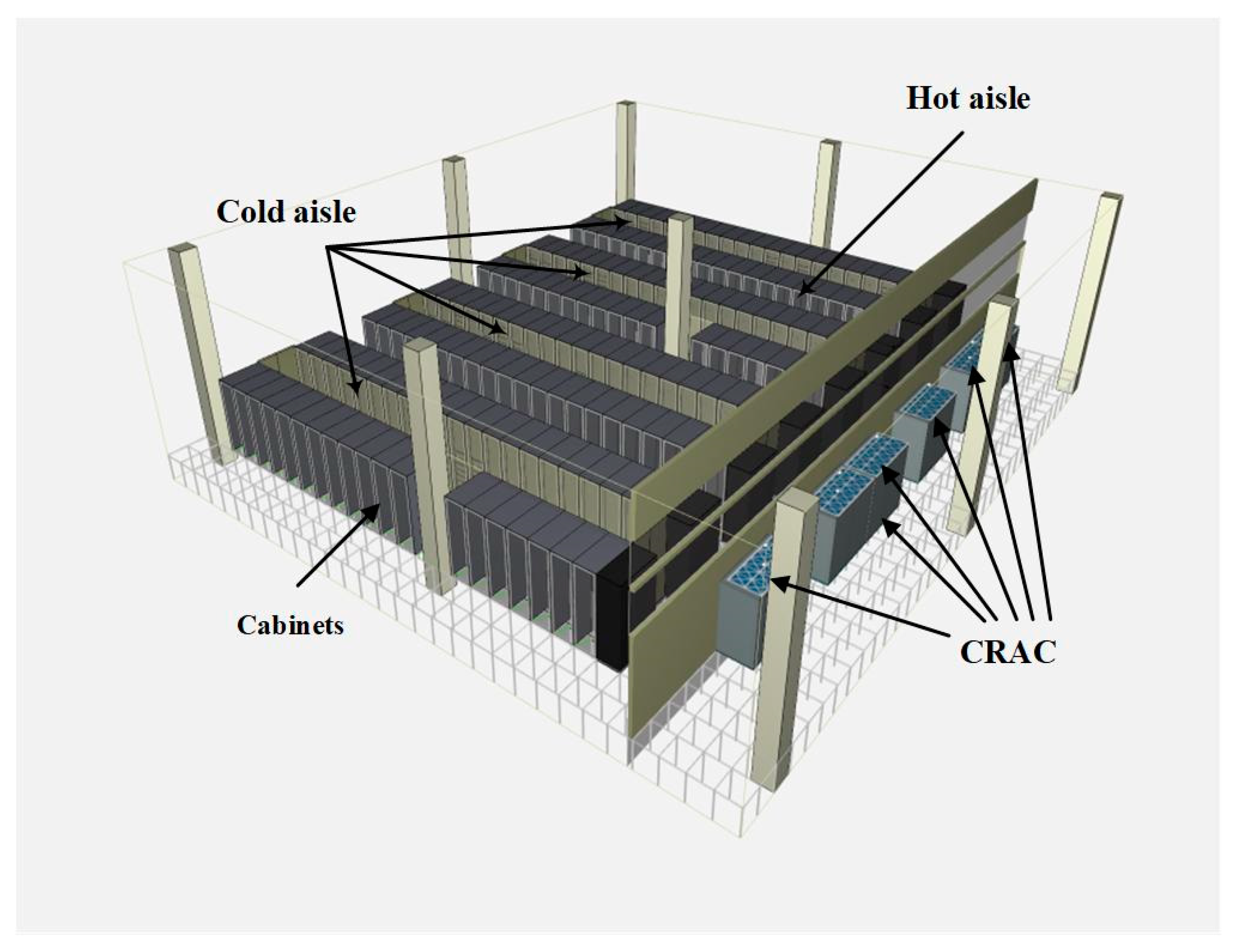
2.1. Server Room Layout and CFD Model

This study focuses on a large data center in Shanghai, with the server room model shown in Figure 2. The server room adopts a raised-floor air supply cooling system, with a raised-floor height of 0.8 m and a ceiling height of 2.8 m from the raised floor. The room contains 164 server racks, arranged in 8 rows, with 21 racks in each row. Due to the presence of load-bearing columns, the 13th and 14th racks in the 4th and 8th rows are omitted, and the gap areas are blocked off with partition walls. The server room is equipped with six computer room air conditioners (CRAC1–6), which are separated from the racks by ventilated partitions. Each pair of server racks forms a closed aisle, with perforated flooring beneath the aisle. The cold air from the CRACs flows through the floor, is expelled from the sides of the servers, and then returns to the air conditioners via the gaps above the partition. Other areas in the server room, except for the closed aisles, are designated as hot aisles. To better manage the servers, they are evenly distributed across the 2nd, 3rd, 4th, 6th, 7th, and 8th rows of racks, while the middle and one side of the room are kept idle. To ensure that the air conditioners fully cover the densely packed server areas, previous tests have shown that the optimal on/off configuration for the air conditioners is to turn on ACU2, 3, 5, and 6, while turning off the other two units. Therefore, the simulation model primarily focuses on optimizing the parameters of these four air conditioners.

2.2. Governing Equation for the CFD Model

Mathematical equations form the foundation of any numerical simulation. The flow field inside the data center investigated in this study satisfies the Bernoulli assumption. The CFD model calculates the parameters inside the computer room based on the following conservation equations.
(1)
Mass Balance Equation
The airflow follows the mass conservation equation, which states that the rate of change of the total mass within a control volume over a given time period is equal to the net mass entering the control volume during the same time interval.
ρ τ + d i v ρ v = 0
In Equation (1), ρ is the air density, in kg/m3; τ is time, in s; and v is the fluid velocity vector, in m/s.
(2)
Momentum Balance Equation
Any flow process must comply with the momentum balance equation, which asserts that the sum of all external forces acting on the control volume is equal to the rate of change of momentum of the fluid within the control volume.
ρ v x τ + d i v ρ v v x = d i v μ g r a d v x + S x
ρ v y τ + d i v ρ v v y = d i v μ g r a d v y + S y
ρ v z τ + d i v ρ v v z = d i v μ g r a d v z + S z
In Equations (2)–(4), v x , v y , and v z represent the velocity components of the fluid in the direction x, y, and z, respectively, measured in m/s; μ is the dynamic viscosity of air, in Pa·s; and S x , S y , and S z are the generalized source terms. In this simulation, the generalized source terms are all 0.
(3)
Energy Balance Equation
The energy balance equation posits that the rate of change of energy within the control volume is equal to the net energy transferred to the control volume by heat convection and conduction, along with the internal heat flux density of the control volume. The derived equation is as follows:
ρ t τ + d i v ρ v t = d i v λ c p g r a d t + R r
In Equation (5), t is the fluid temperature, in °C; λ is the thermal conductivity of air, in W/m·K; c p is the specific heat capacity of air at constant pressure, in J/kg·K; and R r is the source term.
(4)
Turbulence Model
In this study, the CFD simulation uses the standard κ ε model. This model is based on semi-empirical formulae developed by previous researchers and provides good computational accuracy and speed. The κ equation is a precise equation used to solve the turbulence kinetic energy, and the ε equation is derived from empirical formulae to solve the turbulence dissipation rate.
The κ equation is as follows:
ρ κ τ + ρ u i κ x i = μ + μ t σ κ κ x j x i + G κ ρ ε
The ε equation is as follows:
ρ ε τ + ρ u i ε x i = μ + μ t σ ε ε x j x i + C 1 ε ε κ G κ C 2 ε ρ ε 2 κ
The calculation formula for the turbulent viscosity coefficient is as follows:
μ t = ρ C μ κ 2 ε
(5)
Boundary Conditions
In our simulation, we used a fixed-temperature boundary condition to describe the temperature control of the cabinet surface. We assumed the temperature of the cabinet surface is fixed, as the goal of the precision air-conditioning system is to maintain the cabinet within a specific temperature range.
T c a b i n e t = T s e t
q c o n v = h T c a b i n e t T
where T c a b i n e t is the temperature on the cabinet surface; T s e t is the target temperature set by the air-conditioning system; q c o n v is the heat transfer rate through the cabinet surface; and T is the surrounding fluid (air) temperature.

2.3. Target Cabinet Temperature Response Control Strategy

The boundary conditions for the CRACs were set as shown in Table 1. The rated load of the cabinets inside the data center is 4 kW, but the actual average load of each cabinet is 2 kW. Each cabinet can accommodate up to 10 servers, with the server model named HP SE1120. The load of each cabinet is evenly distributed across each server. To achieve precise temperature control for the CRACs, temperature sensors were installed at the ventilation openings at half the height of the cabinets, transmitting the outlet air temperature of the cabinets to the CRAC system. In the actual data center experiment, the temperature sensors were placed at the upper, middle, and lower positions of the air inlet and outlet of each cabinet (shown in Figure 3) to obtain more detailed temperature data. The measurements show that the further a cabinet is from a CRAC, the higher the intake temperature. This indicates that the cooling effect of the CRAC system decreases as the distance from the cabinets increases.
This study used the built-in influence area calculation function for CRAC systems in 6sigmaRoom [12] to determine the influence area of each CRAC, and the results are consistent with the experimental measurements. The study applied the method of local sensitivity analysis to investigate the effects of variations in the supply air temperature of CRACs within a certain range on the cabinet temperature. The principle is to change the value of only one variable and study its singular impact on the output value. In sensitivity analysis, the parameter used to measure the degree of influence of the input variable on the output value is called the sensitivity coefficient. It can be positive or negative. A positive value indicates a positive correlation, while a negative value indicates a negative correlation. The larger the absolute value of the sensitivity coefficient, the greater the impact of that variable on the output. The formula is as follows:
S i = Δ y / y Δ x i / x i 100 %
In the formula, S i represents the sensitivity coefficient of the i th input variable, %; y denotes the model output; Δ y is the change in the model output; x i refers to the i th input variable; and Δ x i is the change in the i th input variable.
Figure 4 illustrates an example of the impact of target cabinet nodes of the CRAC system on nearby cabinets using the method described above. The impact parameter ranges from 0% to 100%, with red indicating a high impact and blue indicating a low impact. From the figure, it can be seen that the farther a cabinet is from a CRAC, the smaller the impact of the air conditioner on the cabinet.
The above method was used to analyze four active CRACs (CRAC2, CRAC3, CRAC5, and CRAC6), and the cabinets with an impact degree ≥ 50% on the CRAC system were selected as the target cabinets for each air conditioner. The sensor temperatures of each cabinet were recorded and used as the response parameters for the corresponding CRACs. In subsequent operations, the CRACs would only respond to temperature changes in the cabinets within the impact area. The specific range of the cabinets’ response to each air conditioner is shown in Figure 5.

2.4. Simulation Results

After the model parameters were set, the operating conditions of a cabinet in the data center at a specific time in the afternoon were selected as sample input for the CFD model to obtain the outlet air temperature of the CRAC system based on the target cabinet’s temperature response. In the actual data center, the outlet air temperature of the CRACs is not adjusted in real time according to the load changes of randomly selected cabinets, but set to a constant value based on historical experience. For example, the outlet air temperature of ACU2 and ACU3 is fixed at 20 °C, while that of ACU5 and ACU6 is set to 22 °C. In the CFD model, the control strategy is based on the temperature response of the target cabinet, with the target cabinet temperature set at 24 °C for the experiment.
After running the CFD simulation and stabilizing the cabinet temperatures, the presence of any local hotspots was monitored. Figure 6 shows the temperature distribution of the cabinets in the data center. It can be seen that the cabinet temperatures are within the cooling and air-conditioning engineering standard (ASHRAE 18–27 °C), confirming that the cabinets are operating in a safe temperature range. At this point, the outlet air temperature of the CRACs was recorded, and the reduced power consumption was calculated based on the CRAC model. As shown in Table 2, after adopting the control strategy based on the target cabinet temperature as a control parameter, the outlet air temperature of the CRACs was significantly higher than the set temperature based on experience. The average power reduction for the four CRACs was 0.881 kW, indicating that the experience-based control strategy for CRACs in the data center results in overcooling, and has energy-saving potential.
To verify the accuracy of the model simulation, a mesh independence analysis was conducted by incrementally increasing the grid number by 1.5 times and setting four different grid quantities. The variation in the output temperature of the target CRAC was tested as the number of grids increased, and the results are shown in Table 3. It can be seen that, with the increase in the grid number, the temperature difference in the outlet air from ACU2 did not exceed 1.2%, which demonstrates the accuracy of the simulation calculation.

3. Graph Neural Networks and Datasets

3.1. Artificial Neural Networks

An artificial neural network (ANN) is a computational model that simulates the structure and function of biological neural systems. It consists of numerous nodes connected in a hierarchical structure, typically including an input layer, hidden layers, and an output layer. Each neuron communicates and processes information with other neurons through weighted connections. Through learning algorithms, neural networks can automatically extract features from large amounts of data and perform tasks such as pattern recognition, regression prediction, and classification. Due to their powerful adaptive capabilities and nonlinear processing abilities, artificial neural networks are widely used in fields such as image recognition, speech processing, and financial forecasting.

3.2. Thermal Recirculation Phenomenon in Data Centers

In the airflow distribution inside a data center, there exists an uneven temperature distribution caused by hot air recirculation and cold air bypass. The differences in temperatures between cabinets interfere with each other [13]. The heat generated by each cabinet is not only produced by the cabinet itself, but is also influenced by the heat generated by the other five neighboring cabinets. Additionally, the airflow entering and exiting each cabinet also affects the heat distribution. Assuming each cabinet is a heat source, the thermal recirculation phenomenon can be represented as shown in Figure 7. In the figure, a i j represents the percentage of heat recirculating from the outlet of server i to the inlet of server j, and Q j represents the heat carried by the airflow passing through server j.
This phenomenon can affect the outlet air temperature of the CRACs. Therefore, location features can be incorporated to predict the cabinet outlet temperature. However, an ANN cannot consider the information of local location features or capture complex structural relationships, which may affect the accuracy of the training results. In this case, using graph neural networks (GNNs) for analysis is a better choice.

3.3. Graph Neural Networks

Graph neural networks (GNNs) are a type of deep learning models specifically designed to handle graph-structured data. In many real-world applications, data often exhibit non-Euclidean structures, with relationships that may be either close or distant. GNNs can capture the complex relationships and dependencies between nodes by directly performing computations on the graph structure, thereby effectively learning the representations of nodes, edges, and the entire graph.
A graph G = V , E is composed of nodes V and edges E . GNNs leverage the connectivity structure of the graph’s edges and vertices, as well as the attribute information related to the graph structure, to extract latent graph information.
H l + 1 = σ D ˜ 1 2 A ˜ D ˜ 1 2 H l W l
In Equation (12), H l represents the output of the l th layer network, H l R n × d ; n is the number of nodes in the graph G = V , E , with each node represented by a d -dimensional feature vector; A is the adjacency matrix of the undirected graph, where A ˜ = A   +   I N , I N is the n -dimensional identity matrix; D ˜ is the degree matrix of the undirected graph, D ˜ = j A ˜ i j ; W l R d × h are the parameters to be trained, with h being the output dimension; and σ is the activation function applied.
Graph Convolutional Network (GCN) is a variant of GNNs, and its emergence is inspired by the application of convolutional neural networks in image recognition. In simple terms, GCN aggregates the features of the neighboring nodes of each point in a graph through the adjacency matrix. With each iteration, the feature of each vertex in the graph derives more information from its surrounding vertices. This alters the feature dimensions and increases the receptive field, making the information of each vertex more comprehensive.
GCN models generally assume that all edges in the graph have the same importance, which has limitations in the context of data center applications. The Graph Attention Network (GAT), proposed in [14], addresses this by introducing multiple attention matrices to learn the importance of adjacent nodes. As shown in Figure 8, the GAT model introduces attention matrices, considering that the importance between vertices can vary. For any vertices and edges, the GAT model first introduces a learnable attention weight matrix between them, and for any nodes x i and y i , it learns the attention weight matrix α i j between these nodes.
The above figure can be expressed by a mathematical expression (2), specifically as follows:
α i j = exp LeakyReLU α W h i | | W h j k N i exp LeakyReLU α W h i | | W h j
In Equation (13), LeakyReLU is a nonlinear activation function; | | represents the concatenation of the hidden layers of nodes x i and y i , followed by normalization to obtain the attention weight matrix, which is an asymmetric matrix. This asymmetry allows the importance of nodes in the graph to be differentiated. Based on the attention weights α i j , the hidden layers of neighboring nodes h i are aggregated using a weighted average, resulting in the hidden layer of the node being h i .

3.4. Network Architecture Setup

The study combined the GCN and GAT to design a network structure for temperature prediction, as shown in Figure 9. First, the adjacency matrix and feature matrix of the input graph (①) are processed, and then the adjacency matrix and feature matrix are updated through the GCN to form (②). Next, the GAT enhances the focus on key neighbors, continuing to update the adjacency matrix and feature matrix to form (③), thereby improving the accuracy of information processing. Finally, the GCN is used again to integrate the information, maintaining both structural integrity and extensiveness, resulting in (④), which allows the model to better understand the complex structures and relationships within the graph. This process is analogous to information collection and decision-making within a team, enhancing adaptability and sensitivity to different node features. Lastly, the feature matrix in (④) is converted into a dimensional matrix, which is passed through a fully connected layer to output a one-dimensional value. The input parameters are the power of each cabinet, and the output parameter is the air outlet temperature of the CRAC.
The first layer takes the adjacency matrix and feature matrix as input, with the feature dimension set to 10. After passing through the GCN, the output dimension is 64. In the second layer, a learnable attention matrix, is introduced, and the output dimension is reduced to 32. Finally, another GCN layer is applied, reducing the output dimension to 16. Between each layer, a nonlinear activation function, RELU, is added, and a dropout parameter of 0.5 is set. In the end, a fully connected layer is used, and the output dimension is 1, representing the air outlet temperature. The specific network structure is shown in Figure 10 below.

3.5. Graph Model and Dataset

To meet the requirements of graph neural networks, the computer room was modeled by creating four graph models based on the operation of four CRAC units (ACUs) within the room. Each graph model selects the target cabinets associated with one CRAC unit as vertices. Taking the graph model composed of ACU2 as an example, as shown in Figure 11, the temperature of each cabinet in an enclosed space is most significantly influenced by the five nearest surrounding cabinets. Therefore, each cabinet is connected to its five nearest neighboring cabinets to form edges. If two cabinets are not located within the same enclosed aisle, as illustrated in the figure, the cabinets at the edges of the graph model are connected to ensure the connectivity of the graph model.
Given that the data center computer room adopts a modular design with identical spatial layouts across all rooms, it is sufficient to study the physical model of a single room. However, the distribution of servers and their load conditions within the room is not fixed. To ensure the model’s general applicability to data centers, Monte Carlo sampling (Markov Chain Monte Carlo, MCMC) was employed to randomly assign power distributions ranging from 0 kW to 4 kW to the cabinets. Generating data samples in this manner avoids deviations from real-world scenarios while ensuring good variability in cabinet loads [15]. A total of 1000 distinct combinations were generated, representing 1000 possible cases of load distribution within the computer room.
The corresponding graph models for the four CRACs are denoted as Graph 2, Graph 3, Graph 5, and Graph 6. Table 4 presents the graph feature information for these four graph models, where the feature of each vertex in the graph is represented by the corresponding load of the cabinet. Since each cabinet can accommodate 10 servers, the feature of each vertex is set as a 10-dimensional vector. From the 1st to the 10th dimension, these represent the loads of the 10 servers in the cabinet from the bottom to the top. The load is evenly distributed across all the servers in the cabinet. Therefore, for cabinets with a load between 0 and 4 kW, the vertex features are generated as a 10-dimensional matrix, as shown in Table 5.
Figure 12 presents a set of random sample load cases, where the load range of each server is from 0 to 400 W. A total of 1000 load cases were used to form 4000 datasets, with 95.8% selected as the training set and 4.2% as the test set, which were then input into the GNNs for training and testing. The same data were also input into the ANN for the prediction of outlet temperature. Finally, we used mean squared error (MSE) to compare the accuracy of the ANN and GNNs. The formula for MSE is as follows:
M S E = 1 n i = 1 n y i y ^ i 2
where n is the number of the samples, y i represents the actual value, and y ^ i represents the predicted value.
In the ANN, the network layers directly take the cabinet load (1D) within the target cabinet area as input, with the output dimensions being the same as those of the GNNs. The hidden layers consist of two layers, with dimensions of 64 and 32, respectively, and a dropout rate of 0.5.

4. Results

The results of the test set were analyzed in this experiment. ACU2, ACU3, ACU5, and ACU6 in the experiment correspond to the graph models, specifically Graph 2, Graph 3, Graph 4, and Graph 5, respectively. Based on the mean squared error (MSE) of each group of data in Table 6, it can be observed that, in terms of prediction accuracy, Graph 2 and Graph 3 outperform Graph 4 and Graph 5. This is because Graph 4 and Graph 5 have a larger span compared to the first two graph models. For larger and irregularly shaped graph models, the internal relationship between vertices and edges can be further optimized. However, when comparing the training results of the designed network with those of a conventional ANN, it is evident that the results from the designed network are far superior to those from the ANN. This is because the ANN model does not account for the direct interactions between the input data, and its relatively simple network layers contribute to the lower performance.
Figure 13 shows the relationship between the predicted results of the four graph models and the simulation results. It is evident that the predicted temperatures for ACU2 and ACU3 are generally higher than the empirically set temperature of 20 °C, and those of ACU5 and ACU6 are generally higher than the empirically set temperature of 22 °C. The overall deviation between the predicted and simulation values is within the allowable error of ±0.5 °C for CRACs in data centers. Although there are some individual data points with significant deviations, they do not affect the overall performance.
Figure 14 visualizes the deviation between the predicted and simulation values for the 168 test set data points. As shown in the figure, 161 data points exhibit a difference ≤ ±0.5 between the predicted and target values, accounting for 95.83% of all predictions, while 7 data points display a deviation greater than 0.5. Generally, an error of CRACs in data centers within ±0.5 °C is considered normal [16]. Therefore, the model’s prediction of the air outlet temperature for the CRACs meets the accuracy requirements.

5. Conclusions

This study has proposed a CRAC control strategy based on the working temperature response of target cabinets, aiming to optimize the temperature control performance of air-conditioning systems in data centers. The implementation of this strategy leads to significant energy savings; specifically, the average power reduction for the four air-conditioning units was 0.881 kW, demonstrating the effectiveness of the proposed control strategy in reducing energy consumption compared to traditional experience-based cooling methods. This result indicates that the strategy helps to optimize the cooling system’s energy efficiency while preventing overcooling, which is a common issue in data centers. Furthermore, the accuracy of the proposed model was validated by comparing its performance to that of traditional methods. The graph neural network (GNN) model outperformed the artificial neural network (ANN) model in terms of predicting outlet air temperatures. For instance, the GNN model achieved mean squared error (MSE) values of 0.02305 for Graph 2 and 0.0366 for Graph 3, which were significantly lower than those (0.2675 and 0.2372, respectively) observed for the ANN model. This highlights the superior accuracy and robustness of the GNN model in predicting outlet air temperature for CRAC units.
The performance of the proposed model was further validated using a test set. The results show that 95.83% of the predictions displayed a deviation within ±0.5 °C, which is well within the acceptable error margin for CRAC systems, thus meeting ASHRAE standards. Only 7 data points out of the total 168 test points showed deviations greater than ±0.5 °C, demonstrating the high accuracy of the model. These results confirm that the proposed strategy meets the required accuracy for real-world applications in data centers. Additionally, CFD-based simulations confirmed that dynamic adjustments to supply air temperature based on real-time server room loads and equipment requirements significantly reduce localized hotspots and optimize overall cooling efficiency. This dynamic regulation strategy enables more flexible and intelligent control of air-conditioning systems, improving energy conservation and reducing manual intervention. The results highlight the potential of this approach to enhance both the operational efficiency and reliability of CRAC systems in data centers.

Author Contributions

Conceptualization, Q.S.; methodology, Q.S.; software, Q.S.; validation, Q.S. and J.Y.; formal analysis, Q.S.; investigation, Q.S.; resources, Q.S.; data curation, Q.S.; writing—original draft preparation, Q.S.; writing—review and editing, Q.S. and J.Y.; visualization, Q.S.; supervision, J.Y., R.S. and Y.W.; project administration, J.Y. and R.S.; funding acquisition, Y.W. All authors have read and agreed to the published version of the manuscript.

Funding

This research was funded by the National Natural Science Foundation of China (NSFC), grant number 51806096.

Data Availability Statement

The original contributions presented in the study are included in the article, further inquiries can be directed to the corresponding author.

Conflicts of Interest

The authors declare no conflicts of interest.

References

  1. Jones, N. The information factories. Nature 2018, 561, 163–166. [Google Scholar] [CrossRef] [PubMed]
  2. Kleyko, D.; Osipov, E.; Patil, S.; Vyatkin, V.; Pang, Z. On methodology of implementing distributed function block applications using TinyOS WSN nodes. In Proceedings of the 2014 IEEE Emerging Technology and Factory Automation (ETFA), Barcelona, Spain, 16–19 September 2014; pp. 1–7. [Google Scholar] [CrossRef]
  3. Zhou, H.; Li, Z.; Liu, Y.; Mei, L.; Lu, W.; Hu, J.; Cai, D. Air Conditioning System Design of Power Data Center Based on Automatic Control Technology. In Proceedings of the 2024 IEEE 2nd International Conference on Image Processing and Computer Applications (ICIPCA), Shenyang, China, 28–30 June 2024; pp. 1–4. [Google Scholar] [CrossRef]
  4. Ahmad, M.W.; Mourshed, M.; Yuce, B.; Rezgui, Y. Computational intelligence techniques for HVAC systems: A review. Build. Simul. 2016, 9, 359–398. [Google Scholar] [CrossRef]
  5. Wu, Y.; Xue, X.; Le, L.; Ai, X.; Fang, J. Real-time Energy Management of Large-scale Data Centers: A Model Predictive Control Approach. In Proceedings of the 2020 IEEE Sustainable Power and Energy Conference (iSPEC), Chengdu, China, 23–25 November 2020; pp. 2695–2701. [Google Scholar] [CrossRef]
  6. Kwon, Y.I. A study on the evaluation of ventilation system suitable for outside air cooling applied in large data center for energy conservation. J. Mech. Sci. Technol. 2016, 30, 2319–2324. [Google Scholar] [CrossRef]
  7. Yi, Y.; Zheng, A.; Shao, X.; Cui, G.; Wu, G.; Tong, G.; Gao, C. Joint Adjustment of Emergency Demand Response Considering Data Center and Air-Conditioning Load. In Proceedings of the 2018 IEEE International Conference on Energy Internet (ICEI), Beijing, China, 21–25 May 2018; pp. 72–76. [Google Scholar] [CrossRef]
  8. Su, Z. Optimization of an IDC Center Cooling System Based on PUE Analysis. Refrig. Air Cond. 2021, 35, 162–168. [Google Scholar]
  9. Ni, J.; Liu, S.Y.; Yuan, Z.Y.; Zhang, W.Q.; Gao, B. Optimization of Cooling System Performance of a Data Center in Sichuan Province. Refrig. Air Cond. 2023, 37, 410–416. [Google Scholar]
  10. Nada, S.A.; Said, M.A. Effect of CRAC units layout on thermal management of data center. Appl. Therm. Eng. 2017, 118, 339–344. [Google Scholar] [CrossRef]
  11. Available online: https://www.cadence.com/en_US/home/tools/reality-digital-twin.html#cadence-reality-dc-design (accessed on 14 September 2024).
  12. Tang, Q.; Gupta, S.K.S.; Stanzione, D.; Cayton, P. Thermal-Aware Task Scheduling to Minimize Energy Usage of Blade Server Based Datacenters. In Proceedings of the 2006 2nd IEEE International Symposium on Dependable, Autonomic and Secure Computing, Indianapolis, IN, USA, 29 September 2006–1 October 2006; pp. 195–202. [Google Scholar] [CrossRef]
  13. Montgomery, D.C. Design and Analysis of Experiments; John Wiley & Sons: Hoboken, NJ, USA, 2017; Available online: https://www.wiley.com/en-us/Design+and+Analysis+of+Experiments%2C+10th+Edition-p-9781119492443 (accessed on 14 September 2024).
  14. Veličković, P.; Cucurull, G.; Casanova, A.; Romero, A.; Lio, P.; Bengio, Y. Graph Attention Networks. arXiv 2018, arXiv:1710.10903. [Google Scholar]
  15. Athavale, J.; Joshi, Y.; Yoda, M. Artificial Neural Network Based Prediction of Temperature and Flow Profile in Data Centers. In Proceedings of the 2018 17th IEEE Intersociety Conference on Thermal and Thermomechanical Phenomena in Electronic Systems (ITherm), San Diego, CA, USA, 29 May 2018–1 June 2018; pp. 871–880. [Google Scholar] [CrossRef]
  16. ASHRAE Standard 90.1-2016; Energy Standard for Buildings Except Low-Rise Residential Buildings. ASHRAE: Peachtree Corners, GA, USA, 2016.
Figure 1. Technical approach.
Energies 18 01803 g001
Figure 2. Data center model.
Energies 18 01803 g002
Figure 3. Position of the temperature sensors.
Energies 18 01803 g003
Figure 4. The CRACs’ influence area.
Energies 18 01803 g004
Figure 5. The target racks of each CRAC.
Energies 18 01803 g005
Figure 6. Simulation results regarding temperature compliance.
Energies 18 01803 g006
Figure 7. Schematic diagram of the thermal cycle in a data center.
Energies 18 01803 g007
Figure 8. Illustration of GAT model.
Energies 18 01803 g008
Figure 9. Schematic diagram of the deep learning-based prediction.
Energies 18 01803 g009
Figure 10. Algorithm flowchart.
Energies 18 01803 g010
Figure 11. Schematic diagrams of graph structures for graph model 2.
Energies 18 01803 g011
Figure 12. Sample of the data center operating conditions.
Energies 18 01803 g012
Figure 13. Test set prediction outcomes for the four images.
Energies 18 01803 g013
Figure 14. Summary of deviation values.
Energies 18 01803 g014
Table 1. Boundary conditions for CRACs.
CRAC Settings
Cooling MethodChilled Water Cooling
Fan Speed70%
Outlet Temperature Range13~25 °C
Rated Power Consumption8.1 kW
Maximum Sensible Cooling Capacity145 kW
Rated Airflow37,500 m3/h
Table 2. Comparison of temperatures in CRACs with two strategies.
Air Conditioner’s IDEmpirically Set Temperature (°C)Experimentally Measured Temperature (°C)Power Reduction (kW)
ACU1stoppedstopped/
ACU22024.41.782
ACU32021.90.770
ACU4stoppedstopped/
ACU52223.10.446
ACU62223.30.527
Table 3. Mesh independence analysis.
MeshCell NumbersTemperature of ACU2
(°C)
Percentage Difference
(%)
Mesh-160630224.3971/
Mesh-277078424.52660.531
Mesh-3103011824.63210.430
Mesh-4162154024.92781.200
Table 4. Information on graph features.
Figure IDGraph 2Graph 3Graph 5Graph 6
Number of Nodes33405442
Number of Edges6392128101
Feature of EdgeUndirectedUndirectedUndirectedUndirected
Number of Features330440540420
Label Rate100%100%100%100%
edge_index[2,126][2,184][2,236][2,202]
Table 5. The characteristic matrix for a cabinet with a power consumption of x W.
Power xDescription of Feature Matrix
400[x/2, x/2, 0, 0, 0, 0, 0, 0, 0, 0]
400~800[x/4, x/4, x/4, x/4,0,0,0,0,0,0]
800~1200[x/6, x/6, x/6, x/6, x/6, x/6, x/6,0,0,0,0]
1200~1600[x/8, x/8, x/8, x/8, x/8, x/8, x/8, x/8,0,0]
1600~2000[x/10, x/10, x/10, x/10, x/10, x/10, x/10, x/10, x/10, x/10]
2000~2400[x/10, x/10, x/10, x/10, x/10, x/10, x/10, x/10, x/10, x/10]
2400~2800[x/10, x/10, x/10, x/10, x/10, x/10, x/10, x/10, x/10, x/10]
2800~3200[x/10, x/10, x/10, x/10, x/10, x/10, x/10, x/10, x/10, x/10]
3200~3600[x/10, x/10, x/10, x/10, x/10, x/10, x/10, x/10, x/10, x/10]
3600~4000[x/10, x/10, x/10, x/10, x/10, x/10, x/10, x/10, x/10, x/10]
Table 6. MSE of each graph model.
Figure IDGraph 2Graph 3Graph 5Graph 6
GNNs0.023050.03660.19680.1301
ANN0.26750.23720.62110.4070
Disclaimer/Publisher’s Note: The statements, opinions and data contained in all publications are solely those of the individual author(s) and contributor(s) and not of MDPI and/or the editor(s). MDPI and/or the editor(s) disclaim responsibility for any injury to people or property resulting from any ideas, methods, instructions or products referred to in the content.

