Research on Wind Power Grid Integration Power Fluctuation Smoothing Control Strategy Based on Energy Storage Battery Health Prediction

Abstract

Due to the volatility and uncertainty of wind power generation, energy storage can help mitigate the fluctuations in wind power grid integration. During its use, the health of the energy storage system, defined as the ratio of the current available capacity to the initial capacity, deteriorates, leading to a reduction in the available margin for power fluctuation smoothing. Therefore, it is necessary to predict the state of health (SOH) and adjust its charge/discharge control strategy based on the predicted SOH results. This study first adopts a Genetic Algorithm-Optimized Support Vector Regression (GA-SVR) model to predict the SOH of the energy storage system. Secondly, based on the health prediction results, a control strategy based on the model predictive control (MPC) algorithm is proposed to manage the energy storage system’s charge/discharge process, ensuring that the power meets grid integration requirements while minimizing energy storage lifespan loss. Further, since the lifespan loss caused by smoothing the same fluctuation differs at different health levels, a fuzzy adaptive control strategy is used to adjust the parameters of the MPC algorithm’s objective function under varying health conditions, thereby optimizing energy storage power and achieving the smooth control of the wind farm grid integration power at different energy storage health levels. Finally, a simulation is conducted in MATLAB for a 50 MW wind farm grid integration system, with experimental parameters adjusted accordingly. The experimental results show that the GA-SVR algorithm can accurately predict the health of the energy storage system, and the MPC-based control strategy derived from health predictions can improve grid power stability while adaptively adjusting energy storage output according to different health levels.

1. Introduction

Climate change has become a central global issue, with the development of clean energy and the reduction of carbon emissions emerging as crucial strategies to combat global warming and the increasing frequency of extreme weather events. Around the world, countries are making significant strides in building green power generation infrastructure, such as wind, hydro, and nuclear energy, to address environmental, climate, and ecological challenges [1,2]. In this context, lithium-ion battery energy storage systems, as a cutting-edge clean energy solution, have become integral to the integration of renewable energy sources into the grid. With their notable advantages, such as their safety, high energy density, and long operational life, these systems are key to mitigating power fluctuations, balancing grid loads, smoothing peak–valley variations, and stabilizing both grid frequency and voltage [3,4,5].

The SOH of a lithium-ion battery is how much usable power it has now compared to when it was new, which directly demonstrates its capabilities to smooth wind power variations. This smoothing capability ensures the stability of wind power grid integration. Improving the accuracy of lithium-ion battery health prediction can not only guarantee safety but also enhance energy efficiency and extend its lifespan [6]. As a result, predicting the health of lithium-ion batteries has been a major focus of research. However, accurately estimating the health state of these batteries remains challenging due to their complex physical and chemical reactions. Currently, methods for predicting the health of lithium-ion batteries are typically classified into four categories [7]: electrochemical model-based methods, experimental-based methods, physics-based methods, and data-driven methods.

Electrochemical model-based methods [8,9,10] are highly accurate, as they rely on electrochemical reaction processes and aging mechanisms such as migration, diffusion, and chemical reaction kinetics. However, these models need a lot of different equations, which makes them expensive to run on computers, making them less commonly employed. Experimental-based methods [11] predict health by deriving mathematical expressions for battery capacity degradation through fitting. While this approach is computationally efficient, the mathematical expressions may not always align with actual charging and discharging conditions, so their accuracy remains uncertain. Physics-based methods [12,13,14] involve constructing equivalent circuit models, such as RC and PNGV models, and using the relationships between battery parameters (e.g., capacity and resistance) for capacity prediction, which is then used to estimate the state of health. However, these methods also have drawbacks, such as the need for complex matrix calculations and the complication of capacity degradation curves due to the regeneration of capacity in a stationary state [8]. In data-driven methods, some researchers use existing battery data, such as the charge/discharge depth, temperature, and charge/discharge time, to predict battery health. These methods do not require a deep understanding of the design, material properties, or physical models of different electrochemical batteries, allowing researchers to use aging data, including current, voltage, temperature, discharge amount, and charge/discharge time [15], to predict battery health. This approach does not require detailed knowledge of electrochemical battery designs or material properties. The most commonly used models in this approach are capacity loss models [16] and resistance models [17]. Furthermore, intelligent algorithms and machine learning techniques [18], such as the Genetic Algorithm (GA), Support Vector Regression (SVR), and neural networks, have also been employed to predict the battery’s SOH. These data-driven methods are particularly appealing to many researchers due to their flexibility and the fact that they do not require replicating physical models. In the prediction of battery SOH, SVR has been widely adopted as an effective forecasting method due to its strong nonlinear mapping capability and excellent generalization performance in various prediction tasks. However, practical applications of SVR still face several challenges, particularly in parameter selection. Traditional SVR approaches typically rely on manual parameter tuning, which not only requires empirical expertise but may also lead to performance fluctuations and reduced prediction accuracy. To address these limitations, this paper proposes a GA-optimized SVR parameter selection method. By leveraging the GA to automatically search and optimize critical SVR parameters, this approach enhances prediction accuracy while minimizing manual intervention, thereby improving the overall reliability and precision of battery SOH predictions.

The goal of this study is to use data-driven methods to learn the causal relationship between various aging factors and the degradation of the state of health at each time interval through algorithms. The results show that the proposed GA-SVR method successfully predicts the SOH of the energy storage (ES) system. With strong applicability, this method can be further applied to SOH prediction in real-world operational scenarios.

The grid-connected power of a wind-storage system consists of both wind power and the charge/discharge power of the energy storage system. Given the current wind power, the charge/discharge power of the energy storage system can be calculated and determined by setting a target grid-connected power. In the use of energy storage to smooth wind power fluctuations, some scholars have adopted filtering algorithms, wavelet packet decomposition, and empirical mode decomposition (EMD) to calculate the target power for energy storage and grid-connected power [19,20,21,22,23,24]. For example, in the literature [20], a wavelet packet decomposition algorithm is used to decompose photovoltaic (PV) power. To address the challenge of determining the parameters of wavelet packet decomposition, the author employed a filtering method to smooth out the fluctuations. However, this method also has issues with confirming the time constant and the presence of delays. In the literature [21,22], EMD and CEEMD, combined with other optimization algorithms, were used to process wind power, achieving good results. However, the drawback of their decomposition algorithms is modal aliasing, which was solved by the use of VMD [23]. In the literature [24], an adaptive variational mode decomposition algorithm was used to determine the pre-scheduling power of the wind-storage system with the goal of minimizing the overall cost. However, VMD has problems when it comes to choosing the number of modes and penalty coefficients by hand. If the mode number is set too high or too low, it can cause repeated data, adding noise or losing important information. The enhanced salp swarm algorithm (ISSA) assists in automatically determining the optimal number of layers and penalty coefficients for VMD, although it occasionally converges on a suboptimal solution.

MPC has some benefits compared to filtering control and other flexible control methods, especially when it comes to how quickly it responds and how accurate it is [25]. It can assume future control needs and make improvements [26,27]. Additionally, it makes sure that the system works well and safely by putting limits on what inputs and outputs can be.

The Literature Summary Table is summarized as follows:

In the aspect of SOH prediction:

Reference	Methodology	Advantages	Limitations
[8,9,10]	Electrochemical Model-Based Methods	High accuracy, considers electrochemical reactions	High computational cost, complex equations
[11]	Experimental-Based Methods	Computationally efficient, mathematical expression fitting	Accuracy depends on fitting equations, may not reflect real conditions
[12,13,14]	Physics-Based Methods (RC, PNGV models)	Uses real battery parameters for capacity prediction	Requires complex matrix calculations, capacity regeneration effect
[15]	Data-Driven Methods (Charge/Discharge data)	No need for deep electrochemical knowledge, flexible	Dependent on data quality, may not capture all degradation mechanisms
[16,17]	Capacity Loss and Resistance Models	Simple and widely used for SOH estimation	Limited accuracy in dynamic conditions
[18]	Machine Learning (GA, SVR, Neural Networks)	Strong generalization ability, flexible, automatic parameter tuning possible	Requires large dataset for training, sensitive to hyperparameters

In the aspect of wind power fluctuation smoothing methods:

Reference	Methodology	Advantages	Limitations
[19]	Filtering Algorithms	Simple implementation, effective in reducing high-frequency components	May cause delays, requires careful parameter tuning
[20]	Wavelet Packet Decomposition	Good for decomposing power fluctuations	Issues with selecting wavelet packet settings, potential time delays
[21,22]	Empirical Mode Decomposition (EMD, CEEMD)	Effective for wind power smoothing	Modal aliasing issue, requires optimization
[23]	Variational Mode Decomposition (VMD)	Addresses modal aliasing, improved signal decomposition	Manual selection of mode numbers and penalty coefficients
[24]	Adaptive Variational Mode Decomposition with ISSA	Optimized VMD parameter selection	May converge to suboptimal solutions

This study aims to predict the SOH of energy storage and adjust the control strategy to smooth the power fluctuations of wind energy based on different SOH conditions. The main contributions of this paper are as follows:

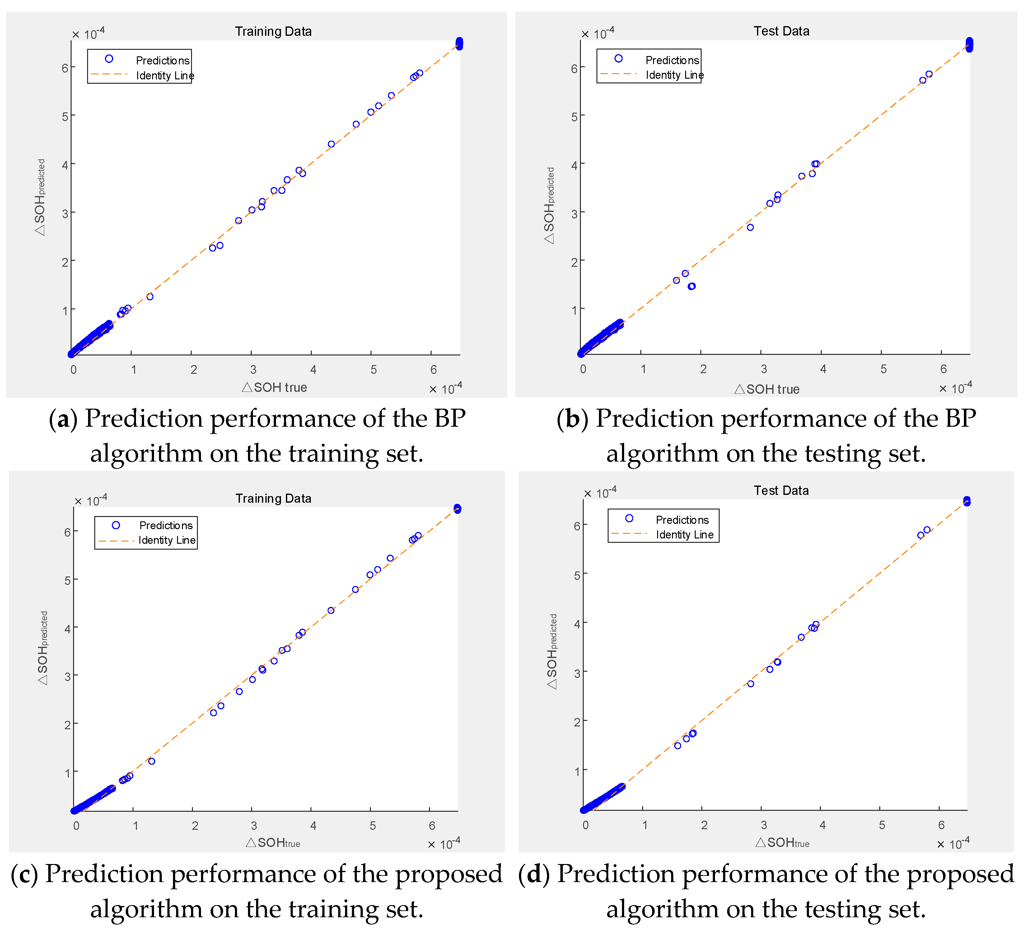
• A GA-optimized SVR algorithm is proposed to predict the SOH of the energy storage system. The proposed algorithm improves the accuracy of the energy storage health prediction results.
• A new method using MPC is suggested to manage how energy is charged and discharged in an energy storage system. This method ensures that the energy output from the storage system is reduced while still meeting the needs of the power grid, which helps to extend the life of the energy storage system.

Additionally, a fuzzy control strategy is added to enhance the MPC. This new strategy considers the SOH of the energy storage system and the changes in wind power as its inputs. It gives a weight to the objective function in the MPC, helping to adjust the control settings. This allows for balancing between smoothing out wind power changes and the output from the energy storage system. The goal is to meet the power fluctuations required by the grid while optimizing performance: when fluctuations are high, smoothing out the changes is more important; when the fluctuation is low, the energy storage output reduction is prioritized to minimize lifespan degradation. On the other hand, as a deterioration in energy storage health reduces the charge/discharge capabilities, the proposed fuzzy control strategy adaptively adjusts the parameters of the MPC objective function based on the energy storage SOH, thus controlling the energy storage output.

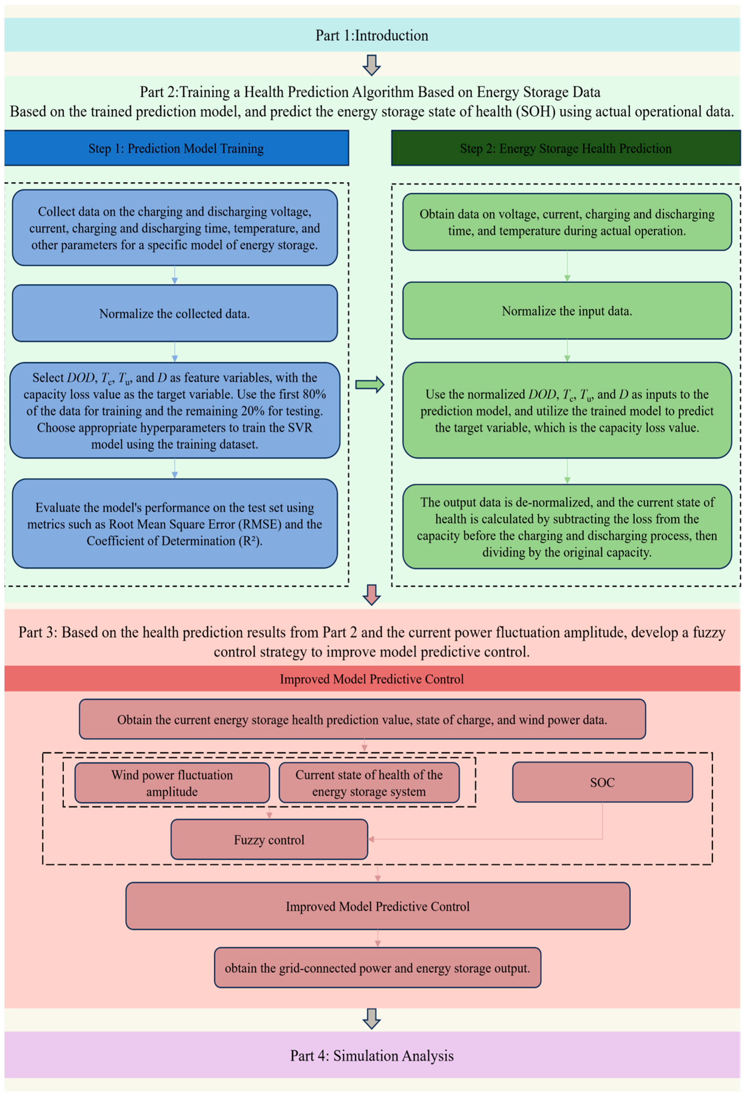
The rest of the paper is organized as follows: Section 2 explains the SOH prediction methods. This explanation, includes factors influencing energy storage lifespan, as well as machine learning regression models, and their application in predicting energy storage health. Section 3 introduces the MPC-based energy storage control strategy and the fuzzy control improvement applied to the MPC. This improvement adjusts the weight coefficients of the objective function based on energy storage SOH predictions and wind power fluctuation amplitude. Section 4 provides a simulation analysis of the wind power smoothing effect and the adjustment of energy storage output under different SOH conditions using the proposed control strategy. The paper is concluded in Section 5. Figure 1 shows the organization of this paper.

2. Calculation Method for Energy Storage SOH and Algorithm-Based SOH Prediction

2.1. Theoretical Basis of Energy Storage SOH

The SOH is typically calculated using internal resistance (SOH_R) and the remaining usable capacity (SOH_C). The first one shows how the internal resistance of a used battery compares to a new one. It tends to increase with battery usage over time. For simplicity, this study focuses on the SOH_C and collectively refers to it as the SOH.

The SOH is defined as the ratio of the current usable capacity of the battery C(t) to the initial capacity of a new battery [28], which is referred to as the nominal capacity of the battery and denoted by C_nom. This ratio can be written as follows:

$$SOH(t)=SOH(t)={\displaystyle \frac{C(t)}{C_{nom}}}$$

(1)

where C(t) can be obtained by integrating the product of the discharge voltage and the current of a complete discharge process of the battery at time t along the time axis. Studies show that the battery capacity degrades during the operational cycle, and the battery’s lifespan is considered to have ended when the capacity decreases to 80% of the rated value.

Battery capacity degradation is the cumulative result of both cycle aging and calendar aging. Research indicates that battery cycle aging is influenced by factors such as the depth of discharge, cycle count, discharge rate, and temperature, and is also related to the battery’s current state of charge and degree of aging [29].

2.2. Prediction of Energy Storage SOH Using GA-Optimized SVR

A data-driven approach is used where inputs such as the cumulative time (D), temperature (T_u), charge/discharge time (T_c), and the depth of discharge (DOD) are used to forecast SOH. The output represents the reduction in available capacity, and the SOH is calculated as the ratio of this reduction to the initial capacity. The data are split into training and testing sets for model validation.

2.2.1. Theory of SVR

Support Vector Regression (SVR) is a regression method based on support vector machines (SVMs). It effectively handles nonlinear relationships through the epsilon-insensitive loss function and kernel trick, while avoiding overfitting via regularization. SVR performs well in high-dimensional spaces and is applicable to various regression tasks. However, it exhibits significant computational overhead, sensitivity to hyperparameters, and high memory demands. Specifically, its performance heavily depends on hyperparameter combinations (regularization coefficient C, the epsilon-insensitive zone, and kernel function parameter $K\left(x_i, x_j\right)$), necessitating optimization strategies like a grid search to determine optimal configurations. Additionally, the implicit high-dimensional mapping induced by kernel functions reduces interpretability compared to parametric models such as linear regression. Nevertheless, SVR remains a powerful and flexible regression tool, particularly suited for addressing complex nonlinear problems.

SVR applies a support vector machine (SVM) for regression to predict continuous values. It minimizes model complexity while constructing an ε-insensitive tube, with the algorithm involving three parameters:

C controls the penalty for errors.

σ determines the influence of each data point.

ɛ controls the permissible error range.

SVR solves an optimization problem to find a regression function using the formula:

$$R(f)={\min }_{v,b,\xi ,{\xi }^{*}}{\displaystyle \frac{1}{2}}{‖v‖}^2+C{\displaystyle {\sum }_{i=1}^n({\xi }_i+{\xi }_i^{*})}$$

(2)

In this equation, R(f) represents the objective function to be minimized.

Constraint conditions:

$$\begin{array}{l}{y}_i-(\mathrm{v}*x_i+b)\le \epsilon +{\xi }_i\\ (v*x_i+b)-y_i\le \epsilon +{\xi }_i^{*}\\ {\xi }_i,{\xi }_i^{*}\ge 0,i=1,\dots ,n\end{array}$$

(3)

In Equations (2) and (3), v is the weight vector, $b$ is the bias, ${\xi }_i$ and ${\xi }_i^{*}$ are the slack variables, which allow some data points to lie outside the error margin ϵ, C is the regularization parameter, with C > 0 representing the penalty for samples with errors exceeding ɛ, and it is used to balance the complexity of the model and the size of the error; n is the number of training data samples. By adding slack variables ${\xi }_i$ and ${\xi }_i^{*}$, SVR lets some data points fall outside the error limit ɛ. However, the number of these points and how far they are from the limit is controlled by the regularization parameter C to avoid overfitting.

Finally, by solving this optimization problem, we can obtain the parameters v and b of the regression model, thereby obtaining the regression function:

$$f(x)=v\times x+b$$

(4)

The above is the formula expression for linear SVR. If a kernel function (such as a Gaussian kernel, a polynomial kernel, etc.) is used, it can be extended to nonlinear SVR. By using the kernel function $K\left(x_i, x_j\right)$, the nonlinear regression function is obtained as:

$$\begin{array}{l}f(x)={\displaystyle {\sum }_{i=1}^n({\alpha }_i-{\alpha }_i^{*})}K(x_i,x_j)+b\\ {\alpha }_i,{\alpha }_i^{*}\in \left[0,C\right]\end{array}$$

(5)

In the equation, ${\alpha }_i$ and ${\alpha }_i^{*}$ are the Lagrange multipliers. SVR can find a nonlinear decision function in a high-dimensional feature space, thereby modeling the complex battery aging mechanism through nonlinear mapping.

2.2.2. Genetic Algorithm-Optimized SVR

The selection of suboptimal SVR parameters may induce model overfitting, compromising the generalizability of regression models. To address this challenge, the proposed GA-SVR hybrid methodology incorporates an evolutionary-based optimization mechanism that dynamically refines these hyperparameters.

As shown in Figure 2, the GA framework for the optimization of SVR parameters is as follows:

• Decoding chromosomes: The SVR parameters C, σ, and ϵ are directly encoded to form the chromosomes.
• Create an initial group of chromosomes: The ranges for C, σ, and ϵ are set as [0, 1], [1, 100], and [0.0001, 0.01], respectively. A random group of 20 initial chromosomes is created to represent the values of the SVR parameters.
• Evaluate fitness: Leave-One-Out Cross Validation (LOOCV) is used to find the optimal values of these parameters. LOOCV is employed to evaluate fitness. In this study, the fitness function is used for this evaluation, where the actual values and predicted values represent the true outputs and the model’s predicted outputs in the training data, respectively.
• Genetic Algorithm steps: In these steps, we use a method called the roulette wheel to pick the best chromosomes to reproduce. We randomly use a single-point crossover to swap genes between two chromosomes, with a 50% chance of creating new chromosomes from each pair. Mutation happens after the crossover step to determine if a chromosome in the next generation will change. Each chromosome has a 2% chance of being mutated.
• Termination condition judgment: If the termination condition is satisfied, the GA ends and outputs the best values of C, σ, and ϵ based on the best fitness function value. Otherwise, steps 3–4 are repeated until C, σ and ϵ reach the minimum model error.

2.2.3. Steps of Energy Storage SOH Prediction Model

The GA-SVR-based SOH prediction system follows these steps:

Step 1: Data Collection and Preparation

Collect and normalize data for features like DOD, T_c, T_u, D, and capacity loss.

Step 2: Feature Engineering

Select key features and target variables for model training.

Step 3: Data Splitting

Split the dataset into 80% for training and 20% for testing.

Step 4: Model Training

Train the SVR model with selected hyperparameters.

Step 5: Model Evaluation

Evaluate the model using RMSE and R², where a smaller RMSE and a higher R² indicate better performance.

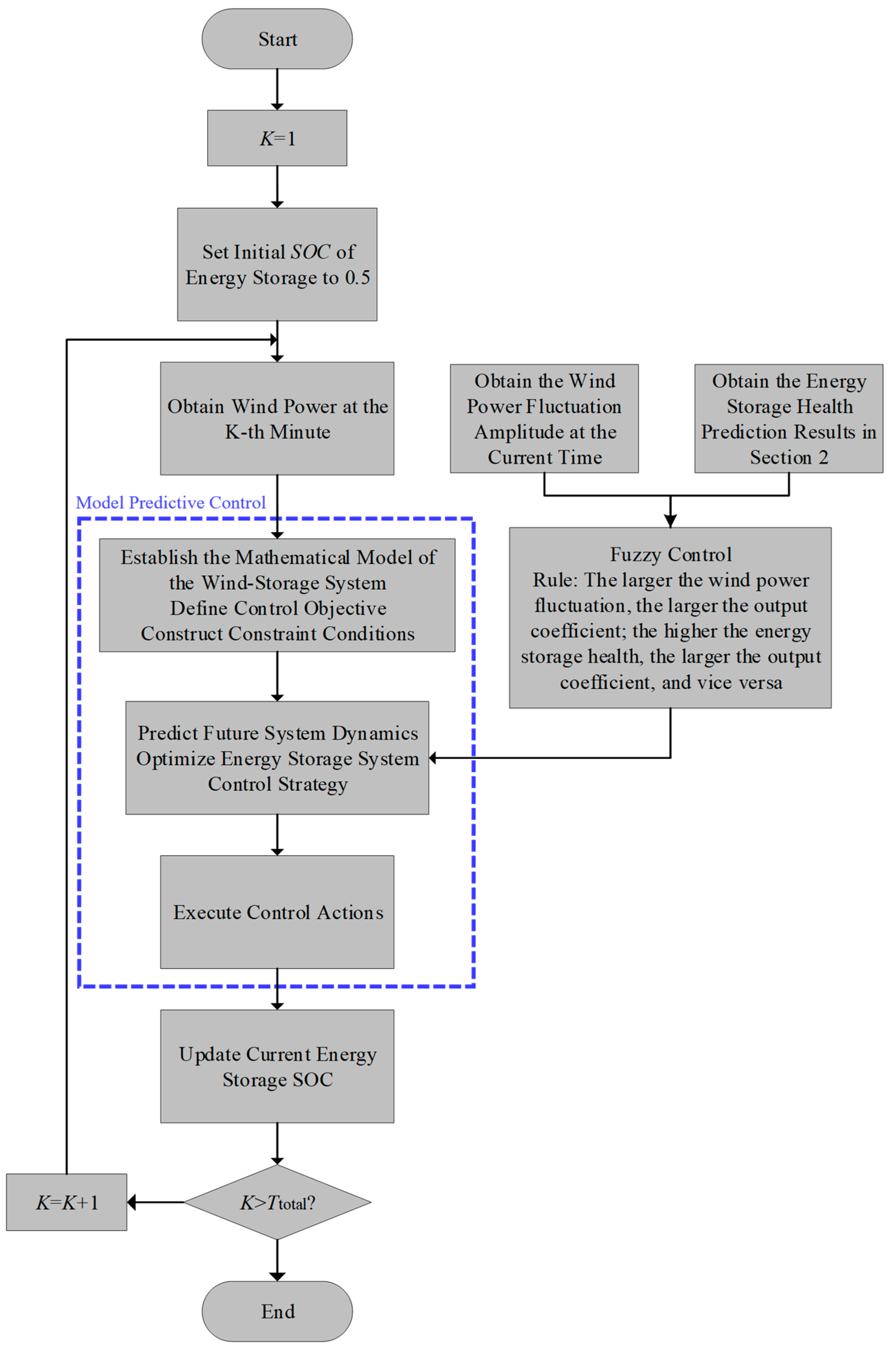
3. Improved MPC Algorithm-Based Wind Power Grid-Connected Power Fluctuation Smoothing Strategy

In Section 2, the SOH of the energy storage system is predicted. Using the expected SOH results and fuzzy control rules, an improved MPC is used to manage the energy output and reduce changes in the grid-connected power of wind power. Figure 3 depicts the control flowchart, where the energy storage SOH is referenced in Section 2.2.

Figure 3 illustrates the step-by-step process of the better control model that uses energy storage health predictions and fuzzy control rules. As seen in Figure 3, the process will keep repeating, slowly making predictions and improvements until it reaches a total time of 600 min.

As seen in Figure 3, the process will keep repeating, slowly making predictions and improvements until it reaches a total time of 600 min. In applying MPC, assume that the current control time node is K (in minutes), and the total optimization control duration T = 600 min. The optimization process can be described as follows:

Step 1: Initialization. Set the starting time node K = 1.

Step 2: At every moment K, by assessing the present circumstances, the state of the system in the future is anticipated and the control input is optimized to minimize the objective function.

Step 3: Control input update. The obtained control input is applied at the time node K based on the optimization results.

Step 4: Time node update. After the application of the control input, the time node is updated as K = K + 1.

Loop: Repeat steps 2–4 until the time node K reaches the total duration T_total = 600 min.

3.1. Model Predictive Control Algorithm for Energy Storage Power Optimization

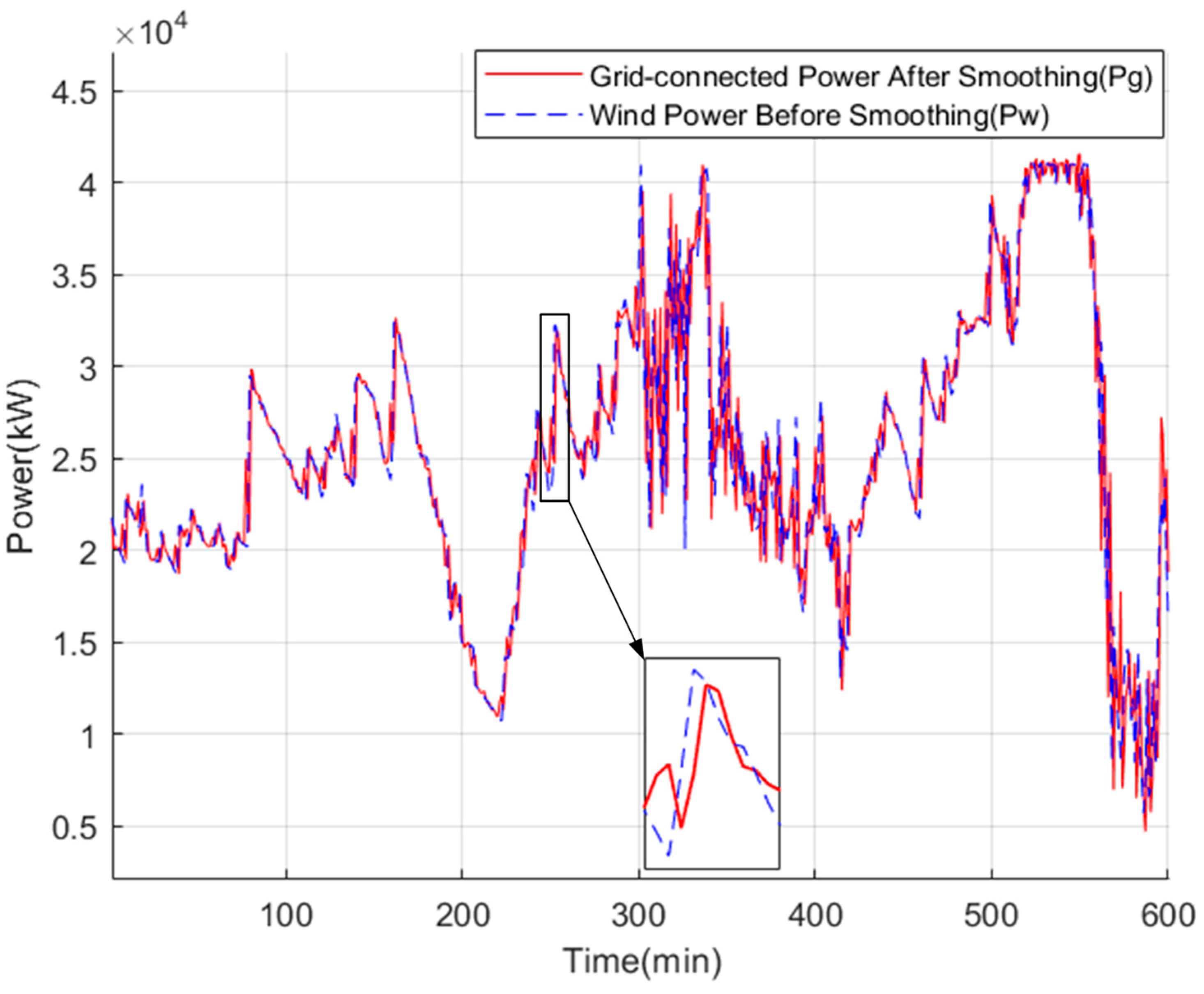
The wind power fluctuation needs to meet certain requirements for grid connection. The wind power grid connection conditions for the 50 MW wind farm studied in this paper are that the power fluctuation within 1 min should not exceed 1/10th of the installed capacity, and the power fluctuation within 10 min should not exceed 1/3rd of the installed capacity. On the other hand, the overall SOC constraints of the energy storage system must be considered. The goal of the control system is to reduce changes in power from the grid while keeping the SOC from becoming too high or too low. It also aims to avoid how often the battery needs to charge and discharge. The optimization model for the MPC algorithm is as follows:

(1)

State Space Equation

$$\left\{\begin{array}{l}{P}_g(k+1)=P_b(k)+P_w(k)\\ \mathrm{SOC}(k+1)=\mathrm{SOC}(k{)-\mathrm{T}}_{\mathrm{s}}{\mathrm{P}}_{\mathrm{b}}(k{)/\mathrm{E}}_{\mathrm{b}}\end{array}\right..$$

(6)

In Equation (6), k represents the control time node, P_g is the wind power grid connection power in kilowatts, and P_b is the total energy storage power in kilowatts, where positive and negative P_b values indicate energy storage discharge power and energy storage absorption power, respectively. Furthermore, SOC represents the overall state of charge of the energy storage system, E_b is the rated capacity of the energy storage in kilowatt-hours, and T_s is the control period in minutes.

(2)

Rolling Optimization Objective

Given the interdependence between wind power and energy storage, when the energy storage system has an adequate smoothing capacity, it should be utilized to minimize wind power fluctuations to the fullest extent. However, when the suppression capacity of energy storage is limited, the grid-connected fluctuations can be appropriately increased, or the energy storage output can be reduced, to restore the suppression capacity. Thus, considering the mutual constraints between the wind power fluctuation smoothing effect and the overall SOC of the energy storage, the overall target power of the hybrid energy storage system is optimized through a rolling process.

Building on the two points mentioned above, the optimization objective at time step k for the N prediction steps is as follows:

$$J=\min ({\displaystyle \sum _{i=1}^N(1-\omega (k)){(SOC(k+i)-0.5)}^2}+{\displaystyle \sum _{i=1}^N\omega }(k)({\displaystyle \frac{\Delta P_g(k+i-1)}{P_{w\_rate}}})).$$

(7)

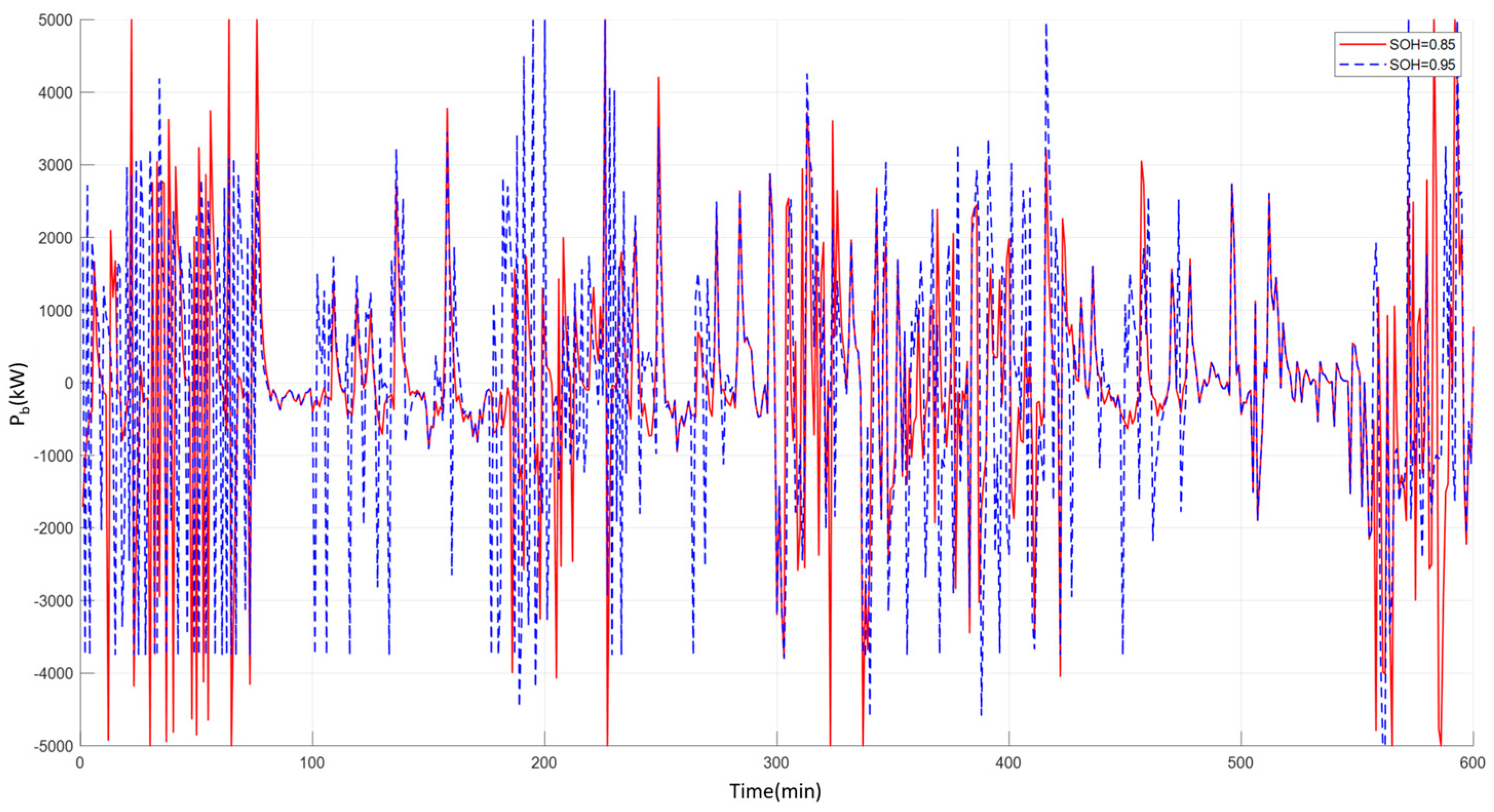
In Equation (7), ω(k) represents the charge and discharge capability index at time k, calculated based on the SOC and SOH of the hybrid energy storage system. A smaller value of ω(k) indicates reduced fluctuation in the grid-connected wind power relative to the wind farm’s generation power, and corresponds to a higher energy storage output. As the SOH of the energy storage declines, the dischargeable energy decreases as the SOC approaches its minimum value, resulting in a reduced discharge capability. The discharge depth required to release the same amount of energy will increase. The discharge depth is an important factor affecting energy storage health. Therefore, under different health conditions, the parameter ω can be adjusted to appropriately increase the wind power fluctuation under the condition of satisfying the grid-connected power fluctuation. This adjustment reduces the energy storage output, and prevents the situation where the energy storage’s health deteriorates more rapidly with the progression of usage time.

(3)

Constraints

The MPC must also satisfy the following constraints, including energy storage power constraints, SOC constraints, and wind power fluctuation constraints:

$$\left\{\begin{array}{l}-P_{\max }\le P\le P_{\max }\\ SO{C}_{\min }\le SOC\le SO{C}_{\max }\\ -T_s\delta \le \Delta P_g\le T_s\delta \end{array}\right.$$

(8)

In Equation (8), $SO{C}_{\min }$ and $SO{C}_{\max }$ are the minimum and maximum limits of the energy storage SOC, which are 0.1 and 0.9, respectively, $\delta$ is the fluctuation limit per unit time, set to 10% in this study, and Pmax is the maximum power constraint for the energy storage, which is equal to 8000 kW.

(4)

Solution Process

The MPC mathematical model can be obtained as follows by rewriting the state-space Equation (6) in the following form:

$$x(k+1)=Ax(k)+B_{u}u(k)+B_{r}r(k)$$

(9)

where the system’s state variables x(k) include the grid-connected power and the SOC of the energy storage, and are represented as:

$$x(k)=\left[\begin{array}{l}{P}_g(k)\\ SOC(k)\end{array}\right]$$

(10)

The system’s control variable u(k) is the total power of the storage, given as:

$$u(k)=\left[P_b(k)\right]$$

(11)

The system’s measurable disturbance input r(k) is the wind power, defined as follows:

$$r(k)=\left[P_w(k)\right]$$

(12)

Therefore, based on the relationships between the variables in Equation (6), the coefficient matrices in Equation (9) can be written as

$$\begin{array}{l}A=\left[\begin{array}{cc}0& 0\\ 0& 1\end{array}\right]\\ B_u=\left[\begin{array}{c}1\\ -T_s/E_b\end{array}\right]\\ B_r=\left[\begin{array}{c}1\\ 0\end{array}\right]\end{array}$$

(13)

At time k, x(k) is the known actual state value, and Equation (9) can be derived for time k + 1 as

$$x(k+2)=A^{2}x(k)+A{B}_{u}u(k)+A{B}_{r}r(k)+B_{u}u(k+1)+B_{r}r(k+1)$$

(14)

Let the state variable sequence, control variable, and disturbance sequence be

$$\begin{array}{l}{X}_k=\left[\begin{array}{l}x(k+1)\\ x(k+2)\\ \cdots \\ x(k+N)\end{array}\right]\\ U_k=\left[\begin{array}{l}u(k)\\ u(k+1)\\ \cdots \\ u(k+N-1)\end{array}\right]\\ R_k=\left[\begin{array}{l}r(k)\\ r(k+1)\\ \cdots \\ r(k+N-1)\end{array}\right]\end{array}$$

(15)

By analogy, the expression for the state variable at each time step can be obtained. Let x(k) = x₀, then Equation (9) can be extended as follows:

$$X_k=G{x}_0+I_u{U}_k+I_r{R}_k$$

(16)

The extended coefficient matrix is

$$\begin{array}{l}G=\left[\begin{array}{l}A\\ A^2\\ \dots \\ A^N\end{array}\right]\\ I_u=\left[\begin{array}{cccc}{B}_u& 0& \cdots & 0\\ A{B}_u& B_u& \cdots & 0\\ \cdots & \cdots & \cdots & \cdots \\ A^{N-1}{B}_u& A^{N-2}{B}_u& \cdots & B_u\end{array}\right]\\ I_r=\left[\begin{array}{cccc}{B}_r& 0& \cdots & 0\\ A{B}_r& B_r& \cdots & 0\\ \cdots & \cdots & \cdots & \cdots \\ A^{N-1}{B}_r& A^{N-2}{B}_r& \cdots & B_r\end{array}\right]\end{array}$$

(17)

Using this matrix operation, all state variables in the optimization objective can be represented by the control variables. The constant terms that do not participate in the optimization, are omitted. Subsequently, the objective function can be converted into a standard quadratic programming form as follows:

$$\min J={\displaystyle \frac{1}{2}}{U}_k^{T}H{U}_k+U_k^{T}f$$

(18)

In Equation (18), H and f denote the quadratic and linear coefficient matrices, respectively, corresponding to the control variables to be determined.

3.2. Fuzzy Control-Based Adaptive Adjustment of MPC Parameters

In the previous section, the power smoothing strategy based on the MPC algorithm considered the impact of the energy storage system’s SOC and wind power fluctuations on the minimum output of the energy storage system. However, the output capability of the energy storage system will gradually weaken as its health declines. In this case, it is necessary to appropriately reduce the energy storage output within the acceptable range of grid-connected power fluctuations. On the other hand, the energy storage output needs to be increased when wind power experiences severe fluctuations.

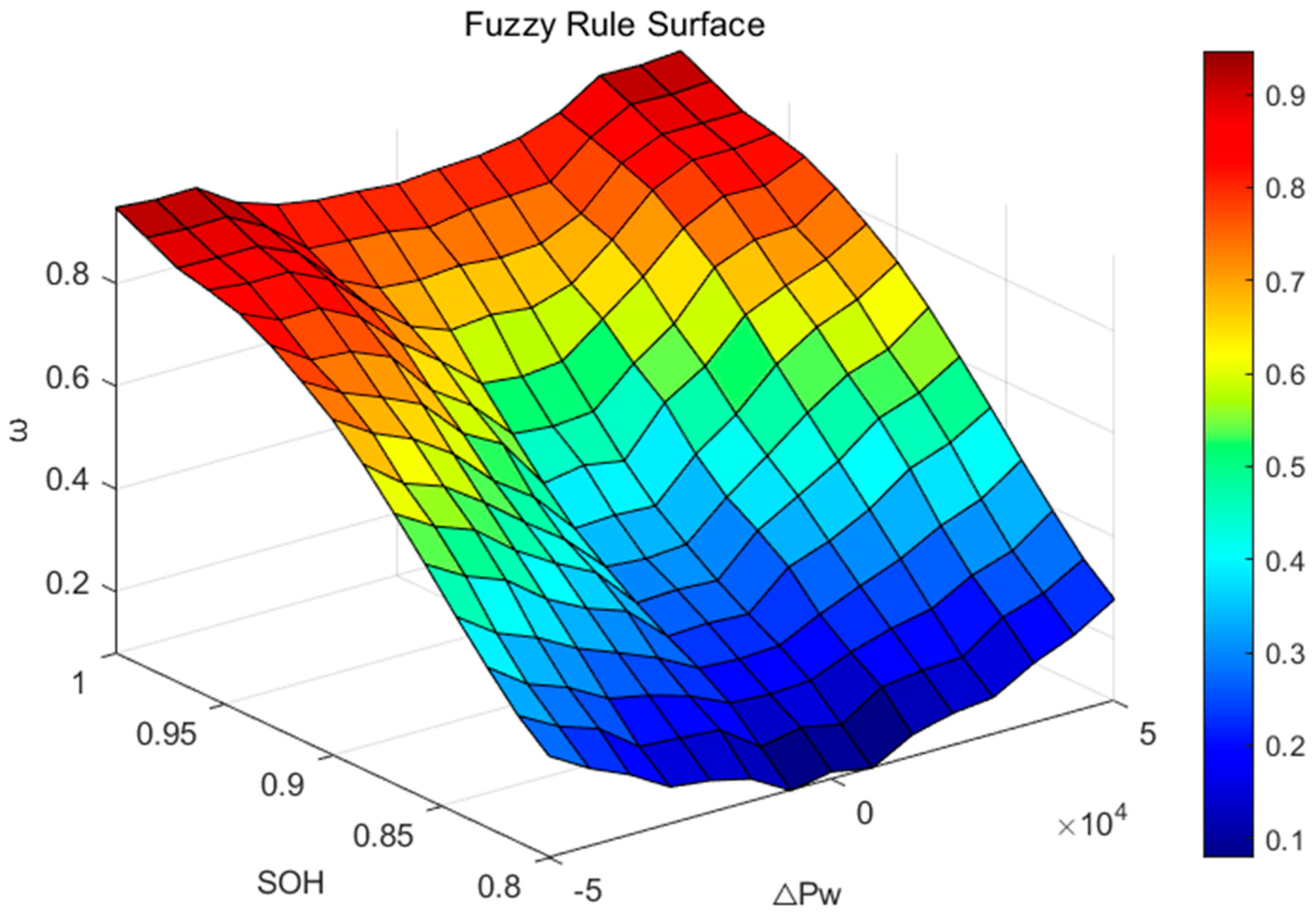
To optimize the control performance of the energy storage system, this study develops fuzzy control rules, using the SOH of the energy storage system and the active power variation relative to the previous minute as the input variables for the controller. The weight coefficient ω of the MPC is used as the control output to adaptively adjust the weight relationship between the energy storage battery’s output and the grid-connected power fluctuation suppression.

Specifically, under the same state of health of the energy storage battery, larger wind power fluctuations lead to greater energy storage output, while smaller wind fluctuations result in reduced output from the energy storage system. On the other hand, for the same wind power fluctuation, as the state of health of the energy storage battery decreases, its charging and discharging capacity is also reduced, which leads to a corresponding decrease in the energy storage output. Under the premise of meeting the grid connection requirements, this mechanism reduces the energy demand during the charging and discharging process, thus minimizing the negative impact on the battery’s health and balancing the trade-off between fluctuation suppression and battery lifespan.

This paper constructs the membership functions for the inputs and outputs using triangular shape functions, and designs the fuzzy linguistic values for each group as follows:

Input 1: This is the SOH value, with a continuous domain of [0.8, 1] and a fuzzy domain of {0.8, 0.85, 0.9, 0.95, 1}, corresponding to the fuzzy subsets {VS, S, M, L, VL}. These subsets represent the SOH values as {Very Small, Small, Medium, Large, Very Large}.

Input 2: At each moment, the change in active power of the wind farm relative to the previous minute has a continuous domain of [−20,000, 20,000], corresponding to a fuzzy domain of {−50,000, −30,000, −10,000, 10,000, 30,000, 50,000}, and the corresponding fuzzy subsets {NL, NM, NS, PS, PM, PL}. These subsets represent the current power fluctuation as {Negative Large, Negative Medium, Negative Small, Positive Small, Positive Medium, Positive Large}. When the discharge power signal is negative, it indicates a charging power signal.

Output: The continuous domain for the weight coefficient ω is [0, 1], with a fuzzy domain of {0, 0.0125, 0.0250, 0.0375, 0.0500, 0.0675, 0.0800, 0.0975, 1}, and the corresponding fuzzy subsets {ES, VS, S, MS, M, ML, L, VL, EL}. These subsets represent the weight coefficient values as {Extremely Small, Small, Medium Small, Medium, Medium Large, Large, Very Large, Extremely Large}.

Table 1. Fuzzy control rule table.

SOH	ΔPw
	NL	NM	NS	PS	PM	PL
VS	S	VS	ES	ES	VS	S
S	M	MS	S	S	MS	M
M	L	ML	MS	MS	ML	L
L	VL	VL	ML	ML	VL	VL
VL	EL	EL	VL	VL	EL	EL

shows the specific fuzzy control rules.

4. Simulation Analysis

This Section presents the experimental results, their interpretation, and the experimental conclusions.

4.1. Energy Storage Health Prediction

This Section uses a lithium-ion battery dataset provided by a company as the experimental object to train the energy storage health prediction algorithm and verify its accuracy. The dataset contains detailed charge and discharge cycle information, including the depth of discharge, the charge/discharge time, and the calendar aging time, i.e., the time since the battery was manufactured, which are used as input variables for the model. The capacity change recorded during each complete discharge process is used as the output variable. The GA-SVR algorithm’s accuracy in predicting the health status is validated based on this dataset.

The GA is used to optimize the SVR parameters, and the optimal SVR parameters are shown in Table 1. The model’s output obtained after the optimization of the three parameters is summarized in

Table 2. GA-SVR parameters.

GA-SVR Parameters
c	$\sigma$	$\epsilon$
4.85	3.03	0.0006

. In this study, the prediction results of the GA-SVR algorithm are compared with those of the Backpropagation (BP) algorithm, and the RMSE is used to evaluate prediction accuracy. The smaller the RMSE, the better the model’s prediction performance. Another metric is the coefficient of determination (R² value), which reflects the model’s ability to explain the data. A value closer to one indicates a better model.

Table 3. Comparison of prediction accuracy between GA-SVR and BP.

	Training Set		Test Set
	RMSE	R2	RMSE	R2
GA-SVR	5.0857 × 10−6	0.99451	5.2397 × 10−6	0.99475
BP	6.0691 × 10−6	0.99287	5.9216 × 10−6	0.99399

and Figure 4 show that the GA-SVR performs better than the BP in predicting the energy storage capacity loss and can more accurately predict the health status of the energy storage system.

Figure 4 illustrates the prediction performance of two algorithms, including their results on both the training and testing sets. Subplots (a) and (b) show the prediction performance of the BP algorithm, where subplot (a) represents the results on the training set, and subplot (b) shows the results on the testing set. Subplots (c) and (d) present the predictions of the algorithm proposed in this paper, where subplot (c) represents the results on the training set, and subplot (d) shows the results on the testing set. In each subplot, the blue dots represent the relationship between the predicted and actual values, with the horizontal axis indicating the predicted values and the vertical axis indicating the actual values. The yellow dashed line represents the ideal case where the predicted values exactly match the actual values. The closer the blue dots are to the yellow dashed line, the better the prediction performance is, with smaller deviations between the predicted and actual values, indicating higher prediction accuracy.

By comparing the predicted and measured data, the model fitting for two different datasets is analyzed. The health prediction results for the two forecasting algorithms are presented in Table 3. According to the parameter evaluation criteria outlined in Section 2.2.3, and based on the RMSE and R² values derived from the prediction results, it is clear that the GA-SVR algorithm exhibits superior accuracy. The

Table 4. Comparison of GA-SVR and BP energy SOH prediction results.

	1	2	3	4	5	6	7	…
Measured	1	0.98746	0.97941	0.96326	0.93455	0.92653	0.91848	…
GA-SVR	1	0.98745	0.97941	0.96327	0.93459	0.92655	0.91849	…
BP	1	0.98744	0.97940	0.96327	0.93458	0.92654	0.91848	…

below provides a comparison of the prediction performance between the GA-SVR and BP algorithms employed in this study. Since the table cannot accommodate all the experimental iterations, ’…’ is used to indicate the remaining data.

By inputting the battery’s charge and discharge data (including D, T_u, T_C, and DOD), the degradation of the usable capacity over the simulation time can be obtained. The current battery SOH is then calculated as the ratio of the predicted total capacity degradation to the initial capacity. The following shows the comparison between the measured SOH values and the predictions from the two algorithms:

The table presents the measured battery health values and the prediction results obtained by the two methods for experiments 1 to 7. The first row of the table lists the experiment numbers, the second row shows the measured battery health values for each experiment, and the third and fourth rows display the values predicted by the two methods. The table shows that both prediction methods perform well; however, the method proposed in this paper outperforms the other method in terms of prediction accuracy.

4.2. Grid-Connected Fluctuation Mitigation Effect and Energy Storage Power Optimization Results

A model is built and simulated in MATLAB R2022b to verify the effectiveness of the strategy proposed in this paper. The input data used in the simulations consist of wind power data from a wind farm with an installed capacity of 50 MW. The wind power data are sampled at a sampling interval of one minute, over 10 h. The MPC prediction horizon is set to five minutes, with a control period of one minute. The total energy storage capacity is assumed to be 1000 kWh, with an initial SOC of 0.5 and SOC limits of 0.9 and 0.1, respectively.

4.2.1. Grid-Connected Power Fluctuation Mitigation Effect

The initial health index of the energy storage system and the unit-time fluctuation limit are set to 0.95 and 10%, respectively. The corresponding results after fluctuation mitigation of the original wind power output are shown in Figure 5. It can be observed that the wind power curve becomes significantly smoother after fluctuation mitigation.

Table 5. Comparison of fluctuation rates between raw wind power and grid-connected power.

	Raw Wind Power	Grid-Connected Wind Power
1 min	11.03%	8.05%
10 min	34.59%	26.42%

shows the average fluctuation rates of wind power before and after smoothing over 1 min and 10 min time scales, respectively. The fluctuation rate is calculated as the maximum fluctuation amplitude divided by the rated capacity of the wind power. It can be observed from the table that the average fluctuation rate decreases significantly for both time scales. The decrease is approximately 2.98% and 8.17% for the 1 min and 10 min scales, respectively. These results demonstrate that the control strategy effectively reduces large fluctuations and improves the wind power output stability.

Next, the smoothed wind power curve is analyzed to evaluate whether it meets the grid connection requirements. Table 5 further presents the maximum fluctuation rates of wind power before and after smoothing on 1 min and 10 min time scales. For an installed capacity of 50 MW, the maximum allowable fluctuation rate is 10% for 1 min and 33% for 10 min. It can be observed that the wind power curve after fluctuation smoothing meets the Chinese national grid connection standards.

The power fluctuations are extracted and the distributions before and after smoothing are compared in Figure 6. It can be observed that the raw wind power has a maximum fluctuation of 16 MW, while the maximum fluctuation after smoothing is 14 MW. The fluctuation of the grid-connected power after smoothing is more concentrated, with a higher proportion of low fluctuations. These results indicate that the control strategy effectively reduces high fluctuations and reduces the wind power volatility.

4.2.2. Energy Storage Power Optimization

The weight coefficient ω of the MPC objective function represents the trade-off between the energy storage system output and the severity of grid-connected power fluctuations. A larger coefficient indicates a higher requirement for energy storage output, which results in a better smoothing effect. Before introducing fuzzy control, ω is set to a fixed value of 0.5. After introducing fuzzy control, the system can dynamically adjust ω based on the energy storage’s SOH and the fluctuations’ severity. When the energy storage SOH is low, fuzzy control reduces the weight of energy storage output, which extends the system’s lifespan. For severe fluctuations, fuzzy control increases the energy storage system output to better smoothen the fluctuations. This adaptive mechanism improves the overall performance of the energy storage system, preventing excessive discharge when the SOH is low, while providing a more effective stable output during severe fluctuations.

Figure 7 visually demonstrates the fuzzy control rules by plotting the three-dimensional response surface of the fuzzy controller. The energy storage’s SOH is given on the X-axis, while the Y-axis represents the power fluctuations within a range of −50,000 to 50,000. Both the SOH and power fluctuation are used as input variables, and ω is the output variable. After introducing fuzzy control, ω decreases as the energy storage’s SOH declines, and it increases as fluctuations become more severe, reflecting the system’s adaptive adjustment characteristics.

Figure 8 shows the energy storage power under fuzzy control adjustment while ensuring that the grid-connected power meets the grid fluctuation requirements. Initial energy storage SOH values of 0.95 and 0.85 are considered.

The comparison of energy storage charging and discharging energy and grid-connected power fluctuation rates under different SOH conditions is shown in

Table 6. Comparison of energy storage output and grid-connected power fluctuation rates under different SOH conditions.

SOH	Total Charging and Discharging Energy/kWh	10 min Grid-Connected Power Fluctuation Rate
0.95	1.4228 × 105	26.42%
0.85	1.0946 × 105	32.86%

.

Table 6 compares the energy storage charging and discharging energy and grid-connected power fluctuation rates under different SOH conditions. It can be observed that under the same wind power scenario, when the SOH = 0.95, the total charging and discharging energy of the energy storage system is 1.4228 × 105 kWh. On the other hand, when the SOH = 0.85, the total charging and discharging energy is 1.0946 × 105 kWh. The corresponding 10 min grid-connected power fluctuation rate is calculated by dividing the maximum fluctuation amplitude by the rated wind power capacity. This rate is equal to 26.42% and 32.86% for a SOH = 0.95 and 0.85, respectively.

When the health status of the energy storage battery is 0.9, the total simulation time is set to 600 min. During this period, since the health status of the energy storage battery changes minimally, the variation can be ignored, and it is assumed that the health status remains constant at 0.9. In the first 300 min of the simulation, the average fluctuation rate of the wind power output is 16.18%; in the subsequent 300 min, the average fluctuation rate of the wind power output decreases to 7.94%, indicating a reduction in volatility. Meanwhile, thanks to the fuzzy control rules, the output of the energy storage system was adaptively adjusted and correspondingly reduced. The total charge and discharge energy of the energy storage system decreased from 4.898 × 10³ kWh in the first 300 min to 2.424 × 10³ kWh in the latter 300 min; the fluctuation rate of the grid-connected power was also significantly reduced, from 12.63% in the first 300 min to 3.48% in the latter 300 min.

These results indicate that the fuzzy control rule demonstrates high adaptability under the premise of ensuring grid-connected power fluctuation limits. When the energy storage system has a high SOH, under the same fluctuation conditions, the fuzzy control tends to increase the energy storage output that results in the enhanced smoothing of grid fluctuations. When the SOH is lower, the control rule tends to reduce the energy storage output, which prioritizes the protection of the energy storage system and sacrifices part of the smoothing effect to reduce the wear and tear of the storage equipment and extend its lifespan.

5. Conclusions

This paper proposed a prediction algorithm aimed at forecasting the SOH of energy storage to control the energy storage output and suppress fluctuations in wind power grid connection. First, the GA-SVR algorithm was used to train a prediction model with existing charging and discharging power data and available capacity data, and the network’s prediction performance was tested. Second, fuzzy control was applied to improve the MPC algorithm and adaptively adjust the weight between energy storage output and fluctuation levels. This method enhanced the reliability of energy storage for assisting wind power grid connection under different health states. Last, considering the grid fluctuation rate constraint and energy storage SOC, the MPC smoothing strategy was employed to alleviate wind power fluctuations and obtain energy storage output and grid-connected power. Our future work will consist of further improving the smoothing strategies and the corresponding prediction methods.