
Euclidean Distance-Based Tree Algorithm for Fault Detection and Diagnosis in Photovoltaic Systems

 , and
, and
Abstract
1. Introduction
2. Proposed Euclidean-Based Decision Tree Classification Algorithm
- (a)
- Choose an arbitrary point in an -dimensional space.
- (b)
- Using Equations (1) and (2), compute the Euclidean distances between the chosen point and all samples within the training dataset for each respective class:
- (c)
- Determine the minimum and maximum distances for each class:
- (d)
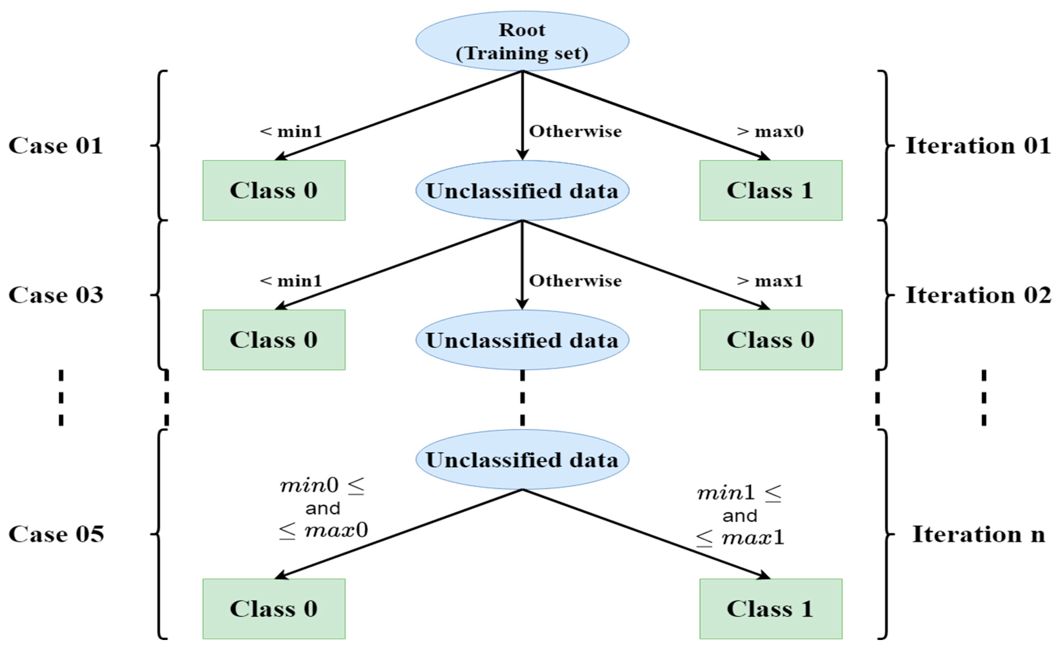
- Merge the two vectors and into one vector. Then, arrange the vector in ascending order. Among the following five cases, one may arise:
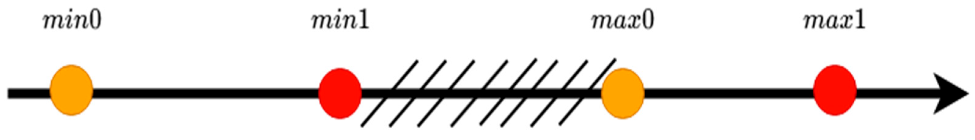
- case 1:Figure 1 shows a graphical representation of the first case.
- -
- Training sample shaving distances within the interval belong to class 0 (pure data in class 0).
- -
- Training samples having distances within the interval belong to class 1 (pure data in class 1).
- -
- Training samples having distances within the interval cannot be classified; therefore, another random point must be chosen for their classification.
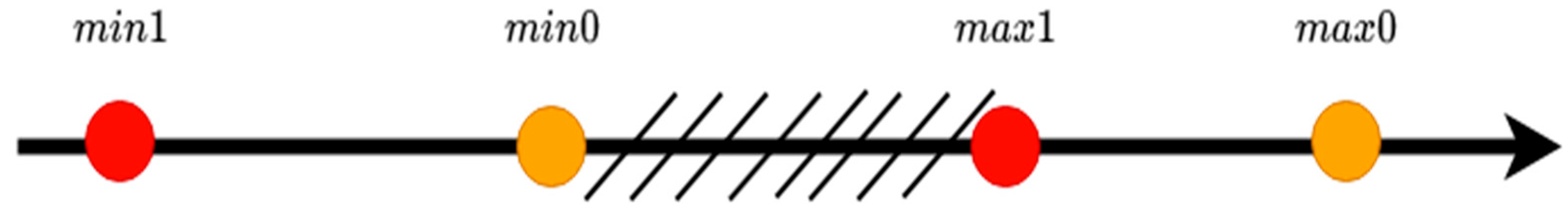
- case 2:Figure 2 shows a graphical representation of the second case.
- -
- Training samples having distances within the interval belong to class 1 (pure data in class 1).
- -
- Training samples having distances within the interval belong to class 0 (pure data in class 0).
- -
- Training samples having distances within the interval cannot be classified; therefore, another random point must be chosen for their classification.
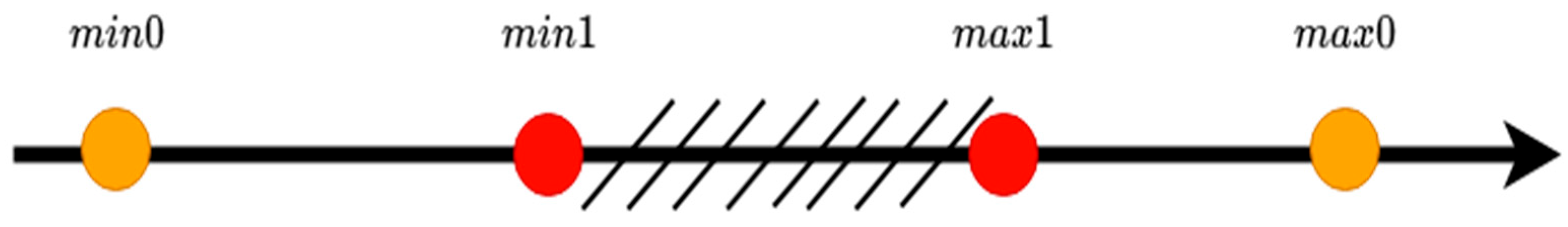
- case 3:Figure 3 shows a graphical representation of the third case.
- -
- Training samples having distances within the interval or belong to class 0.
- -
- Training samples having distances within the interval cannot be classified; therefore, another random point must be chosen for their classification.
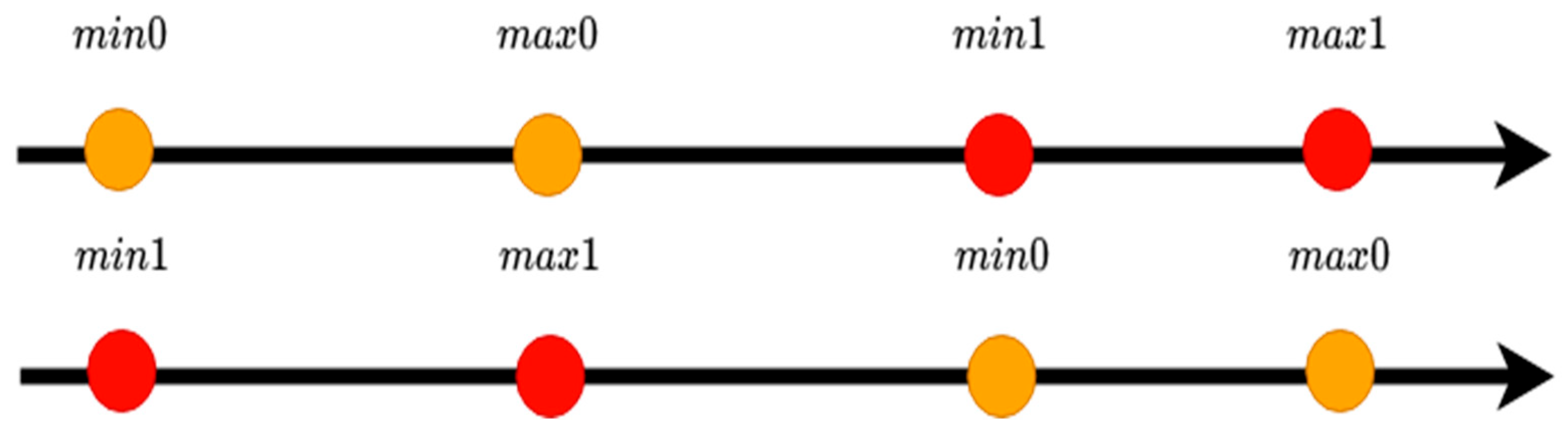
- case 4:Figure 4 shows a graphical representation of the forth case.
- -
- Training samples having distances within the interval or belong to class 0.
- -
- Training samples having distances within the interval cannot be classified; therefore, another random point must be chosen for their classification.
- case 5: orFigure 5 shows a graphical representation of the fifth case.
- -
- Training samples having distances within the interval belong to class 0.
- -
- Training samples having distances within the interval belong to class 1.
- (e)
- If the case that occurred in the previous step is case 1, 2, 3, or 4:
- -
- Choose another random point .
- -
- Using Equations (1) and (2), compute the Euclidean distances between the chosen points and the unclassified samples within the training dataset for each respective class.
- -
- Go to step (c).
- (f)
| Algorithm 1. Pseudo-code of the proposed algorithm |
| STEP (a): Generate a random point. STEP (b): Using Equations (1) and (2), calculate the distances and . STEP (c): Find , the minimal and maximal distances of each class. STEP (d): Store the computed di-stances int a vector named and organize it in ascending order. STEP (e): (the counter for unclassified data) - If For to () If The point associated to belongs to elseif The point associated to belongs to Else () Increment End if END for . if the stopping criteria is not verified Choose a new arbitrary point. Calculate the distances and for unclassified data. Go to step (c). Else Go to step (f). End if Elseif For to If The point associated to belongs to elseif The point associated to belongs to Else () Increment End if END for . if the stopping criteria is not verified Choose a new arbitrary point. Calculate the distances and for unclassified data. Go to step (c). Else Go to step (f). End if. Elseif For to If or The point associated to belongs to Else () Increment End if END for . if the stopping criteria is not verified Choose a new arbitrary point. Calculate the distances and for unclassified data. Go to step (c). Else Go to step (f). End if. Elseif For to If or The point associated to belongs to Else () Increment End if END for . if the stopping criteria is not verified Choose a new arbitrary point. Calculate the distances and for unclassified data. Go to step (c). Else Go to step (f). End if. Else (() or ()) For to If The point associated to belongs to If The point associated to belongs to END for Go to step (f) End if Step (f): End (all data are classified or the stopping criterion is met). |
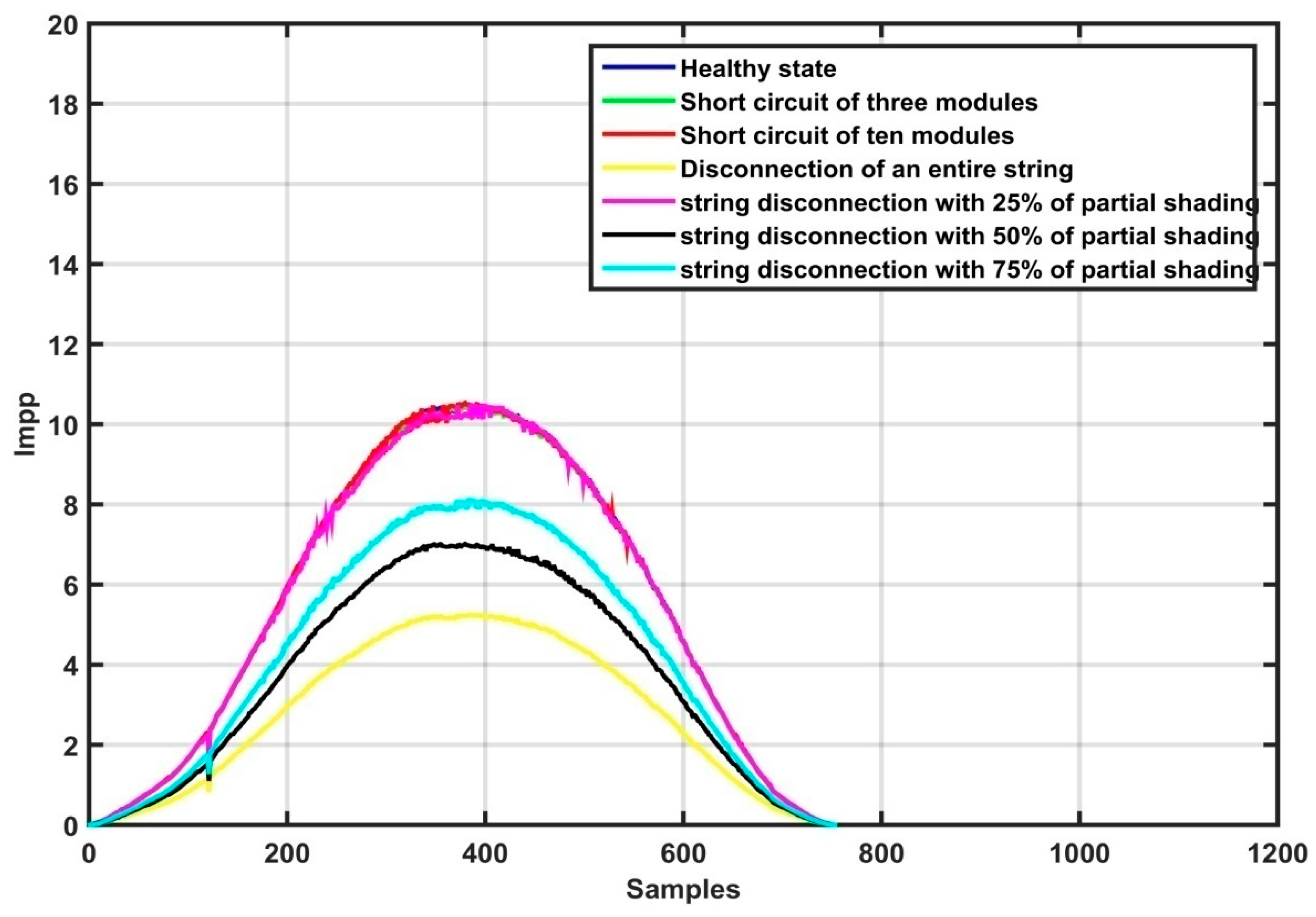
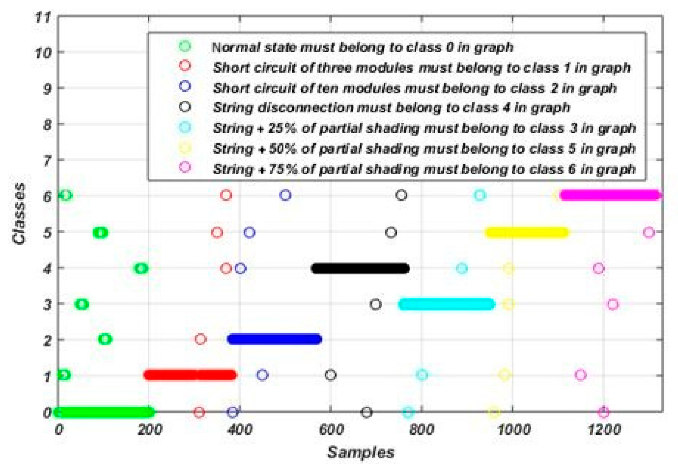
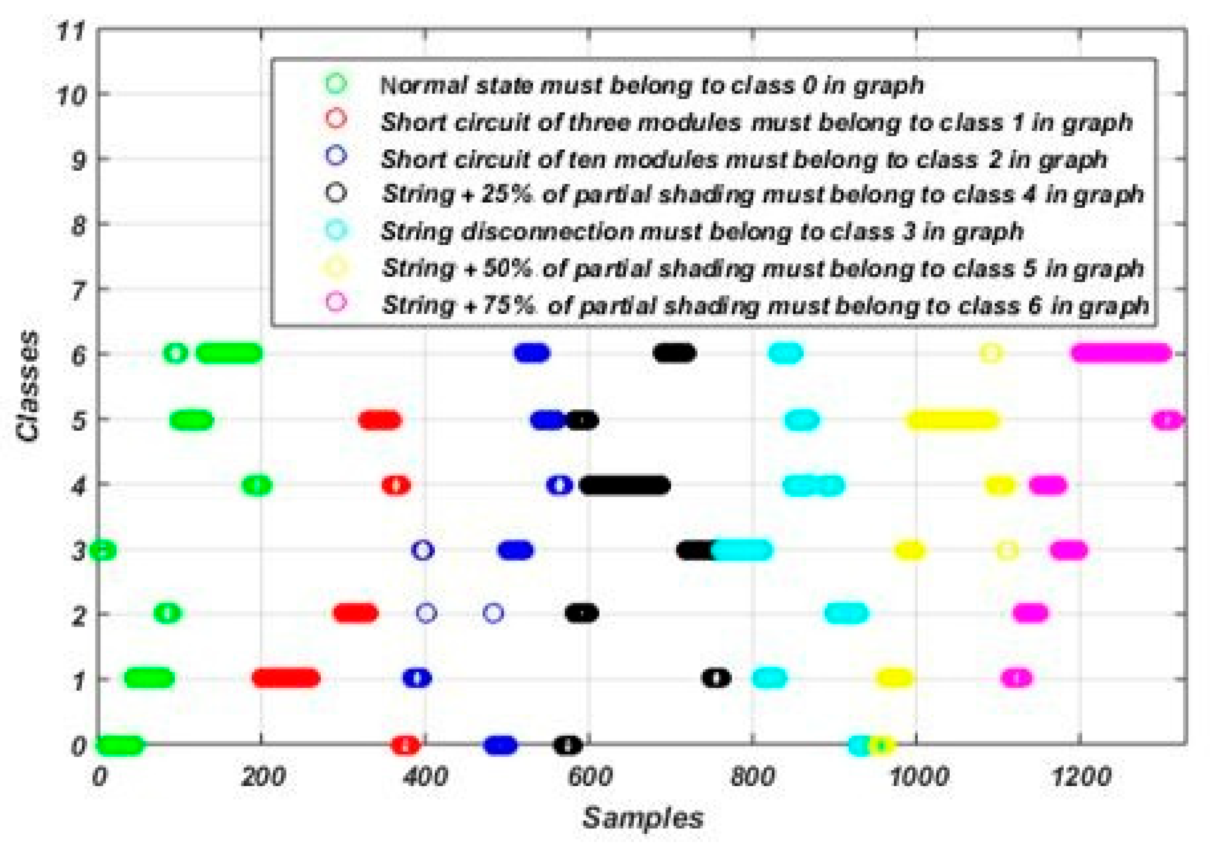
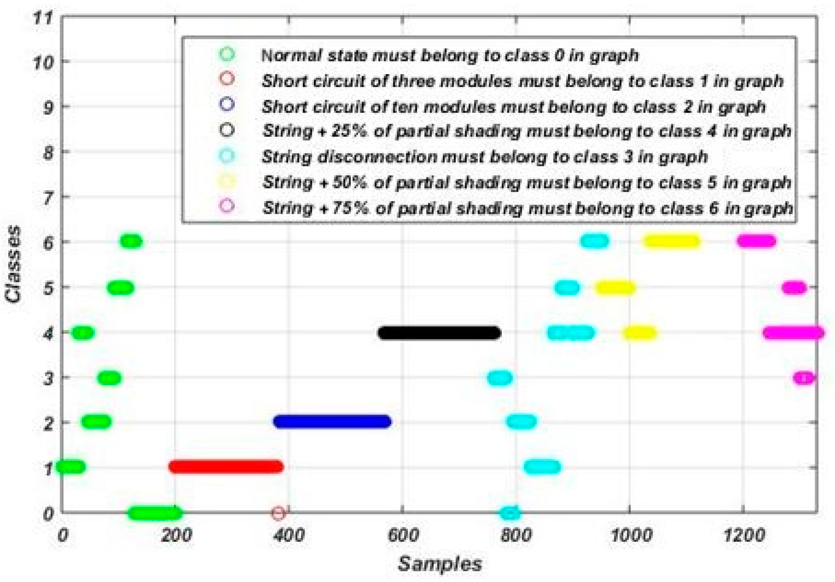
3. Dataset Description
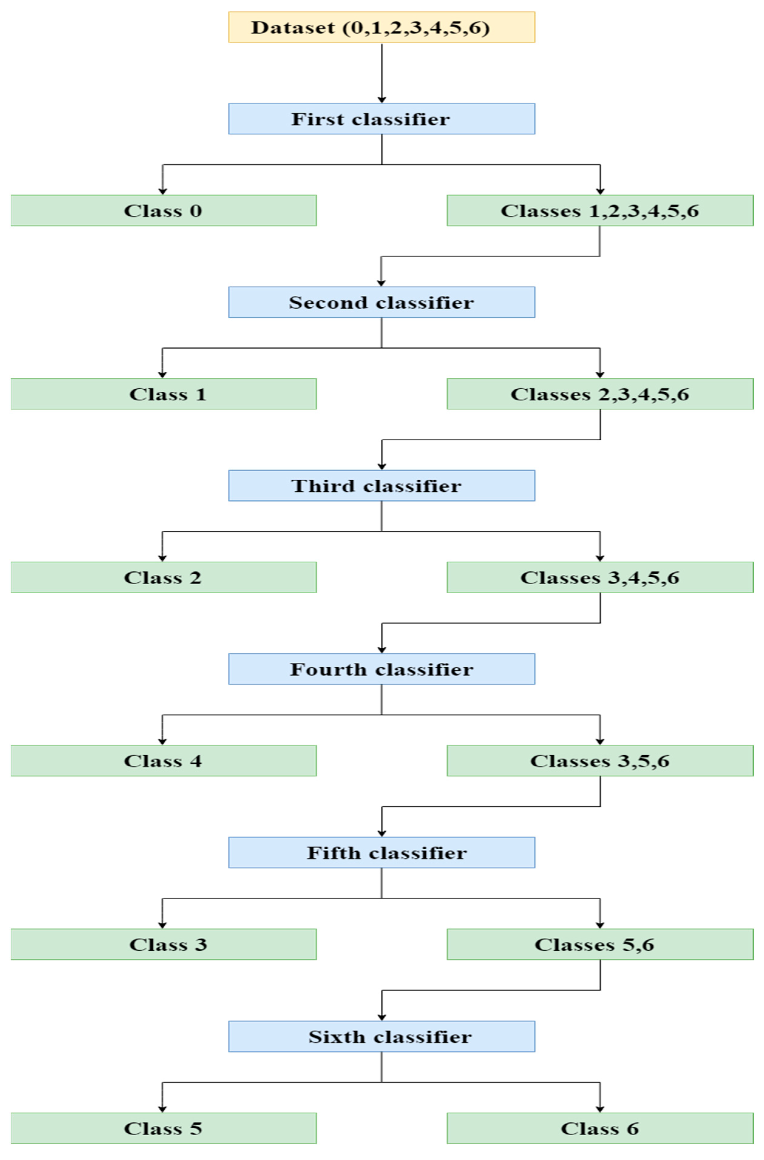
4. Fault Detection and Diagnosis Methodology
5. Results and Discussion
- Accuracy: A metric that shows how many data the algorithm correctly classifies. It is given by
- Precision: Measures the proportion of correctly predicted positive data to the total data predicted as positive. It is given by
- Recall: A metric that shows how many data that are really in class 1 which the classifier correctly predicted to be in class 1. It is given by
- F1-score: Measures the harmonic mean between the precision and the recall. It is given by
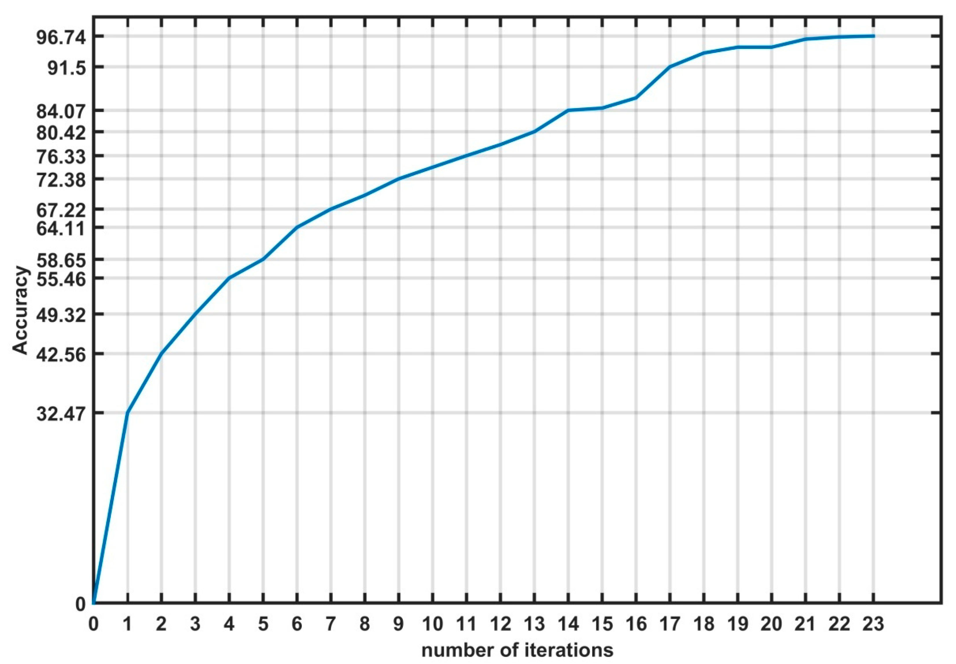
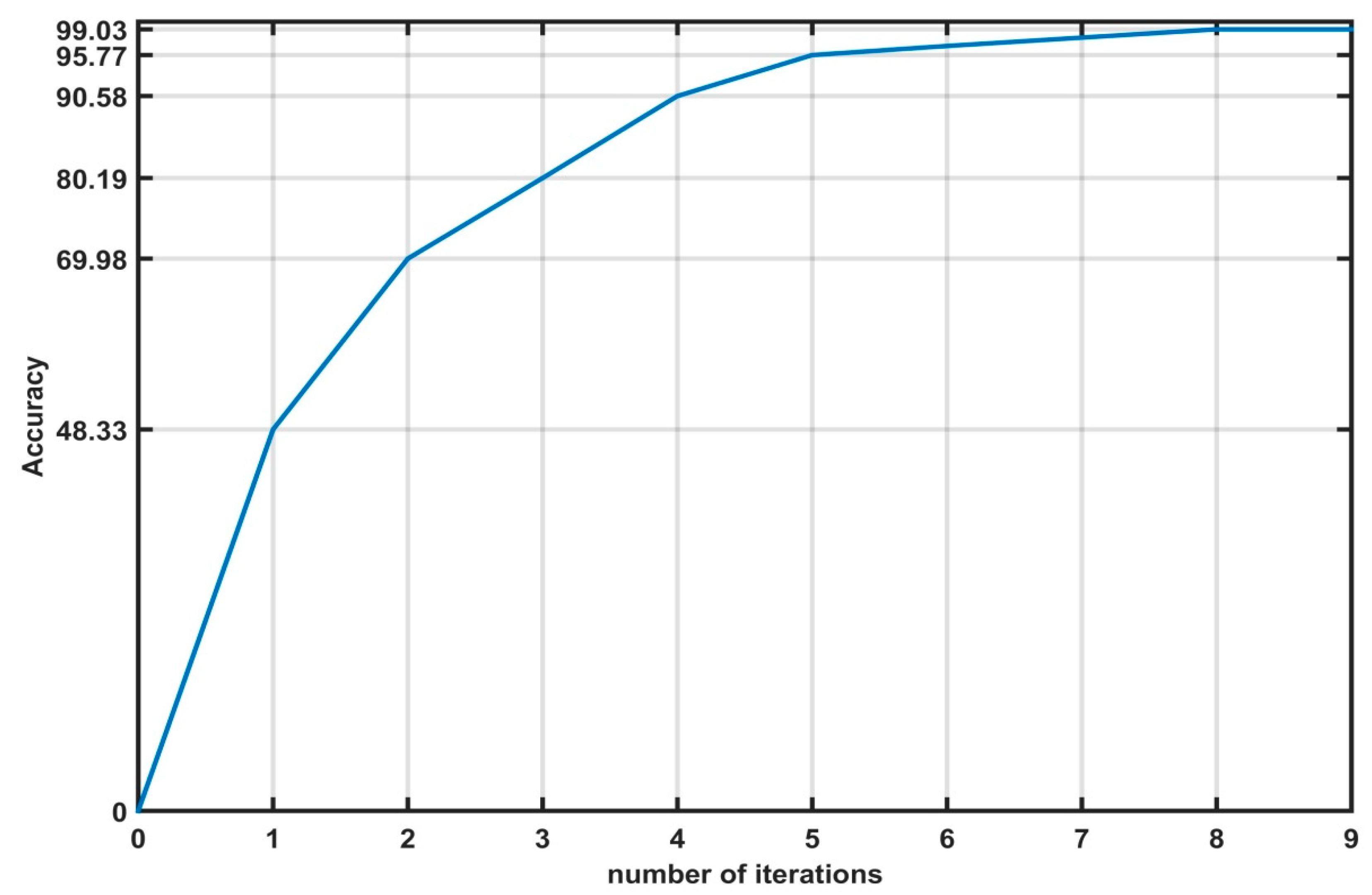
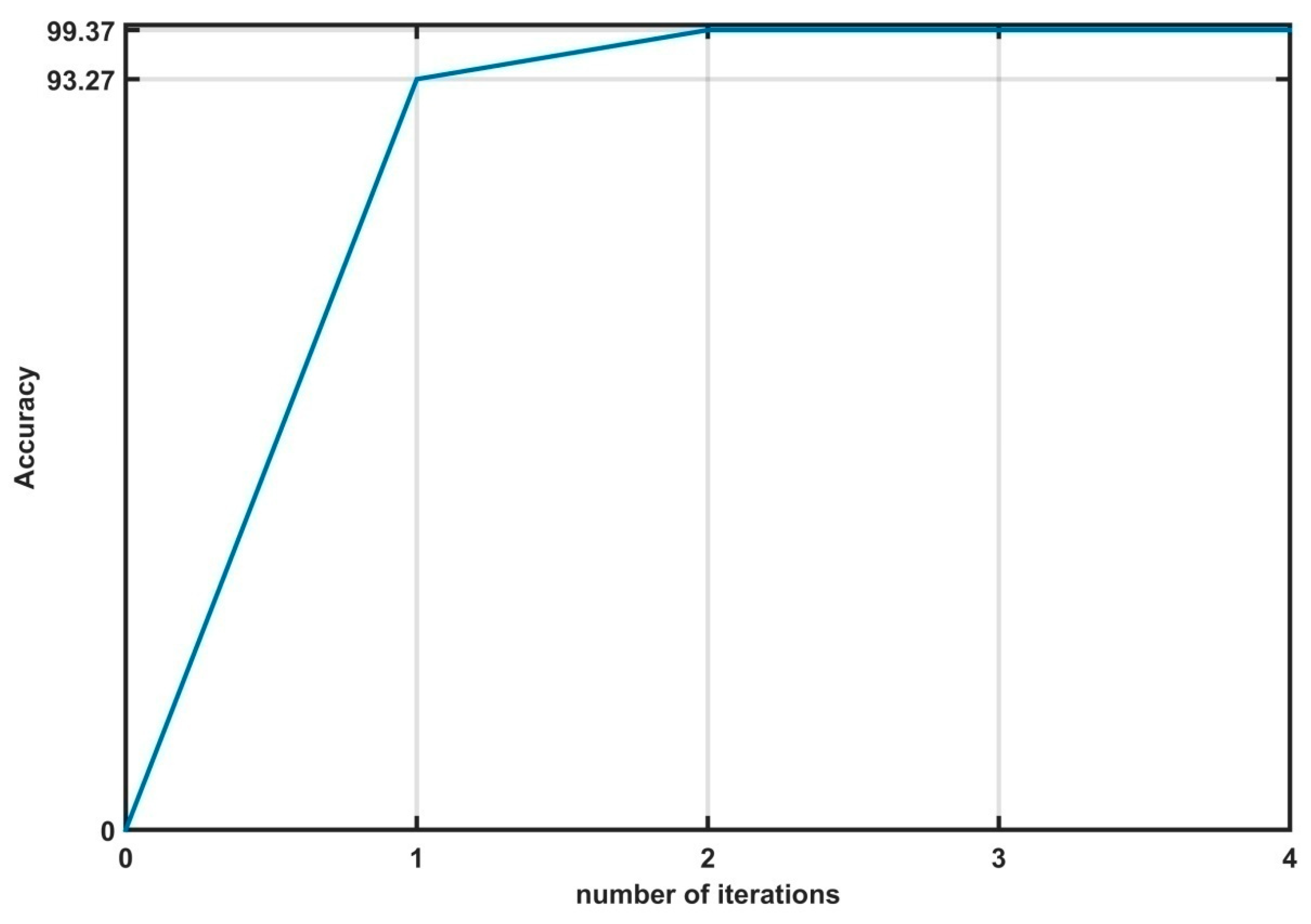
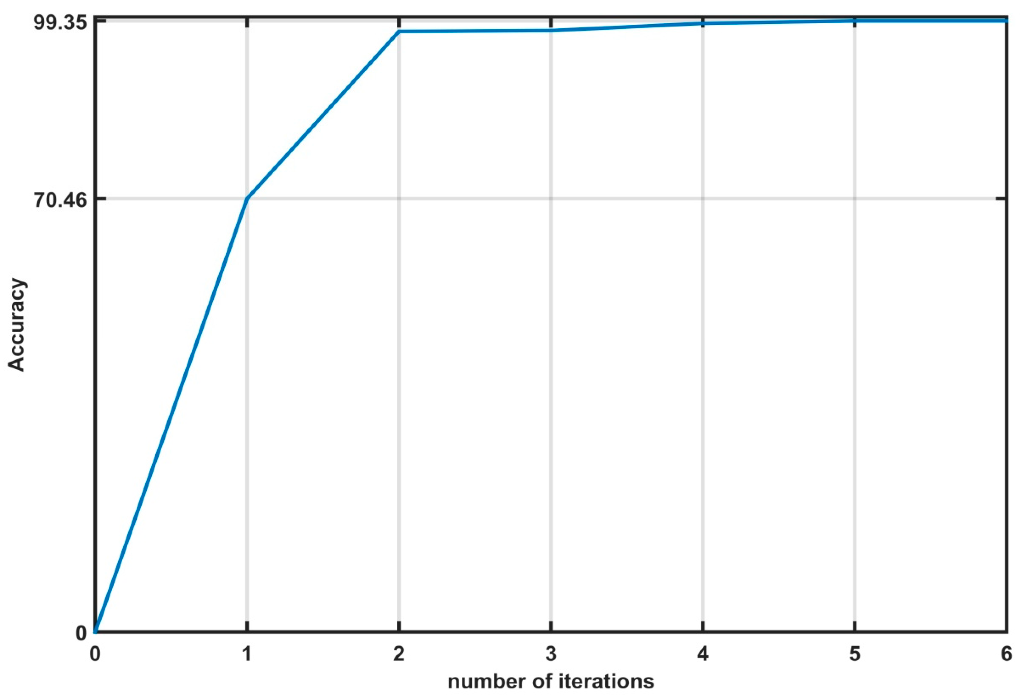
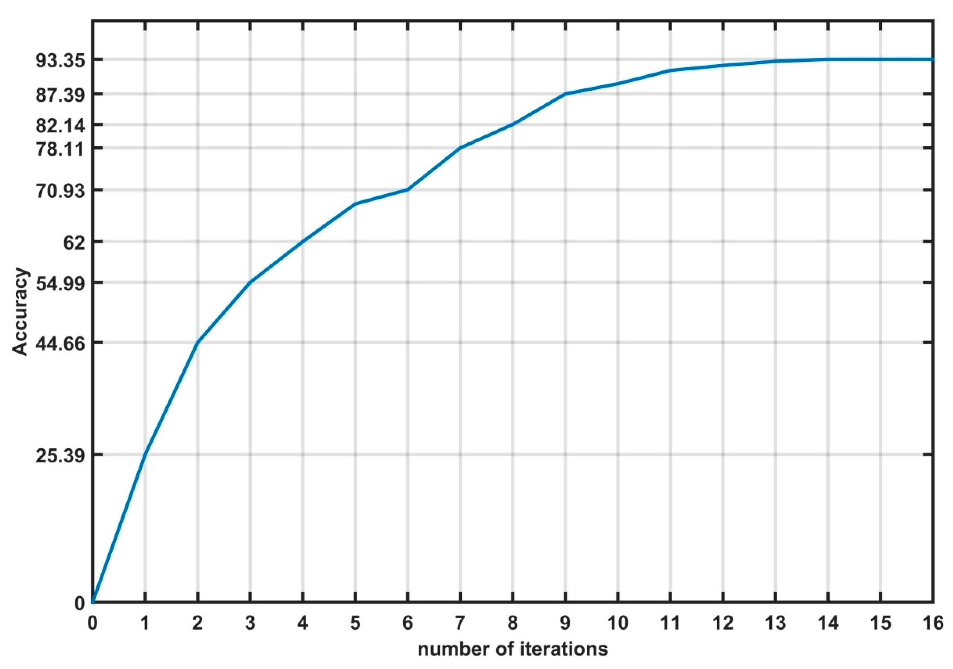
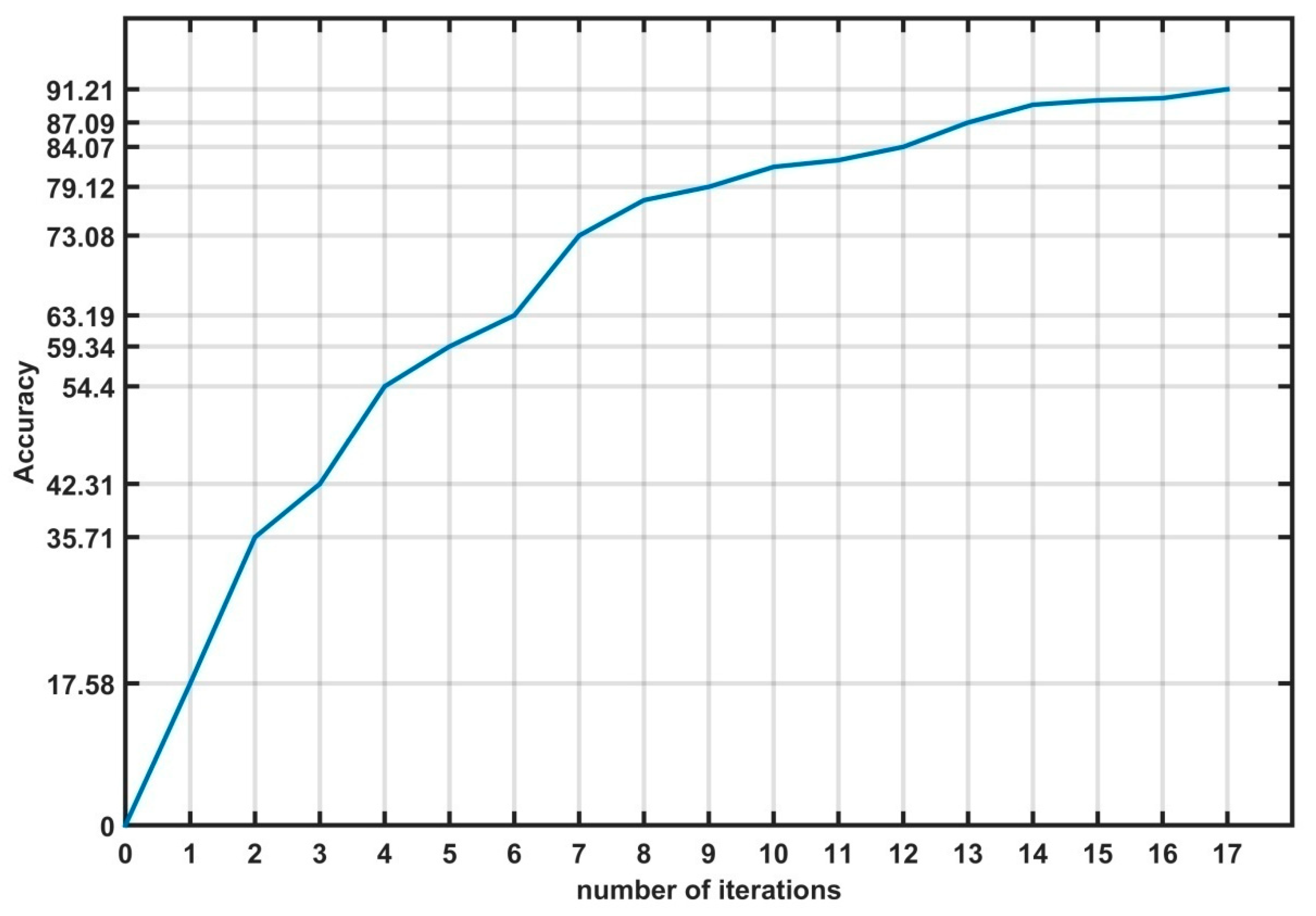
5.1. Training the Fault Detection and Diagnosis Model Using the Proposed Algorithm
5.2. Evaluating the Performance of the Obtained Model Using the Proposed Algorithm
5.3. Comparative Studyy of Various Machine Learning Algorithms
6. Conclusions
Author Contributions
Funding
Data Availability Statement
Conflicts of Interest
Abbreviations
| ADAG | Adaptive directed acyclic graph |
| ANN | Artificial neural network |
| DDAG | Decision directed acyclic graph |
| DT | Decision Tree |
| FDD | Fault Detection and Diagnosis |
| FN | False Negative |
| FP | False Positive |
| G | Irradiance |
| GCPV | Grid connected photovoltaic |
| Impp | Current at the maximum power point |
| Isc | Current of short circuit |
| KNN | K-Nearest Neighbors |
| OVA | One vs. all |
| PV | Photovoltaic |
| PVM | Photovoltaic module |
| PVS | Photovoltaic system |
| RF | Random Forest |
| SVM | Support Vector Machine |
| T | Temperature |
| TDR | Time domain reflectometry |
| TN | True Negative |
| TP | True Positive |
| Vmpp | Voltage at the maximum power point |
| Voc | Voltage of open circuit |
References
- Sohani, A.; Sayyaadi, H.; Cornaro, C.; Shahverdian, M.; Pierro, M.; Moser, D.; Karimi, N.; Doranehgard, M.; Li, L.K. Using machine learning in photovoltaics to create smarter and cleaner energy generation systems: A comprehensive review. J. Clean. Prod. 2022, 364, 132701. [Google Scholar]
- Mughal, S.; Sood, Y.R.; Jarial, R. A review on solar photovoltaic technology and future trends. Int. J. Sci. Res. Comput. Sci. Eng. Inf. Technol. 2018, 4, 227–235. [Google Scholar]
- Madeti, S.R.; Singh, S. A comprehensive study on different types of faults and detection techniques for solar photovoltaic system. Sol. Energy 2017, 158, 161–185. [Google Scholar]
- Hernandez, J.; Velasco, D.; Trujillo, C. Analysis of the effect of the implementation of photovoltaic systems like option of distributed generation in Colombia. Renew. Sustain. Energy Rev. 2011, 15, 2290–2298. [Google Scholar]
- Qais, M.H.; Hasanien, H.M.; Alghuwainem, S.; Nouh, A.S. Coyote optimization algorithm for parameters extraction of three-diode photovoltaic models of photovoltaic modules. Energy 2019, 187, 116001. [Google Scholar]
- Kumar, B.P.; Ilango, G.S.; Reddy, M.J.B.; Chilakapati, N. Online fault detection and diagnosis in photovoltaic systems using wavelet packets. IEEE J. Photovolt. 2017, 8, 257–265. [Google Scholar]
- Benkercha, R.; Moulahoum, S. Fault detection and diagnosis based on C4.5 decision tree algorithm for grid connected PV system. Sol. Energy 2018, 173, 610–634. [Google Scholar]
- Villarini, M.; Cesarotti, V.; Alfonsi, L.; Introna, V. Optimization of photovoltaic maintenance plan by means of a FMEA approach based on real data. Energy Convers. Manag. 2017, 152, 1–12. [Google Scholar]
- Pillai, D.S.; Rajasekar, N. A comprehensive review on protection challenges and fault diagnosis in PV systems. Renew. Sustain. Energy Rev. 2018, 91, 18–40. [Google Scholar]
- Zhao, Q.; Shao, S.; Lu, L.; Liu, X.; Zhu, H. A new PV array fault diagnosis method using fuzzy C-mean clustering and fuzzy membership algorithm. Energies 2018, 11, 238. [Google Scholar] [CrossRef]
- Hazra, A.; Das, S.; Basu, M. An efficient fault diagnosis method for PV systems following string current. J. Clean. Prod. 2017, 154, 220–232. [Google Scholar]
- Khelil, C.K.M.; Amrouche, B.; Soufiane Benyoucef, A.; Kara, K.; Chouder, A. New intelligent fault diagnosis (IFD) approach for grid-connected photovoltaic systems. Energy 2020, 211, 118591. [Google Scholar]
- Khelil, C.K.M.; Amrouche, B.; Kara, K.; Chouder, A. The impact of the ANN’s choice on PV systems diagnosis quality. Energy Convers. Manag. 2021, 240, 114278. [Google Scholar]
- Mellit, A.; Tina, G.M.; Kalogirou, S.A. Fault detection and diagnosis methods for photovoltaic systems: A review. Renew. Sustain. Energy Rev. 2018, 91, 1–17. [Google Scholar]
- Takashima, T.; Yamaguchi, J.; Otani, K.; Kato, K.; Ishida, M. Experimental studies of failure detection methods in PV module strings. In Proceedings of the 2006 IEEE 4th World Conference on Photovoltaic Energy Conference, Waikoloa, HI, USA, 7–12 May 2006; Volume 2, pp. 2227–2230. [Google Scholar]
- Takashima, T.; Yamaguchi, J.; Ishida, M. Fault detection by signal response in PV module strings. In Proceedings of the 2008 33rd IEEE Photovoltaic Specialists Conference, San Diego, CA, USA, 11–16 May 2008; pp. 1–5. [Google Scholar]
- Takashima, T.; Yamaguchi, J.; Otani, K.; Oozeki, T.; Kato, K.; Ishida, M. Experimental studies of fault location in PV module strings. Sol. Energy Mater. Sol. Cells 2009, 93, 1079–1082. [Google Scholar]
- Takashima, T.; Yamaguchi, J.; Ishida, M. Disconnection detection using earth capacitance measurement in photovoltaic module string. Prog. Photovolt. Res. Appl. 2008, 16, 669–677. [Google Scholar] [CrossRef]
- Chouder, A.; Silvestre, S. Automatic supervision and fault detection of PV systems based on power losses analysis. Energy Convers. Manag. 2010, 51, 1929–1937. [Google Scholar]
- Silvestre, S.; Chouder, A.; Karatepe, E. Automatic fault detection in grid connected PV systems. Sol. Energy 2013, 94, 119–127. [Google Scholar] [CrossRef]
- Spataru, S.; Sera, D.; Kerekes, T.; Teodorescu, R. Photovoltaic array condition monitoring based on online regression of performance model. In Proceedings of the 2013 IEEE 39th Photovoltaic Specialists Conference (PVSC), Tampa, FL, USA, 16–21 June 2013; pp. 0815–0820. [Google Scholar]
- Drews, A.; De Keizer, A.; Beyer, H.G.; Lorenz, E.; Betcke, J.; Van Sark, W.; Heydenreich, W.; Wiemken, E.; Stettler, S.; Toggweiler, P.; et al. Monitoring and remote failure detection of grid-connected PV systems based on satellite observations. Sol. Energy 2007, 81, 548–564. [Google Scholar]
- Bastidas-Rodriguez, J.D.; Franco, E.; Petrone, G.; Ramos-Paja, C.A.; Spagnuolo, G. Quantification of photovoltaic module degradation using model based indicators. Math. Comput. Simul. 2017, 131, 101–113. [Google Scholar]
- Dhoke, A.; Sharma, R.; Saha, T.K. An approach for fault detection and location in solar PV systems. Sol. Energy 2019, 194, 197–208. [Google Scholar]
- Mandal, R.K.; Kale, P.G. Assessment of different multiclass SVM strategies for fault classification in a PV system. In Proceedings of the Proceedings of the 7th International Conference on Advances in Energy Research, Singapore, 13–15 August 2019; Springer: Singapore, 2021; pp. 747–756. [Google Scholar]
- Cho, K.H.; Jo, H.C.; Kim, E.s.; Park, H.A.; Park, J.H. Failure diagnosis method of photovoltaic generator using support vector machine. J. Electr. Eng. Technol. 2020, 15, 1669–1680. [Google Scholar]
- Chen, L.; Lin, P.; Zhang, J.; Chen, Z.; Lin, Y.; Wu, L.; Cheng, S. Fault diagnosis and classification for photovoltaic arrays based on principal component analysis and support vector machine. IOP Conf. Ser. Earth Environ. Sci. 2018, 188, 012089. [Google Scholar]
- Wang, J.; Gao, D.; Zhu, S.; Wang, S.; Liu, H. Fault diagnosis method of photovoltaic array based on support vector machine. Energy Sources Part A Recovery Util. Environ. Eff. 2019, 45, 5380–5395. [Google Scholar]
- Yi, Z.; Etemadi, A.H. Line-to-line fault detection for photovoltaic arrays based on multiresolution signal decomposition and two-stage support vector machine. IEEE Trans. Ind. Electron. 2017, 64, 8546–8556. [Google Scholar]
- Dhibi, K.; Mansouri, M.; Bouzrara, K.; Nounou, H.; Nounou, M. An enhanced ensemble learning-based fault detection and diagnosis for grid-connected PV systems. IEEE Access 2021, 9, 155622–155633. [Google Scholar]
- Chen, Z.; Han, F.; Wu, L.; Yu, J.; Cheng, S.; Lin, P.; Chen, H. Random forest based intelligent fault diagnosis for PV arrays using array voltage and string currents. Energy Convers. Manag. 2018, 178, 250–264. [Google Scholar]
- Dhibi, K.; Fezai, R.; Mansouri, M.; Trabelsi, M.; Kouadri, A.; Bouzara, K.; Nounou, H.; Nounou, M. Reduced kernel random forest technique for fault detection and classification in grid-tied PV systems. IEEE J. Photovolt. 2020, 10, 1864–1871. [Google Scholar]
- Dhibi, K.; Fezai, R.; Bouzrara, K.; Mansouri, M.; Nounou, H.; Nounou, M.; Trabelsi, M. Enhanced RF for Fault Detection and Diagnosis of Uncertain PV systems. In Proceedings of the 2021 IEEE 18th International Multi-Conference on Systems, Signals & Devices (SSD), Monastir, Tunisia, 22–25 March 2021; pp. 103–108. [Google Scholar]
- Wang, L.; Qiu, H.; Yang, P.; Gao, J. Fault Diagnosis Method Based on An Improved KNN Algorithm for PV strings. In Proceedings of the 2021 IEEE 4th Asia Conference on Energy and Electrical Engineering (ACEEE), Virtual, 10–12 September 2021; pp. 91–98. [Google Scholar]
- Madeti, S.R.; Singh, S. Modeling of PV system based on experimental data for fault detection using kNN method. Sol. Energy 2018, 173, 139–151. [Google Scholar]
- Harrou, F.; Taghezouit, B.; Sun, Y. Improved k NN-based monitoring schemes for detecting faults in PV systems. IEEE J. Photovolt. 2019, 9, 811–821. [Google Scholar]
- Karatepe, E.; Hiyama, T. Controlling of artificial neural network for fault diagnosis of photovoltaic array. In Proceedings of the 2011 IEEE 16th International Conference on Intelligent System Applications to Power Systems, Crete, Greece, 25–28 September 2011; pp. 1–6. [Google Scholar]
- Chine, W.; Mellit, A.; Lughi, V.; Malek, A.; Sulligoi, G.; Pavan, A.M. A novel fault diagnosis technique for photovoltaic systems based on artificial neural networks. Renew. Energy 2016, 90, 501–512. [Google Scholar]
- Hussain, M.; Dhimish, M.; Titarenko, S.; Mather, P. Artificial neural network based photovoltaic fault detection algorithm integrating two bi-directional input parameters. Renew. Energy 2020, 155, 1272–1292. [Google Scholar]
- Bai, Y.; Yang, E.; Han, B.; Yang, Y.; Li, J.; Mao, Y.; Niu, G.; Liu, T. Understanding and improving early stopping for learning with noisy labels. Adv. Neural Inf. Process. Syst. 2021, 34, 24392–24403. [Google Scholar]
- Prechelt, L. Automatic early stopping using cross validation: Quantifying the criteria. Neural Netw. 1998, 11, 761–767. [Google Scholar]
- Zhang, T.; Yu, B. Boosting with early stopping: Convergence and consistency. Ann. Stat. 2005, 33, 1538–1579. [Google Scholar]


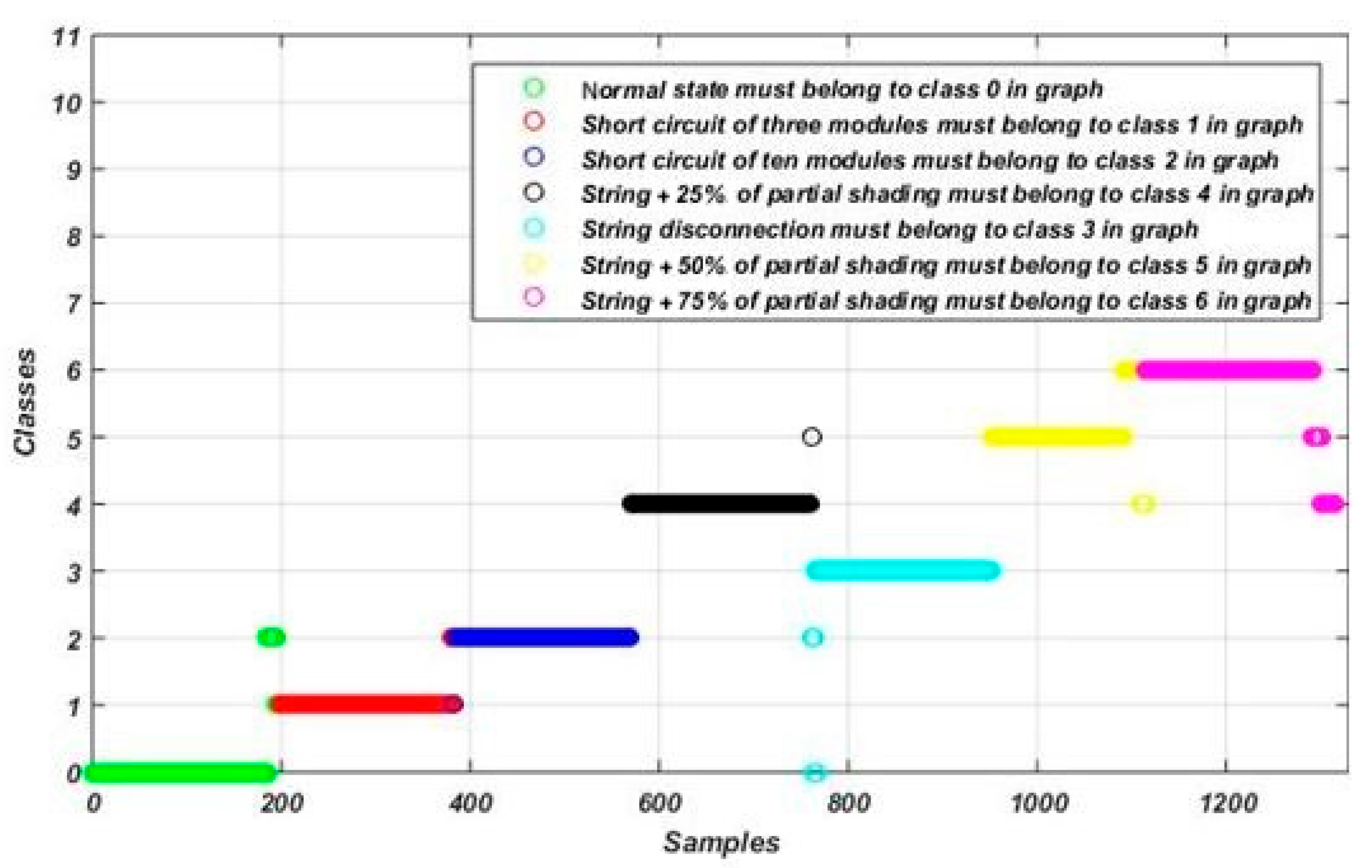
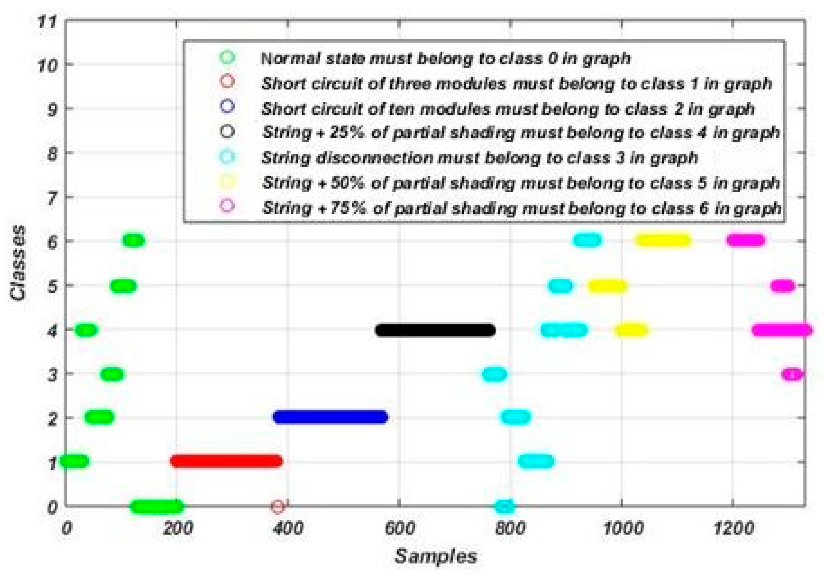
| Class Name | Label |
|---|---|
| Normal operation | Class 0 |
| Short circuit of three modules | Class 1 |
| Short circuit of ten modules | Class 2 |
| String disconnection | Class 3 |
| String disconnection with 25% of partial shading | Class 4 |
| String disconnection with 50% of partial shading | Class 5 |
| String disconnection with 75% of partial shading | Class 6 |
| Predicted Classes | ||
|---|---|---|
| Real class | Class 0 | Class 1 |
| Class 0 | TP | FN |
| Class 1 | FP | TN |
| TP | FN | FP | TN | |
|---|---|---|---|---|
| Classifier 1 | 1107 | 19 | 29 | 168 |
| Classifier 2 | 947 | 3 | 4 | 178 |
| Classifier 3 | 762 | 1 | 3 | 183 |
| Classifier 4 | 570 | 3 | 1 | 190 |
| Classifier 5 | 354 | 13 | 10 | 179 |
| Classifier 6 | 177 | 20 | 5 | 155 |
| Accuracy (%) | Precision (%) | Recall (%) | Execution Time (s) | F1-Score (%) | |
|---|---|---|---|---|---|
| Classifier 1 | 97 | 93 | 85 | 0.98 | 98 |
| Classifier 2 | 99 | 98 | 98 | 0.79 | 100 |
| Classifier 3 | 100 | 99 | 98 | 0.51 | 100 |
| Classifier 4 | 99 | 98 | 99 | 0.31 | 100 |
| Classifier 5 | 96 | 93 | 95 | 0.21 | 98 |
| Classifier 6 | 93 | 89 | 97 | 0.06 | 93 |
| Average values | 97.33 | 95 | 95.33 | 0.47 | 98.2 |
| Accuracy (%) | Precision (%) | Recall (%) | F1-Score (%) | |
|---|---|---|---|---|
| Classifier 1 | 98 | 99 | 99 | 99 |
| Classifier 2 | 99 | 100 | 100 | 100 |
| Classifier 3 | 100 | 100 | 100 | 100 |
| Classifier 4 | 100 | 100 | 100 | 100 |
| Classifier 5 | 97 | 97 | 99 | 98 |
| Classifier 6 | 96 | 97 | 96 | 96 |
| Average values | 98.33 | 99 | 99 | 99 |
| Accuracy (%) | Precision (%) | Recall (%) | F1-Score (%) | |
|---|---|---|---|---|
| Classifier 1 | 98 | 99 | 99 | 99 |
| Classifier 2 | 100 | 100 | 100 | 100 |
| Classifier 3 | 100 | 100 | 100 | 100 |
| Classifier 4 | 99 | 100 | 100 | 100 |
| Classifier 5 | 99 | 99 | 99 | 99 |
| Classifier 6 | 99 | 98 | 99 | 98 |
| Average values | 99 | 99.33 | 99.5 | 99.33 |
| SVM | DT | RF | KNN | |||||||||||||
|---|---|---|---|---|---|---|---|---|---|---|---|---|---|---|---|---|
| TP | FN | FP | TN | TP | FN | FP | TN | TP | FN | FP | TN | TP | FN | FP | TN | |
| Cl 1 | 1104 | 15 | 165 | 34 | 1113 | 6 | 23 | 176 | 1119 | 8 | 15 | 176 | 1107 | 12 | 155 | 44 |
| Cl 2 | 1086 | 0 | 122 | 61 | 950 | 3 | 3 | 180 | 950 | 1 | 1 | 180 | 1078 | 1 | 1 | 182 |
| Cl 3 | 1021 | 0 | 103 | 84 | 765 | 2 | 0 | 186 | 764 | 0 | 1 | 186 | 892 | 0 | 0 | 187 |
| Cl 4 | 927 | 0 | 107 | 90 | 566 | 3 | 0 | 196 | 568 | 1 | 0 | 196 | 696 | 0 | 0 | 196 |
| Cl 5 | 796 | 57 | 131 | 50 | 364 | 10 | 7 | 185 | 371 | 4 | 3 | 185 | 508 | 1 | 167 | 20 |
| Cl 6 | 631 | 112 | 84 | 90 | 163 | 29 | 172 | 202 | 157 | 36 | 175 | 202 | 105 | 73 | 201 | 296 |
| SVM | DT | RF | KNN | ||
|---|---|---|---|---|---|
| Classifier 1 | Accuracy (%) | 86 | 98 | 99 | 87 (K = 7) |
| Precision (%) | 87 | 98 | 99 | 88 | |
| Recall (%) | 99 | 99 | 100 | 99 | |
| F1-score (%) | 92 | 99 | 99 | 93 | |
| Execution time (s) | 0.28 | 0.02 | 0.008 | 0.21 (K = 1) | |
| Classifier 2 | Accuracy (%) | 90 | 99 | 100 | 100 |
| Precision (%) | 90 | 100 | 100 | 100 | |
| Recall (%) | 100 | 100 | 100 | 100 | |
| F1-score (%) | 93 | 91 | 100 | 100 | |
| Execution time (s) | 0.29 | 0.03 | 0.05 | 0.17 | |
| Classifier 3 | Accuracy (%) | 91 | 100 | 100 | 100 (K = 3) |
| Precision (%) | 91 | 100 | 100 | 100 | |
| Recall (%) | 100 | 100 | 100 | 100 | |
| F1-score (%) | 100 | 100 | 100 | 100 | |
| Execution time (s) | 0.05 | 0.004 | 0.07 | 0.15 | |
| Classifier 4 | Accuracy (%) | 90 | 100 | 100 | 100 (K = 2) |
| Precision (%) | 90 | 100 | 100 | 100 | |
| Recall (%) | 100 | 99 | 100 | 100 | |
| F1-score (%) | 87 | 98 | 100 | 100 | |
| Execution time (s) | 0.14 | 0.003 | 0.05 | 0.12 | |
| Classifier 5 | Accuracy (%) | 82 | 97 | 99 | 76 (K = 35) |
| Precision (%) | 86 | 98 | 99 | 75 | |
| Recall (%) | 93 | 97 | 99 | 100 | |
| F1-score (%) | 86 | 98 | 99 | 86 | |
| Execution time (s) | 0.16 | 0.003 | 0.06 | 0.11 | |
| Classifier 6 | Accuracy (%) | 78 | 64 | 63 | 59 (K = 1) |
| Precision (%) | 88 | 87 | 85 | 80 | |
| Recall (%) | 84 | 54 | 53 | 60 | |
| F1-score (%) | 51 | 78 | 65 | 68 | |
| Execution time (s) | 0.16 | 0.16 | 0.06 | 0.1 | |
| Average values | Accuracy (%) | 85.83 | 93 | 93.5 | 87 |
| Precision (%) | 88.65 | 97.16 | 97.16 | 90.5 | |
| Recall (%) | 96 | 91.50 | 92 | 93.16 | |
| F1-score (%) | 83.83 | 94 | 94 | 91.16 | |
| Execution time (s) | 0.18 | 0.006 | 0.06 | 0.14 |
| Accuracy (%) | Precision (%) | Recall (%) | Execution Time (s) | F1-Score | |
|---|---|---|---|---|---|
| The proposed algorithm | 97.33 | 98.66 | 97.5 | 0.47 | 98.2 |
| SVM | 85.33 | 88.65 | 96 | 0.18 | 83.83 |
| DT | 93 | 97.16 | 91.50 | 0.006 | 94 |
| RF | 93.50 | 97.16 | 92 | 0.06 | 94 |
| KNN | 87 | 90.50 | 93.16 | 0.14 | 91.16 |
Disclaimer/Publisher’s Note: The statements, opinions and data contained in all publications are solely those of the individual author(s) and contributor(s) and not of MDPI and/or the editor(s). MDPI and/or the editor(s) disclaim responsibility for any injury to people or property resulting from any ideas, methods, instructions or products referred to in the content. |
© 2025 by the authors. Licensee MDPI, Basel, Switzerland. This article is an open access article distributed under the terms and conditions of the Creative Commons Attribution (CC BY) license (https://creativecommons.org/licenses/by/4.0/).
Share and Cite
Mouleloued, Y.; Kara, K.; Chouder, A.; Aouaichia, A.; Silvestre, S. Euclidean Distance-Based Tree Algorithm for Fault Detection and Diagnosis in Photovoltaic Systems. Energies 2025, 18, 1773. https://doi.org/10.3390/en18071773
Mouleloued Y, Kara K, Chouder A, Aouaichia A, Silvestre S. Euclidean Distance-Based Tree Algorithm for Fault Detection and Diagnosis in Photovoltaic Systems. Energies. 2025; 18(7):1773. https://doi.org/10.3390/en18071773
Chicago/Turabian StyleMouleloued, Youssouf, Kamel Kara, Aissa Chouder, Abdelhadi Aouaichia, and Santiago Silvestre. 2025. "Euclidean Distance-Based Tree Algorithm for Fault Detection and Diagnosis in Photovoltaic Systems" Energies 18, no. 7: 1773. https://doi.org/10.3390/en18071773
APA StyleMouleloued, Y., Kara, K., Chouder, A., Aouaichia, A., & Silvestre, S. (2025). Euclidean Distance-Based Tree Algorithm for Fault Detection and Diagnosis in Photovoltaic Systems. Energies, 18(7), 1773. https://doi.org/10.3390/en18071773