Reduced-Order Modeling and Stability Analysis of Grid-Following and Grid-Forming Hybrid Renewable Energy Plants

Abstract

The control methods of energy systems can be categorized into grid-following and grid-forming types. The grid-following control method relies on grid synchronization and is prone to stability issues in weak grid conditions. By contrast, the grid-forming control method exhibits synchronous machine characteristics, providing voltage support to the system, but potentially introducing stability risks under strong grid conditions. Constructing a grid-following and grid-forming hybrid renewable energy plant can effectively enhance the system’s support capability and ensure reliable operation. However, the interactions among multiple inverters are complex, and traditional modeling methods are inadequate to meet the modeling requirements for such systems. To effectively address this problem, this paper presents a reduced-order modeling method that simplifies the complex system into a simple system consisting of an equivalent grid-following, an equivalent grid-forming, and grid impedance through frequency decoupling and the aggregation of similar inverters. Furthermore, this study employs both the Nyquist stability criterion and the harmonic characteristic analysis method to elucidate how the capacity ratio between grid-following and grid-forming affects system stability.

1. Introduction

In response to the increasing strain on conventional energy supplies and the worsening environmental crisis, the transition to low-carbon power systems is accelerating, with renewable energy playing an ever-growing role in the grid [1]. While the integration of wind, solar, and other renewable sources helps mitigate environmental issues, it also poses new challenges to the safe and stable operation of power systems [2].

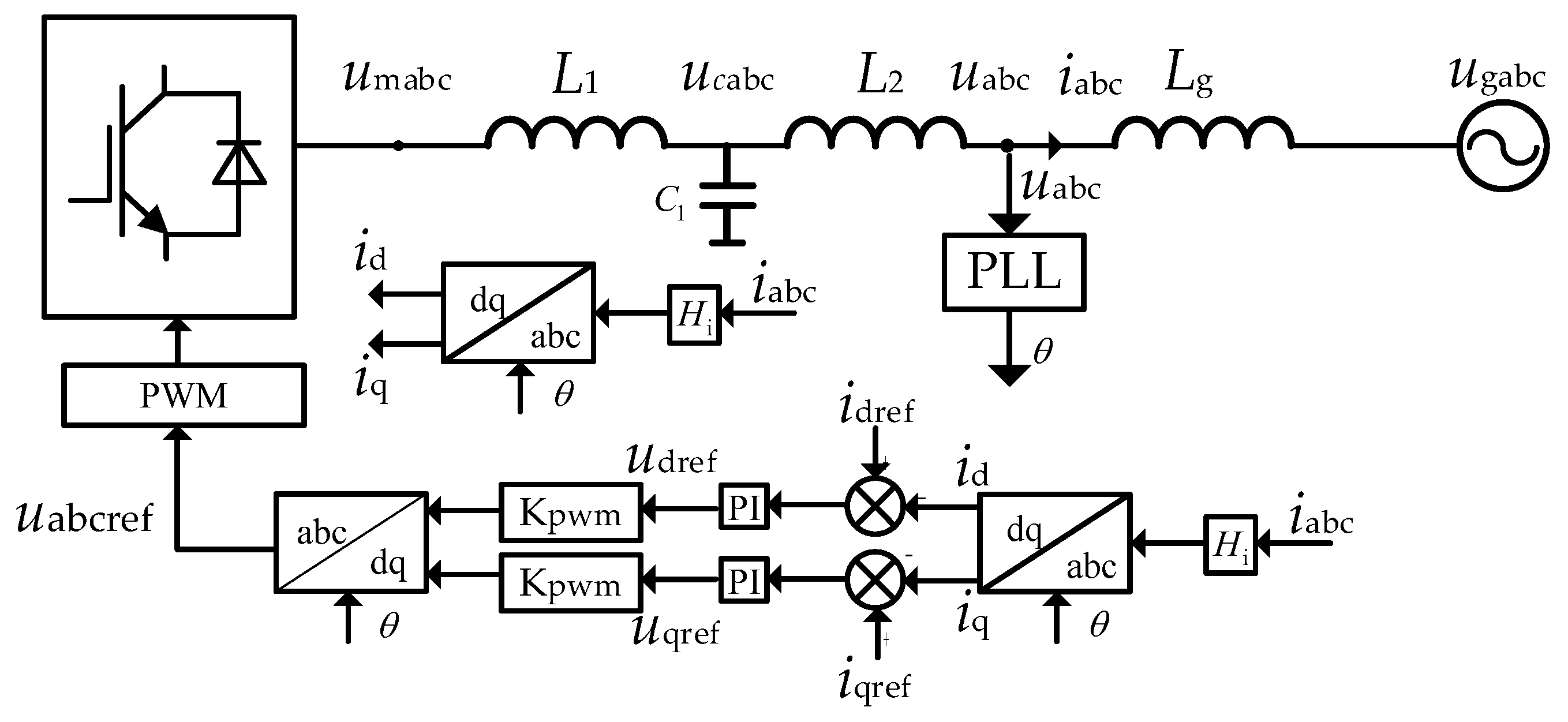
Renewable energy control methods are primarily classified into grid-following (GFL) and grid-forming (GFM) types. The GFL method synchronizes with the grid using the phase locked loop (PLL) [3] and depends on system voltage sources to maintain synchronization at the point of interconnection. 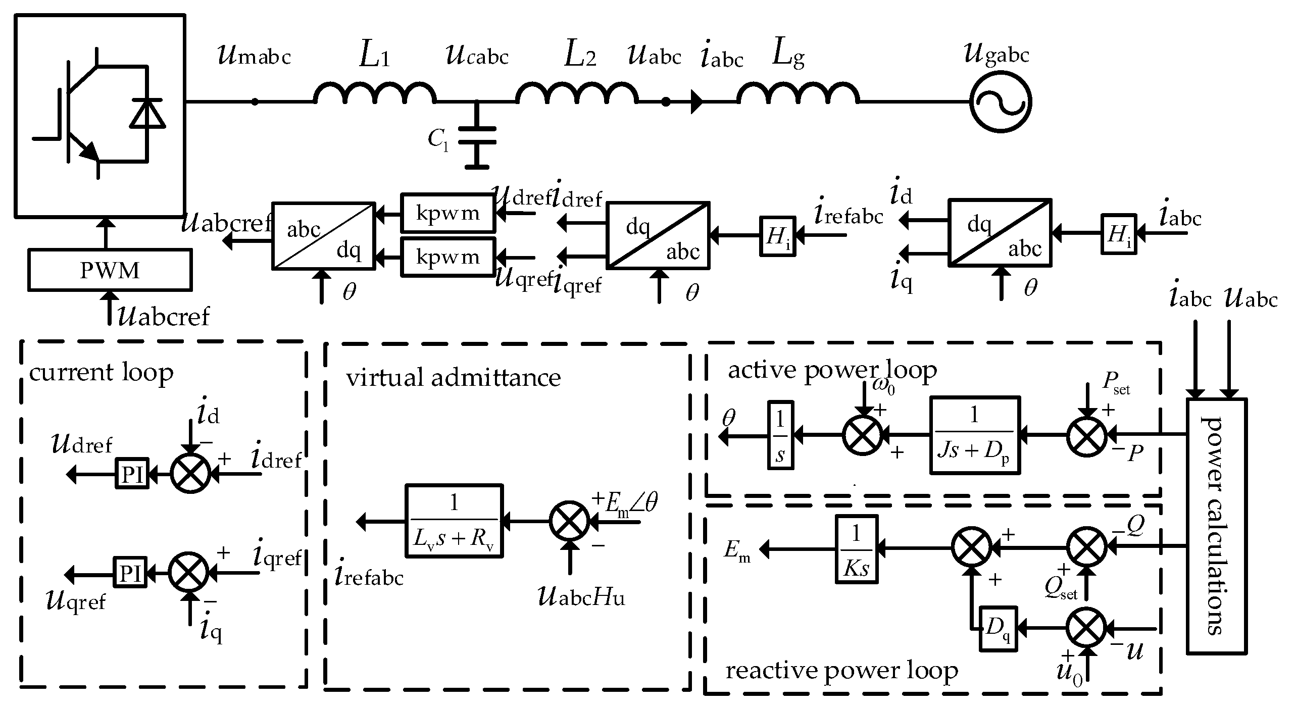However, it only passively adapts to grid conditions, offering limited support in weak grid environments, ultimately reducing system stability [4,5]. By contrast, the grid-forming (GFM) method exhibits damping and inertia characteristics similar to synchronous machines, allowing it to actively provide voltage support to the grid and maintain a higher stability margin under weak grid conditions [6,7]. However, it is prone to stability issues in strong grid environments [8]. Grid-following and grid-forming systems are suited to different grid conditions. By combining both types within a single system, the application range of inverters can be expanded, ensuring stability even when impedance fluctuates significantly due to changes in operating modes or load conditions. The hybrid application of grid-following and grid-forming can be realized through switching, integration, or hybrid control methods. The mode-switching approach automatically switches the control mode based on the detected grid impedance, though this transition may introduce unknown stability risks [9]. The control-loop integration method merges the control mechanisms of both types of inverters within the controller, which integrates their characteristics; however, this increases the difficulty of system characteristic analysis [10]. The hybrid control method, which parallels grid-following and grid-forming systems, not only improves the reliability of inverter operation but enhances flexibility in renewable energy plants [11]. The inclusion of grid-forming can resolve the issue of insufficient stability margin in grid-following renewable energy plants under weak grid conditions. In [12], the impedance characteristics of grid-following and grid-forming systems are compared using impedance modeling by Xu et al. Under weak grid conditions, the negative damping frequency range of the grid-forming system is narrower, and its amplitude characteristic is lower, compared to the grid-following system. When the two systems are hybridized, the negative damping frequency range is reduced, effectively enhancing system stability. This issue has been qualitatively explained from the perspective of a short-circuit ratio, suggesting that the grid-forming system, when modeled as a voltage source, enhances system strength and leads to an equivalent increase in the short-circuit ratio, as discussed in [13,14].

The aforementioned studies analyze the stability of grid-following and grid-forming two-machine systems through modeling. However, in renewable energy plants, multiple inverters of different types coexist. Traditional modeling methods can lead to overly complex models, making it challenging to fully capture the characteristics and interactions of each inverter. Meanwhile, neglecting certain parameters may introduce errors, reducing modeling accuracy and compromising the reliability of system analysis. In [15], Sun et al. developed a sixth-order transient model for photovoltaic-storage systems, and its stability was analyzed using the region of attraction. Nonetheless, the model’s high complexity and computational burden make it difficult to apply to renewable energy plant modeling. Some studies reduce the system order at the control level, such as Akwasi et al., who adopted new control methods for model simplification. In [16], the reduced-order Luenberger observer (ROLO) is applied to a grid-forming inverter control. The ROLO simplifies the model while preserving key dynamics and reduces computational complexity. However, as a method that removes the PI controller, it requires further experiments and validation. Meanwhile, in [17], Du et al. proposed a model reduction method for inverter-dominated microgrids by simplifying the external area model, which reduces computational complexity while preserving key dynamic responses under disturbances. However, the model includes only grid-forming inverters, without considering interactions between different types. In addition, although the dynamic performance was verified, no effective stability assessment method for multi-machine systems was provided. In [18], Rosso et al. derived the transfer function of a multi-machine system, and the stability of a grid-following and grid-forming hybrid system was evaluated using the μ analysis method. This approach, based on multivariable control theory, facilitates the assessment of robust stability under various conditions. The lack of a clear physical interpretation, however, limits the ability to conduct further mechanism analysis of the system. In [19], a hybrid system support index was introduced by Wang et al. to address the qualitative stability analysis of renewable energy plants, characterizing the stability of hybrid systems. The inclusion of a grid-forming inverter adds a polynomial with positive coefficients to both the hybrid short-circuit ratio and the support index. Nevertheless, the calculation of these indicators depends on accurate system parameters, their general applicability and adaptability still need further verification. In [20], an impedance-based composite grid modeling method was proposed to construct the admittance matrix of a renewable energy plant with multiple inverters. The system’s stability was determined using eigenvalue analysis. This approach, though, ignores the interactions between inverters, which compromises the accuracy of the model. Additionally, solving the eigenvalues of high-order matrices is a challenging task, adding complexity to the method. In [21], a model reduction method for grid-forming inverters based on frequency-domain perturbation operators is presented. It simplifies stability analysis and effectively identifies factors affecting single-machine impedance. However, the method is not extended to renewable energy plants. Overall, the existing modeling methods are relatively complex and fail to account for the interactions between inverters, making it difficult to accurately reflect the impedance characteristics of grid-following and grid-forming hybrid renewable energy plants.

In a nutshell, this paper addresses the issues of high complexity and low versatility in existing modeling methods for renewable energy plants by constructing reduced-order models for grid-following and grid-forming hybrid renewable energy plants. It also explores the capacity ratio problem of two types of inverters in these plants from the perspectives of the harmonic suppression using the Nyquist stability criterion and harmonic analysis methods. Additionally, the conclusions drawn from the analysis are validated through simulation. Finally, the research findings of this paper are summarized.

2. Topology and Control Block Diagram of Grid-Following and Grid-Forming Hybrid Renewable Energy Plants

This section presents the hybrid system topology and control block diagrams for both grid-following and grid-forming inverters. The grid-following inverter uses a phase-locked loop to measure the point of common coupling, employing closed-loop control to synchronize with the grid’s voltage and frequency. The grid-forming inverter, on the other hand, actively controls system frequency and voltage. In weak grid environments, it mimics synchronous machine behavior, providing inertia and damping support to maintain system stability.

2.1. Topology of Renewable Energy Plant

The capacity of renewable energy plants typically ranges from 100 MW to 1000 MW, significantly larger than single-machine systems, and the greater number of inverters further increases modeling complexity. As technology advances, grid-following and grid-forming hybrid renewable energy plants have emerged, enabling stable operation under varying short-circuit ratios. However, the complex interactions among inverters pose additional challenges for modeling and stability analysis. Figure 1 illustrates the topology of a grid-following and grid-forming hybrid renewable energy plant, comprising converter groups, transformers, transmission lines, and an AC power grid.

In renewable energy plants, inverters convert direct current power into alternating current power, which is more suitable for transmission. Grid-following and grid-forming hybrid renewable energy plants incorporate both grid-following inverters and grid-forming inverters. Grid-following inverters perform well and maintain good stability in strong power grids, while grid-forming inverters provide better stability under weak power grid conditions. By combining the advantages of both types of inverters, such hybrid renewable energy plants can achieve stable operation even when the short-circuit ratio of the power grid changes. The following study focuses on the modeling and stability analysis of this type of inverter.

2.2. Control Structure of Grid-Following/Grid-Forming Inverter

The control block diagrams for grid-following and grid-forming systems are shown in Figure 2 and Figure 3. The grid-following inverter utilizes a phase-locked loop (PLL) to achieve synchronization by detecting the grid phase. In Figure 2, L₁, L₂, and C₁ represent the filter inductors and capacitors, L_g is the grid inductance, u_abc is the port voltage, i_abc is the port current, i_dref and i_qref are the reference values for the d-axis and q-axis currents, u_dref and u_qref are the reference values for the d-axis and q-axis voltages.

The grid-forming inverter uses virtual synchronous generator control (VSG), as shown in Figure 3. In this diagram, L₁, L₂, and C₁ represent the filter inductors and capacitors; u_mabc is the bridge arm voltage; u_abc is the grid connection point voltage; i_abc is the grid connection point current; P_set and Q_set are the rated active and reactive powers; P and Q represent the active and reactive power generated by GFM; J represents inertia; D_p and D_q are the active and reactive damping coefficients; u and u₀ are the rated voltage RMS value and the output voltage RMS value; K is the reactive inertia coefficient; θ and E_m are the output power angle and output voltage RMS value of the VSG; L_v and R_v are the virtual inductance and virtual resistance, which together form the virtual admittance. The control loop consists of active power, reactive power, virtual admittance, and current loops.

3. Reduced-Order Modeling Method for Grid-Following and Grid-Forming Hybrid Renewable Energy Plants

The grid-following and grid-forming hybrid renewable energy plant represents a promising solution that aligns with the current trends in energy development. However, conventional modeling methods are often complicated, lack general applicability, and are difficult to adapt to the stability analysis requirements of such hybrid systems. To overcome these limitations, this paper proposes a model order reduction method tailored for grid-following and grid-forming hybrid renewable energy plants. The equivalent admittance matrices of the grid-following and grid-forming inverters are derived, and the accuracy of the proposed model is verified through comparison between calculated and measured results.

3.1. Modeling of Grid-Following/Grid-Forming Inverters

The impedance method is based on harmonic linearization theory [22]. By injecting a harmonic signal into the terminal voltage and measuring the corresponding harmonic current at the grid connection point, the system’s impedance model can be derived. In the grid-following and grid-forming hybrid renewable energy plant, transformers and transmission lines result in phase angle discrepancies between the terminal voltages of different types of inverters. Therefore, when calculating the impedance models for grid-following and grid-forming inverters, it is essential to account for the phase of their respective terminal voltages. Frequency coupling effects exist in both grid-following and grid-forming inverters. When a positive-sequence voltage with frequency f_p is injected at the grid connection point, it generates a positive-sequence current component at f_p and a negative-sequence current component at f_p-2f₁ [23]. Taking the grid-forming inverter as an example, when a positive-sequence disturbance signal is injected into phase-a of the terminal voltage, the time-domain expressions for the voltage and current are as follows:

$$\begin{array}{l}{u}_{\mathrm{a}}(t)=U_1\cos (2\mathrm{\pi }{f}_{1}t+{\mathrm{\phi }}_{\mathrm{u}})+U_{\mathrm{p}}\cos (2\mathrm{\pi }{f}_{\mathrm{p}}t+{\mathrm{\phi }}_{\mathrm{up}})+U_{\mathrm{n}}\cos (2\mathrm{\pi }{f}_{\mathrm{n}}t+{\mathrm{\phi }}_{\mathrm{un}})\\ i_{\mathrm{a}}(t)=I_1\cos (2\mathrm{\pi }{f}_{1}t+{\mathrm{\phi }}_{\mathrm{i}})+I_{\mathrm{p}}\cos (2\mathrm{\pi }{f}_{\mathrm{p}}t+{\mathrm{\phi }}_{\mathrm{ip}})+I_{\mathrm{n}}\cos (2\mathrm{\pi }{f}_{\mathrm{n}}t+{\mathrm{\phi }}_{\mathrm{in}})\end{array}$$

(1)

The above expressions are transformed into the frequency domain, and the expressions are as follows:

$$\begin{array}{l}{u}_{\mathrm{a}}=\left\{\begin{array}{l}{\mathit{U}}_1,\begin{array}{cc}\hspace{1em}\hspace{1em}& f=\pm f_1\end{array}\\ {\mathit{U}}_{\mathrm{p}},\begin{array}{cc}\hspace{1em}\hspace{1em}& f=\pm f_{\mathrm{p}}\end{array}\end{array}\right.\\ i_{\mathrm{a}}=\left\{\begin{array}{l}{\mathit{I}}_1,\begin{array}{cc}\hspace{1em}\hspace{1em}& f=\pm f_1\end{array}\\ {\mathit{I}}_{\mathrm{p}},\begin{array}{cc}\hspace{1em}\hspace{1em}& f=\pm f_{\mathrm{p}}\end{array}\\ {\mathit{I}}_{\mathrm{n}},\begin{array}{cc}\hspace{1em}\hspace{1em}& \hfill f=\pm (f_{\mathrm{p}}-2f_1)\end{array}\end{array}\right.\end{array}$$

(2)

In Equation (2), ${\mathit{U}}_1=({\mathit{U}}_1/2){\mathrm{e}}^{\pm \mathrm{j}{\mathit{\phi }}_{\mathrm{u}}}$, ${\mathit{U}}_{\mathrm{p}}=({\mathit{U}}_{\mathrm{p}}/2){\mathrm{e}}^{\pm \mathrm{j}{\mathit{\phi }}_{\mathrm{up}}}$, ${\mathit{I}}_1=({\mathit{I}}_1/2){\mathrm{e}}^{\pm \mathrm{j}{\mathit{\phi }}_{\mathrm{i}}}$, ${\mathit{I}}_{\mathrm{p}}=({\mathit{I}}_{\mathrm{p}}/2){\mathrm{e}}^{\pm \mathrm{j}{\mathit{\phi }}_{\mathrm{ip}}}$ and ${\mathit{I}}_{\mathrm{n}}=({\mathit{I}}_{\mathrm{n}}/2){\mathrm{e}}^{\pm \mathrm{j}{\mathit{\phi }}_{\mathrm{in}}}$; U₁, U_p represent the fundamental voltage and the amplitude of the positive-sequence disturbance voltage; I₁, I_p, I_n represent the amplitudes of the fundamental current, positive-sequence disturbance current, and negative-sequence disturbance current; φ_u represents the initial phase angle of the fundamental voltage; φ_up represents the initial phase angle of the disturbance voltage; φ_i represents the initial phase angle of fundamental current; φ_ip and φ_in represent the initial phase angles of the positive-sequence disturbance current and the negative-sequence disturbance current. Based on the control block diagrams of grid-following and grid-forming inverters, the admittance models incorporating the terminal voltage phase angle can be derived as follows:

$$\left[\begin{array}{c}{U}_{\mathrm{p}\_\mathrm{GFL}}(s)\\ U_{n\_\mathrm{GFL}}(s)\end{array}\right]=\left[\begin{array}{cc}{Y}_{11\_\mathrm{GFL}}(s)& Y_{21\_\mathrm{GFL}}(s)\\ Y_{12\_\mathrm{GFL}}(s)& Y_{22\_\mathrm{GFL}}(s)\end{array}\right]\left[\begin{array}{c}{I}_{\mathrm{p}\_\mathrm{GFL}}(s)\\ I_{n\_\mathrm{GFL}}(s)\end{array}\right]$$

(3)

$$\left[\begin{array}{c}{U}_{\mathrm{p}\_\mathrm{GFM}}(s)\\ U_{\mathrm{n}\_\mathrm{GFM}}(s)\end{array}\right]=\left[\begin{array}{cc}{Y}_{11\_\mathrm{GFM}}(s)& Y_{21\_\mathrm{GFM}}(s)\\ Y_{12\_\mathrm{GFM}}(s)& Y_{22\_\mathrm{GFM}}(s)\end{array}\right]\left[\begin{array}{c}{I}_{\mathrm{p}\_\mathrm{GFM}}(s)\\ I_{\mathrm{n}\_\mathrm{GFM}}(s)\end{array}\right]$$

(4)

In Equation (3), Y_{11_GFL}(s), Y_{21_GFL}(s), Y_{22_GFL}(s), and Y_{12_GFL}(s) represent the impedance expressions for the grid-following inverter, as detailed in Appendix A, Equations (A2)–(A5). Similarly, in Equation (4), Y_{11_GFM}(s), Y_{21_GFM}(s), Y_{22_GFM}(s), and Y_{12_GFM}(s) correspond to the impedance expressions for the grid-forming inverter, provided in Appendix A, Equations (A14)–(A17).

3.2. Overview of Reduced-Order Modeling Methods

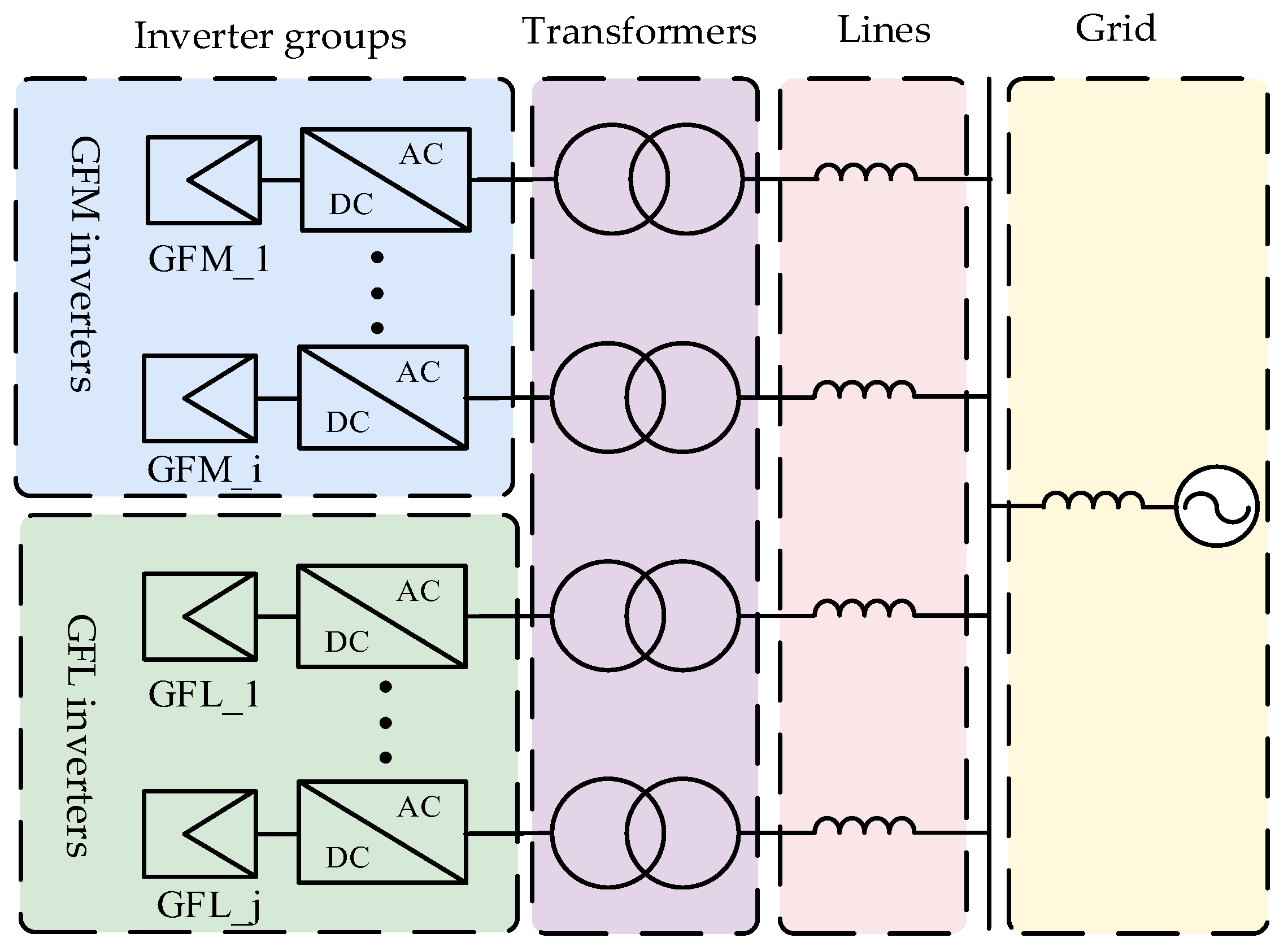
The grid-following and grid-forming hybrid renewable energy plant is a highly complex system. If the entire plant is modeled directly, the model complexity becomes extremely high, as shown in [24], and you would need to spend a significant amount of time handling this complex matrix, which could even lead to a dimensional explosion. In the topology shown in Figure 1, directly modeling a grid-following and grid-forming hybrid renewable energy plant with i grid-forming inverters and j grid-following inverters results in an impedance model of order (2i + 2j) × (2i + 2j), as given in Equation (5). As i and j increase, the difficulty of analyzing the impedance model rises significantly. Therefore, reducing the model order is essential to simplify the analysis of impedance characteristics.

$$\left[\begin{array}{c}\begin{array}{l}{U}_{\mathrm{p}\_\mathrm{GFM}1}(s)\\ U_{n\_\mathrm{GFM}1}(s)\\ \dots \\ U_{\mathrm{p}\_\mathrm{GFLj}}(s)\\ U_{n\_\mathrm{GFLj}}(s)\end{array}\end{array}\right]=\left[\begin{array}{ccccc}{Y}_{11\_\mathrm{GFM}1}(s)& Y_{21\_\mathrm{GFM}1}(s)& & & \\ Y_{12\_\mathrm{GFM}1}(s)& Y_{22\_\mathrm{GFM}1}(s)& & & \\ & & \dots & & \\ & & & Y_{11\_\mathrm{GFLj}}(s)& Y_{11\_\mathrm{GFLj}}(s)\\ & & & Y_{11\_\mathrm{GFLj}}(s)& Y_{11\_\mathrm{GFLj}}(s)\end{array}\right]\left[\begin{array}{c}\begin{array}{l}{I}_{\mathrm{p}\_\mathrm{GFM}1}(s)\\ I_{\mathrm{n}\_\mathrm{GFM}1}(s)\\ \dots \\ I_{\mathrm{p}\_\mathrm{GFLj}}(s)\\ I_{\mathrm{n}\_\mathrm{GFLj}}(s)\end{array}\end{array}\right]$$

(5)

During the plant modeling process, if the impedance of inverters and transformers is known, their series and parallel connections can be determined based on their electrical interconnections, ultimately establishing the impedance model of the grid-following and grid-forming hybrid renewable energy plant. As shown in Equation (5), the admittance matrix of inverters contains coupling terms. When inverters are connected in series with transformers and transmission lines, coupling effects alter the impedance of both the inverters and the lines. These changes also occur between inverters and the grid. Neglecting such effects will introduce errors in the impedance matrix, affecting the accuracy of stability analysis.

Based on the above analysis, implementing an appropriate model order reduction in the modeling process of grid-following and grid-forming hybrid renewable energy plants can significantly simplify the impedance model. At the same time, considering the coupling effects between inverters and other components helps maintain the accuracy of the modeling results.

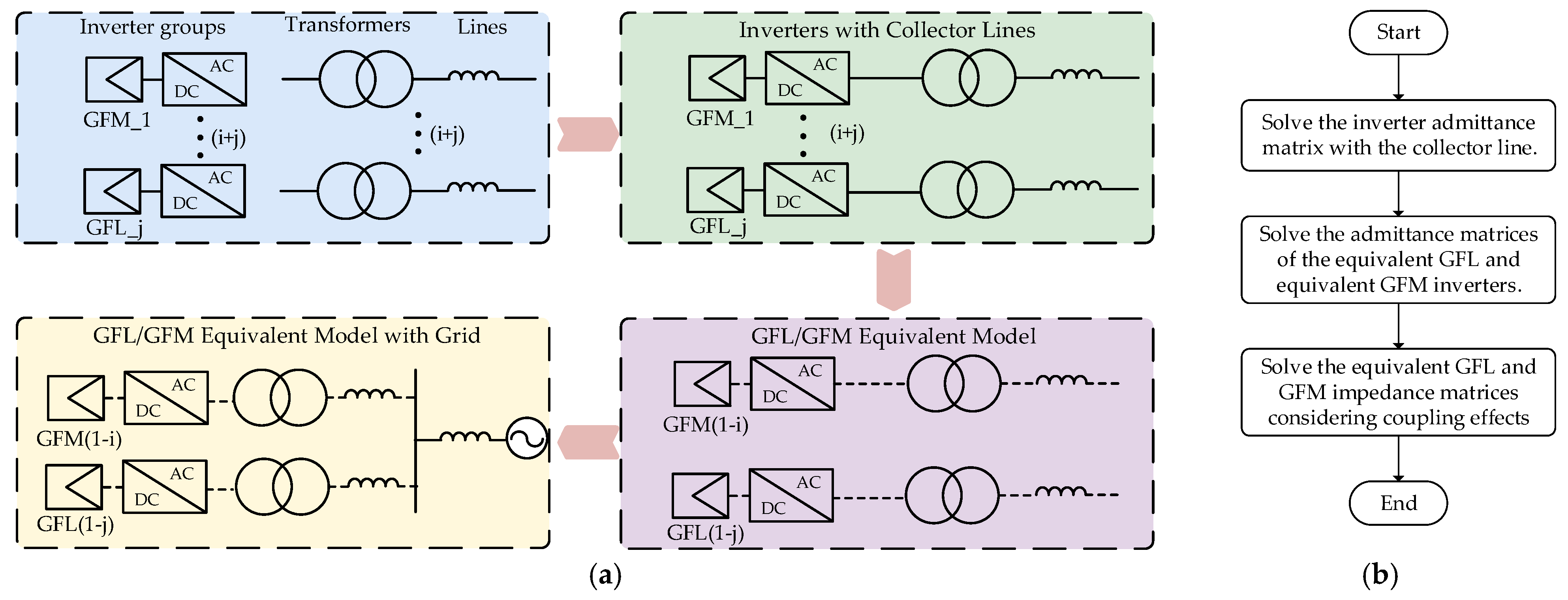
The flowchart of the reduced-order modeling method is shown in Figure 4. First, based on the impedance models of grid-following/grid-forming inverters, transformers, and transmission lines, the admittance model of inverters with collector lines is derived, while also taking into account the coupling effects between the inverters and the transmission lines. Next, inverters of the same type are categorized and aggregated to obtain the equivalent admittance matrices for grid-following and grid-forming inverters. Finally, the system is connected to the grid, and the equivalent admittance matrices for grid-following and grid-forming inverters are derived, while considering frequency coupling effects both among inverters and between inverters and the grid. This model reduction approach maintains accuracy, while simplifying the renewable energy plant into a simple circuit, where the equivalent grid-following and grid-forming inverters operate in parallel with the power grid. The following sections provide a detailed analysis of this model reduction approach based on specific system models.

3.3. Detailed Description of Reduced-Order Modeling Methods

Referring to the flowchart in Figure 4, the first step is to calculate the admittance matrix of inverters with the collection line. As shown in Figure 5, when the inverter is in series with the line, the coupled current flows through the collection line, creating a current loop. The collection line impedance affects the inverter’s admittance, so it is essential to account for these coupling effects during the derivation to ensure the accuracy of the results.

In Figure 5, Y_{11_1}(s), Y_{12_1}(s), Y_{22_1}(s), and Y_{21_1}(s) represent the admittance matrix of the inverter in an ideal grid system, while Z_Ls(s) is the sum of the line impedance and transformer impedance. According to Ohm’s law, Y = U/I, the admittance matrix of the inverter operating in stand-alone mode is given by the following:

$$\begin{array}{l}{Y}_{11\_1}(s)=-{\displaystyle \frac{i_{\mathrm{p}1\_1}(s)}{u_{\mathrm{p}}(s)}}\\ Y_{21\_1}(s)=-{\displaystyle \frac{i_{\mathrm{n}2\_1}(s)}{u_{\mathrm{p}}(s)}}\\ Y_{22\_1}(s)=-{\displaystyle \frac{i_{\mathrm{n}1\_1}(s)}{u_{\mathrm{n}}(s)}}\\ Y_{12\_1}(s)=-{\displaystyle \frac{i_{\mathrm{p}2\_1}(s)}{u_{\mathrm{n}}(s)}}\end{array}$$

(6)

After the collector lines are integrated, the coupling paths within the system are modified. The admittance matrix of the inverter with collection line is as follows:

$$\begin{array}{l}{Y}_{11\_\mathrm{coupling}}(s)=-{\displaystyle \frac{i_{\mathrm{p}\_1}(s)}{u_{\mathrm{p}}(s)}}\\ Y_{21\_\mathrm{coupling}}(s)=-{\displaystyle \frac{i_{\mathrm{n}\_1}(s)}{u_{\mathrm{p}}(s)}}\\ Y_{22\_\mathrm{coupling}}(s)=-{\displaystyle \frac{i_{\mathrm{n}\_1}(s)}{u_{\mathrm{n}}(s)}}\\ Y_{12\_\mathrm{coupling}}(s)=-{\displaystyle \frac{i_{\mathrm{p}\_1}(s)}{u_{\mathrm{n}}(s)}}\end{array}$$

(7)

Based on the relationships shown in Figure 5 and Ohm’s law, I = U × Y, the relationship between current and voltage can be expressed as follows:

$$\begin{array}{l}{i}_{\mathrm{p}1\_1}(s)=-u_{\mathrm{p}}(s)Y_{11\_1}(s)\\ i_{\mathrm{p}2\_1}(s)=-u_{\mathrm{n}}(s)Y_{12\_1}(s-2j\omega )\\ i_{\mathrm{n}1\_1}(s)=-u_{\mathrm{p}}(s)Y_{21\_1}(s)\\ i_{\mathrm{n}2\_1}(s)=-u_{\mathrm{n}}(s)Y_{22\_1}(s-2j\omega )\\ u_{\mathrm{p}}(s)=Z_{\mathrm{Ls}}(s)[i_{\mathrm{p}1\_1}(s)+i_{\mathrm{p}2\_1}(s)]\\ u_{\mathrm{n}}(s)=Z_{\mathrm{Ls}}(s-2j\omega )[i_{\mathrm{p}1\_1}(s)+i_{\mathrm{p}2\_1}(s)]\end{array}$$

(8)

Based on Equation (8), the inverter admittance matrix considering frequency coupling can be obtained through the following calculation:

$$\begin{array}{l}{Y}_{11\_\mathrm{coupling}}(s)=Y_{11}(s)-{\displaystyle \frac{Y_{12\_1}(s-2\mathrm{j}\omega )Y_{21\_1}(s)}{Y_{\mathrm{Ls}}(s-2\mathrm{j}\omega )+Y_{22\_1}(s-2\mathrm{j}\omega )}}\\ Y_{21\_\mathrm{coupling}}(s)=Y_{21}(s)-{\displaystyle \frac{Y_{22\_1}(s-2\mathrm{j}\omega )Y_{21\_1}(s)}{Y_{\mathrm{Ls}}(s-2\mathrm{j}\omega )+Y_{22\_1}(s-2\mathrm{j}\omega )}}\\ Y_{22\_\mathrm{coupling}}(s)=Y_{22}(s)-{\displaystyle \frac{Y_{21\_1}(s+2\mathrm{j}\omega )Y_{12\_1}(s)}{Y_{\mathrm{Ls}}(s+2\mathrm{j}\omega )+Y_{11\_1}(s+2\mathrm{j}\omega )}}\\ Y_{12\_\mathrm{coupling}}(s)=Y_{12}(s)-{\displaystyle \frac{Y_{11\_1}(s+2\mathrm{j}\omega )Y_{12\_1}(s)}{Y_{\mathrm{Ls}}(s+2\mathrm{j}\omega )+Y_{11\_1}(s+2\mathrm{j}\omega )}}\end{array}$$

(9)

In Equation (9), Y_{11_coupling}(s), Y_{21_coupling}(s), Y_{22_coupling}(s), and Y_{12_coupling}(s) denote the inverter admittance matrix considering frequency coupling. The admittance matrix of the collection line incorporating these coupling effects can be expressed as follows:

$$\begin{array}{l}{Y}_{11\_\mathrm{Lscoupling}}(s)=Y_{\mathrm{Ls}}(s)\\ Y_{21\_\mathrm{Lscoupling}}(s)={\displaystyle \frac{Y_{21\_\mathrm{coupling}}(s)}{Y_{11\_\mathrm{coupling}}(s)}}{Y}_{\mathrm{Ls}}(s)\\ Y_{22\_\mathrm{Lscoupling}}(s)=Y_{\mathrm{Ls}}(s)\\ Y_{12\_\mathrm{Lscoupling}}(s)={\displaystyle \frac{Y_{12\_\mathrm{coupling}}(s)}{Y_{22\_\mathrm{coupling}}(s)}}{Y}_{\mathrm{Ls}}(s)\end{array}$$

(10)

In Equation (10), Y_{11_Lscoupling}(s), Y_{21_Lscoupling}(s), Y_{22_Lscoupling}(s), and Y_{12_Lscoupling}(s) denote the collection line admittance matrix considering frequency coupling. Since the inverter and collection line impedance are in series, the admittance is given by Y_equ(s) = Y_Lscoupling(s) × Y_coupling(s)/[Y_Lscoupling(s) + Y_coupling(s)]. The admittance matrix for the series combination of the collection line and inverter can be derived from Equations (9) and (10), as follows:

$$\begin{array}{l}{Y}_{11\mathrm{equ}}(s)={\displaystyle \frac{[Z_{\mathrm{Ls}}(s-2\mathrm{j}\omega )Y_{11\_1}(s)Y_{22\_1}(s-2\mathrm{j}\omega )+Y_{11\_1}(s)-Z_{\mathrm{Ls}}(s)(s-2\mathrm{j}\omega )Y_{12\_1}(s-2\mathrm{j}\omega )Y_{21\_1}(s)]}{[1+Y_{22\_1}(s-2\mathrm{j}\omega )Z_{\mathrm{Ls}}(s-2\mathrm{j}\omega )+Z_{\mathrm{Ls}}(s)Y_{11\_1}(s)+Z_{\mathrm{Ls}}(s-2\mathrm{j}\omega )Z_{\mathrm{Ls}}(s)Y_{11\_1}(s)Y_{22\_1}(s-2\mathrm{j}\omega )-Y_{12\_1}(s-2\mathrm{j}\omega )Y_{21\_1}(s)Z_{\mathrm{Ls}}(s-2\mathrm{j}\omega )Z_{\mathrm{Ls}}(s)]}}\\ Y_{21\mathrm{equ}}(s)={\displaystyle \frac{Y_{21\_1}(s)}{[1+Y_{22\_1}(s-2\mathrm{j}\omega )Z_{\mathrm{Ls}}(s-2\mathrm{j}\omega )+Z_{\mathrm{Ls}}(s)Y_{11\_1}(s)+Z_{\mathrm{equ}}(s-2\mathrm{j}\omega )Z_{\mathrm{Ls}}(s)Y_{11\_1}(s)Y_{22\_1}(s-2\mathrm{j}\omega )-Y_{12\_1}(s-2\mathrm{j}\omega )Y_{21\_1}(s)Z_{\mathrm{Ls}}(s-2\mathrm{j}\omega )Z_{\mathrm{Ls}}(s)]}}\\ Y_{12\mathrm{equ}}(s)={\displaystyle \frac{Y_{12\_1}(s)}{[1+Y_{11\_1}(s+2\mathrm{j}\omega )Z_{\mathrm{Ls}}(s+2\mathrm{j}\omega )+Z_{\mathrm{Ls}}(s)Y_{22\_1}(s)+Y_{22\_1}(s)Z_{\mathrm{Ls}}(s+2\mathrm{j}\omega )Z_{\mathrm{Ls}}(s)Y_{11\_1}(s+2\mathrm{j}\omega )-Y_{21\_1}(s+2\mathrm{j}\omega )Z_{\mathrm{Ls}}(s+2\mathrm{j}\omega )Y_{12\_1}(s)Z_{\mathrm{Ls}}(s)]}}\\ Y_{22\mathrm{equ}}(s)={\displaystyle \frac{[Z_{\mathrm{Ls}}(s+2\mathrm{j}\omega )Y_{22\_1}(s)Y_{11\_1}(s+2\mathrm{j}\omega )+Y_{22\_1}(s)-Z_{\mathrm{Ls}}(s+2\mathrm{j}\omega )Y_{21\_1}(s+2\mathrm{j}\omega )Y_{12\_1}(s)]}{[1+Y_{11\_1}(s+2\mathrm{j}\omega )Z_{\mathrm{Ls}}(s+2\mathrm{j}\omega )+Z_{\mathrm{Ls}}(s)Y_{22\_1}(s)+Y_{22\_1}(s)Z_{\mathrm{Ls}}(s+2\mathrm{j}\omega )Z_{\mathrm{Ls}}(s)Y_{11\_1}(s+2\mathrm{j}\omega )-Y_{21\_1}(s+2\mathrm{j}\omega )Z_{\mathrm{Ls}}(s+2\mathrm{j}\omega )Y_{12\_1}(s)Z_{\mathrm{Ls}}(s)]}}\end{array}$$

(11)

In the Equation (11), Y_11equ(s), Y_12equ(s), Y_21equ(s), and Y_22equ(s) represent the admittance matrix of the inverter with the collection line.

According to the flowchart in Figure 4, after deriving the inverter admittance matrix with the collection line, the system can be simplified to multiple parallel inverters connected in series with the grid. In the plant, inverters are categorized into grid-following and grid-forming based on their control methods. Aggregating inverters with the same control method helps reduce the order of the admittance matrix. However, coupling effects exist both among inverters and between inverters and the power grid. Therefore, these coupling effects should be considered when deriving the equivalent grid-following and grid-forming admittances. Figure 6 illustrates the coupling relationships between positive and negative sequence voltages, as well as their corresponding currents in the renewable energy plant.

In Figure 6, Z_g(s) represents the power grid impedance matrix, while Y_11equk(s), Y_21equk(s), Y_22equk(s), and Y_12equk(s) denote the admittance matrices of inverters with the collection lines. The voltage and current of each inverter in the coupling loop are related as follows:

$$\begin{array}{l}{i}_{\mathrm{p}1\_\mathrm{equGFM}1}(s)=-u_{\mathrm{p}}(s)Y_{11\_\mathrm{equGFM}1}(s)\\ i_{\mathrm{p}2\_\mathrm{equGFM}1}(s)=-u_{\mathrm{n}}(s)Y_{12\_\mathrm{equGFM}1}(s-2\mathrm{j}\omega )\\ i_{\mathrm{n}1\_\mathrm{equGFM}1}(s)=-u_{\mathrm{p}}(s)Y_{21\_\mathrm{equGFM}1}(s)\\ i_{\mathrm{n}2\_\mathrm{equGFM}1}(s)=-u_{\mathrm{n}}(s)Y_{22\_\mathrm{equGFM}1}(s-2\mathrm{j}\omega )\\ \\ i_{\mathrm{p}1\_\mathrm{equGFLj}}(s)=-u_{\mathrm{p}}(s)Y_{11\_\mathrm{equGFLj}}(s)\\ i_{\mathrm{p}2\_\mathrm{equGFLj}}(s)=-u_{\mathrm{n}}(s)Y_{12\_\mathrm{equGFLj}}(s-2\mathrm{j}\omega )\\ i_{\mathrm{n}1\_\mathrm{equGFLj}}(s)=-u_{\mathrm{p}}(s)Y_{21\_\mathrm{equGFLj}}(s)\\ i_{\mathrm{n}2\_\mathrm{equGFLj}}(s)=-u_{\mathrm{n}}(s)Y_{22\_\mathrm{equGFLj}}(s-2\mathrm{j}\omega )\end{array}$$

(12)

By aggregating inverters of the same type, their admittances are summed, yielding the following:

$${\displaystyle \sum _{k=1}^i{i}_{\mathrm{p}1\_\mathrm{equGFMk}}(s)}=-u_{\mathrm{p}}(s){\displaystyle \sum _{k=1}^i{Y}_{11\_\mathrm{equGFMk}}(s)}$$

$${\displaystyle \sum _{k=1}^i{i}_{\mathrm{p}2\_\mathrm{equGFMk}}(s)}=-u_{\mathrm{n}}(s){\displaystyle \sum _{k=1}^i{Y}_{12\_\mathrm{equGFMk}}(s-2\mathrm{j}\omega )}$$

$${\displaystyle \sum _{k=1}^i{i}_{\mathrm{n}1\_\mathrm{equGFMk}}(s)}=-u_{\mathrm{p}}(s){\displaystyle \sum _{k=1}^i{Y}_{21\_\mathrm{equGFMk}}(s)}$$

$${\displaystyle \sum _{k=1}^i{i}_{\mathrm{n}2\_\mathrm{equGFMk}}(s)}=-u_{\mathrm{n}}(s){\displaystyle \sum _{k=1}^i{Y}_{22\_\mathrm{equGFMk}}(s-2\mathrm{j}\omega )}$$

$${\displaystyle \sum _{k=1}^j{i}_{\mathrm{p}1\_\mathrm{equGFLk}}(s)}=-u_{\mathrm{p}}(s){\displaystyle \sum _{k=1}^j{Y}_{11\_\mathrm{equGFLk}}(s)}$$

$${\displaystyle \sum _{k=1}^j{i}_{\mathrm{p}2\_\mathrm{equGFLk}}(s)}=-u_{\mathrm{n}}(s){\displaystyle \sum _{k=1}^j{Y}_{12\_\mathrm{equGFLk}}(s-2\mathrm{j}\omega )}$$

$${\displaystyle \sum _{k=1}^j{i}_{\mathrm{n}1\_\mathrm{equGFLk}}(s)}=-u_{\mathrm{p}}(s){\displaystyle \sum _{k=1}^j{Y}_{21\_\mathrm{equGFLk}}(s)}$$

$${\displaystyle \sum _{k=1}^j{i}_{\mathrm{n}2\_\mathrm{equGFLk}}(s)}=-u_{\mathrm{n}}(s){\displaystyle \sum _{k=1}^j{Y}_{22\_\mathrm{equGFLk}}(s-2\mathrm{j}\omega )}$$

$$u_{\mathrm{p}}(s)=Z_{\mathrm{g}}(s)[{\displaystyle \sum _{k=1}^i{i}_{\mathrm{p}1\_\mathrm{equGFMk}}(s)}+{\displaystyle \sum _{k=1}^i{i}_{\mathrm{p}2\_\mathrm{equGFMk}}(s)}+{\displaystyle \sum _{k=1}^j{i}_{\mathrm{p}1\_\mathrm{equGFLk}}(s)}+{\displaystyle \sum _{k=1}^j{i}_{\mathrm{p}2\_\mathrm{equGFLk}}(s)}]$$

$$u_{\mathrm{n}}(s)=Z_{\mathrm{g}}(s-2\mathrm{j}\omega )[{\displaystyle \sum _{k=1}^i{i}_{\mathrm{n}1\_\mathrm{equGFMk}}(s)}+{\displaystyle \sum _{k=1}^i{i}_{\mathrm{n}2\_\mathrm{equGFMk}}(s)}+{\displaystyle \sum _{k=1}^j{i}_{\mathrm{n}1\_\mathrm{equGFLk}}(s)}+{\displaystyle \sum _{k=1}^j{i}_{\mathrm{n}2\_\mathrm{equGFLk}}(s)}]$$

(13)

According to Figure 6, the calculation formulas for the equivalent grid-following and grid-forming models can be expressed as follows:

$$\begin{array}{l}{\mathit{Y}}_{\mathrm{ep}\_\mathrm{GFM}}(s)=-{\displaystyle \frac{i_{\mathrm{p}\_\mathrm{GFM}}(s)}{u_{\mathrm{p}}(s)}}=-{\displaystyle \frac{{\displaystyle \sum _{k=1}^i{i}_{\mathrm{p}1\_\mathrm{equGFMk}}(s)}+{\displaystyle \sum _{k=1}^i{i}_{\mathrm{p}2\_\mathrm{equGFMk}}(s)}}{u_{\mathrm{p}}(s)}}\\ {\mathit{Y}}_{\mathrm{en}\_\mathrm{GFM}}(s)=-{\displaystyle \frac{i_{\mathrm{n}\_\mathrm{GFM}}(s)}{u_{\mathrm{n}}(s)}}=-{\displaystyle \frac{{\displaystyle \sum _{k=1}^i{i}_{\mathrm{n}1\_\mathrm{equGFMk}}(s)}+{\displaystyle \sum _{k=1}^i{i}_{\mathrm{n}2\_\mathrm{equGFMk}}(s)}}{u_{\mathrm{n}}(s)}}\\ {\mathit{Y}}_{\mathrm{ep}\_\mathrm{GFL}}(s)=-{\displaystyle \frac{i_{\mathrm{p}\_\mathrm{GFL}}(s)}{u_{\mathrm{p}}(s)}}=-{\displaystyle \frac{{\displaystyle \sum _{k=1}^i{i}_{\mathrm{p}1\_\mathrm{equGFLk}}(s)}+{\displaystyle \sum _{k=1}^i{i}_{\mathrm{p}2\_\mathrm{equGFLk}}(s)}}{u_{\mathrm{p}}(s)}}\\ {\mathit{Y}}_{\mathrm{en}\_\mathrm{GFL}}(s)=-{\displaystyle \frac{i_{\mathrm{n}\_\mathrm{GFL}}(s)}{u_{\mathrm{n}}(s)}}=-{\displaystyle \frac{{\displaystyle \sum _{k=1}^i{i}_{\mathrm{n}1\_\mathrm{equGFLk}}(s)}+{\displaystyle \sum _{k=1}^i{i}_{\mathrm{n}2\_\mathrm{equGFLk}}(s)}}{u_{\mathrm{n}}(s)}}\end{array}$$

(14)

Based on Equations (13) and (14), the admittance matrix expressions for the equivalent grid-following and grid-forming inverters can be derived as follows:

$$\begin{array}{l}{Y}_{\mathrm{ep}\_\mathrm{GFL}}(s)={\displaystyle \sum _{k=1}^j{Y}_{11\_\mathrm{equGFLk}}}-{\displaystyle \sum _{k=1}^j{Y}_{12\_\mathrm{equGFLk}}(s-2\mathrm{j}\omega )}\cdot {\displaystyle \frac{{\displaystyle \sum _{k=1}^j{Y}_{21\_\mathrm{equGFLk}}(s)+{\displaystyle \sum _{k=1}^i{Y}_{21\_\mathrm{equGFMk}}(s)}}}{{\displaystyle \sum _{k=1}^j{Y}_{22\_\mathrm{equGFLk}}(s-2\mathrm{j}\omega )+{\displaystyle \sum _{k=1}^i{Y}_{22\_\mathrm{equGFMk}}(s-2\mathrm{j}\omega )+Y_{\mathrm{g}}(s-2\mathrm{j}\omega )}}}}\\ Y_{\mathrm{en}\_\mathrm{GFL}}(s)={\displaystyle \sum _{k=1}^j{Y}_{22\_\mathrm{equGFLk}}}-{\displaystyle \sum _{k=1}^j{Y}_{21\_\mathrm{equGFLk}}(s+2\mathrm{j}\omega )}\cdot {\displaystyle \frac{{\displaystyle \sum _{k=1}^j{Y}_{12\_\mathrm{equGFLk}}(s)+{\displaystyle \sum _{k=1}^i{Y}_{12\_\mathrm{equGFMk}}(s)}}}{{\displaystyle \sum _{k=1}^j{Y}_{11\_\mathrm{equGFLk}}(s+2\mathrm{j}\omega )+{\displaystyle \sum _{k=1}^i{Y}_{11\_\mathrm{equGFMk}}(s+2\mathrm{j}\omega )+Y_{\mathrm{g}}(s+2\mathrm{j}\omega )}}}}\\ Y_{\mathrm{ep}\_\mathrm{GFM}}(s)={\displaystyle \sum _{k=1}^i{Y}_{11\_\mathrm{equGFMk}}}-{\displaystyle \sum _{k=1}^i{Y}_{12\_\mathrm{equGFMk}}(s-2\mathrm{j}\omega )}\cdot {\displaystyle \frac{{\displaystyle \sum _{k=1}^j{Y}_{21\_\mathrm{equGFLk}}(s)+{\displaystyle \sum _{k=1}^i{Y}_{21\_\mathrm{equGFMk}}(s)}}}{{\displaystyle \sum _{k=1}^j{Y}_{22\_\mathrm{equGFLk}}(s-2\mathrm{j}\omega )+{\displaystyle \sum _{k=1}^i{Y}_{22\_\mathrm{equGFMk}}(s-2\mathrm{j}\omega )+Y_{\mathrm{g}}(s-2\mathrm{j}\omega )}}}}\\ Y_{\mathrm{en}\_\mathrm{GFM}}(s)={\displaystyle \sum _{k=1}^i{Y}_{22\_\mathrm{equGFMk}}}-{\displaystyle \sum _{k=1}^i{Y}_{21\_\mathrm{equGFMk}}(s+2\mathrm{j}\omega )}\cdot {\displaystyle \frac{{\displaystyle \sum _{k=1}^j{Y}_{12\_\mathrm{equGFLk}}(s)+{\displaystyle \sum _{k=1}^i{Y}_{12\_\mathrm{equGFMk}}(s)}}}{{\displaystyle \sum _{k=1}^j{Y}_{11\_\mathrm{equGFLk}}(s+2\mathrm{j}\omega )+{\displaystyle \sum _{k=1}^i{Y}_{11\_\mathrm{equGFMk}}(s+2\mathrm{j}\omega )+Y_{\mathrm{g}}(s+2\mathrm{j}\omega )}}}}\end{array}$$

(15)

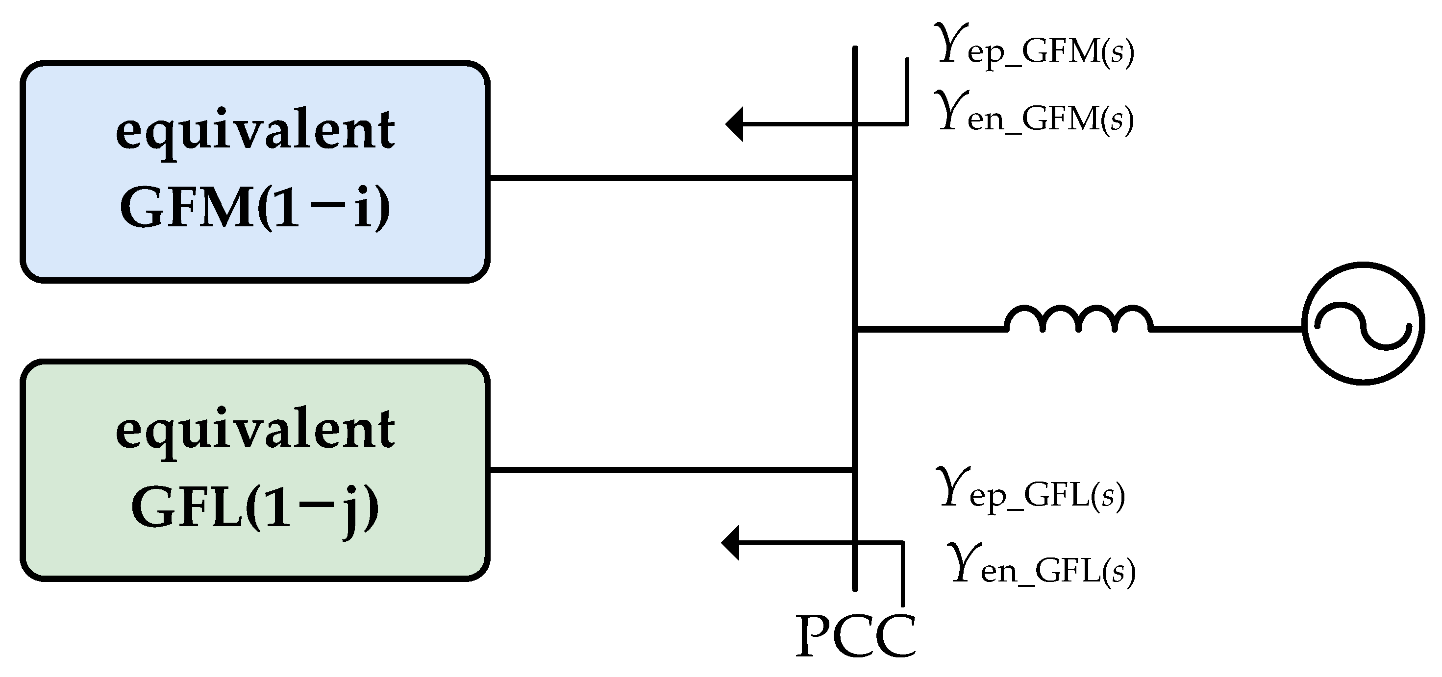
In Equation (15), Y_{ep_GFL}(s), Y_{en_GFL}(s), Y_{ep_GFM}(s), and Y_{en_GFM}(s) represent the admittance matrices for the equivalent grid-following and grid-forming systems. After a reduction in order, the grid-following and grid-forming hybrid renewable energy plant can be simplified to a simple system containing only the equivalent grid-following and grid-forming systems. The topology is shown in Figure 7.

3.4. Model Validation

3.4.1. Inverters Parameter Design

The admittance matrix is measured using the harmonic injection method. A hybrid renewable energy plant consisting of two grid-following inverters and two grid-forming inverters was built in Matlab/Simulink2023a, where harmonic signals of different frequencies are injected at the point of common coupling (PCC), and the resulting harmonic currents are measured. The admittance at each frequency is calculated accordingly. The admittance at each frequency is calculated using the following equation: Y[f] = u[f]/i[f], where u[f] and i[f] are the measured harmonic current and the voltage at the PCC. By comparing the measured admittance values with the calculated results, the accuracy of the model order reduction method is verified.

Next, the parameter design of the grid-following and grid-forming converters is introduced. The grid-following converter design refers to [25], while the main circuit parameters of the grid-forming converter, including the LCL filter, remain the same. For the grid-forming inverter, the most critical aspect lies in the parameter regulation of the active power loop, which can be simplified into a typical second-order system. According to the control block diagram of the active power loop and the power angle equation, the closed-loop transfer function of the active power loop can be obtained as follows:

$$G_{\mathrm{p}}(s)={\displaystyle \frac{1}{J{s}^2+Ds+U_g{E}_0/X_0}}$$

(16)

In the Equation (16), U_g represents the grid voltage, E₀ is the initial voltage of the GFM inverter, and X₀ is the impedance between the initial voltage and the grid voltage. By combining the typical control parameters of a second-order system, the inertia J and damping coefficient D of the grid-forming inverter can be derived.

The parameters for the grid-following and grid-forming inverters are provided in

Table 1. Grid-forming inverter parameters.

Parameter	Value	Parameter	Value
Pn/MW	1	Udc/V	1000
Ug/V	220	L1/mH	0.04125
L2/mH	0.04125	C1/μF	982.44
Ls/mH	0.004125	Lx/mH	0.2475
Dp	202.5079	J/(kg.m2)	10.6583
Dq	10	K	0.1
Lv/mH	0.0016	Rv/Ω	0.05

and

Table 2. Grid-following inverter parameters.

Parameter	Value	Parameter	Value
Pn/MW	1	Udc/V	1000
Ug/V	220	L1/mH	0.04125
L2/mH	0.04125	C1/μF	982.44
Ls/mH	0.004125	Lx/mH	0.2475
Hi	0.00044	KpPLL	253
Hu	0.0034	KiPLL	16,016

.

3.4.2. Admittance Curve Comparison

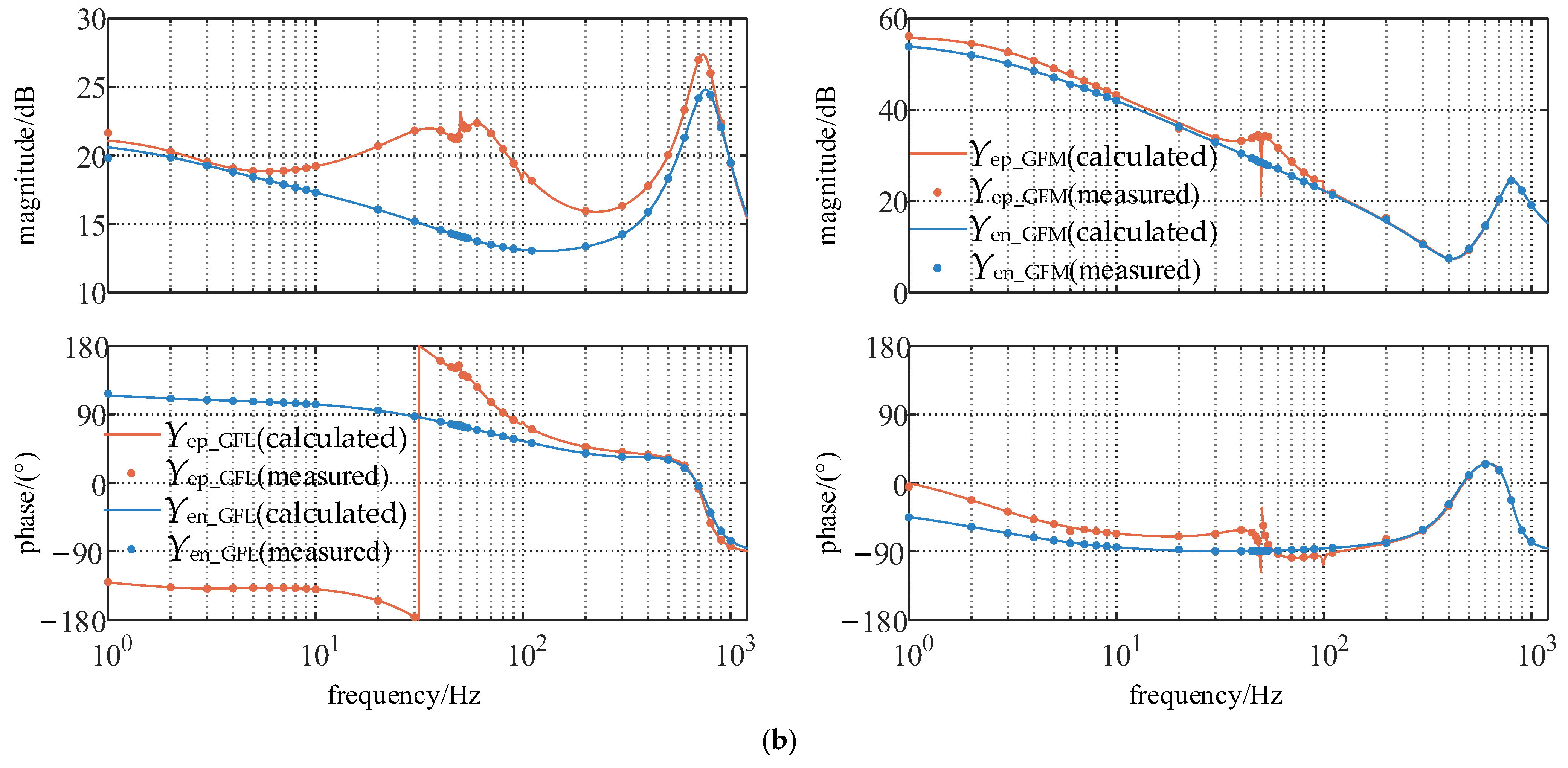
During the modeling process, some studies simplify the calculation by neglecting the coupling effects between the positive and negative sequences [26]. However, as discussed earlier, this approach does not accurately represent the real coupling paths within the system. Ignoring these effects and using the single inverter impedance as the actual impedance of the inverter in the renewable energy plant leads to discrepancies between the calculated and measured values, ultimately impacting the model’s accuracy and reliability. A comparison of the calculated values of the equivalent grid-following and grid-forming admittances, with and without considering coupling effects, demonstrates the importance of frequency decoupling. As shown in Figure 8, the calculated values align perfectly with the simulation results when coupling effects are considered. By contrast, ignoring coupling effects leads to significant discrepancies between the calculated and simulated values. This demonstrates the importance of incorporating coupling effects in impedance modeling.

The simulation validation of the proposed reduced-order modeling method confirms that a grid-following and grid-forming hybrid renewable energy plant can be effectively simplified into a system comprising a grid-following inverter, a grid-forming inverter, and a grid. By following the reduction steps outlined in Figure 4, this simplified model accurately captures the impedance characteristics of the inverters. This reduced-order method categorizes and aggregates different inverters, reducing the admittance matrix of order (2i + 2j) × (2i + 2j) in Equation (4) to a 4th-order equivalent grid-following/grid-forming admittance matrix. Additionally, the order of this equivalent admittance matrix remains constant regardless of the number of inverters. The modeling process incorporates coupling effects to ensure accuracy. By utilizing this reduced-order system, the stability characteristics of the hybrid inverter system can be analyzed, significantly simplifying the stability analysis. The following section will apply this reduced-order modeling approach to assess the stability of grid-following and grid-forming hybrid renewable energy plants.

4. Stability Analysis of Grid-Following and Grid-Forming Hybrid New Energy Power Plants

Grid-following and grid-forming hybrid renewable energy plants exhibit distinct impedance characteristics compared to single-inverter systems, resulting in increased complexity in their stability analysis and necessitating further in-depth investigation. The model order reduction method presented earlier establishes a solid theoretical foundation for the stability studies of such systems. In this section, representative case studies are conducted by integrating the reduced-order model with various stability analysis approaches to systematically examine the underlying mechanisms through which grid-forming inverters enhance the stability of renewable energy plants.

4.1. Stability Analysis Methods

4.1.1. Harmonic Characteristic Analysis Method

As power electronic devices, inverters are susceptible to harmonic distortion. The harmonic characteristic analysis method, based on the impedance approach, enables the examination of an inverter’s amplification or attenuation effects on harmonics, facilitating an analysis of the system’s harmonic behavior across different frequencies.

The harmonic equivalent circuit for a grid-following inverter operating in isolation is shown in Figure 9a, while the harmonic equivalent circuit for a multi-inverter system is illustrated in Figure 9b. An oscillation source, U_p(s), exists on the grid side. When the inverter is disconnected, the harmonics at the grid connection point match those of the grid. However, when the inverter is connected, the harmonics at the connection point change. A lower harmonic content at the connection point is more favorable for the stable operation of the inverter.

To investigate the suppression or amplification of harmonics when grid-side oscillations are transmitted to the point of connection, the transfer function from the grid-side harmonic voltage to the connection point can be calculated. As shown in Figure 9a, the transfer function expression for a system consisting only of a grid-following inverter is as follows:

$$G_{u_{\mathrm{p}}}^{u_{\mathrm{GFLp}}}(s)={\displaystyle \frac{Z_{\mathrm{ep}\_\mathrm{GFL}}(s)}{Z_{\mathrm{g}}(s)+Z_{\mathrm{ep}\_\mathrm{GFL}}(s)}}$$

(17)

$$G_{u_n}^{u_{\mathrm{GFLn}}}(s)={\displaystyle \frac{Z_{\mathrm{en}\_\mathrm{GFL}}(s)}{Z_{\mathrm{g}}(s)+Z_{\mathrm{en}\_\mathrm{GFL}}(s)}}$$

(18)

Based on Figure 9b, the transfer function for the harmonic voltage from the grid to the point of connection in a grid-following and grid-forming hybrid system can be calculated as follows:

$$G_{u_{\mathrm{p}}}^{u_{\mathrm{GFLp}}}(s)={\displaystyle \frac{Z_{\mathrm{ep}\_\mathrm{GFM}}(s)||Z_{\mathrm{ep}\_\mathrm{GFL}}(s)}{Z_{\mathrm{g}}(s)+Z_{\mathrm{ep}\_\mathrm{GFM}}(s)||Z_{\mathrm{ep}\_\mathrm{GFL}}(s)}}$$

(19)

$$G_{u_{\mathrm{n}}}^{u_{\mathrm{GFLn}}}(s)={\displaystyle \frac{Z_{\mathrm{en}\_\mathrm{GFM}}(s)||Z_{\mathrm{en}\_\mathrm{GFL}}(s)}{Z_{\mathrm{g}}(s)+Z_{\mathrm{en}\_\mathrm{GFM}}(s)||Z_{\mathrm{en}\_\mathrm{GFL}}(s)}}$$

(20)

The harmonic characteristic curve of the system is plotted based on Equations (17)–(20). The amplitude–frequency curve illustrates how grid-side disturbances are transmitted to the point of connection across different frequency ranges. An amplitude greater than 1 indicates that the disturbances are amplified at the point of connection, posing a risk of instability, while an amplitude less than 1 indicates that the disturbances are attenuated. If attenuation occurs over a wider frequency range, the control strategy demonstrates stronger disturbance rejection capability, ensuring reliable operation even when grid-side disturbances are present.

4.1.2. Nyquist Stability Criterion of Grid-Following and Grid-Forming Hybrid New Energy Power Plants

Due to the voltage source characteristics of the grid-forming inverter, the three-port network comprising the grid-following inverter, the grid-forming inverter, and the grid can be simplified into a two-port network. In this configuration, the grid-forming inverter operates in parallel with the grid, while the grid-following inverter is connected in series. Figure 10 illustrates the equivalent circuit of the grid-following and grid-forming hybrid renewable energy plant.

The equivalent grid impedance, denoted as Z_sys(s) = Z_GFM(s)||Z_g(s), represents the parallel combination of the grid-forming inverter and the power grid. The equivalent voltage after this parallel connection is represented as U₀(s).

Based on the above analysis, the impedance ratio of the grid-following and grid-forming hybrid renewable energy plant is given by the following:

$$I{R}_{\mathrm{mixp}}(s)={\displaystyle \frac{Z_{\mathrm{sysp}}(s)}{Z_{\mathrm{ep}\_\mathrm{GFL}}(s)}}={\displaystyle \frac{Z_{\mathrm{ep}\_\mathrm{GFM}}(s)||Z_{\mathrm{g}}(s)}{Z_{\mathrm{ep}\_\mathrm{GFL}}(s)}}$$

(21)

$$I{R}_{\mathrm{mixn}}(s)={\displaystyle \frac{Z_{\mathrm{sysn}}(s)}{Z_{\mathrm{en}\_\mathrm{GFL}}(s)}}={\displaystyle \frac{Z_{\mathrm{en}\_\mathrm{GFM}}(s)||Z_{\mathrm{g}}(s)}{Z_{\mathrm{en}\_\mathrm{GFL}}(s)}}$$

(22)

In Equations (21) and (22), Z_{ep_GFL}(s) and Z_{ep_GFM}(s) represent the positive sequence impedances of the equivalent grid-following and grid-forming inverters, while Z_{en_GFL}(s) and Z_{en_GFM}(s) represent their negative sequence impedances, and Z_g(s) is the grid impedance. The stability of the system can be assessed by analyzing whether the Nyquist plot of the open loop transfer functions, as shown in Equations (21) and (22), encircles the point (−1, j0).

4.2. Capacity Ratio Analysis of the Grid-Forming and Grid-Following Hybrid New Energy Power Plants

Grid-following inverters can effectively control harmonic content within a small range under strong grid conditions, resulting in a higher stability margin for the system. However, in weak grid conditions, the stability margin of the inverters decreases, and the risk of harmonic generation increases. To address this, increasing the capacity of the grid-forming inverter in a dual-inverter system can improve the system’s stability [27]. In renewable energy plants, the number of inverters is typically large, and interactions between inverters are likely to occur. This conclusion may require further investigation.

The following section employs the reduced-order modeling method for grid-following and grid-forming inverters to investigate how grid-forming inverters enhance the stability of small grid-following inverters in weak grids. Four scenarios are analyzed, each with a short-circuit ratio of 1.5. To provide a comprehensive assessment of the impact of grid-forming inverters on grid-following systems, Scenario 4 includes two grid-forming inverters with different parameter sets, both of which ensure stable operation in a weak grid with a short-circuit ratio of 1.5.

Table 3. Parameters of four scenarios with different inverters.

	Inverter 1	Inverter 2	Inverter 3	Inverter 4	Total Inverter Capacity
Scenario 1	GFL/1 MW	GFL/1 MW	GFL/0.5 MW	GFL/1 MW	3.5 MW
Scenario 2	GFM/1 MW	GFL/1 MW	GFL/0.5 MW	GFL/1 MW	3.5 MW
Scenario 3	GFM/1 MW	GFM/1 MW	GFL/0.5 MW	GFL/1 MW	3.5 MW
Scenario 4	GFM/1 MW	GFM/1 MW	GFM/0.5 MW	GFL/1 MW	3.5 MW

outlines the inverter configurations for each scenario, while detailed inverter parameters are provided in Appendix A.

To gain a deeper understanding of harmonic suppression in the four scenarios, harmonic characteristic curves were plotted for each case. As shown in Figure 11, when the amplitude of the harmonic characteristic curve exceeds 1, it indicates that disturbances from the power source side are amplified as they propagate to the grid connection point. Conversely, an amplitude below 1 signifies that disturbances are attenuated during transmission. In scenarios where only the grid-following inverters are present, the harmonic characteristic curve exceeds 1 within the 1–176.3 Hz range, indicating that the grid-following inverters amplify harmonics in this frequency band. The harmonic characteristic curves from Scenario 1 to Scenario 3 reveal that, as the grid-forming inverters are introduced, disturbances in the low and medium frequency range are suppressed to varying degrees. Moreover, the suppression effect becomes more pronounced as the number of grid-forming inverters increases. Nevertheless, the harmonic characteristic curve of Scenario 4 shows that, when the grid-forming inverters with different parameters are present in the system, harmonics around 50 Hz and 100 Hz increase significantly, highlighting emerging stability issues among the grid-forming inverters. Both grid-following and grid-forming control loops incorporate feedback mechanisms. Improved harmonic suppression at the point of interconnection results in lower harmonic content in the feedback signals, which in turn enhances system stability. In conclusion, from the perspective of harmonic characteristics, the integration of grid-forming inverters improves the harmonic behavior in the low-to-mid frequency range at the point of common coupling. In a grid-following and grid-forming hybrid renewable energy plant, increasing the number of grid-forming inverters under the same operating conditions significantly reduces harmonic content in these frequency ranges. However, when grid-forming inverters with different operating conditions are added, interactions between the inverters can lead to stability issues around the power frequency.

To comprehensively analyze the impact of inverter configuration on a grid-following and grid-forming hybrid renewable energy plant, impedance curves for the equivalent grid-following and grid-forming systems were plotted for four different scenarios with the same parameters. As shown in Figure 12a, with the increase in grid-forming inverters, the magnitude of the equivalent grid-following impedance gradually increases. In Figure 12b, the impedance of the equivalent grid decreases. The phase margin at the intersection of the equivalent grid-following and grid-forming impedances reflects the stability of the system: PM = 180° − |∠(φ_sys − φ_GFL)|. As seen in Figure 13, from Scenario 1 to Scenario 3, with an increase in the grid-forming inverters, the intersection of the magnitude of the equivalent grid-following impedance and the equivalent grid impedance shifts to the right. The phase angle of the equivalent grid increases, while the phase angle of the equivalent grid-following impedance decreases, causing the phase difference to decrease and the phase margin to gradually increase. As seen in Scenario 4, with the addition of a grid-forming inverter with different parameters from the previous ones, the intersection of the equivalent grid-following and grid-forming impedances shifts to the left near 50 Hz. At this point, the equivalent grid-following impedance lies within the negative damping region, leading to system instability. In conclusion, from the perspective of impedance curves, the addition of grid-forming inverters increases the magnitude of the equivalent grid-following impedance and reduces the magnitude of the equivalent grid impedance. This causes the intersection of the two impedance curves to shift to the right, thereby increasing the phase margin and enhancing system stability. The stability improvement is more significant when grid-forming inverters with the same operating conditions are added. However, when grid-forming inverters with different operating conditions are introduced, the impedance intersection shifts earlier, leading to a risk of system instability.

To analyze the stability of the four scenarios, the solid and dashed lines in Figure 14 represent the positive sequence and negative sequence Nyquist curves. In scenarios one and four, the Nyquist curves pass through (−1, j0), indicating system stability. By contrast, the Nyquist curves in scenarios two and three do not pass through (−1, j0), indicating system instability. This result aligns with the previous stability analysis, which suggests that adding grid-forming inverters with the same operating conditions to a grid-following system improves system stability, while introducing different inverters poses a risk of instability.

To conclude, the addition of grid-forming inverters improves the harmonic content at the grid connection point, reduces the control complexity of both the grid-following and grid-forming inverters, and enhances the system’s disturbance rejection capability. From the perspective of system impedance, the inclusion of the grid-forming inverters increases the impedance of the equivalent grid-following inverter and decreases the impedance of the equivalent power grid, shifting the impedance intersection to the right, while increasing the stability margin. However, when multiple grid-forming inverters with different operating conditions are present in the system, their interactions may introduce new stability issues.

5. Simulation Verification

To validate the conclusions in Section 4, simulation models for the four scenarios were constructed under the condition of SCR = 1.5. The inverter current waveforms are shown in Figure 15a. As depicted, the current waveforms in Scenario 1 and Scenario 4 exhibit significant oscillations, whereas those in Scenarios 2 and 3 remain stable. This corresponds with the stability analysis presented in Section 4.2. Figure 15b analyzes the harmonic content of the current. In Scenario 1, the dominant harmonics are 13.8 Hz and 86.2 Hz, while in Scenario 4, the dominant harmonics are 49 Hz and 51 Hz, which aligns with the harmonic characteristic analysis from Section 4.2.

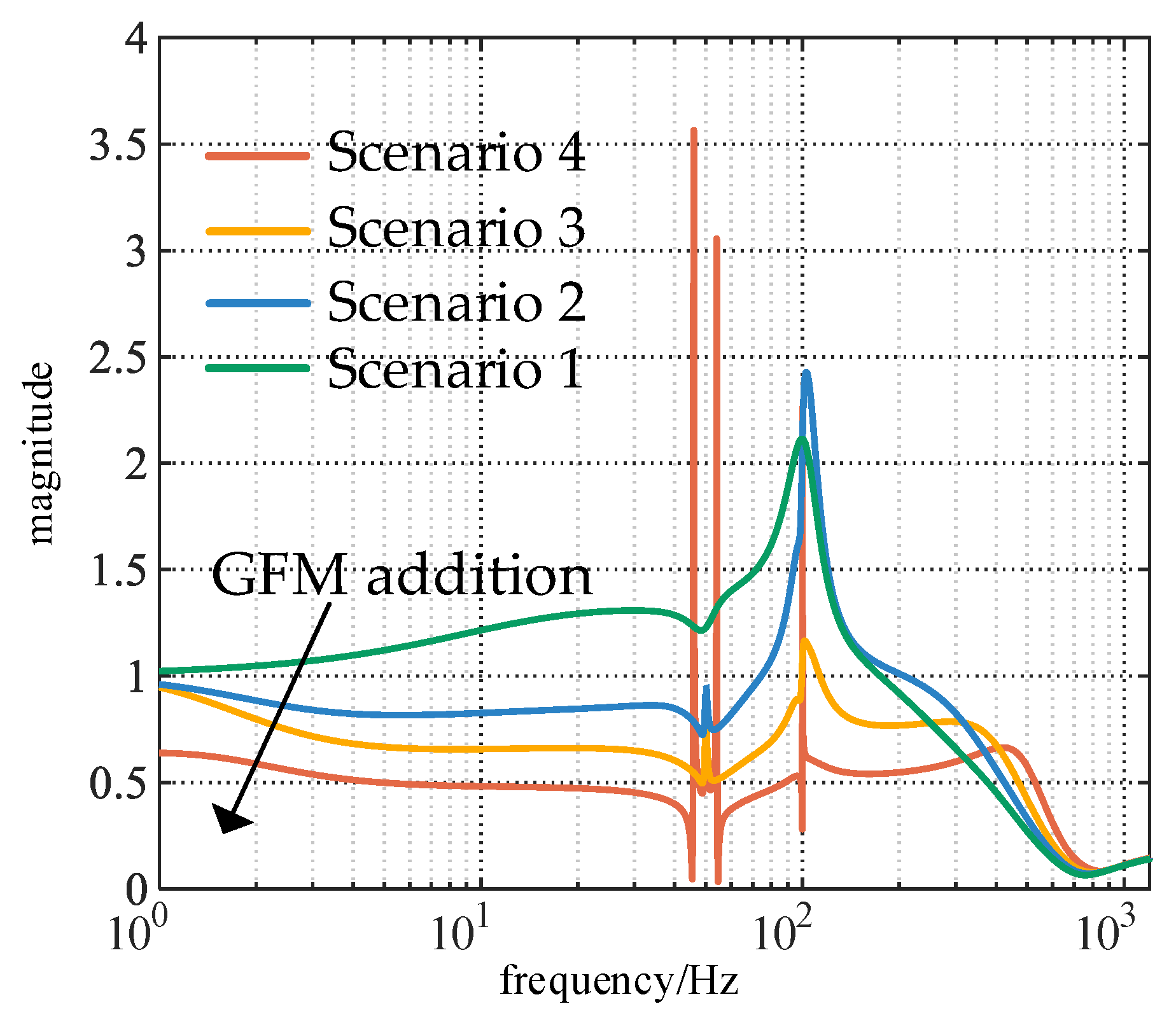
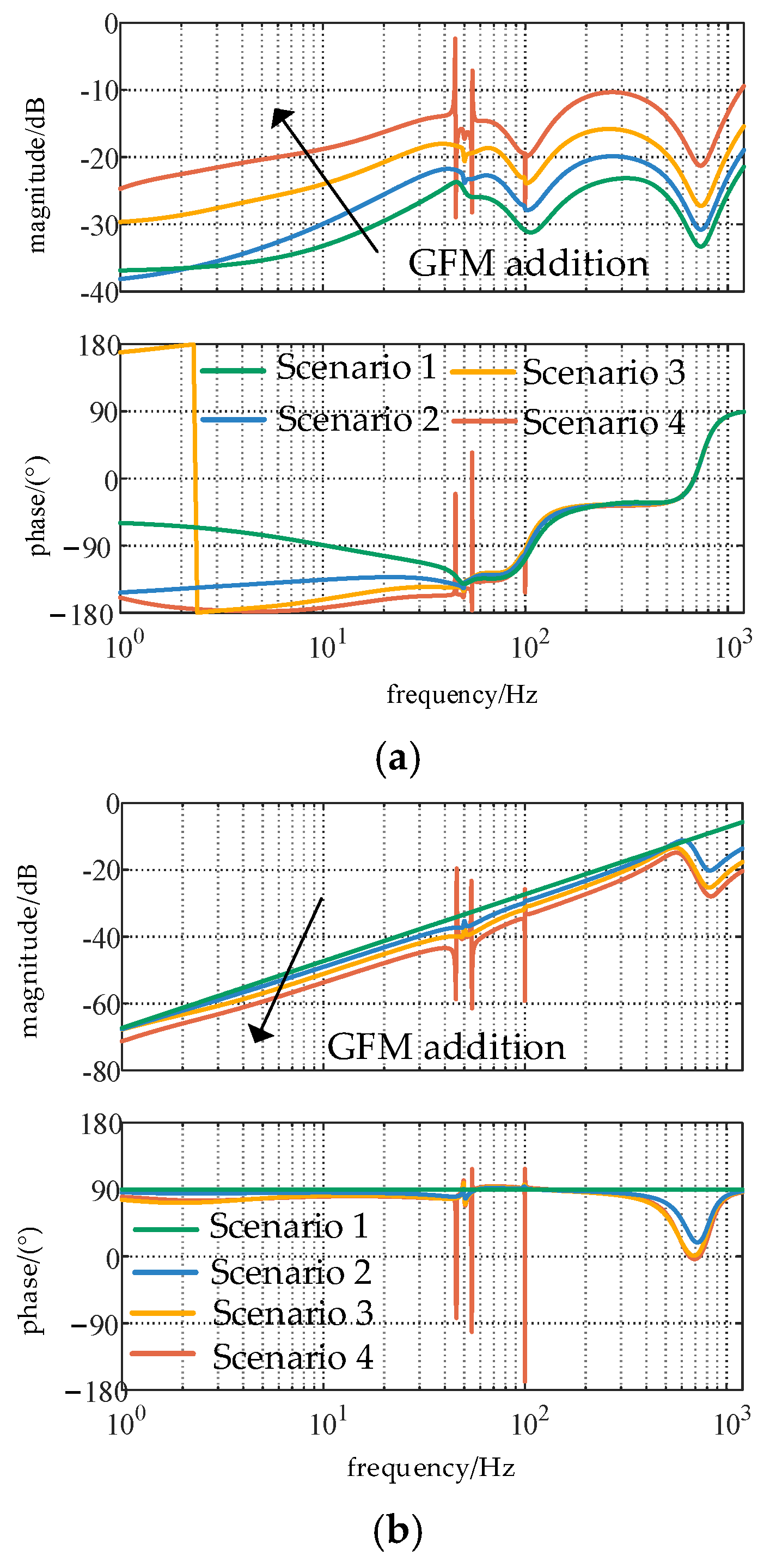
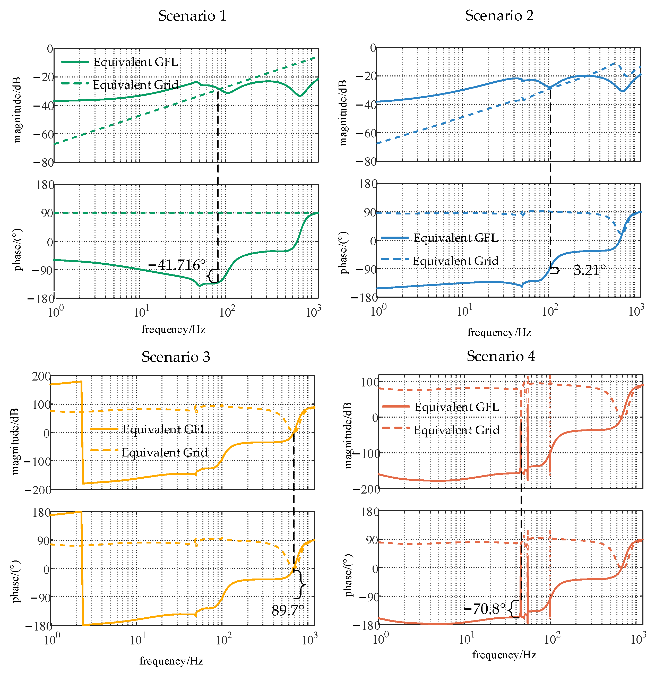
Overall, the consistency between simulation experiments and theoretical analysis demonstrates that the impedance matrix calculated via the reduced-order modeling method effectively reflects the impedance characteristics of the grid-following and grid-forming hybrid renewable energy plants, thereby enabling accurate stability assessments. Simulation results across various scenarios further indicate that incorporating grid-forming inverters into renewable energy plants with multiple grid-following inverters can suppress harmonics in the low and medium frequency ranges at the connection point, and reduce the harmonic content in the feedback control loops of both inverter types. Adjusting the impedance magnitudes of the equivalent grid-following inverter and the equivalent grid indirectly enhances the system’s phase margin, thereby improving its overall stability. However, if a grid-following and grid-forming hybrid renewable energy plant includes multiple grid-forming inverters under different operating conditions, interactions among these units may introduce new stability challenges.

6. Conclusions

This paper presents a reduced-order modeling approach for grid-following and grid-forming hybrid renewable energy plants. By employing harmonic characteristic analysis and the Nyquist stability criterion, this study examines how grid-forming inverters enhance the stability of grid-following inverters in weak grid conditions. Additionally, this study explores the capacity ratio between grid-following and grid-forming inverters in the plant. The main contributions and conclusions are summarized as follows:

(1) For grid-following and grid-forming hybrid renewable energy plants, the proposed reduced-order modeling method employs the aggregation of inverters with similar control strategies and the decoupling of positive and negative frequency among different components. This approach simplifies the complex renewable energy plant into a straightforward system comprising an equivalent grid-following system, an equivalent grid-forming system, and the power grid, thereby combining simplicity and generality with accuracy.

(2) The incorporation of grid-forming inverters markedly reduces the harmonic content in the low-to-medium frequency range at the grid connection point. In addition, by increasing the magnitude of the equivalent grid-following impedance while decreasing that of the equivalent grid impedance, the phase margin of the renewable energy plant is indirectly enhanced, thereby improving the stability of grid-following inverters under weak grid conditions. However, when multiple grid-forming inverters are present, caution must be exercised, since interactions among them may give rise to new stability challenges.

In addition, one small limitation of this paper is that none of the content has been experimentally validated in the laboratory. We will address this limitation in future work.