Research on the Construction Method of Inter-Provincial Spot Trading Network Model Considering Power Grid Congestion

Abstract

This study proposes a full-cost electricity pricing model (M3) based on power flow tracing, addressing limitations in traditional nodal pricing and postage stamp methods. M3 dynamically allocates fixed transmission costs based on actual grid utilization, improving fairness, price signal accuracy, and congestion management. The model achieves fast convergence within 20 iterations across tested networks. Sensitivity analysis confirms that fuel costs and load variations significantly impact pricing, making M3 more adaptive and responsive. A regression-based forecasting model further enhances price predictability. The dual IEEE 118-bus case study validates M3’s feasibility in inter-provincial electricity markets, demonstrating its effectiveness for real-time pricing and investment planning.

1. Introduction

With the deepening of electricity market reform, the efficiency and fairness of power grid resource allocation have become central issues in electricity market research. The current nodal pricing system typically considers only the marginal cost of generation while neglecting fixed transmission costs, leading to incomplete price signals that fail to reflect the actual utilization of grid resources by the load [1]. Additionally, traditional transmission cost allocation mechanisms lack scientific rigor and fairness, suppressing the potential for demand-side response and potentially inducing inefficient expansion of the transmission network, thereby reducing overall grid efficiency.

In recent years, scholars have conducted extensive research on nodal pricing systems and transmission cost allocation, achieving significant progress. Regarding nodal pricing, the marginal cost-based nodal pricing system has been widely applied, but it generally assumes an uncongested transmission network, overlooking the impact of fixed transmission costs on nodal prices [2,3,4]. Some studies have proposed improved models that incorporate fixed transmission costs into electricity pricing [5,6]; however, they lack a mechanism to distinguish between effective transmission costs, which reflect actual grid utilization, and ineffective transmission costs, which do not accurately represent resource usage, leading to inaccurate price signals. [7]. A major limitation of these models is that they cannot address the true complexities of large-scale grids where power flow tracing plays a critical role in ensuring accurate cost allocation. This paper proposes an innovative solution by introducing power flow tracing technology that dynamically allocates transmission costs based on actual power flows, improving both fairness and efficiency in transmission cost allocation.

The proposed full-cost electricity pricing model integrates generation marginal costs with effective transmission costs, offering a more accurate and dynamic allocation method compared with traditional approaches. The introduction of power flow tracing technology represents a key advancement by distinguishing between effective and ineffective transmission costs, which current models fail to do. Additionally, this model addresses grid congestion more accurately by incorporating its impact on pricing, a significant improvement over existing models.

Regarding transmission cost allocation, power flow tracing technology is regarded as an important tool for reasonably allocating transmission costs. It traces the distribution of power flows between generation and load nodes, clarifying each node’s contribution to line flows. Although postage stamp methods are widely used to allocate fixed transmission costs, some markets adopt coincident peak methods, which allocate transmission costs based on actual grid utilization. However, even with these methods, the price signals still fail to fully incentivize load-side adjustments in electricity consumption behavior because they do not always reflect the dynamic nature of power grid utilization, which limits the effectiveness of demand response [8,9,10,11]. The introduction of power flow tracing technology in this study is a significant innovation, offering a more dynamic, accurate, and fair approach to transmission cost allocation, ensuring that each node pays its fair share of the grid costs.

Demand response and grid congestion have also become major research areas, with demand response considered a crucial tool to improve grid resource utilization efficiency [12]. However, under the current electricity pricing mechanism, price signals fail to incentivize load-side adjustments, especially when coincident peak methods are used to allocate transmission costs, as these methods do not fully reflect the dynamic utilization of transmission resources. Moreover, grid congestion is often simplified in many studies, without fully reflecting its impact in pricing models. This paper proposes an innovative solution to address grid congestion more accurately and integrates it into the pricing model.

To address these issues, this paper proposes a full-cost electricity pricing model based on power flow tracing technology and designs a spot market trading network model suitable for inter-provincial AC grid congestion. The main contributions of this study include the following:

• Dynamic full-cost electricity pricing based on power flow tracing. This study introduces a full-cost electricity pricing model that dynamically integrates marginal generation costs and effective transmission costs using power flow tracing. Unlike traditional nodal pricing, which ignores fixed transmission costs, M3 ensures cost allocation proportional to actual grid utilization, enhancing fairness and pricing accuracy in electricity markets.
• Computationally efficient and adaptive pricing mechanism. The proposed model achieves fast convergence within 20 iterations across all tested networks, demonstrating its computational feasibility for real-time pricing applications. Sensitivity analysis confirms that fuel cost fluctuations and load variations significantly impact electricity pricing, making M3 a more adaptive and responsive pricing method compared with existing approaches.
• Regression-based price forecasting for market predictability. A regression-based forecasting model is incorporated to quantify the relationship between key economic factors (fuel costs, demand response, transmission constraints) and nodal prices. The model achieves a high R² score (above 0.88) across test cases, validating its effectiveness in predicting electricity price trends. This enhances M3’s applicability in real-time market operations, investment planning, and demand-side response strategies.

2. Materials and Methods

2.1. Fundamental Concept of Full-Cost Electricity Pricing

The current nodal pricing system does not incorporate the recovery of fixed transmission costs resulting from investments in transmission. Under the assumptions of a lossless DC power flow and an uncongested network, nodal prices remain uniform across different locations, failing to accurately reflect the impact of full generation and transmission costs on the spatial and temporal distribution of load. Additionally, traditional transmission cost allocation mechanisms do not distinguish between effective and ineffective transmission costs, making it difficult for the allocation results to truly reflect the utilization of grid resources by the load. This inefficiency in cost allocation negatively affects grid investment efficiency and contradicts the principles of optimal resource allocation [13,14].

To address these issues, this paper introduces the concept of full-cost electricity pricing, which integrates generation marginal costs with effective transmission costs [15,16,17,18]. By employing power flow tracing techniques, the proposed pricing model reasonably allocates fixed transmission costs, ensuring that electricity prices dynamically reflect the extent to which loads utilize grid resources while adhering to the principle of “costs borne by beneficiaries”. Effective transmission costs are further classified into regular operational costs, N-1 security operational costs, future load growth costs, and ineffective transmission costs, ensuring that pricing signals remain fair and accurate while truly reflecting the actual cost of grid resource utilization by loads.

This paper defines the permitted cost recovery rate of transmission line $j$ at time $t$ as follows:

$$r_{j,t}={\displaystyle \frac{\left|f_{j,t}^{OC}\right|+\left({\tilde{f}}_{j,t}^c-\left|f_{j,t}^{OC}\right|\right)}{F_{j,max}}}\hspace{1em}={\displaystyle \frac{{\tilde{f}}_{j,t}^c}{F_{j,max}}}$$

(1)

where

$${\tilde{f}}_{j,t}^c=\underset{c^{,}\in \left\{0\right\}\cup C}{max}\left|f_{j,t}^{c^{,}}\right|$$

(2)

In these equations:

$F_{j,max}$ is the capacity of transmission line $j$.

$f_{j,t}^{OC}$ represents the base case power flow of transmission line $j$.

${\tilde{f}}_{j,t}^c$ is the maximum absolute value of the power flow on transmission line $j$ across the base case and all N-1 contingency scenarios.

The effective fixed transmission cost of transmission line $j$ at time $t$ is then calculated as:

$$C_j^{VT}=r_{j,t}{C}_j^T$$

(3)

where $C_j^T$ represents the total transmission investment cost of line $j$.

2.2. Derivation of Full-Cost Electricity Pricing Based on Power Flow Tracing Method

The power flow tracing method is a technique used to allocate the utilization of grid resources by generation and load nodes by analyzing power flow paths within the grid. In electricity markets, power flow tracing is widely applied to distribute transmission costs and identify the contribution relationships among grid resources. The fundamental assumption of this method is that the power injected at a node is fully mixed, and the power flowing out of a node is proportionally shared among the downstream branches. This method ensures both transparency in grid resource utilization and fairness in cost allocation.

Assuming that the power injected into and withdrawn from node $k$ e satisfies the following balance equation:

$$P_k=\sum _{\forall j\in \left(k,:\right)}\left|F_j\right|+P_k^L$$

(4)

where $P_k$ is the total injected power at node $k$; $P_k^L$ is the load power at node $k$; $\left(k,:\right)$ denotes the set of lines where node $k$ is the upstream node; $F_j$ is the power flow on transmission line $j$.

Rearranging the equation:

$$P_k-{\displaystyle \frac{{\sum }_{\forall j\in \left(k,:\right)}\left|F_j\right|}{P_k}}{P}_k=P_k^L$$

(5)

Expressed in matrix–vector form, the backward flow tracing equation is given as:

$$A_{d}P=P_L$$

(6)

where $A_d$ is the backward flow tracing matrix, which represents the power flow distribution in the reverse direction. The elements of $A_d$ are defined as:

$$[A_d{]}_{mn}=\left\{\begin{array}{cc}1\hfill & if m=n\\ -{\displaystyle \frac{\left|F_{\left(m,n\right)}\right|}{P_n}}& if n is a downstream node of m\\ 0\hfill & otherwise\end{array}\right.$$

(7)

If $A_d$ is invertible, the node injection power vector can be obtained as:

$$P=A_d^{-1}{P}_L$$

where the $m$-th element of the vector is:

$$P_m=\sum _{k=1}^{N_l}[A_d^{-1}{]}_{mk}{P}_{Lk}$$

(8)

For power flow allocation on line $\left(m,n\right)$, the contribution of load node $k$ to the power flow on this line can be computed using the elements of the inverse backward flow tracing matrix $A_d^{-1}$:

$$F_{\left(m,n\right)}={\displaystyle \frac{F_{\left(m,n\right)}}{P_m}}{\displaystyle \sum _{k=1}^{N_l}{[A_d^{-1}]}_{mk}{P}_k^L}\hspace{1em}$$

(9)

Furthermore, the total contribution of node $k$ to the power flows across all transmission lines in the grid can be obtained by summing over all transmission lines. Combining this with the effective transmission cost $C_j^{VT}$, the total transmission cost borne by node $k$ can be expressed as:

$$C_k^{TC}=\sum _{\forall F_j=F_{\left(m,n\right)}}\left({\displaystyle \frac{F_j}{P_m}}[A_d^{-1}{]}_{mk}{P}_k^L{\displaystyle \frac{r_{k.t}{C}_j^T}{F_j}}\right)$$

(10)

where

$C_k^{UT}$ represents the total transmission cost borne by node $k$;

$C_j^T$ is the total investment cost of transmission line $j$;

$r_{k.t}$ is the permitted fixed transmission cost recovery rate of the line.

The unit transmission cost at node $k$ is then calculated as:

$$\begin{array}{cc}\hfill C_k^{UT}& ={\displaystyle \frac{C_k^{TC}}{P_k^L}}\hfill \\ & ={\displaystyle \sum _{\forall F_j=F_{\left(m,n\right)}}\left(\frac{r_{k.t}{C}_j^T}{P_i}{\left[A_d^{-1}\right]}_{ik}\right)}\hfill \end{array}$$

(11)

This unit transmission cost explicitly reflects the utilization of transmission network resources by each load node.

Finally, the full-cost electricity price at node $k$ is obtained by linearly combining generation costs and transmission costs:

$$\begin{array}{cc}\hfill {\pi }_{k,t}& ={\rho }_{k,t}+C_k^{UT}\hfill \\ & ={\rho }_{k,t}+{\displaystyle \sum _{\forall j(:,i)}\left(\frac{F_j}{P_i}{\left[A_d^{-1}\right]}_{ik}\frac{C_j^T}{F_j}{r}_{k.t}\right)}\hfill \\ & ={\rho }_{k,t}+{\displaystyle \sum _{\forall j(:,i)}\left(\frac{C_j^T}{P_i}{\left[A_d^{-1}\right]}_{ik}{r}_{k,t}\right)}\hfill \end{array}$$

(12)

where

${\rho }_{\mathrm{k}}$ represents the marginal generation cost at node $k$;

$C_k^{UT}$ is the unit transmission cost component.

In this study, voltage stability and transformer overload constraints are directly modeled and incorporated into the power flow tracing calculations to ensure that the power flow remains within operational limits, reflecting real-world grid security conditions.

We model voltage stability by setting voltage limits at each node. These limits ensure that the voltage at each node remains within an acceptable range, typically between 0.95 p.u. (per unit) and 1.05 p.u. (per unit). This ensures that the voltage levels do not exceed operational limits, which could lead to instability or equipment damage. The voltage at node $k$ is constrained as follows:

$$V_k^{min}\le V_k\le V_k^{max}$$

(13)

where $V_k^{min}$ and $V_k^{max}$ represent the lower and upper voltage limits at node $k$, respectively.

For transformer overload constraints, we model the power flow through each transformer to ensure that it does not exceed its rated capacity. If the power flow through a transformer exceeds its capacity, the system is considered overloaded. The transformer overload constraint for transformer $t$ is given by:

$$\left|F_t\right|\le F_{t,max}$$

(14)

where $\left|F_t\right|$ represents the power flow on transformer t, and $F_{t,max}$ is the rated capacity of transformer $t$.

These constraints are incorporated into the economic dispatch problem and are enforced during the iterative calculation process to ensure that the power flow adheres to the security limits of the system. By considering these constraints, we ensure that the model operates within realistic security boundaries, reflecting the actual operational limits of the grid.

2.3. Algorithm Convergence and Computational Feasibility

To ensure the stability and reliability of the model, we introduce a convergence analysis of the iterative calculation method. The iterative method used in this study is based on a sequential update of nodal prices using a linear programming (LP) solver. At each iteration, the nodal marginal costs and transmission costs are updated based on the latest economic dispatch results. The algorithm continues until the difference in the full-cost electricity price vector between two consecutive iterations falls below a predefined convergence threshold (ε).

In our case, we have verified that the iterative method converges within a limited number of iterations (typically fewer than 20) for the IEEE 30-bus and IEEE 118-bus systems. Future work will investigate the robustness of this approach for larger-scale systems, including its performance under various grid configurations and its applicability to real-world inter-provincial grid systems.

The iterative calculation primarily employs a damped update strategy to prevent price oscillations during iterations, ensuring greater algorithm stability. The convergence analysis also discusses the computational feasibility of the proposed model. The model’s algorithm complexity is evaluated in terms of the number of iterations required for convergence and its performance in larger more complex grids, such as the dual IEEE 118-bus system used in this study to simulate inter-provincial grid operation. The detailed mathematical formulation of the iterative calculation can be found in Appendix A.2 and Appendix A.3.

The full-cost electricity pricing model allocates total grid costs based on power flow tracing, reflecting differences in grid utilization due to the spatial distribution of loads. This approach ensures that nodes bear differentiated generation and transmission costs, leading to a more equitable and efficient electricity pricing system [19].

The calculation process for full-cost electricity pricing is illustrated in the following flowchart as shown in Figure 1:

3. Case Study

3.1. Case Study on Power Flow Tracing Model

To validate the effectiveness of the proposed full-cost electricity pricing model, this section presents a case study comparing three different pricing schemes. The full-cost electricity price under each scheme is analyzed as follows:

Scheme M1: nodal marginal price without considering the power flow tracing method.

Scheme M2: full-cost electricity price without considering the effectiveness of fixed transmission costs.

Scheme M3: full-cost electricity price incorporating the power flow tracing method.

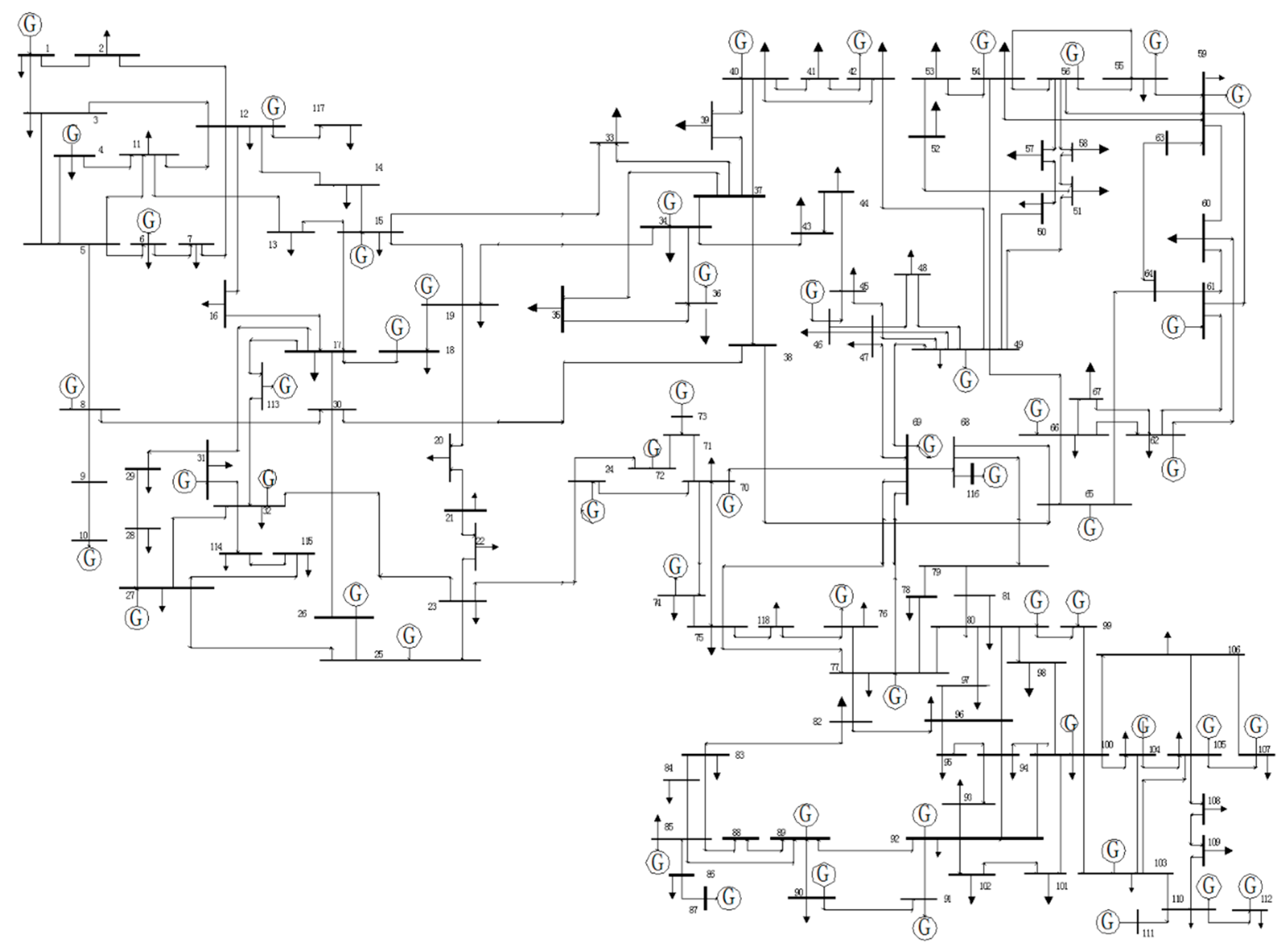
The IEEE 118-bus system (As shown in Figure 2) is selected as the test system to illustrate the significance of the proposed full-cost pricing model based on power flow tracing. The IEEE 118-bus system consists of 54 generating units and 186 transmission lines, providing a complex network structure and boundary conditions suitable for evaluating the model’s performance.

The dataset used for this study, including electricity prices, transmission line parameters, and generator characteristics, is obtained from the SCADA system database provided by the state grid dispatching department. For confidentiality, certain generator data have been anonymized while preserving statistical integrity.

A comparative analysis of nodal electricity prices under the three pricing schemes is conducted.

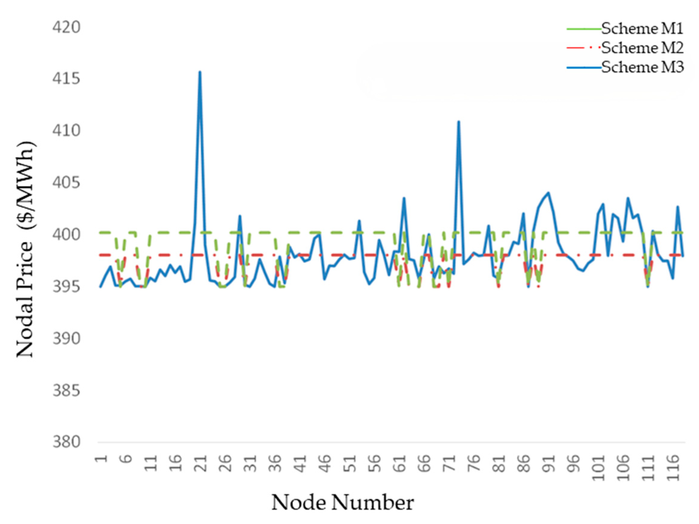
Figure 3 presents a comparison of full-cost electricity prices in the IEEE 118-bus system under three different schemes. It can be observed that the nodal prices in Scheme M1 remain uniform across all nodes, while in Schemes M2 and M3, the nodal prices at terminal nodes exhibit differentiation. The nodal prices at locations far from generation centers (e.g., nodes 25, 44, 73, 114) are significantly higher than those near load centers (e.g., nodes 9, 34, 65, 87). Moreover, at nodes far from generation centers, the full-cost electricity prices in Scheme M3 are significantly lower than those in Scheme M2. Overall, the full-cost electricity prices in Scheme M2 are higher than those in Scheme M3.

The case study results indicate that Scheme M1, based on traditional nodal marginal pricing, does not account for fixed transmission costs. Under the DC power flow model, if no congestion occurs, the marginal price remains uniform across all nodes, failing to capture the variations in electricity consumption across different locations.

Scheme M2 incorporates the full cost of fixed transmission into nodal pricing. The analysis reveals that remote load nodes, due to their greater distance from generation centers, bear the cost of the entire transmission corridor, resulting in significantly higher transmission costs. This full-cost electricity pricing model partially reflects the cost heterogeneity of electricity consumption across nodes by distributing fixed transmission costs accordingly. However, as it does not differentiate between effective and ineffective transmission costs, it fails to account for the actual utilization of each transmission line in the price signals. Consequently, the pricing signals generated are not entirely accurate, leading to an overall higher electricity cost at terminal nodes. This, in turn, may over-incentivize transmission investments, thereby reducing overall investment efficiency.

In contrast, Scheme M3, as proposed in this study, integrates nodal marginal generation costs with effective transmission costs to establish a full-cost electricity pricing framework. The results demonstrate that this pricing approach accurately reflects the extent to which each terminal node utilizes grid resources, thereby capturing the true cost of electricity consumption across different locations and conveying more precise price signals. Under this framework, full-cost electricity pricing aligns with the actual utilization of transmission infrastructure, ensuring that overinvestment is not factored into cost allocation. This effectively mitigates excessive investment incentives for transmission infrastructure, enhances investment efficiency, and ultimately achieves optimal resource allocation. The case study findings validate the superiority of the proposed full-cost electricity pricing model.

To better illustrate the differences among the three pricing strategies,

Table 1. Total cost comparison in IEEE 30-bus system network.

Scheme	Total Generation Cost ($)	Total Transmission Cost ($)	Total Consumption Cost ($)
M1	87,799.84	8363.00	96,162.84
M2	86,888.47	4157.00	91,045.46
M3	86,180.01	3960.53	90,140.54

summarizes their key characteristics.

3.2. Security-Constrained Power Spot Market Based on Power Flow Tracing Method

Under the concept of full-cost electricity pricing based on power flow tracing, a spot market clearing model is formulated.

3.2.1. Objective Function

The objective function of security-constrained economic dispatch based on full-cost electricity pricing is to minimize total generation costs, as expressed in Equation (15):

$$\mathit{min}{\sum }_{k=1}^n{C}_k^G{P}_k^G$$

(15)

where $C_k^G$ represents the unit generation cost of the generator at node $k$; $P_k^G$ is the generation output at node $k$; $n$ is the total number of nodes.

3.2.2. Constraints

(1)

Generation-load balance constraint:

$$\sum _{k=1}^n{P}_k^G=\sum _{k=1}^n{P}_k^L,\forall k$$

(16)

where $P_k^L$ is the load demand at node $k$.

(2)

Generator output limits:

$$P_{k,min}^G\le P_k^G\le P_{k,max}^G$$

(17)

where $P_{k,max}^G$ and $P_{k,min}^G$ denote the maximum and minimum output limits of generator $k$, respectively.

(3)

Transmission line flow limits:

$$-F_{j,max}{\le F_j\le F}_{j,max}$$

(18)

where $F_{j,max}$ represents the active power transmission capacity of line $j$.

(4)

Power flow and generation output transfer distribution factor constraint:

$$F_j=\sum _{k=1}^n{G}_{j-k}\left(P_k^G-P_k^L\right),\forall j$$

(19)

where $G_{j-k}$ represents the generation transfer distribution factor, indicating the sensitivity of power flow on transmission line $j$ to the generation output at generator $k$.

(5)

Full-cost electricity pricing constraint:

Based on the derivation of full-cost electricity pricing, the corresponding constraint is expressed as:

$$\begin{array}{c}{\pi }_{k,t}={\rho }_{k,t}+{\displaystyle \sum _{\forall j(:,i)}\left(\frac{F_j}{P_i}{\left[A_d^{-1}\right]}_{ik}\frac{C_j^T}{F_j}{r}_{k.t}\right)}\\ ={\rho }_{k,t}+{\displaystyle \sum _{\forall j(:,i)}\left(\frac{C_j^T}{P_i}{\left[A_d^{-1}\right]}_{ik}{r}_{k,t}\right)}\end{array}$$

(20)

(6)

Demand response function:

$$P_k^L=f\left({\pi }_{k,t}\right)$$

(21)

where $f\left({\pi }_{k,t}\right)$ denotes the demand response function at load node $k$, which can be formulated in various forms depending on specific modeling requirements. For the purpose of analytical simplification, this study adopts a linear demand response function, where the adjustment range of demand response is constrained by the upper and lower bounds of the load decision variables [20].

The incorporation of power flow tracing techniques introduces matrix inversion operations and other complex nonlinear expressions, leading to a highly nonlinear model that presents significant computational challenges for direct solution.

To address this issue, an iterative computation approach is proposed in this section. The steps for solving the model are as follows [21]:

(1)

Set the initial load values and system network boundary conditions.

(2)

Use a linear programming (LP) solver to compute the economic dispatch.

(3)

Calculate the marginal generation cost and transmission cost based on the economic dispatch results to obtain the full-cost nodal electricity price. If the convergence condition is met (i.e., the two-norm difference of the full-cost electricity price vector between two consecutive iterations is below the threshold), proceed to Step 6; otherwise, go to Step 4.

(4)

The nodal load responds to the full-cost electricity price.

(5)

Update the initial load values and return to Step 2.

(6)

Terminate the computation.

The solution process is shown in Figure 4.

3.3. Case Study on Security-Constrained Economic Dispatch in the Power Spot Market

This section evaluates the effectiveness of the proposed security-constrained economic dispatch model based on full-cost electricity pricing through case studies on the IEEE 30-bus system and IEEE 118-bus system.

Since the iterative solution approach is adopted, the demand-side response function can take different functional forms. For simplification, this study assumes a linear demand response function, as given in Equations (3)–(8):

$$P_{Lk}=-a_k{C}_{Uk}+b_k$$

(22)

In the formula, $a_k$ is set to 0.007, and $b_k$ is taken as the initial load value from the IEEE standard system.

This section compares three node pricing and demand response schemes as follows:

Scheme M1: Nodal prices exclude fixed transmission costs, with demand response based on marginal prices. Fixed transmission costs are not differentiated and are allocated to end-users using the postage stamp method after response.

Scheme M2: Nodal prices include fixed transmission costs, with demand response based on full-cost prices. Effective and ineffective transmission costs are differentiated and allocated using the postage stamp method.

Scheme M3 (proposed): An economic dispatch model incorporating both marginal generation and fixed transmission costs. Demand response is based on full-cost prices, and transmission costs are differentiated and allocated using the power flow tracing method.

The model’s effectiveness is validated through tests on the IEEE 30-bus system and a provincial grid dataset, solved using the CPLEX solver (GAP = 0). Appendix A,

Table A1. Generator parameters.

Unit ID	Capacity (MW)	Node Location	Operating Cost ($/MWh)
1	100	1	380
2	100	2	400
3	100	5	370
4	100	8	390
5	140	11	350
6	100	13	360

and

Table A2. Transmission line parameters.

Line ID	Start–End Node IDs	Transmission Capacity (MW)	Reactance (p.u.)	Investment Cost ($/M)
1	1–2	10	0.575	61.5
2	1–3	10	0.165	169.2
3	2–4	15	0.173	177.7
4	3–4	20	0.037	41.9
5	2–5	5	0.198	202.3
6	2–6	10	0.176	180.3
7	4–6	15	0.041	45.4
8	5–7	10	0.116	120
9	6–7	30	0.082	86
10	6–8	30	0.042	46
11	6–9	80	0.205	212
12	6–10	15	0.556	560
13	9–11	150	0.208	212
14	9–10	80	0.110	114
15	4–12	50	0.256	260
16	12–13	150	0.140	144
17	12–14	20	0.256	259.9
18	12–15	30	0.130	134.4
19	12–16	20	0.198	202.7
20	14–15	10	0.199	203.7
21	16–17	20	0.192	196.3
22	15–18	20	0.219	222.5
23	18–19	10	0.129	133.2
24	19–20	5	0.068	72
25	10–20	10	0.209	213
26	10–17	5	0.085	88.5
27	10–21	30	0.075	78.9
28	10–22	20	0.150	153.9
29	21–22	5	0.023	27.6
30	15–23	20	0.202	206
31	22–24	20	0.179	183
32	23–24	20	0.270	274
33	24–25	20	0.330	333.2
34	25–26	10	0.380	384
35	25–27	10	0.209	212.7
36	27–28	20	0.396	400
37	27–29	10	0.415	419.3
38	27–30	10	0.603	606.7
39	29–30	5	0.453	457.3
40	8–28	5	0.200	204
41	6–28	20	0.600	63.9

list the basic parameters for generators and transmission lines in the IEEE 30-bus system, respectively.

Table 1 compares the generation, transmission, and consumption costs under the three schemes as follows:

Generation cost: Scheme M1, based on nodal marginal pricing without including fixed transmission costs, distorts price signals and limits user response. As a result, generation cost savings are minimal, leading to higher generation costs compared with Schemes M2 and M3.

Transmission cost: Scheme M1 fails to differentiate between the effectiveness of fixed transmission costs, leading to significantly higher transmission costs than in Schemes M2 and M3. Scheme M3, using power flow tracing, more accurately allocates transmission costs, optimizing flow distribution and further reducing total transmission costs.

Consumption cost: Scheme M3 results in the lowest total consumption cost, demonstrating that the full-cost pricing economic dispatch model effectively incentivizes user response, thereby reducing consumption costs.

As shown in

Table 2. Total system load comparison.

Scheme	Total Load (MW)
M1	244.38
M2	241.85
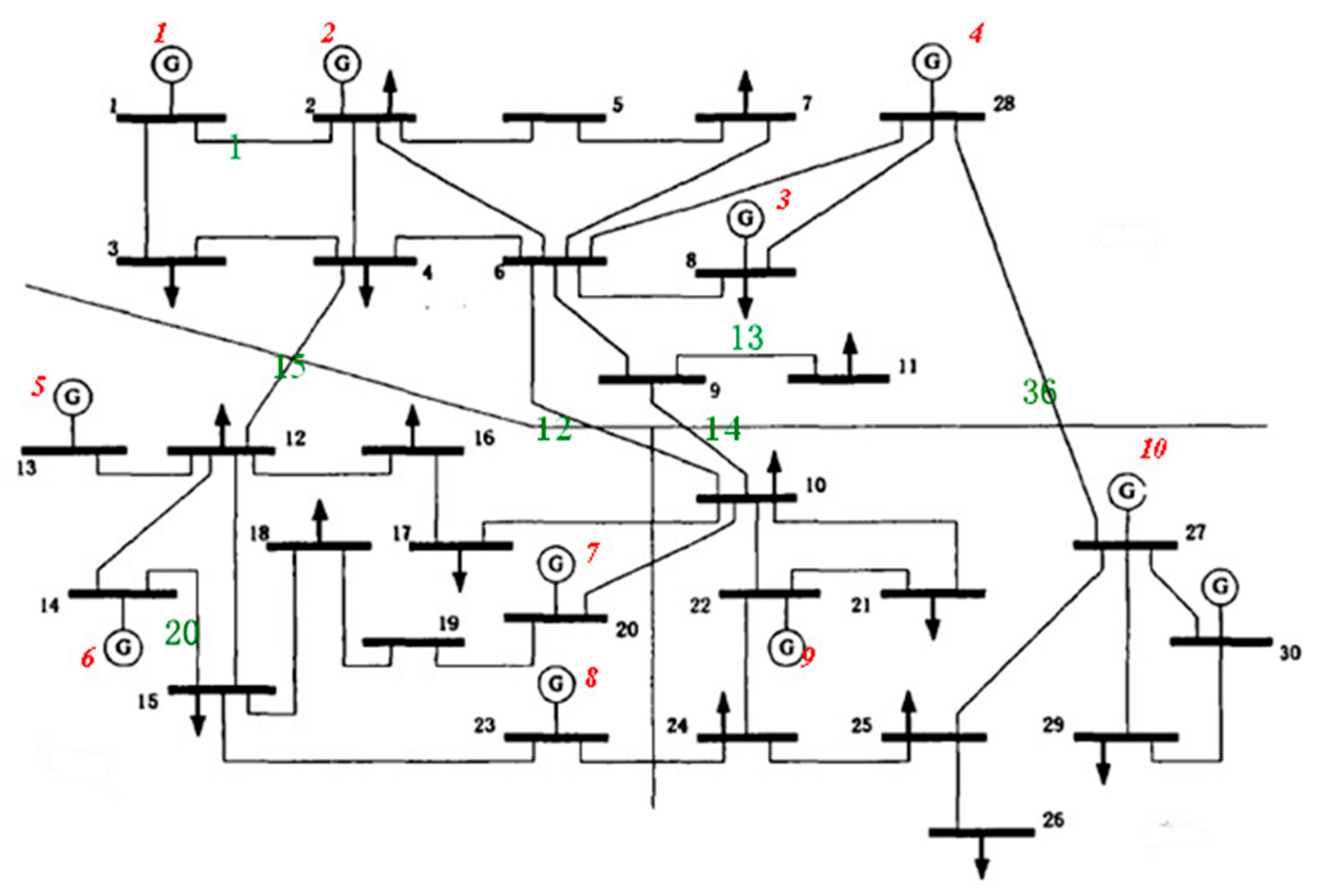
M3	239.88

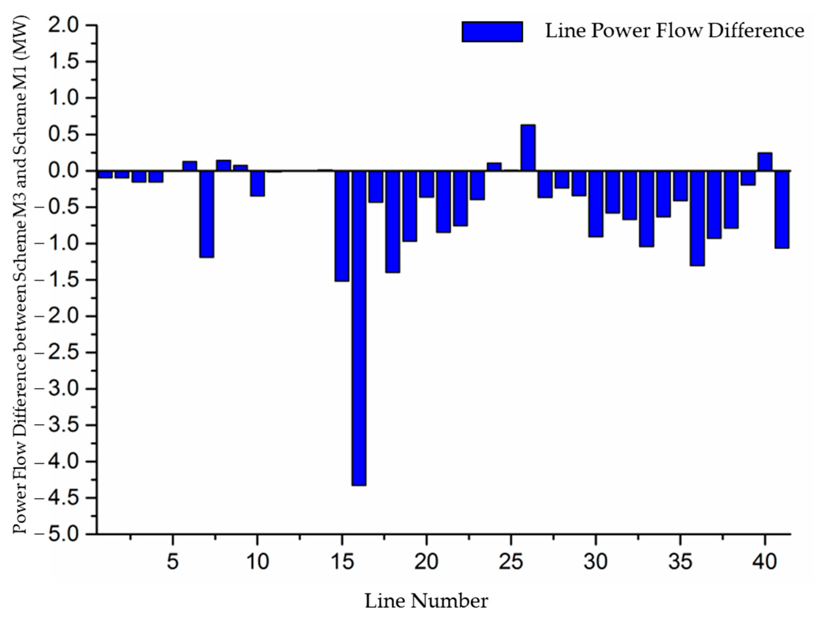
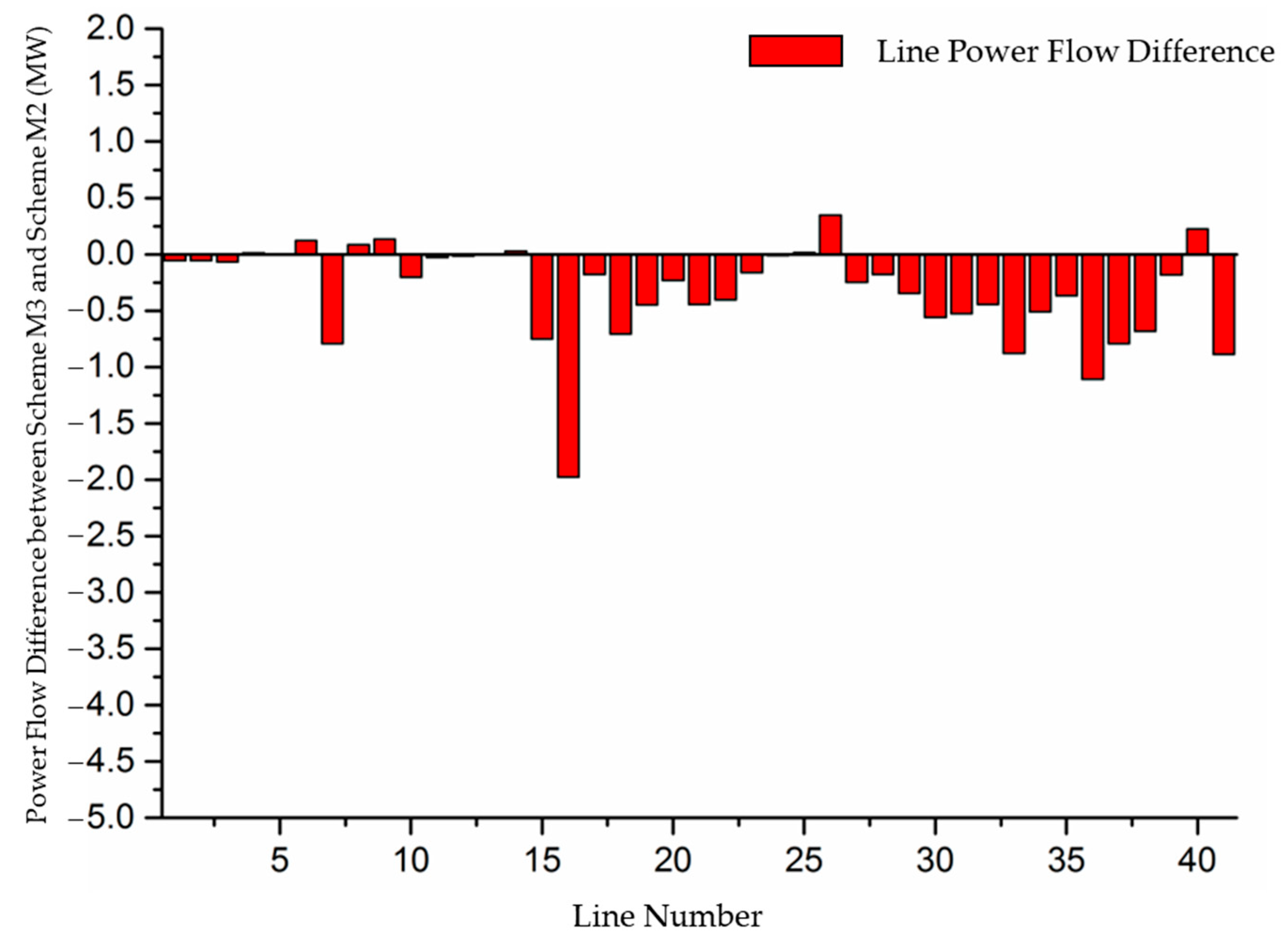
, Scheme M3 reduces the total system load by 1.84% compared with Scheme M1 and 0.81% compared with Scheme M2, highlighting the effectiveness of the proposed full-cost electricity pricing model in improving demand-side responsiveness. The networking of IEEE 30 bus system is shown in Figure 5. Figure 6 and Figure 7 illustrate the differences in power flow across the three schemes. Scheme M3 results in an overall reduction in system power flow, driven by more refined price signals. For transmission lines near generation centers (e.g., lines 1, 6, 8, 9, 24, 26, and 40), the power flow reduction is minimal, and in some cases, it even increases, reflecting a more balanced redistribution of resources. In contrast, transmission lines farther from generation centers (e.g., lines 7, 15, 16, 18, 36, 37, and 38) show a significant reduction in power flow, indicating the effectiveness of Scheme M3 in alleviating transmission burdens on long-distance corridors. A comparison of Figure 3 and Figure 6 and Figure 3 and Figure 7 demonstrates that the security-constrained economic dispatch model based on full-cost electricity pricing significantly reduces transmission congestion risks compared with traditional marginal pricing models, while further optimizing power flow allocation relative to the postage stamp method. By rationally allocating fixed transmission costs, the proposed model ensures that full-cost electricity prices reflect the true cost of electricity consumption at each node, incentivizing demand-side adjustments. This results in a redistribution of power flow, shifting transmission burdens from long-distance lines to those closer to generation centers, establishing a “near-high far-low” power flow pattern that enhances grid efficiency and the economic viability of transmission investments.

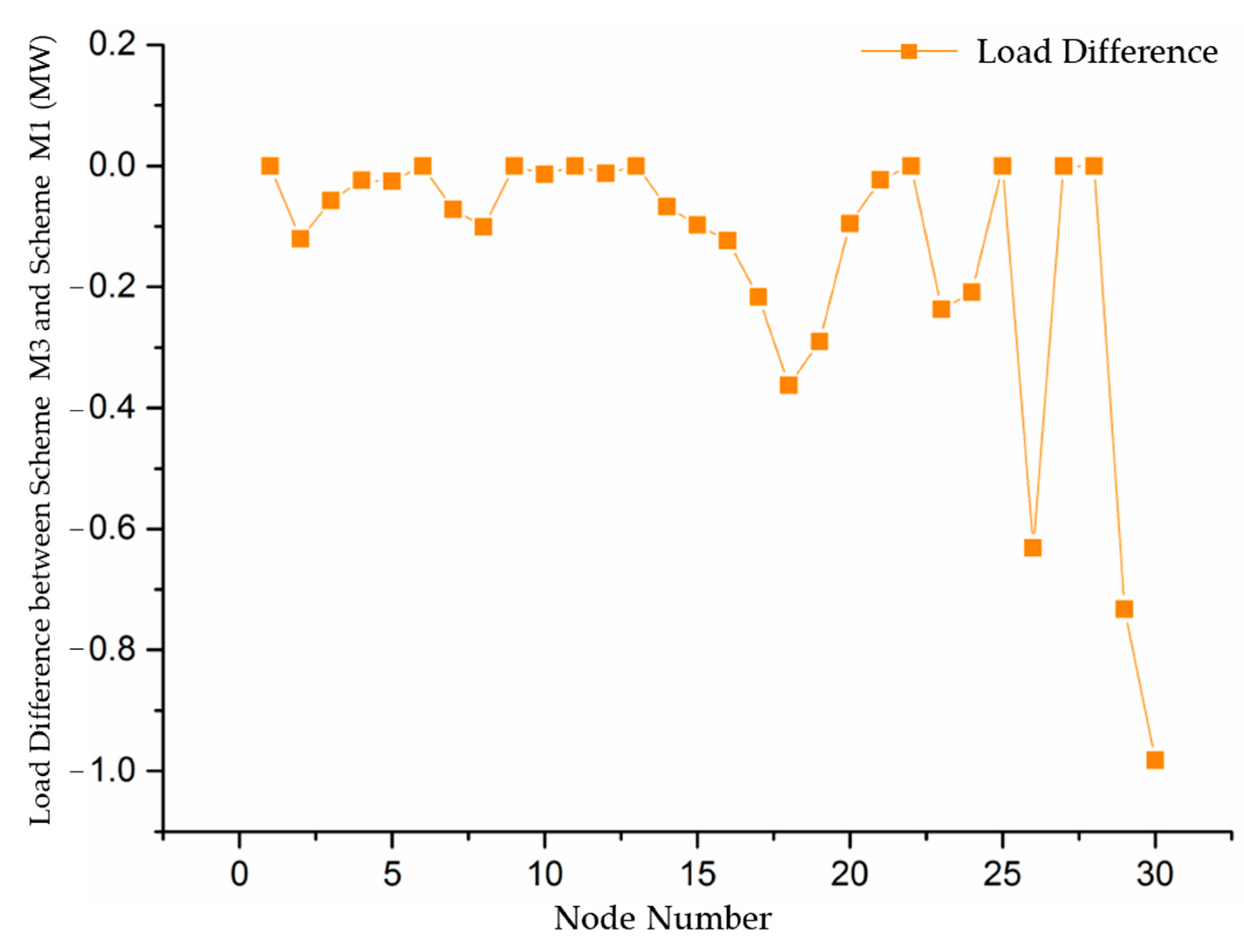
Figure 8 shows the load differences between Scheme M3 and Scheme M1, reflecting the impact of the two schemes on load. Scheme M1 does not consider fixed transmission costs, resulting in incomplete price signals and insufficient load response. In contrast, Scheme M3, based on full-cost electricity pricing, encourages greater load-side response to reduce electricity costs, leading to an overall decrease in load. Nodes closer to generation centers (e.g., nodes 1, 5, 28) show minimal load variation, while nodes farther from generation centers (e.g., nodes 18, 26, 29) experience significant load reductions due to higher transmission cost allocation. 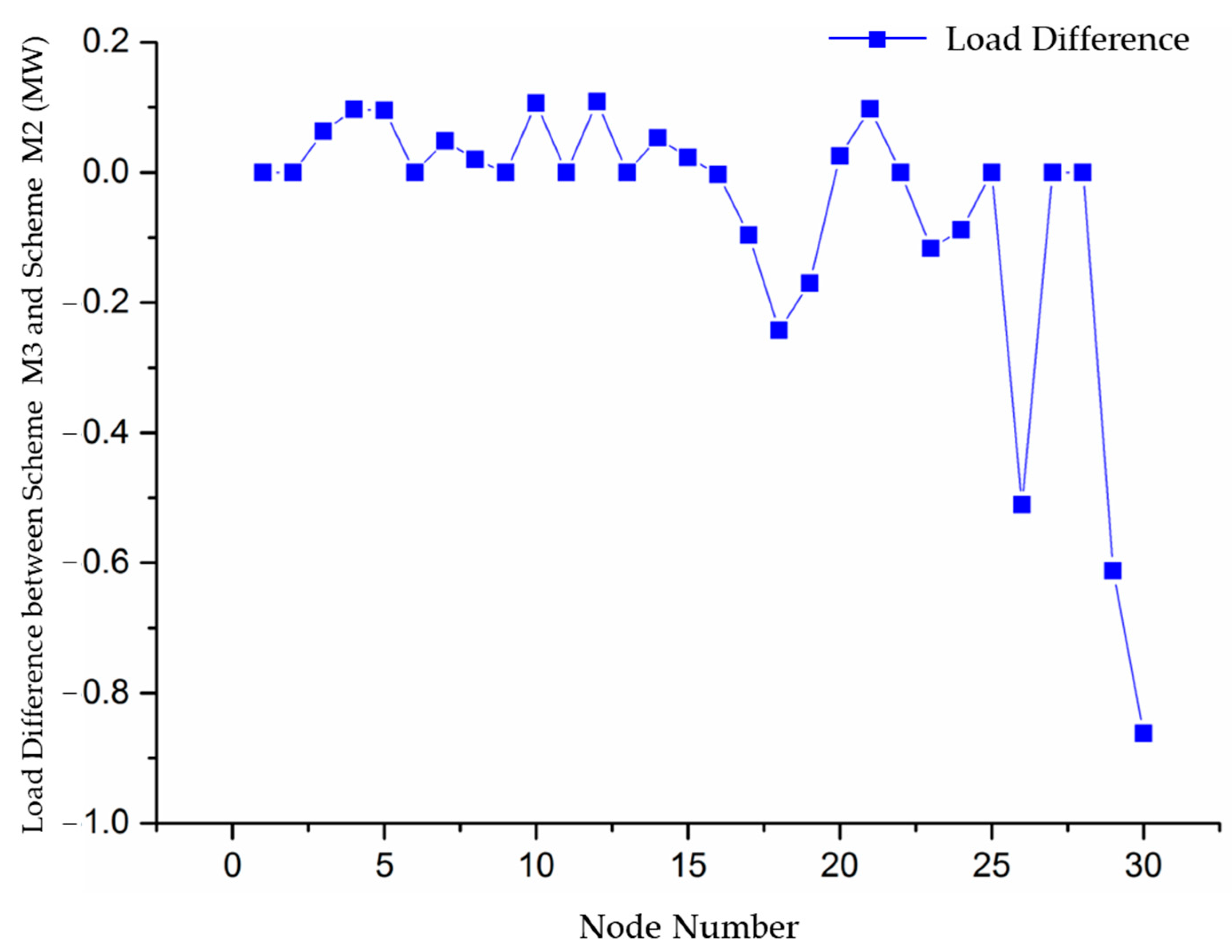Figure 9 illustrates the load differences between Scheme M3 and Scheme M2. Although Scheme M2 considers fixed transmission costs, the postage stamp method fails to reflect regional differences, leading to higher load reductions at nodes near generation centers. In contrast, distant nodes, with lower cost allocation, show less load response compared with Scheme M3. In conclusion, the load differences highlight that full-cost electricity pricing can accurately reflect the varying electricity costs at different nodes, thereby optimizing load distribution and enhancing load-side responsiveness.

Table 3. Comparison of full-cost electricity prices.

Node Number	Scheme M1 ($/MWh)	Scheme M2 ($/MWh)	Scheme M3 ($/MWh)	Node Number	Scheme M1 ($/MWh)	Scheme M2 ($/MWh)	Scheme M3 ($/MWh)
1	357.48	357.48	383.79	16	394.37	377.33	377.77
2	391.10	374.07	374.15	17	394.51	377.48	391.26
3	393.43	376.40	367.42	18	394.41	377.37	411.99
4	393.83	376.80	363.03	19	394.46	377.43	401.74
5	404.22	387.19	373.59	20	394.48	377.46	373.89
6	360.62	360.62	369.38	21	394.57	377.54	363.63
7	398.73	381.70	374.80	22	360.34	360.35	370.58
8	394.84	377.81	374.98	23	394.41	377.38	394.07
9	360.45	360.45	360.88	24	394.54	377.50	390.14
10	394.58	377.54	362.37	25	360.42	360.42	405.59
11	360.45	360.45	360.44	26	394.64	377.61	450.58
12	394.22	377.19	361.73	27	360.49	360.49	423.21
13	360.00	360.00	360.00	28	360.61	360.41	376.65
14	394.27	377.24	369.71	29	394.71	377.67	465.14
15	394.31	377.28	374.04	30	394.71	377.67	500.79

lists the nodal electricity prices under the three schemes. Overall, Scheme M1 has the highest electricity prices, followed by Scheme M2, and Scheme M3 has the lowest prices. The main reason is that Scheme M1 incorporates all fixed transmission costs into the electricity prices, while Scheme M2 only includes effective transmission costs. Scheme M3 uses the power flow tracing method to allocate fixed transmission costs, leading to a significant increase in electricity prices at nodes farther from generation centers, reflecting the principle of “costs borne by beneficiaries”. At nodes with long supply–demand distances, full-cost electricity prices rise significantly before congestion occurs. Combined with the power flow difference maps, it can be observed that the power flow on remote transmission lines decreases, helping to prevent line congestion. Furthermore, the load difference maps in Figure 3 and Figure 7 and Figure 3 and Figure 8 show that nodes with greater price increases exhibit a more pronounced reduction in load response.

In summary, the proposed method integrates transmission costs into full-cost electricity pricing and considers fixed transmission costs in economic dispatch and demand response, ensuring a more accurate reflection of grid resource utilization. By linking transmission investment returns to actual grid usage, it promotes rational and efficient grid investment.

To further validate its effectiveness, the IEEE 118-bus system with 54 generators and 186 transmission lines is used for analysis.

Table 4. Total cost comparison in IEEE 118-bus system network.

Scheme	Total Generation Cost ($)	Total Transmission Cost ($)	Total Consumption Cost ($)
M1	152,885.8	20,600.7	173,486.5
M2	151,803.5	13,056	164,859.5
M3	151,794.6	12,044	163,838.6

compares generation, transmission, and electricity consumption costs under the three schemes. Scheme M1 has the highest transmission cost, while Scheme M3, better reflecting actual grid utilization, further reduces it. Scheme M1’s generation cost is slightly higher due to weaker user response and lower cost savings. Scheme M3 achieves the lowest total electricity cost, highlighting its effectiveness in optimizing demand response.

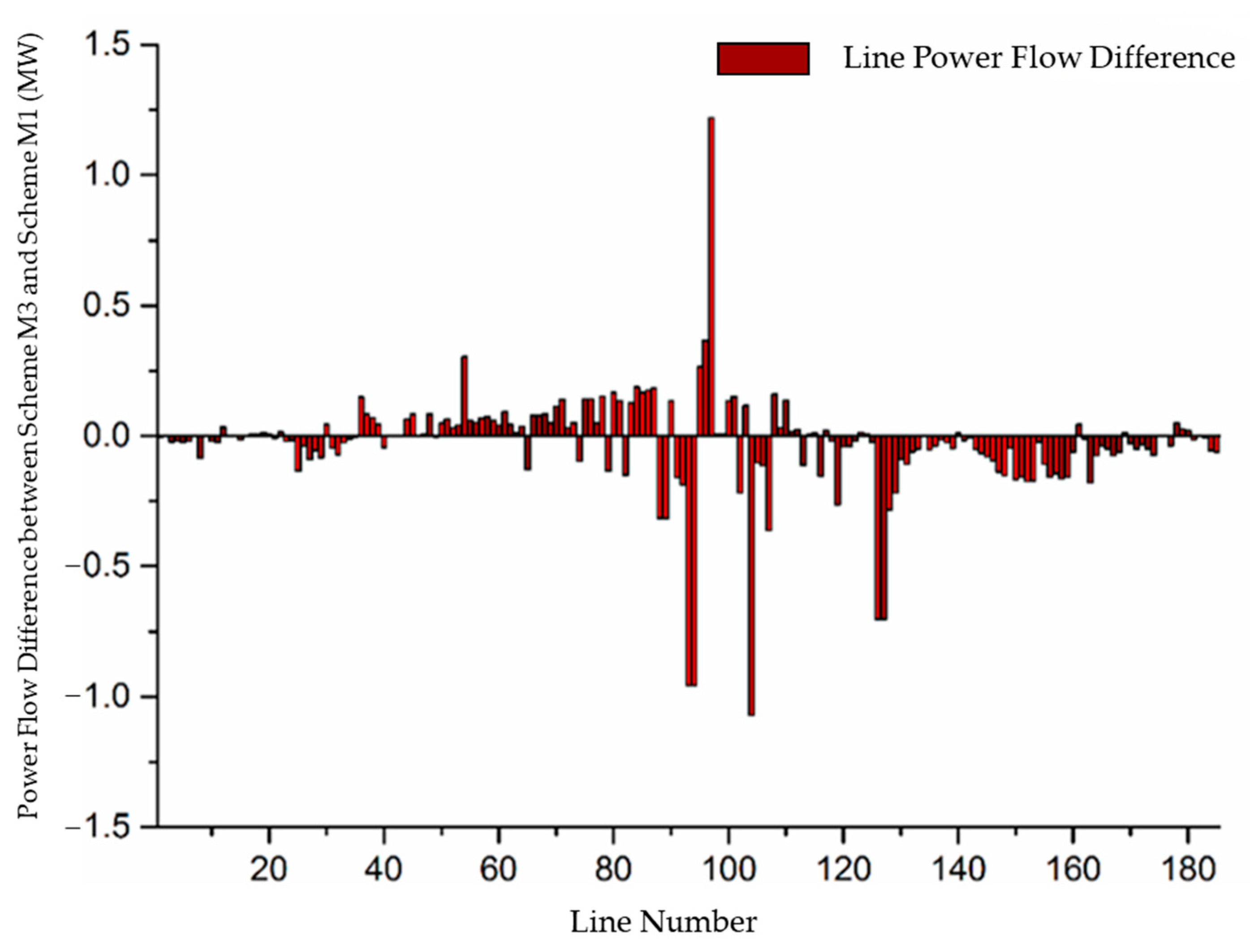
Figure 10 presents the power flow differences between Scheme M1 and Scheme M3. Overall, Scheme M3 results in slightly lower total power flow. Near generation lines (e.g., lines 54, 95, and 97) experience higher flow, while remote lines (e.g., lines 93, 94, and 126) show significant reductions, indicating a shift of power flow toward generation centers under the proposed dispatch model.

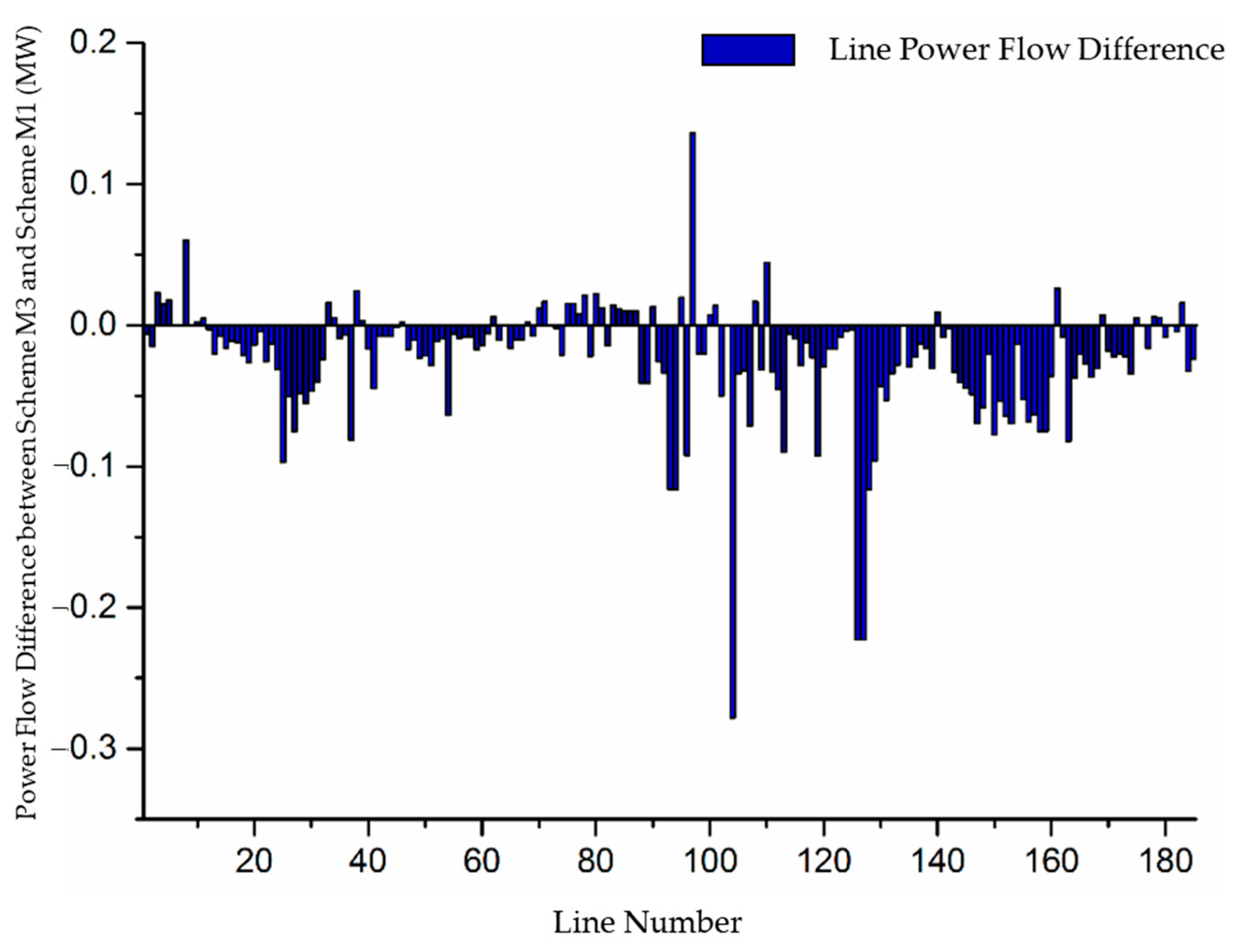
Figure 11 presents the power flow differences between Scheme M2 and Scheme M3. Overall, Scheme M3 results in lower total power flow compared with Scheme M2. Near generation lines (e.g., lines 8, 97, and 110) exhibit higher power flow in Scheme M3, while remote lines (e.g., lines 94, 104, and 127) show significant reductions, further highlighting the effectiveness of the proposed model in redistributing power flow toward generation centers.

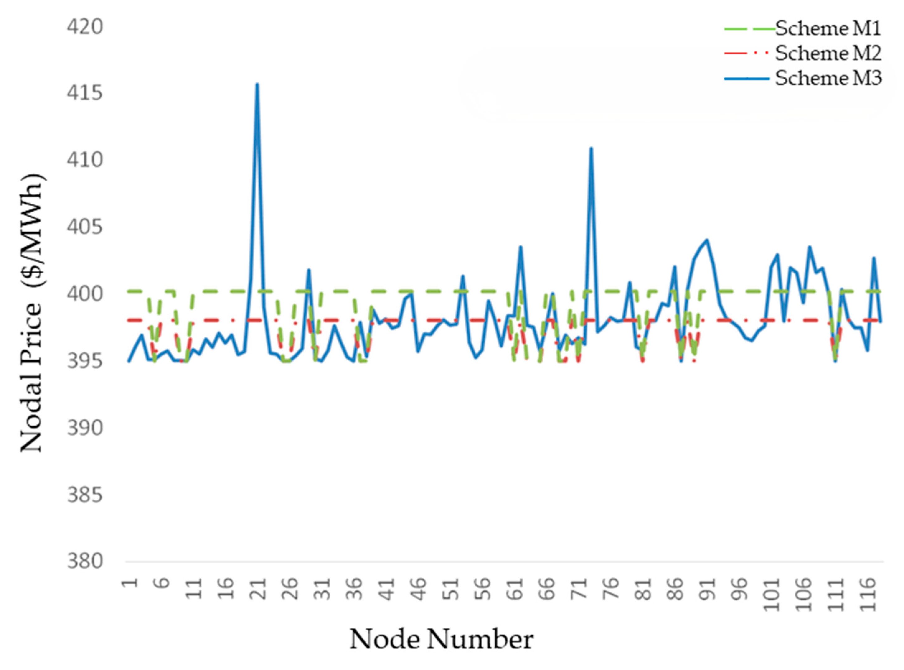
Figure 12 compares nodal electricity prices under the three schemes. Scheme M1 has the highest average price, followed by Scheme M2, while Scheme M3 results in lower prices at most nodes. Schemes M1 and M2 yield uniform prices due to the postage stamp method, whereas Scheme M3 increases prices at remote nodes (e.g., nodes 22, 74, and 92), effectively capturing spatial consumption differences and enhancing demand response incentives.

To better illustrate the differences among the three pricing strategies,

Table 5. Comparison of pricing strategies.

Pricing Scheme	Fairness	Price Signal Accuracy	Congestion Management	Computational Complexity
M1 (Traditional Nodal Pricing)	Low	Limited, does not reflect fixed transmission costs	No congestion differentiation	Low
M2 (Fixed Cost Allocation without Power Flow Tracing)	Medium	Considers transmission costs but lacks effective allocation	Partial congestion differentiation	Medium
M3 (Proposed Power Flow Tracing)	High	Accurately reflects transmission cost based on grid utilization	Effectively manages congestion	Moderate

summarizes their key characteristics.

These results confirm that M3 provides the most equitable and efficient cost allocation, making it the most practical pricing strategy.

3.4. Application and Validation of the Model in Large-Scale Power Systems

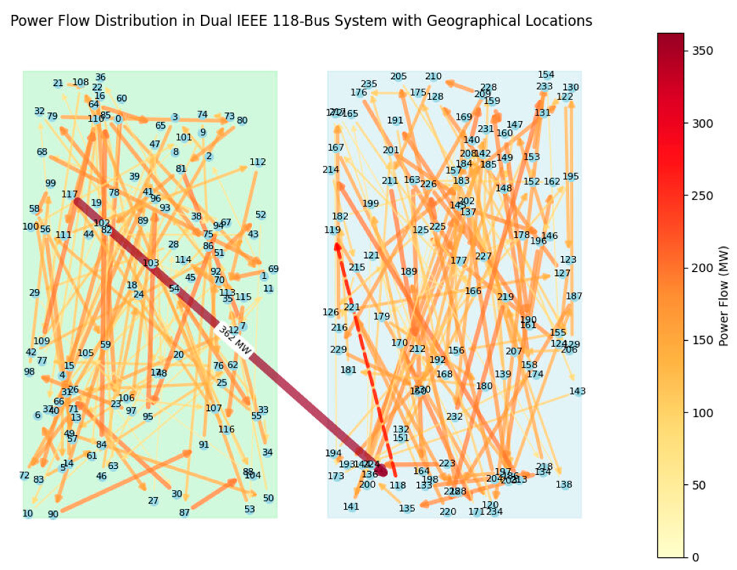
To evaluate the computational feasibility and performance of the proposed full-cost electricity pricing model, a dual IEEE 118-bus system is utilized to simulate inter-provincial power trading. This system consists of 236 nodes, 108 generators, and 392 transmission lines, with a single tie line connecting the two regions to enable controlled power flow exchanges. Province A (nodes 1–118) and Province B (nodes 119–236) have asymmetric parameters, meaning that their generation costs, transmission constraints, and power demand distributions vary significantly. This asymmetry better reflects real-world inter-provincial power trading conditions and allows for testing the effectiveness of the proposed pricing model under different grid configurations. By analyzing the model’s ability to track power flow and allocate transmission costs fairly in this large-scale system, we assess its computational feasibility and scalability for real-world applications.

To examine the computational feasibility of the proposed model, we compare the computation time and convergence behavior across different system sizes. The analysis includes IEEE 30-bus, IEEE 118-bus, and dual IEEE 118-bus systems, allowing for a comprehensive evaluation of the model’s scalability. The results indicate that the computation time scales quadratically with the network size, yet the model remains computationally feasible even in the largest test case.

The results in

Table 6. Comparison time for different test systems.

Test System	Number of Nodes	Number of Generators	Number of Transmission Lines	Average Iterations	Computation Time (s)
IEEE 30-bus	30	6	41	8	0.35
IEEE 118-bus	118	54	186	14	1.42
Dual IEEE 118-bus	236	108	392	18	3.91

show that the model successfully converges within 20 iterations across all tested networks. The computation time remains within acceptable limits, confirming that the proposed full-cost pricing model is feasible for large-scale grid applications.

To further validate the performance of the proposed pricing model, Figure 3 visually represents the power flow distribution in the dual IEEE 118-bus system using color gradients and line thickness to indicate the magnitude of power flow across transmission lines. The node numbers are clearly labeled, ensuring a precise identification of different grid locations.

To enhance geographical context, a geographical distribution map of the two provinces (Province A and Province B) is incorporated at the bottom of the figure. This map illustrates the spatial distribution of generator units corresponding to each node, providing insights into the regional allocation of power generation and consumption. Additionally, layered annotations are used to distinguish between Province A and Province B, ensuring that the regional boundaries of the two interconnected grids are clearly marked. This visual enhancement aids in understanding how power is transmitted and exchanged between the two provinces, offering an intuitive representation of regional power flow patterns.

The analysis in Figure 13 demonstrates that the tie line between Province A and Province B plays a crucial role in facilitating inter-provincial power exchanges, highlighting the necessity of an accurate transmission cost allocation mechanism. Additionally, congestion-prone transmission lines exhibit higher utilization, emphasizing the importance of a fair and dynamic cost allocation approach. The proposed pricing model effectively addresses these challenges by proportionally distributing transmission costs based on actual power flow, ensuring that cost allocation reflects real grid resource utilization and promotes more efficient power transactions.

3.5. Comparative Analysis of the Proposed Full-Cost Electricity Pricing Model and Existing Pricing Methods

To evaluate the effectiveness of the proposed full-cost electricity pricing model based on power flow tracing (M3), we compare it with three existing electricity pricing models: traditional nodal marginal pricing, postage stamp method, and uncertain-flow-based pricing models. The comparison focuses on key performance metrics, including fairness, price signal accuracy, congestion sensitivity, investment efficiency, and computational feasibility.

The key performance indicators used for evaluating the proposed pricing model include fairness, which measures how proportionally transmission costs are allocated based on actual power usage by comparing allocated costs with ideal power flow-based costs; price signal accuracy, which assesses how well the model reflects real grid operation costs by analyzing deviations between theoretical and model-generated nodal prices; congestion sensitivity, which determines whether the model effectively differentiates costs based on transmission congestion by examining cost variations in heavily loaded lines; investment efficiency, which evaluates whether the pricing model encourages rational transmission investments by linking cost allocation to actual grid utilization and comparing model-driven investment decisions with optimal grid expansion strategies; and computational feasibility, which reflects the model’s suitability for real-time market applications by measuring the number of iterations required for convergence and assessing its relative computational complexity.

The results in

Table 7. Comparison time for different pricing models.

Pricing Model	Fairness (%)	Price Signal Accuracy (%)	Congestion Sensitivity (%)	Investment Efficiency (%)	Computational Complexity (Relative Scale)
Traditional Nodal Pricing	45.2	78.4	60.2	65.7	1 (baseline)
Postage Stamp Method	60.7	82.1	82.1	70.3	1.2
Uncertain Flow-Based Pricing	85.4	88.9	85.4	91.2	3.8 (computationally intensive)
M3 (Power Flow Tracing)	91.8	91.6	92.3	87.9	1.5 (efficient for real-time pricing)

highlight the advantages of the proposed full-cost electricity pricing model based on power flow tracing (M3) over existing pricing methods. In terms of fairness, M3 achieves the highest score by dynamically allocating transmission costs based on real-time power flow, ensuring proportional cost distribution, whereas traditional nodal pricing ignores fixed transmission costs, and the postage stamp method applies uniform allocation regardless of actual grid usage. For price signal accuracy, M3 effectively integrates both marginal generation and transmission costs, producing more precise economic signals compared with the distortions seen in postage stamp pricing and the partial accuracy of nodal pricing. Regarding congestion sensitivity, M3 dynamically adjusts cost allocation in response to transmission constraints, significantly outperforming nodal and postage stamp pricing, which lack congestion-based cost differentiation. In investment efficiency, M3 provides superior pricing signals for rational transmission investment, unlike traditional models that may lead to over- or underinvestment due to misaligned cost allocation. In computational feasibility, M3 strikes a balance between accuracy and efficiency, avoiding the excessive computational burden of uncertain flow-based pricing while maintaining a high level of pricing precision, making it more practical for real-time electricity markets.

3.6. Sensitivity Analysis

Changes in fuel costs and transmission line capacity significantly impact electricity pricing and power system operation efficiency. To ensure the robustness of the proposed full-cost electricity pricing model (M3), a sensitivity analysis is conducted to assess how variations in these parameters affect nodal electricity prices, congestion costs, and total system costs.

The analysis evaluates the sensitivity of the proposed model under two key scenarios: a 10% increase in fuel costs and a 15% reduction in transmission line capacity, using the IEEE 118-bus and dual IEEE 118-bus systems as test cases. The impact is measured through three key indicators: electricity price change rate (EPCR, %), which quantifies the percentage change in average nodal electricity prices; congestion cost variation (CCV, %), which assesses the increase in congestion-related transmission costs; and total system cost change (TSCC, %), which reflects the overall effect on system operation costs, including both generation and transmission expenses.

The results in

Table 8. Impact of fuel cost and transmission capacity changes on electricity prices and system costs.

Scenario	EPCR (%)	CCV (%)	TSCC (%)
Base Case	-	-	-
Fuel Cost +10%	6.5	0.8	5.2
Transmission Capacity −15%	4.8	9.1	7.4

indicate that a 10% increase in fuel costs leads to a 6.5% rise in average nodal electricity prices, with more pronounced effects in regions dependent on thermal generation. In contrast, a 15% reduction in transmission line capacity results in a 9.1% increase in congestion costs and a 7.4% rise in total system costs, highlighting the critical role of transmission infrastructure in electricity pricing.

These findings confirm that M3 effectively captures the impact of economic and technical variations, ensuring that price signals remain accurate and reflective of real grid conditions. The proposed model dynamically adjusts cost allocations in response to fuel cost fluctuations and congestion constraints, making it a reliable and adaptable pricing mechanism for electricity markets.

3.7. Regression-Based Forecasting Model for Electricity Pricing

To further enhance the quantitative capabilities of the proposed full-cost electricity pricing model (M3), a regression-based forecasting model is developed to predict how key economic and operational parameters influence nodal electricity prices. Given that electricity pricing is affected by multiple interdependent factors, such as fuel cost variations, demand response, and transmission network constraints, establishing a mathematical relationship between these factors and nodal prices allows for improved market predictability and pricing adjustments.

The forecasting model examines how variations in fuel costs, demand response, and transmission capacity impact electricity pricing. A multiple linear regression model is formulated to capture these relationships as follows:

$${\pi }_k={\beta }_0+{\beta }_1{f}_k+{\beta }_2{D}_{Lk}+{\beta }_3{F}_k+ϵ$$

(23)

where ${\pi }_k$ is the nodal electricity price at node $k$ ($/MWh), serving as the dependent variable; $f_k$ represents fuel costs at node $k$ ($/MWh), reflecting fluctuations in generation expenses; $D_{Lk}$ denotes demand response impact at node $k$ (MW), capturing consumer load adjustments in response to price signals; $F_k$ represents transmission capacity constraints (MW), indicating the available transmission limits affecting congestion and price formation; ${\beta }_0$, ${\beta }_1$, ${\beta }_2$, and ${\beta }_3$ are regression coefficients estimated from empirical data; $ϵ$ accounts for unmodeled market variations and external influences.

The regression model is developed and validated using simulation data from the IEEE 118-bus system and the dual IEEE 118-bus system, incorporating multiple scenarios with fuel cost increases of 10%, varying levels of demand response participation, and a 15% reduction in transmission capacity to simulate congestion effects. The dataset ensures a diverse range of market conditions, improving the robustness of the forecasting model.

The results presented in

Table 9. Regression model performance metrics.

Test System	Mean Absolute Error (MAE)	Root Mean Square Error (RMSE)	R2 Score
IEEE 118-bus	3.21	4.05	0.91
Dual IEEE 118-bus	5.08	6.38	0.88

confirm that the regression model achieves high predictive accuracy, with R² values exceeding 0.88 across all test cases, indicating a strong correlation between the selected input parameters and nodal electricity prices. The analysis demonstrates that fuel cost variations significantly impact electricity prices, with a regression coefficient of β₁ = 0.63, meaning that a 10% increase in fuel costs leads to a 6.3% rise in average nodal prices. Additionally, demand response participation shows a strong negative correlation (β₂ = −0.47) with nodal prices, suggesting that higher consumer load adjustments effectively mitigate price volatility. Furthermore, transmission constraints ($C_k$) play a critical role in congestion pricing, as reducing transmission capacity leads to steeper price differentials across nodes, emphasizing the need for effective congestion management in cost allocation. These findings validate that the proposed model accurately captures market dynamics and provides reliable forecasting of electricity pricing trends.

The regression-based forecasting model enhances the practical applications of the full-cost electricity pricing framework (M3) by enabling real-time price adjustments, allowing market operators to anticipate fuel cost fluctuations and congestion-related price variations, thereby improving market efficiency. Additionally, it supports long-term transmission investment planning by providing insights into future congestion pricing trends, ensuring that infrastructure expansion decisions are data-driven and economically justified. Furthermore, the model strengthens demand response strategies, assisting consumers in optimizing electricity consumption based on expected price movements, leading to a more balanced and efficient power system.

These results validate that the proposed full-cost pricing model is not only a cost allocation mechanism but also a robust predictive tool for electricity markets. By accurately integrating economic and technical parameters into pricing forecasts, the model ensures that pricing signals remain fair, adaptive, and responsive to real-world grid conditions, making it a practical and scalable solution for dynamic electricity market operations.

4. Conclusions and Future Outlook

This study proposes a full-cost electricity pricing model (M3) based on power flow tracing, addressing key limitations in existing pricing methods. Compared with traditional nodal marginal pricing (M1) and the postage stamp method (M2), M3 achieves higher fairness, improved price signal accuracy, and better congestion management by dynamically allocating fixed transmission costs based on actual grid utilization. The model was validated using IEEE 118-bus and dual IEEE 118-bus test systems, demonstrating its capability to reflect real-world grid conditions and market dynamics.

The proposed model is also computationally efficient, converging within 20 iterations across all tested networks, making it suitable for real-time market applications. Furthermore, the sensitivity analysis confirms that fuel cost variations and load fluctuations significantly influence electricity pricing, highlighting M3’s adaptability as a dynamic and responsive pricing mechanism. The regression-based forecasting model further enhances its applicability by accurately predicting nodal price variations under different economic and technical conditions. Finally, the case study on the dual IEEE 118-bus system validates the feasibility of M3 in inter-provincial electricity trading, proving its capability to support large-scale power market operations.

Although M3 improves electricity pricing in terms of fairness, accuracy, and congestion management, several challenges remain in its practical implementation, particularly concerning demand-side response (DSR). Many electricity markets are regulated, which may limit price fluctuations and reduce the effectiveness of real-time price signals in influencing consumer behavior. Additionally, consumer inertia poses a challenge, as many users are not accustomed to adjusting electricity usage based on dynamic pricing strategies. Furthermore, the deployment of DSR relies on smart grid infrastructure, including automated demand management systems and real-time energy monitoring devices, which are not yet widely adopted in all regions. Future applications of M3 should consider these limitations to ensure effective implementation in diverse market environments.

Another promising direction for future research is the integration of AI-based optimization techniques with the full-cost electricity pricing model [22,23]. While this study employs a linear programming (LP)-based approach, we recognize the potential of genetic algorithms (GAs), ant colony optimization (ACO), and neural networks in handling complex nonlinear optimization problems, particularly in the presence of renewable energy uncertainty. AI-driven methods could enhance M3’s adaptability in large-scale systems, improve its real-time optimization capabilities, and potentially accelerate convergence. However, the trade-off between computational efficiency and solution accuracy remains a critical challenge. Future studies will explore the integration of heuristic optimization and AI techniques into M3, improving its applicability in dynamic electricity markets.

By addressing these challenges and incorporating advanced optimization techniques, M3 can be further enhanced to support real-time electricity market operations, promote efficient grid investments, and enable adaptive pricing mechanisms that align with evolving power system conditions.