Carbon Emission Prediction of Freeway Construction Phase Based on Back Propagation Neural Network Optimization

Abstract
1. Introduction
2. Materials and Methods
2.1. Carbon Emission Calculation Methodology
- Carbon emissions at the material production stage:
- Carbon emissions at the material transportation stage:
- Carbon emissions during the construction phase:
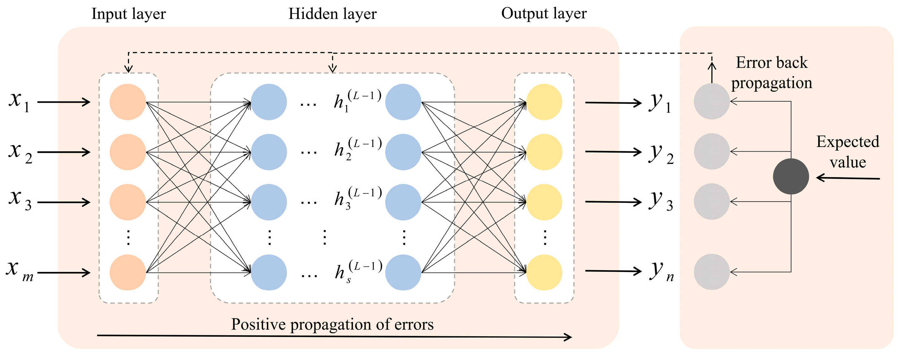
2.2. Neural Network Construction Method
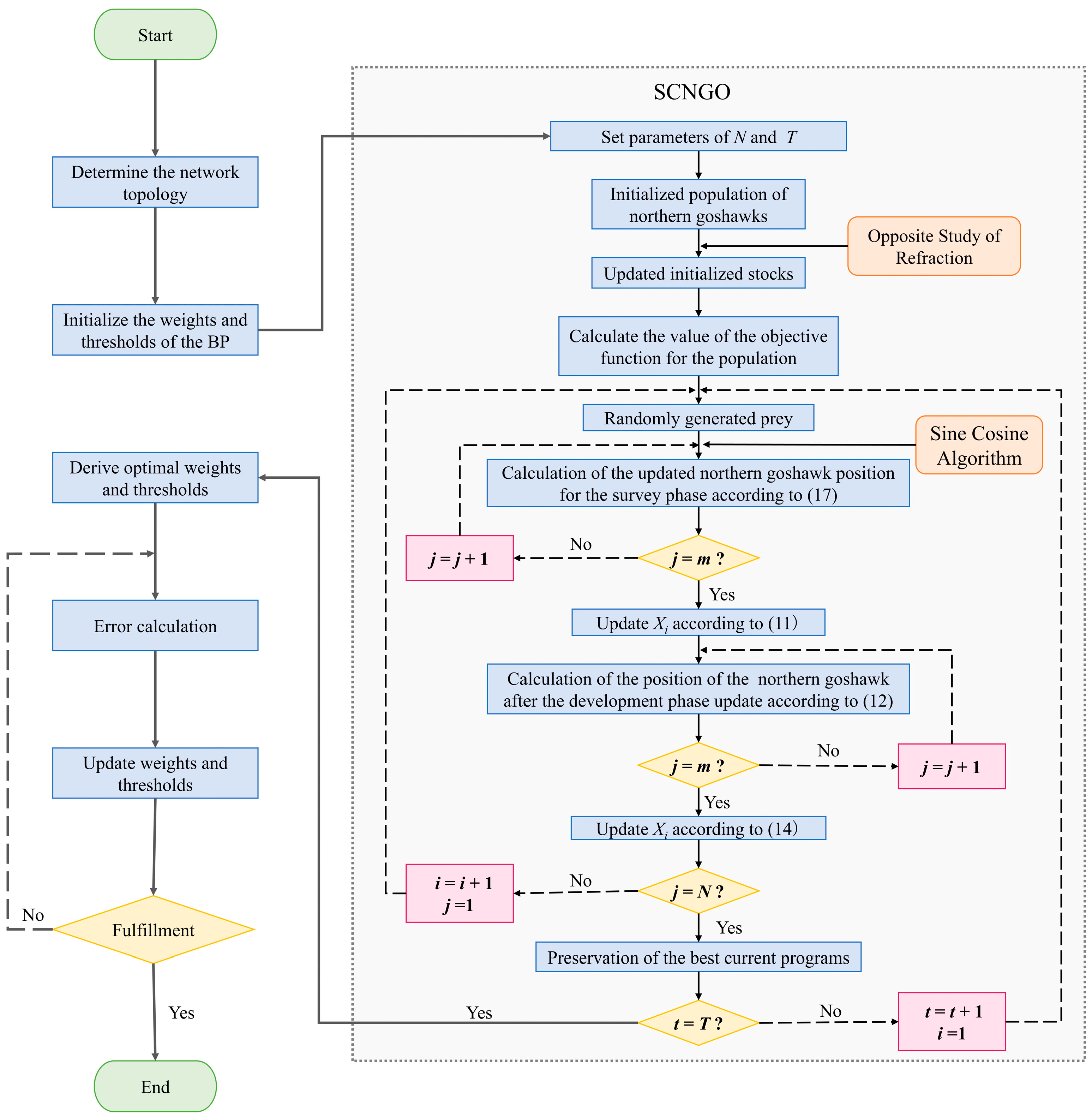
2.3. Optimization Methods for Neural Networks
2.3.1. Northern Goshawk Optimization
2.3.2. Improving the Northern Goshawk Optimization by Incorporating Multiple Strategies
- Introducing the Opposite Study of Refraction
- 2.
- Introducing the Sine Cosine Algorithm
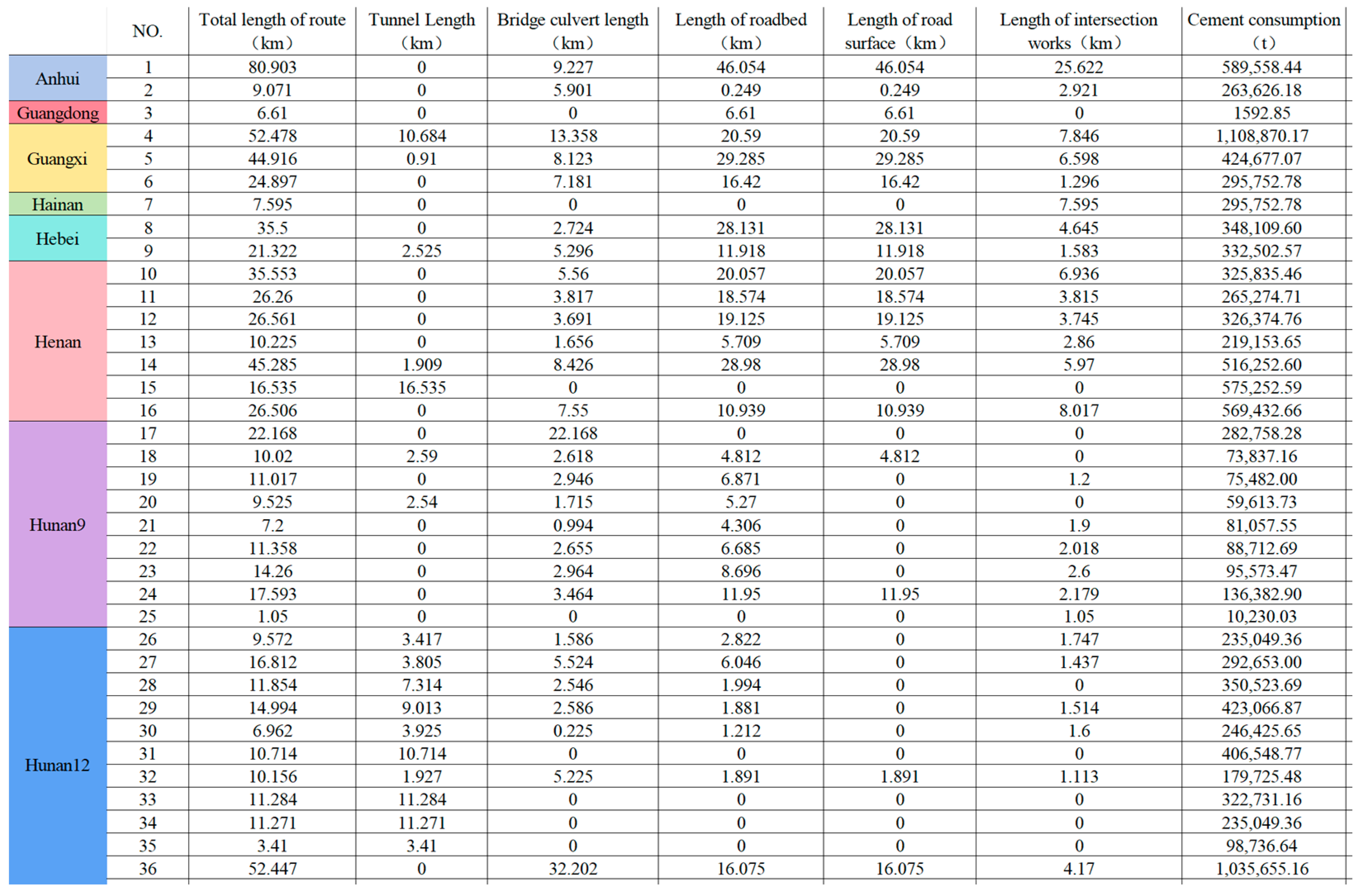
2.4. Data Sources
3. Model Predictions and Analysis of Results
3.1. Selection of Predictive Indicators
3.1.1. Selection of Relevant Variables
3.1.2. Predictive Indicator Identification
- Determining the study series
- 2.
- Dimensionless data processing
- 3.
- Calculation of correlation coefficients
- 4.
- Calculating correlation
- 5.
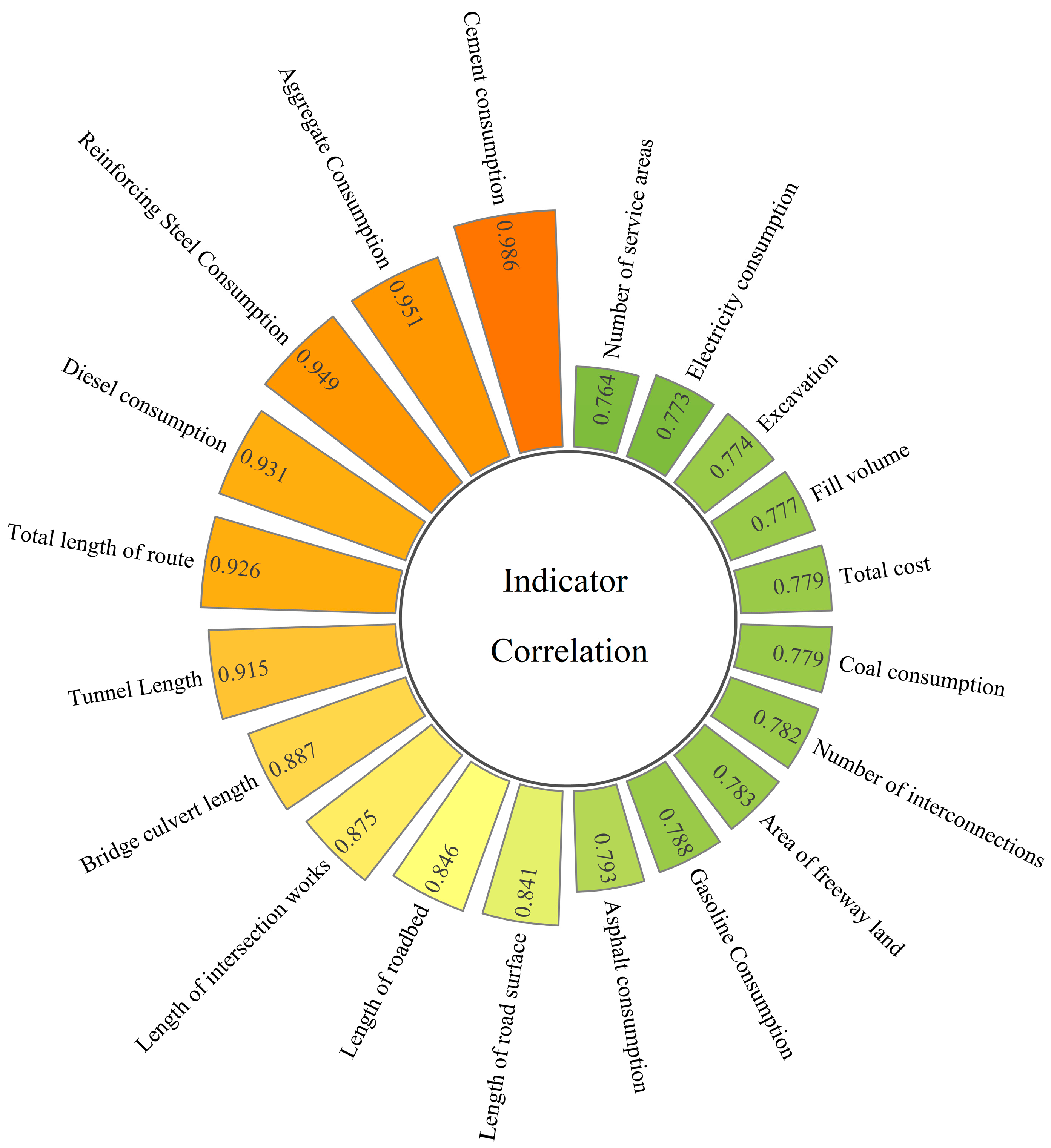
- Analysis of associated findings
3.2. Model Parameterization and Training
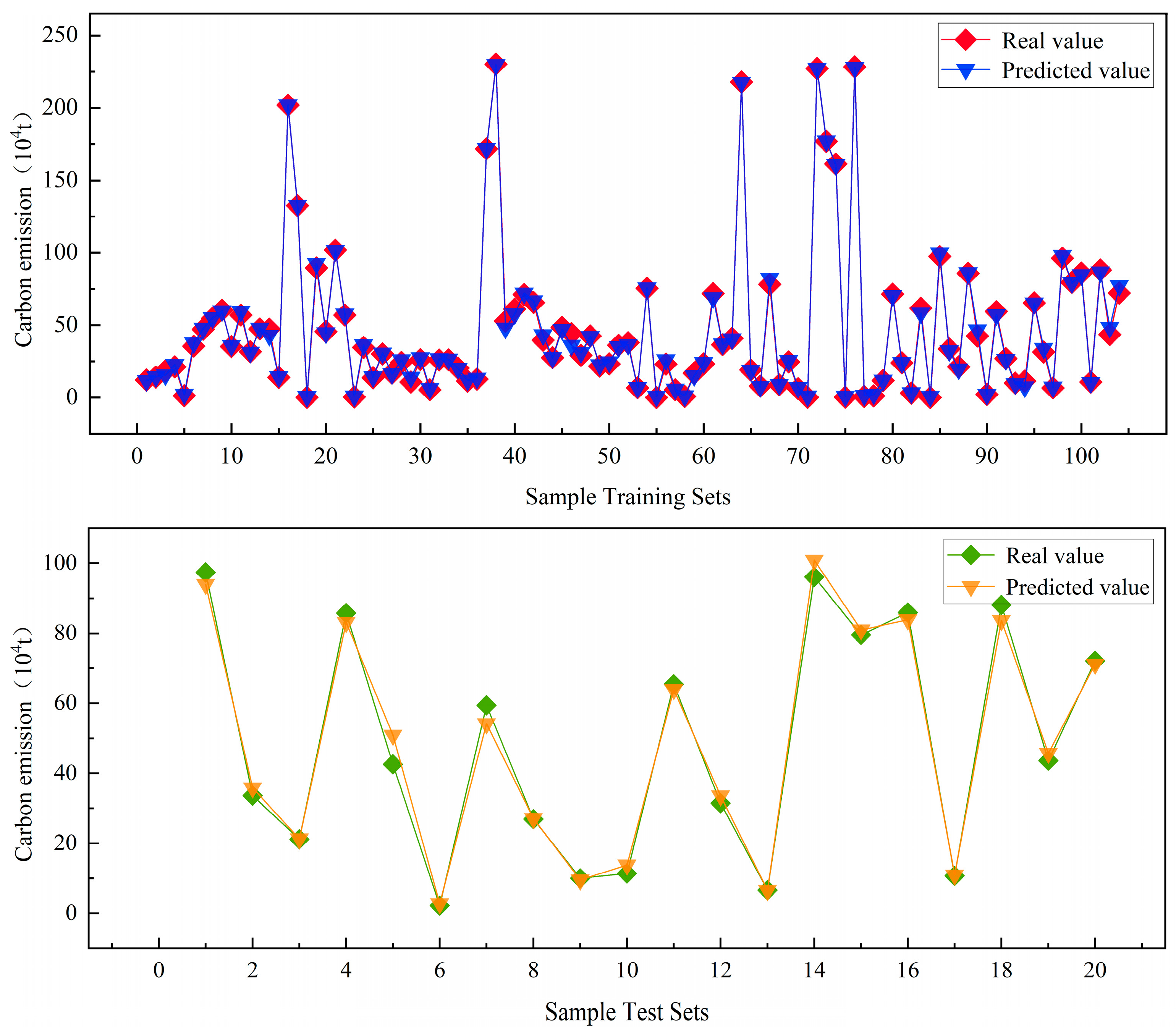
3.2.1. Carbon Emission Prediction Model Constructed Based on BP Neural Network
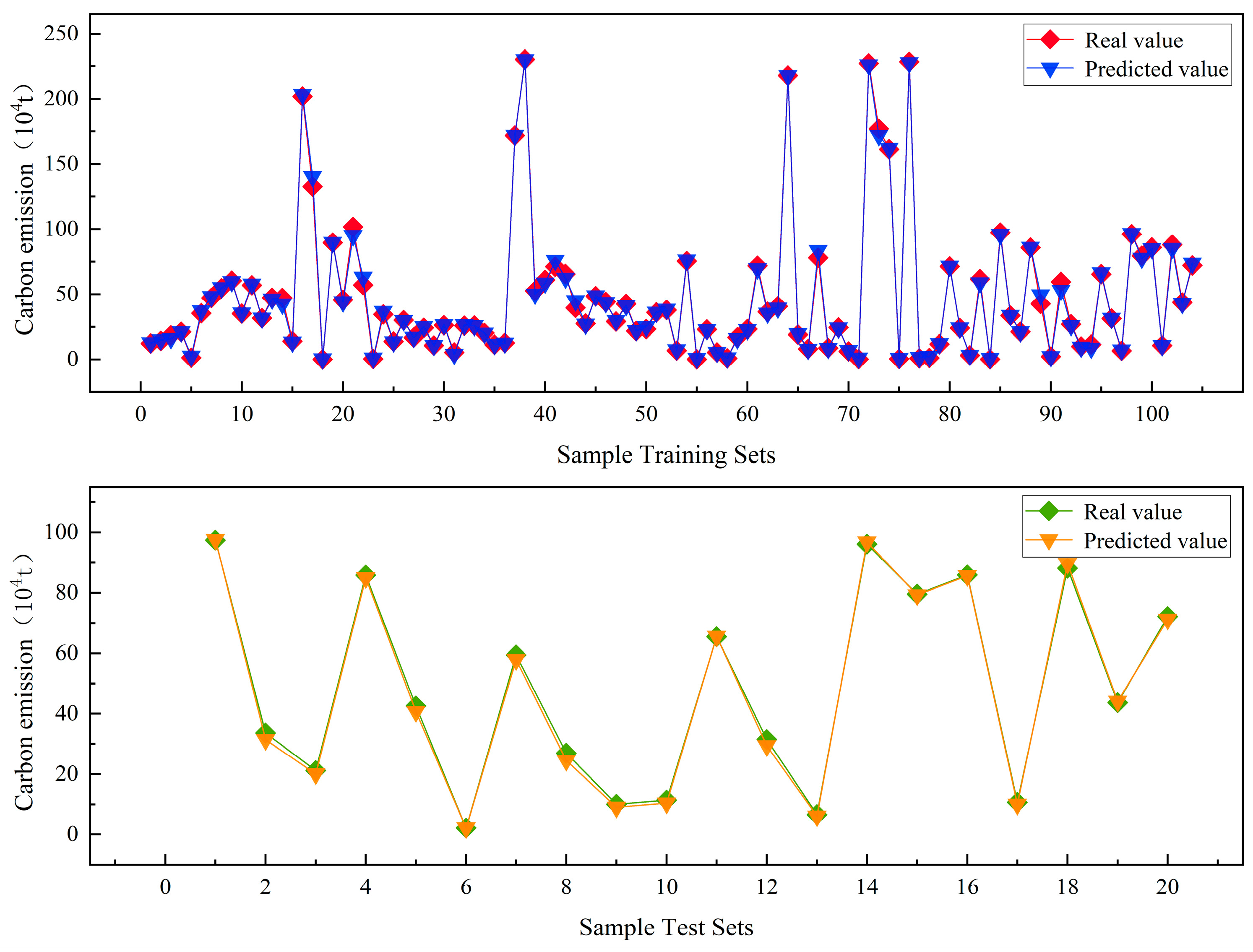
3.2.2. Carbon Emission Prediction Model Constructed Based on SCNGO Improved BP Neural Network
3.3. Performance Comparison of Different Network Models
3.4. Carbon Emission Projections for the Construction Phase of a Freeway
4. Conclusions
- The four materials of cement, crushed stone, steel reinforcement, and diesel exhibit substantial consumption during highway construction and have a strong correlation with carbon emissions. Similarly, tunnel length, bridge and culvert length, and intersection length, serving as key linear indicators in highway construction projects, are also closely related to carbon emissions.
- The optimization of the BP neural network through the integration of a multi-strategy improved northern goshawk optimization (SCNGO) algorithm yields significant results, which are primarily manifested in two aspects: a reduction in the maximum error value and a tightening of the error range. The predictions of the carbon emissions during the construction phase of different route schemes for actual highway projects, based on the SCNGO-BP prediction model, align closely with reality.
Author Contributions
Funding
Data Availability Statement
Conflicts of Interest
References
- Tarasova, O.A.; Braathen, G.O.; Barrie, L.A.; Suda, K.; Dlugokencky, E. The state of greenhouse gases in the atmosphere using global observations through 2008. EGU Gen. Assem. Conf. Abstr. 2010, 5, 23–28. [Google Scholar]
- Dangendorf, S.; Hay, C.; Calafat, F.M.; Marcos, M.; Piecuch, C.G.; Berk, K.; Jensen, J. Persistent acceleration in global sea-level rise since the 1960s. Nat. Clim. Change 2019, 9, 705–710. [Google Scholar]
- International Energy Agency. CO2 Emissions in 2022; IEA: Paris, France, 2023. [Google Scholar]
- Liu, Y. Study on the Theory and Calculation Methods of Carbon Dioxide Emission from the Highway Life Cycle Using ALCA. Ph.D. Thesis, Chang’an University, Xi’an, China, 2019. [Google Scholar]
- Zheng, Y.; Sun, W.; Du, S.; Zhu, L.; Huang, Y. Review of carbon emission accounting methods in coal enterprises. J. China Coal Soc. 2023, 49, 1143–1153. [Google Scholar]
- Li, Z.; Lu, W.; Pang, X.; Li, Y.; Bai, K.; Li, S.; Lu, Z.; Yao, S. Research and application of on-line monitoring system for CO2 emissions from thermal power enterprises. Clean Coal Technol. 2020, 26, 182–189. [Google Scholar]
- Liu, Y.; Li, Y.; Zhou, C.; Song, J.; Deng, H.; Du, E.; Zhang, N.; Kang, C. Overview of Carbon Measurement and Analysis Methods in Power Systems. Proc. CSEE 2024, 44, 2220–2236. [Google Scholar]
- Aggarwal, P.; Jain, S. Energy demand and CO emissions from urban on-road transport in Delhi: Current and future projections under various policy measures. J. Clean. Prod. 2016, 128, 48–61. [Google Scholar]
- Chen, S.S.; Mihara, K.; Wen, J.X. Time series prediction of CO2, TVOC and HCHO based on machine learning at different sampling points. Build. Environ. 2018, 146, 238–246. [Google Scholar]
- Khan, M.J.U.R.; Awasthi, A. Machine learning model development for predicting road transport GHG emissions in Canada. WSB J. Bus. Financ. 2019, 53, 55–72. [Google Scholar]
- Qu, Y.; Bai, H.; Xu, H. Scenario analysis-based transportation carbon emission forecasting study in Hubei Province. Environ. Pollut. Control 2010, 32, 102–105+110. [Google Scholar]
- Singh, M.; Dubey, R.K. Deep Learning Model Based CO2 Emissions Prediction Using Vehicle Telematics Sensors Data. IEEE Trans. Intell. Veh. 2023, 8, 768–777. [Google Scholar]
- Liu, H.; Hu, D. Construction and Analysis of Machine Learning Based Transportation Carbon Emission Prediction Model. Huan Jing Ke Xue 2024, 45, 3421–3432. [Google Scholar] [PubMed]
- Sun, W.; Jin, H.; Wang, X. Predicting and Analyzing CO2 Emissions Based on an Improved Least Squares Support Vector Machine. Pol. J. Environ. Stud. 2019, 28, 4391–4401. [Google Scholar]
- Li, Y.M.; Hu, H.D. Influential Factor Analysis and Projection of Industrial CO2 Emissions in China Based on Extreme Learning Machine Improved by Genetic Algorithm. Pol. J. Environ. Stud. 2020, 29, 2259–2271. [Google Scholar]
- Santero, N. Life Cycle Assessment of Pavements: A Critical Review of Existing Literature and Research; Lawrence Berkeley National Laboratory: Berkeley, CA, USA, 2018; DE-AC02-05CH11231. [Google Scholar]
- Su, Z.; Zhang, F.; Wei, Y.; Deng, Y. Calculation and Digitization of Carbon Emission Analysis for Road Tunnel Construction. Mod. Tunn. Technol. 2022, 59, 115–120. [Google Scholar]
- Bissing, D.; Klein, M.T.; Chinnathambi, R.A.; Selvaraj, D.F.; Ranganathan, P. A Hybrid Regression Model for Day-Ahead Energy Price Forecasting. IEEE Access 2019, 7, 36833–36842. [Google Scholar]
- Kavzoglu, T.; Sahin, E.K.; Colkesen, I. Landslide susceptibility mapping using GIS-based multi-criteria decision analysis, support vector machines, and logistic regression. Landslides 2014, 11, 425–439. [Google Scholar]
- Sun, J.; Zhong, G.; Huang, K.; Dong, J. Banzhaf random forests: Cooperative game theory based random forests with consistency. Neural Netw. 2018, 106, 20–29. [Google Scholar]
- LeCun, Y.; Bengio, Y.; Hinton, G. Deep learning. Nature 2015, 521, 436–444. [Google Scholar] [PubMed]
- Hochreiter, S.; Schmidhuber, J. Bridging long time lags by weight guessing and “long short term memory”. In Spatiotemporal Models in Biological and Artificial Systems; IOS Press: Amsterdam, The Netherlands, 1997; Volume 37, pp. 65–72. [Google Scholar]
- LeCun, Y.; Bottou, L.; Bengio, Y.; Haffner, P. Gradient-based learning applied to document recognition. Proc. IEEE 1998, 86, 2278–2324. [Google Scholar]
- Zhang, X.; Sun, X.; Sun, W.; Xu, T.; Wang, P.; Jha, S. Deformation Expression of Soft Tissue Based on BP Neural Network. Intell. Autom. Soft Comput. 2022, 32, 1041–1053. [Google Scholar]
- Ge, J.; Qiu, Y.; Wu, C.; Pu, G. Summary of genetic algorithms research. Appl. Res. Comput. 2008, 10, 2911–2916. [Google Scholar]
- Zhang, L.; Zhou, C.; Ma, M.; Liu, X. Solutions of Multi-Objective Optimization Problems Based on Particle Swarm Optimization. J. Comput. Res. Dev. 2004, 7, 1286–1291. [Google Scholar]
- Dehghani, M.; Hubálovsky, S.; Trojovsky, P. Northern Goshawk Optimization: A New Swarm-Based Algorithm for Solving Optimization Problems. IEEE Access 2021, 9, 162059–162080. [Google Scholar]
- Mirjalili, S. SCA: A Sine Cosine Algorithm for solving optimization problems. Knowl.-Based Syst. 2016, 96, 120–133. [Google Scholar]
- Shao, P.; Wu, Z.; Zhou, X.; Tran, D. FIR digital filter design using improved particle swarm optimization based on refraction principle. Soft Comput. 2017, 21, 2631–2642. [Google Scholar]
- Zou, H.; Li, Q. Laser Based on Upgrade Northern Goshawk Optimization Algorithm Research on Weld lmage Classification. J. Jilin Univ. (Eng. Technol. Ed.) 2023, 1–10. [Google Scholar] [CrossRef]
- Xin, M.; Sun, X.; Zhang, W.; Yang, H.; Liu, Y. Prediction of surface roughness of screw rotor disc milling cutter. J. Electron. Meas. Instrum. 2024, 37, 204–212. [Google Scholar]
- Li, Z.; Zhao, T.; Li, C.; Jie, J.; Shi, H.; Yang, H. Improved Pelican Optimization Algorithm Integrating Multiple Strategies. Control Eng. China 2023, 1–15. [Google Scholar] [CrossRef]
- Jia, X.; Zhou, W.; Lei, T.; Jing, L.; Shen, Y. Impact analysis of expressway construction on ecological carrying capacity in the Three-River Headwater Region. J. Traffic Transp. Eng. (Engl. Ed.) 2020, 7, 700–714. [Google Scholar]
- Huang, X.; Luo, H. An arithmetic optimization algorithm integrating sine-cosine strategy. Comput. Eng. Sci. 2023, 45, 1320–1330. [Google Scholar]
- Fu, Y.; Ai, H.; Yao, Z.; Mei, Z.; Su, K. Inversion of the Rayleigh wave dispersion curves based on the sine-cosine algorithm. Geophys. Geochem. Explor. 2023, 47, 1467–1478. [Google Scholar]
- Jia, X.; Zhu, J.; Li, Y.; Wu, W.; Hu, X. Analysis of the driving role and impact of road construction on carbon stock. Environ. Sci. Pollut. Res. 2023, 30, 67131–67149. [Google Scholar]
- Chen, J.; Li, H.; Yang, S.; Zhou, Z. Research on Drivers and Impacts of Carbon Emissions Based on the Gray Relational Analysis in Hunan Nonferrous Metals Mining and Selection Industry. Nonferrous Met. Eng. 2019, 9, 109–116. [Google Scholar]
- Yu, X.; Fu, D. A Review of Multi-Indicator Comprehensive Evaluation Methods. Stat. Decis. 2004, 11, 119–121. [Google Scholar]
- Wu, C.; Liang, J.; Wang, W.; Li, C. Random Forest Algorithm Based on Recursive Feature Elimination. Stat. Decis. 2017, 21, 60–63. [Google Scholar]


| Parameters | Description of Definitions |
|---|---|
| Individual projects, i = 1, 2, … | |
| l = 1, 2, 3 Corresponding to the three phases of material production, material transportation, and construction, respectively | |
| Type l carbon emissions from individual projects in category | |
| Types of road construction materials, r = 1, 2, …n | |
| Type of transport machinery, s = 1, 2, …n | |
| Type of construction machinery, t = 1, 2, …n | |
| Consumption of rth material for individual items of work in category i | |
| Shifts consumed by type y of transportation machinery for individual projects in category i | |
| Shifts consumed by type t of construction machinery for individual projects of category i | |
| Carbon emission factors for category r materials | |
| Carbon emission factors for category s transportation machinery | |
| Carbon emission factor for category t construction machinery | |
| Carbon emissions from individual projects in category i | |
| Carbon emissions from freeway construction phase |
| Algorithms | Superiority | Limitations | Applicable Scenarios |
|---|---|---|---|
| Genetic Algorithms | Strong global search capability, high adaptability, high parallelism, and good robustness. | High computational complexity, parameter sensitivity, slow convergence speed, and poor interpretability. | Complex nonlinear problems, multi-objective optimization, discrete or mixed optimization. |
| Particle Swarm Optimization | Fast convergence speed, few parameters, simple implementation, and strong adaptability. | Prone to local optima, parameter sensitivity, limited support for discrete problems, and poor robustness. | Continuous optimization problems, single-objective optimization, fast convergence scenarios. |
| Northern Goshawk Optimization | Strong global search capability, fast convergence speed, few parameters, and strong adaptability. | Limited research, with limited effectiveness for high-dimensional problems. | Continuous and discrete optimization problems, global search and fast convergence scenarios, low-dimensional or moderate-dimensional problems. |
| The Sine Cosine Algorithm | Simple implementation, strong global search capability, few parameters, and strong adaptability. | Slow convergence speed, limited support for discrete problems. | Continuous optimization problems, global search scenarios, low-dimensional or moderate-dimensional problems. |
| The Opposite Study of Refraction | Enhanced global search capability, improved convergence speed, strong adaptability, and few parameters. | Increased computational complexity, with limited effectiveness for high-dimensional problems. | Continuous, discrete, and mixed optimization problems, combined with other algorithms. |
| No. | Indicator Name | Unit | No. | Indicator Name | Unit |
|---|---|---|---|---|---|
| 1 | Area of freeway land | acres | 11 | Excavation | m3 |
| 2 | Number of interconnections | individual | 12 | Fill volume | m3 |
| 3 | Total cost | million dollars | 13 | Electricity consumption | kw·h |
| 4 | Total length of route | km | 14 | Asphalt consumption | t |
| 5 | Length of roadbed | km | 15 | Cement consumption | t |
| 6 | Length of road surface | km | 16 | Diesel consumption | kg |
| 7 | Bridge culvert length | km | 17 | Aggregate consumption | m3 |
| 8 | Tunnel length | km | 18 | Reinforcing steel consumption | kg |
| 9 | Length of intersection works | km | 19 | Gasoline consumption | kg |
| 10 | Number of service areas | individual | 20 | Coal consumption | t |
| Methods | Superiority | Limitation | Applicable Scenarios |
|---|---|---|---|
| GRA | Applicable to small sample sizes, capable of handling incomplete information, and computationally simple. | The results only provide a ranking of correlations, lacking in-depth explanations of causal relationships. | Applicable to small sample sizes, high uncertainty, and incomplete information data. |
| PCA | Effective dimensionality reduction, eliminates redundant information, unsupervised learning, and high computational efficiency. | The results are principal components, with limited interpretability, requiring further analysis of the actual significance of the components. Sensitive to missing data, necessitating data imputation or deletion of missing samples. | Dimensionality reduction for high-dimensional data, data denoising, and analysis of linearly separable data. |
| AHP | Combines qualitative and quantitative analysis, structured decision making, with intuitive results. | Highly subjective, with high computational complexity and stringent requirements for consistency testing. | Multi-objective, multi-criteria decision making, and small-scale data analysis. |
| REF | Suitable for high-dimensional data, model-driven, and highly flexible. | High computational complexity, sensitive to missing data, requiring data preprocessing. | Feature selection for high-dimensional data, model-driven feature importance analysis. |
| X0 | 477,494.8 | 897,112.49 | 987,458.8 | 115,651.4 | 317,403.5 | 242,627.2 | 346,074.0 |
| X1 | 1290.903 | 4486.1 | 0 | 1095.6 | 731.173 | 1139.38 | 1441.61 |
| X2 | 124 | 59 | 0 | 21 | 4 | 10 | 9 |
| X3 | 802,820.3 | 533,520.6 | 239,295.7 | 92,994.78 | 162,455.8 | 98,104.82 | 142,140.9 |
| X4 | 9.071 | 45.285 | 16.535 | 10.02 | 10.156 | 12.132 | 17.11 |
| X5 | 0.249 | 28.98 | 0 | 4.812 | 1.891 | 4.367 | 6.437 |
| X6 | 0.249 | 28.98 | 0 | 4.812 | 1.891 | 8.052 | 6.437 |
| X7 | 5.901 | 8.426 | 0 | 2.618 | 5.225 | 2.067 | 3.252 |
| X8 | 0 | 1.909 | 16.535 | 2.59 | 1.927 | 1.618 | 2.341 |
| X9 | 2.921 | 5.97 | 0 | 0 | 1.113 | 4.08 | 5.08 |
| X10 | 1 | 1 | 0 | 0 | 0 | 0 | 0 |
| X11 | 14,889 | 6,342,896 | 0 | 795,336 | 390,755 | 1,690,480 | 3,114,817 |
| X12 | 22,949 | 5,422,121.6 | 0 | 823,430 | 421,413 | 1,296,981 | 285,133 |
| X13 | 24,255,439 | 63,407,259 | 94,199,184 | 4,168,590 | 27,256,986 | 19,032,582 | 30,386,956 |
| X14 | 5122.89 | 33,252.23 | 4018.54 | 91.56 | 3883.28 | 568.83 | 55.24 |
| X15 | 263,626.18 | 516,252.6 | 575,252.59 | 73,837.16 | 179,725.48 | 162,129.18 | 228,969.91 |
| X16 | 4,763,706.4 | 21,246,383 | 5,379,334.1 | 4,407,012.9 | 2,922,809.5 | 3,899,906.2 | 6,546,169.3 |
| X17 | 575,654.7 | 2,351,603.6 | 961,535.55 | 438,086.05 | 551,200.04 | 326,197.14 | 450,571.48 |
| X18 | 78,339.13 | 95,319.5 | 48,620.38 | 8942.25 | 44,789.05 | 25,432.29 | 37,779.82 |
| X19 | 120,474.82 | 748,112.67 | 827,689.8 | 27,808.57 | 80,113.69 | 119,510.04 | 150,976.68 |
| X20 | 2.18 | 12.89 | 9.57 | 0.89 | 2.12 | 10.91 | 4.74 |
| Model | RMSE | MAE | R2 |
|---|---|---|---|
| BP | 3.074 | 2.269 | 0.996 |
| LSTM | 7.842 | 4.971 | 0.985 |
| CNN | 6.567 | 5.159 | 0.981 |
| Name | Unit | Option 1 | Option 2 |
|---|---|---|---|
| Total length of route | km | 12.076 | 11.042 |
| Tunnel length | km | 0 | 0 |
| Bridge culvert length | km | 1.72 | 3.288 |
| Roadbed length | km | 10.29 | 7.719 |
| Length of road surface | km | 12.076 | 11.042 |
| Length of intersection works | km | 0.066 | 0.035 |
| Cement consumption | t | 195,748.785 | 336,360.475 |
| Diesel consumption | kg | 3,258,082.072 | 3,602,238.344 |
| Reinforcing steel consumption | t | 579,723.477 | 833,359.914 |
| Aggregate consumption | m3 | 25,826.544 | 35,080.451 |
Disclaimer/Publisher’s Note: The statements, opinions and data contained in all publications are solely those of the individual author(s) and contributor(s) and not of MDPI and/or the editor(s). MDPI and/or the editor(s) disclaim responsibility for any injury to people or property resulting from any ideas, methods, instructions or products referred to in the content. |
© 2025 by the authors. Licensee MDPI, Basel, Switzerland. This article is an open access article distributed under the terms and conditions of the Creative Commons Attribution (CC BY) license (https://creativecommons.org/licenses/by/4.0/).
Share and Cite
Wang, L.; Zhu, J.; Zhu, H.; Xu, W.; Zhao, Z.; Jia, X. Carbon Emission Prediction of Freeway Construction Phase Based on Back Propagation Neural Network Optimization. Energies 2025, 18, 1732. https://doi.org/10.3390/en18071732
Wang L, Zhu J, Zhu H, Xu W, Zhao Z, Jia X. Carbon Emission Prediction of Freeway Construction Phase Based on Back Propagation Neural Network Optimization. Energies. 2025; 18(7):1732. https://doi.org/10.3390/en18071732
Chicago/Turabian StyleWang, Lin, Jiyuan Zhu, Haoran Zhu, Wencong Xu, Zihao Zhao, and Xingli Jia. 2025. "Carbon Emission Prediction of Freeway Construction Phase Based on Back Propagation Neural Network Optimization" Energies 18, no. 7: 1732. https://doi.org/10.3390/en18071732
APA StyleWang, L., Zhu, J., Zhu, H., Xu, W., Zhao, Z., & Jia, X. (2025). Carbon Emission Prediction of Freeway Construction Phase Based on Back Propagation Neural Network Optimization. Energies, 18(7), 1732. https://doi.org/10.3390/en18071732