A Novel Regularization Model for Inversion of the Fracture Geometric Parameters in Hydraulic-Fractured Shale Gas Wells

Abstract

The reservoir stimulation technology based on horizontal-well hydraulic fracturing has become one of the key means for efficient development of shale gas reservoir. Accurately describing the geometric shape and statistical characteristics of fractures is an indispensable key point. In this paper, a novel regularization model is proposed to inverse the fracture parameters with joint constraints of production data and microseismic data. Fractal theory is firstly introduced to model the fracture network and the geometric shape can be controlled by several parameters. Fractures are adaptive at the height in same rank and then a novel inversion model is presented based on regularization theory. An alternative iterative algorithm is presented to approximate the optimal solution. Relative errors of 4.94% and 6.78% are found with the results of two synthetic tests. The mean square relative error of the history match is about 7.73% in the test on real data. The numerical experiments show the accuracy and efficiency of the proposed model and algorithm.

1. Introduction

As an indispensable supplement to conventional oil and gas resources, the unconventional oil and gas resources represented by shale gas are becoming increasingly important and playing a crucial role in the global energy structure layout. Shale reservoirs are deeply buried beneath the surface, and their pore structure is extremely dense, exhibiting the characteristics of low porosity and low permeability [1,2], which naturally limits the autonomous migration ability of oil and gas resources. Reservoir stimulation technology based on horizontal-well hydraulic fracturing has become one of the key means for efficient development of low-permeability oil and gas reservoirs such as shale gas reservoirs [3,4].

By implementing horizontal-well hydraulic fracturing, not only can hydraulic fracturing fractures be induced, but natural fractures can also be effectively activated and interwoven, constructing a complex fracture network system and forming the main flow channels for gas in shale gas reservoirs to flow to production wells. Therefore, accurate identification and detailed description of the spatial distribution characteristics of fracture networks, as well as accurate measurement of key parameters such as the geometric shape of fractures, have become indispensable key links in evaluating and predicting the productivity of horizontal wells.

At present, the methods for obtaining hydraulic fracturing fracture parameters can be mainly divided into two categories: direct monitoring and indirect evaluation [5]. The direct monitoring method relies on high-precision instruments deployed on the ground and inside the wellbore, and calculates various parameters of the cracks through analysis and processing of the collected signals. This type of method covers a series of advanced technological means such as microseismic monitoring [6], wide-area electromagnetic technology [7], and distributed fiber-optic testing [8]. The indirect evaluation method analyzes various parameters of fractures through more indirect observations of fractures, such as production process data of oil and gas wells, combined with mechanism modeling, numerical calculation, statistical optimization, and other techniques. Although direct monitoring methods are more reliable, they often come with relatively high construction costs and the results still need to be analyzed and verified. Although indirect evaluation methods can utilize more easily collected observational data, they requires precise modeling and extensive computational optimization to be effective.

Some studies have been devoted to using forward simulation to construct fracturing fracture network models [9,10]. However, accurate modeling of the crack propagation process requires the establishment and solution of complex coupled models of rock mechanics and seepage mechanics, and is susceptible to the uncertainty factors of natural cracks. The inversion method based on microseismic data [11,12] uses microseismic data as a constraint condition to solve the key parameters in the fracture characterization model. However, microseismic data mainly reveal the approximate distribution range and development direction of fracturing fractures, so it is difficult to infer the fluid flow characteristics of the fractures themselves based on the fracture parameters obtained from this method. The inversion method based on production data or flow back data [13,14] establishes a seepage model and conducts historical fitting analysis to obtain relevant parameters of cracks. However, this method ignores the distribution information of cracks, making it difficult to effectively explain the specific distribution patterns and related geometric parameters of cracks. In addition, some studies have comprehensively considered microseismic data and production data: Refs. [15,16] used microseismic data to construct crack characterization models, and further established seepage models based on this, and then implemented historical fitting. However, this method of “multiple observation inversion + comprehensive decision making” severs the inherent connections between different observation data.

Therefore, based on regularization methods, this paper proposes a joint regularization hydraulic fracturing fracture geometry parameter inversion model constrained by microseismic data and production data. Based on traditional fractal network models, a hybrid fractal network with multiple parameters is firstly presented to characterize more flexible fracture. Then, the observed microseismic data and production data are applied to constrain a joint regularization fracture geometry parameter inversion model, and an alternating iteration method and gradient descent method are introduced to solve the model.

The rest of this paper is arranged as follows. In Section 2, some traditional fracture models and our hybrid fractal model are introduced. In Section 3, a joint regularization inversion model for fracture is proposed to determine optimal values of some geometric parameters. In Section 4, several experiments are implemented to verify the accuracy and efficiency of the proposed method.

2. Basis of Fracture Modeling and Inversion

The fracture network formed by staged multi-cluster fracturing in horizontal wells is the key for shale gas wells to obtain industrial gas flow. Accurately evaluating fracture network parameters is an important prerequisite for conducting tasks such as fracture-effect evaluation, fracture-process optimization, and post-fracture productivity prediction [17]. Fisher used linear fitting to match microseismic points to generate a complex fracture network [18], and since then various different fracture modeling, inversion, and identification techniques have emerged.

2.1. Related Works

The direct monitoring method [5] captures the unique feedback signals generated between the reservoir matrix and hydraulic fracturing fractures due to differences in physical and chemical properties through high-precision instruments deployed on the ground and inside the wellbore, which can more directly reflect the geometric and physical characteristics and evolution laws of fractures. Microseismic monitoring technology [6] can analyze the dynamic expansion of cracks in hydraulic fracturing operations by locating the epicenter, revealing the approximate distribution area and extension direction of cracks, and predicting the possible areas where cracks may exist during the hydraulic fracturing process. Logging technology is a method of evaluating underground geological characteristics and oil and gas reservoir properties by measuring physical parameters in the wellbore, including electrical logging [19], acoustic logging [20], nuclear magnetic resonance logging, etc. It is widely used in oil and gas exploration and development, and can evaluate lithology, porosity, permeability, oil and gas saturation, fluid distribution [21], fracture characteristics [22], wellbore stability [23], etc. However, this technology cannot provide definitive answers to specific geometric shapes, closure states, and interaction relationships of cracks [16].

In recent years, more and more scholars have focused on studying indirect evaluation methods for crack parameters. Zhao et al. [9] established a complex fracture network model for shale gas pressure fracturing based on fracture mechanics theory. During the solving process, the calculation nodes in the direction of crack extension are divided based on the isobaric gradient value, and the node pressure is used as the key variable to explicitly solve the geometric dimension parameters of the crack network. Zhu et al. [11] used a principal tensor inversion method based on microseismic ground observation data to determine the source mechanism of microseismic events, and further calculated the magnitude of microseismic events and geological parameters of fractures on this basis, providing effective information for reservoir description. Dai et al. [15] used an embedded discrete fracture model (EDFM) to predict the production of hydraulic fracturing horizontal wells. This method utilizes microseismic data to characterize the geometric details of hydraulic fracturing fractures and natural fractures, and embeds these fractures into a structured grid. Finally, the properties of effective fractures and other uncertain parameters are determined through historical fitting. Mi [13] conducted an in-depth study on the influence of fracturing fracture parameters on the productivity contribution rate of shale gas wells based on the discrete fracture network numerical simulation method. By analyzing the gas production profile data, the production contribution rate of each fracturing section is obtained. Based on the positive correlation between the cumulative total length of fractures in each fracturing section and the contribution rate, the total length of fractures in each fracturing section is inverted. Finally, the distribution of fractures is obtained on the basis of historical fitting.

Clarkson et al. [14] divided the fracturing fluid flowback process of multi-stage fractured horizontal wells in tight oil reservoirs into two key stages, and used integrated dynamic analysis and historical fitting methods to invert the half-length and conductivity of fractures. Zhang et al. [16] applied microseismic techniques with historical matching to predict hydraulic fracture parameters. They first used the location of the seismic source to depict the geometric shape of hydraulic fractures, and then estimated the parameter information of hydraulic fractures based on the discrete fracture model (DFM) and historical matching method.

Overall, direct monitoring methods are relatively reliable but expensive, and the “one well, one measurement” model is difficult to widely popularize. Indirect evaluation methods are more flexible and cost-effective, but require more mechanisms and methods to support them. Therefore, using the results of direct monitoring as a reference benchmark and verification basis, and selecting efficient and applicable indirect evaluation methods for crack networks from them, is particularly important and has profound practical significance.

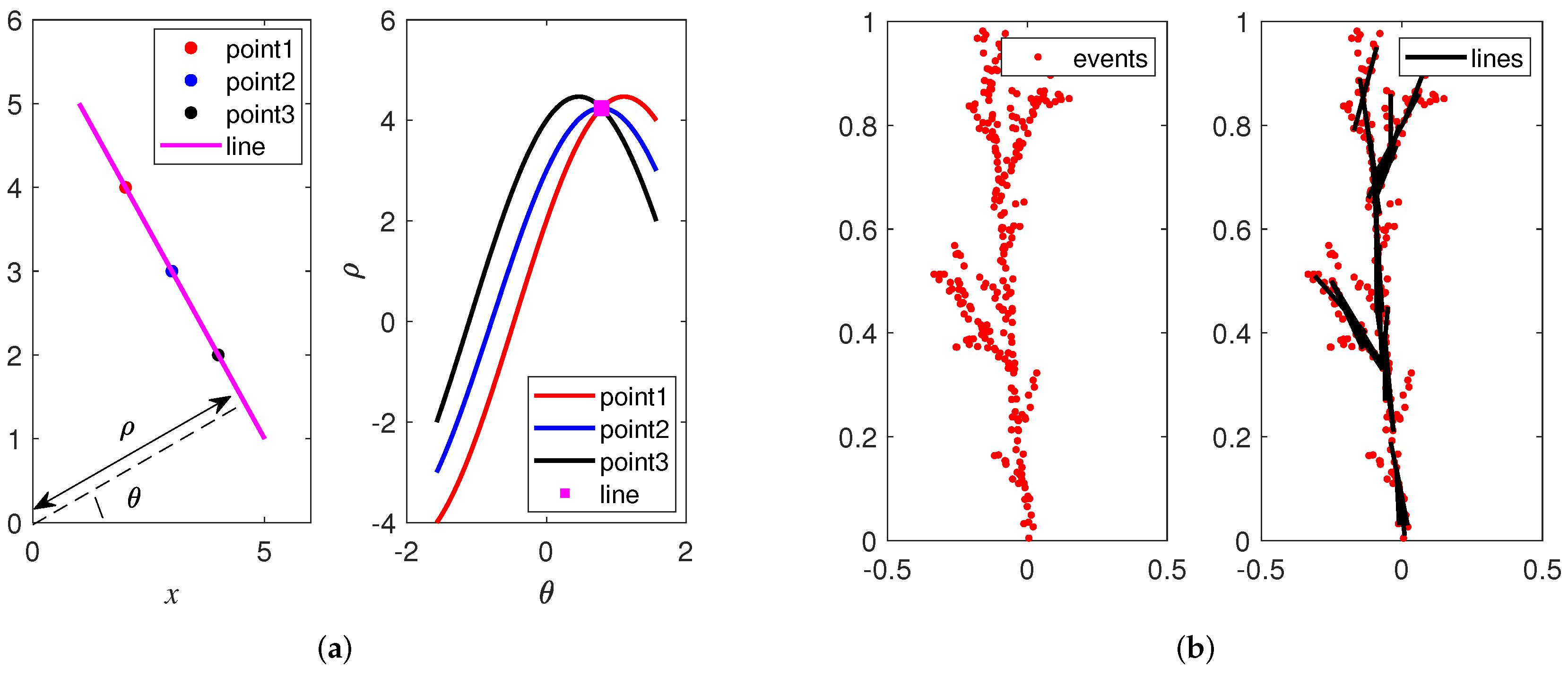
2.2. HF Transform

The Hough transform is an effective method for converting between points and lines or planes. Initially used to detect linear trajectories formed by particle motion, it is now widely applied to the detection of lines and planes in image recognition [24,25,26]. With the help of the Hough transform, the set of discrete lines in the microseismic point cloud can be identified, thus constructing the morphology of the discrete fracture network in the fracture-modified interval marked by microseismic events.

A line in the $x-y$ space can be expressed as $y=kx+b$, which is determined by the value of parameter pair $(k,b)$. Searching for a proper line in the original $x-y$ space can be replaced by some certain optimization problem in the $k-b$ parameter space. Furthermore, the Hough space can be defined as the set of $(\rho ,\theta )$, where $\rho$ represents the distance from the origin to the line, and $\theta$ represents the deflection angle of the normal line. By defining the following accumulator (1), the proper line in the original point cloud can be determined after space discretization and maximum searching, as shown in Figure 1.

$$\begin{array}{c}\hfill A(\rho ,\theta )={\int }_{-\infty }^{\infty }{\int }_{-\infty }^{\infty }I(x,y)\delta (\rho -xcos\theta -ysin\theta )dxdy.\end{array}$$

(1)

Lu and Zhang [27] applied the Hough transform to parameterize discrete fractures, and then used the automatic history matching technique to globally invert the geometric distribution parameters and permeability of two-dimensional discrete fractures. Yu et al. introduced the probabilistic Hough transform to identify important fracture planes in a three-dimensional point cloud, thus constructing a three-dimensional discrete fracture network [28].

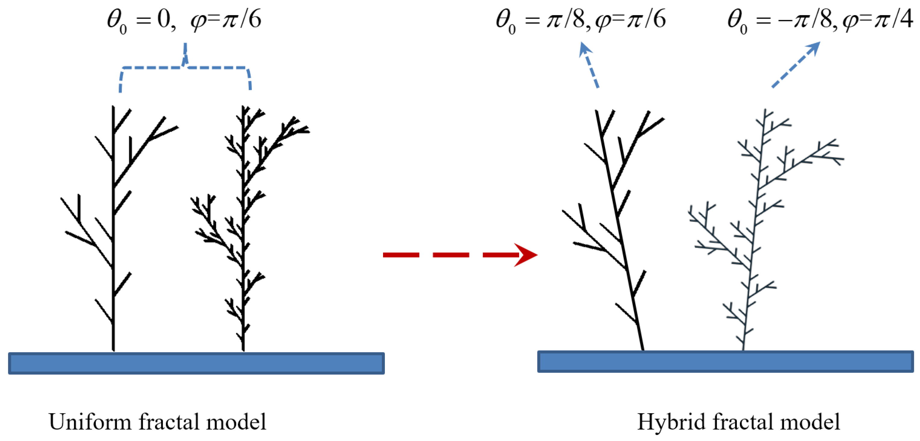
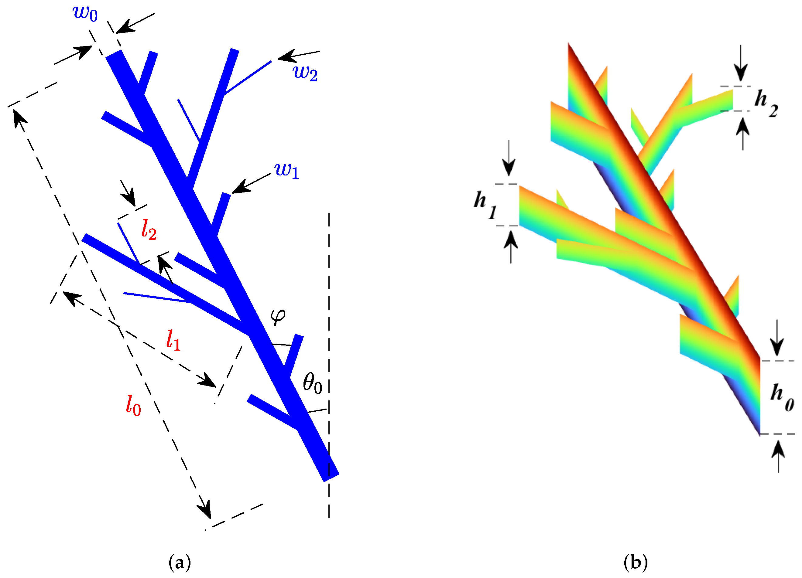
2.3. Fractal Tree

Some studies have shown that the complex fracture network formed during hydraulic fracturing is not chaotic, but exhibits high self-similarity characteristics [29]. Fractal theory is widely used to describe the similarity or self-similarity patterns of objects at different scales [30], and fractal networks have also become one of the main methods for characterizing fractures [21,31,32].

Liu et al. [21] proposed a fractal model that generates a power-law distribution of rock fracture networks using the Monte Carlo method, and uses two fractal dimensions to correlate the fractal characteristics and equivalent permeability of the fracture network. Miao et al. [32] proposed a fractal scaling law for rock fracture length based on fractal theory, and its relationship with fracture area porosity and the ratio of maximum to minimum fracture length. Based on this, a fracture fractal model considering multiple parameters was established. Zhang et al. [16] matched microseismic points based on the fractal L-system, and fitted history production data through the SPSA algorithm to predict fracture parameters. Figure 2 shows three fractal trees with different levels.

2.4. Inversion Problem and Regularization

Directly inferring and calculating the structural parameters of complex fracture networks from certain observation data is not a good choice. A more effective approach is to establish an inversion model through an observation equation. Taking fracture inversion based on microseismic observation data as an example, since the microseisms formed by hydraulic fracturing are multi-sourced, the spatial distribution range is generally small (on the order of hundreds of meters), and the positions of geophones are also spatially limited. This makes the problem not only highly nonlinear but also subject to significant noise interference [33]. Therefore, effective nonlinear inversion methods are necessary for fracture prediction.

Let us denote the observation equation as $G\left(\mathbf{X}\right)=d$, where $\mathbf{X}$ represents the fracture parameters and d is the microseismic observation data. Due to the strong nonlinearity and observation errors mentioned above, this problem is often ill-posed and some regularization techniques are necessary to achieve an effective solution.

Tikhonov regularization is the most commonly used regularization method for solving ill-posed inverse problems, laying a good theoretical foundation for regularization research into inverse problems. The Tikhonov regularization for the above problem can be formulated in the following optimization problem:

$$\begin{array}{c}\hfill \underset{\mathbf{X}}{min}\left|\right|G\left(\mathbf{X}\right)-{d\left|\right|}_2^2+{\alpha \left|\right|D\mathbf{X}\left|\right|}_2^2\end{array}$$

(2)

where the first term is the data fitting term; the second term is the Tikhonov regularization term; and $\alpha$ is the regularization parameter, a constant used to balance the weights of the data fitting term and the regularization term. D represents the differential (or difference) operator, for which the proper order can be set according to different practical problems.

To overcome the over-smoothing shortcoming of Tikhonov regularization, Rudin et al. [34] proposed the use of the relaxed form of the $L_0$ norm, that is, the TV regularization method based on the $L_1$ norm. The TV regularization for the above problem can be expressed in the following optimization form:

$$\begin{array}{c}\hfill \underset{\mathbf{X}}{min}\left|\right|G\left(\mathbf{X}\right)-{d\left|\right|}_2^2+{\alpha \left|\right|D\mathbf{X}\left|\right|}_1\end{array}$$

(3)

The second term is the TV regularization term, which means a convex approximation of the $L_0$ norm. The introduction of the TV regularization term can better ensure the sparsity of the solution, but it has more stringent requirements for the regularization parameter and the numerical algorithm.

3. Proposed Method

Due to the complex flow of oil and gas in fractures, different observation data can only reflect a limited portion of the characteristics of the fractures. It is difficult for a single observation data source, e.g., microseismic, logging, production, etc., to fully reflect the complex fracture network characteristics formed. Therefore, integrating multiple observation data sources for the inversion of complex fracture networks is a natural choice and the basic guarantee for subsequent production optimization. In view of the characteristics of fracture development, this paper introduces a multi-parameter hybrid version for fractal networks, and then formulates a regularization inversion problem based on microseismic data and production data. An optimization algorithm is developed based on an alternating iterative scheme to solve the problem, finally the geometric parameters of complex underground fracture networks are effectively estimated and predicted.

3.1. Hybrid Fractal Model with Multiple Parameters

Parameterized modeling is necessary foundation work before inverting the underground fracture network. However, most of the previous methods assume that fractures on the same fractal scale are determined by the same geometric parameters (width, height, branching angle, etc.). In fact, due to various factors such as geological structure, reservoir characteristics, and fracturing configuration, differences and variations can be found in the geometric parameters of fractures though they are at the same fractal scale. In view of this, we introduce variation in the height and its randomness, and present a hybrid fractal model with multiple parameters.

In this paper, we first construct a basic tree fractal model based an iterative function system (IFS), which is denoted as follows:

$$\begin{array}{c}\hfill \begin{array}{c}{L}_0\left(\begin{array}{c}x\\ y\end{array}\right)=\left(\begin{array}{cc}1/3& 0\\ 0& 1/3\end{array}\right)\left(\begin{array}{c}x\\ y\end{array}\right),L_1\left(\begin{array}{c}x\\ y\end{array}\right)=L_0\left(\begin{array}{c}x\\ y\end{array}\right)+\left(\begin{array}{c}0\\ 1/3\end{array}\right),L_2\left(\begin{array}{c}x\\ y\end{array}\right)=L_0\left(\begin{array}{c}x\\ y\end{array}\right)+\left(\begin{array}{c}0\\ 2/3\end{array}\right),\hfill \\ L_3\left(\begin{array}{c}x\\ y\end{array}\right)=\left(\begin{array}{cc}cos\phi & -sin\phi \\ sin\phi & cos\phi \end{array}\right)L_0\left(\begin{array}{c}x\\ y\end{array}\right)+L_0\left(\begin{array}{c}x\\ y\end{array}\right),L_4\left(\begin{array}{c}x\\ y\end{array}\right)=\left(\begin{array}{cc}cos\phi & sin\phi \\ -sin\phi & cos\phi \end{array}\right)L_0\left(\begin{array}{c}x\\ y\end{array}\right)+L_1\left(\begin{array}{c}x\\ y\end{array}\right).\hfill \end{array}\end{array}$$

(4)

Figure 3 shows one iteration of the above system.

The multi-parameter hybrid fractal network model proposed in this paper is composed of a series of such branching structures. However, unlike the traditional tree fractal network model, this model does not require cracks of the same level to have the same characteristics (height, orientation, branch angle, etc), but adopts a hierarchical adaptive approach to make it more in line with the actual situation. As shown in Figure 4, the left fractal network model is uniform in the orientation ${\theta }_0$ and branch angle $\phi$, while the right one varies these factors.

As shown in Figure 5a, the multi-parameter mixed fractal network model is formed from the initial crack, with a length of $l_0$, a width of $w_0$, and a development direction of ${\theta }_0$. The multi-parameter hybrid fractal network is developed based on a ‘Y’-shaped structure with a branching angle of $\phi$, and the change factors of length and width at the next level relative to the previous level are denoted by ${\alpha }_l$ and ${\alpha }_w$, respectively; that is,

$$\begin{array}{c}\hfill {\alpha }_l={\displaystyle \frac{l_{j+1}}{l_j}},{\alpha }_w={\displaystyle \frac{w_{j+1}}{w_j}},j=0,1,2,\cdots ,n\end{array}$$

(5)

where $l_j$ and $w_j$ mean the length and width of the fracture at level j.

The height of fracturing fractures is influenced by various complex factors, including geological structure, reservoir characteristics, and fracturing construction parameters. These factors lead to irregular changes in height. The traditional tree fractal network model assumes a uniform height at the same level; however, there should also be subtle differences and variations in the height of cracks at the same level. Therefore, the multi-parameter hybrid fractal network model considers the height of cracks at the same level as a Gaussian distribution with a mean of $h_j$, as shown in Figure 5b. And the mean height at the next level is proportional to that at the previous level; that is,

$$\begin{array}{c}\hfill p\left(h\right)={\displaystyle \frac{1}{\sqrt{2\pi }\sigma }}exp(-{\displaystyle \frac{{(h-h_j)}^2}{2{\sigma }^2}}),h_{j+1}={\alpha }_h{h}_j,j=0,1,2,\cdots ,n\end{array}$$

(6)

where ${\alpha }_h$ denotes the change factor of the mean of the fracture height, and $\sigma$ denotes the standard variance.

In summary, the multi-parameter hybrid fractal network can be modeled as the following characterization parameters after the root positions and level number are preset.

(1)

Initial length $l_0$, width $w_0$, height mean $h_0$, standard variance $\sigma$, and development direction ${\theta }_0$;

(2)

Change factors ${\alpha }_l,{\alpha }_w$, and ${\alpha }_h$;

(3)

Branching angle $\phi$.

For convenience of discussion, it is natural to introduce the vector $\mathbf{X}=$$[l_0,w_0,h_0,\sigma ,{\theta }_0,\phi ,{\alpha }_l,{\alpha }_w,{\alpha }_h]$.

3.2. A Joint Regularization Model for Inverse Fracture Parameters

When performing hydraulic fracturing or high-pressure water injection operations on site, the pressure of the surrounding strata around the wellbore will gradually increase. This pressure change will cause internal defects in the formation rock to be compressed and crack, while releasing low-energy sound waves, known as microseismic events [16]. This series of reactions ultimately leads to the formation of hydraulic fracturing fractures. Based on the mathematical model of seismic wave propagation, the three-dimensional spatial position of the seismic source can be obtained, and the geometric parameters of the fracturing fracture can be further derived.

The source coordinates can not only be used to calculate the geometric parameters of hydraulic fracturing fractures, but also to simulate the specific morphology of fractures formed during hydraulic fracturing construction [12,32]. This usually relies on specific crack characterization models, such as discrete crack network models and tree fractal network models. Then, by adjusting the control parameters of the characterization model, the source coordinates are fitted. Taking the fractal fracture model as an example, each node in the fractal network can be matched with the seismic source position. By minimizing the total distance error between all fractal nodes and the seismic source position, simulation of the specific morphology of fracturing fractures can be achieved:

$$\begin{array}{c}\hfill \underset{\mathbf{X}}{min}\sum _{i=1}^M\underset{j}{min}{[nod{e}_j\left(\mathbf{X}\right)-sourc{e}_i]}^2\end{array}$$

(7)

where $nod{e}_j\left(\mathbf{X}\right)$ denotes the position node j in the fractal network determined by the parameter $\mathbf{X}$, and $sourc{e}_i$ means the position of detected seismic source i. The objective function calculates the proximity between the spatial location of the seismic source and the crack network, as shown in Figure 6a. Optimizing the objective function can drive the parametric vector $\mathbf{X}$ to evolve to a proper situation where the fracture network holds with a suitable geometric shape and explains the seismic events well.

The parameters of the fracture network have a crucial impact on the seepage process of underground gas reservoirs. Therefore, the transfusion characteristics in fractures can be estimated based on production data, and then the geometric parameters of the fractures can be determined.

The gas-flowing space in shale reservoirs can be divided into two systems: the matrix and the fractures. Here, we first give some basic equations necessary for discussing the flow in the matrix.

The total gas per unit volume in the matrix can be denoted as

$$\begin{array}{c}\hfill \int \left[\varphi CM+(1-\varphi )C_{\mu }M\right]\end{array}$$

(8)

where C denotes the molar number of free gas per unit pore volume, $\varphi$ is the matrix porosity, $C_{\mu }$ denotes the molecules of adsorbed gas per unit pore volume, and M means the molar mass of gas.

Then, the viscous flow and Knudsen diffusion can be denoted as

$$\begin{array}{c}\hfill \mathbf{J}=-D_k\nabla \left(CM\right)+{\displaystyle \frac{v}{\varphi }}\left(CM\right)\end{array}$$

(9)

where v denotes the Darcy flow velocity of free gas in porous media, and $D_k$ denotes the Knudsen diffusion coefficient.

The diffusion of adsorbed gas on the surface of a solid unit can be expressed as

$$\begin{array}{c}\hfill {\mathbf{J}}_{\mathbf{ad}}=-D_{ad}\nabla \left(C_{\mu }M\right)\end{array}$$

(10)

where $D_{ad}$ denotes the diffusion coefficient of adsorbed gas on the surface of rocks.

Considering a non-equilibrium Langmuir process, and introducing an equivalent permeability mechanism, the gas migration in the matrix system can be formulated as

$$\begin{array}{c}\hfill {\displaystyle \frac{\partial C}{\partial t}}-{\displaystyle \frac{{\kappa }_{a}RT}{\mu \varphi }}\nabla ·(C\nabla C)=-{\displaystyle \frac{1-\varphi }{\varphi }}{R}_{net}\end{array}$$

(11)

where C denotes the molar number of free gas per unit pore volume, $\varphi$ is the matrix porosity, ${\kappa }_a={\kappa }_{mi}(1+{\displaystyle \frac{p_0}{p}}{\displaystyle \frac{1}{\overline{\lambda }}})$ is the equivalent permeability, and $\overline{\lambda }$ is a dimensionless quantity linked to the dominant role of viscous flow and Knudsen diffusion. ${\kappa }_{mi}$ is the original permeability of matrix system. $R_{net}$ is the net adsorption capacity per unit time. For details, refer to [10,35].

And after a similar formal analysis, the gas migration in the fracture system can be formulated as

$$\begin{array}{c}\hfill {\varphi }_f{\displaystyle \frac{\partial C_f}{\partial t}}+{\displaystyle \frac{\partial }{\partial x}}\left(C_f{u}_f\right)+{\displaystyle \frac{\partial }{\partial z}}\left(C_f{w}_f\right)+(1-{\varphi }_f){\displaystyle \frac{\partial C_{\mu f}}{\partial t}}=0\end{array}$$

(12)

where $C_f$ denotes the molar number of free gas per unit fracture volume. $u_f$ and $w_f$ denote the permeability velocities along the x-axis and z-axis, and they are determined by the fracture network, more exactly, the parametric vector $\mathbf{X}$. $C_{\mu f}$ denotes the adsorbed gas concentration and ${\varphi }_f$ denotes the fracture porosity. $C_{\mu f}$ denotes the adsorbed gas concentration in the fractures.

As the fracture parameters of X are fixed and proper initial boundary conditions given, the gas flow in the matrix fracture system can be solved numerically. For convenience of discussion, we formulated the gas production calculated based on the numerical gas flow as $prod(t,\mathbf{X})$. Then, the fracture parameters can be optimized by minimizing the fitting error of gas production:

$$\begin{array}{c}\hfill \underset{\mathbf{X}}{min}\sum _t{[prod(t,\mathbf{X})-production\left(t\right)]}^2\end{array}$$

(13)

where $production\left(t\right)$ means the production data at time t. A similar PDE-based optimization can be found in some related works [36,37,38].

Based on models (7) and (13), we can directly obtain a joint inversion model for fracture parameters:

$$\begin{array}{c}\hfill \underset{\mathbf{X}}{min}\sum _{i=1}^M\underset{j}{min}{[nod{e}_j\left(\mathbf{X}\right)-sourc{e}_i]}^2+\sum _t{[prod(t,\mathbf{X})-production\left(t\right)]}^2.\end{array}$$

(14)

However, it is difficult to solve such a strong nonlinear and nonconvex problem. It is natural to introduce regularization techniques and the novel joint regularization model can be denoted as

$$\begin{array}{c}\hfill \underset{\mathbf{X}}{min}{\left|\right|\mathbf{X}\left|\right|}_2^2+{\lambda }_1\sum _i^M\underset{j}{min}{[nod{e}_j\left(\mathbf{X}\right)-sourc{e}_i]}^2+{\lambda }_2\sum _t{[prod(t,\mathbf{X})-production\left(t\right)]}^2.\end{array}$$

(15)

Because the microseismic data are more closely related to the fracture location parameters while the production data are more closely related to the fracture flow capacity parameters, it is advantageous to split the variable X into two parts, that is, ${\mathbf{X}}_1$ and ${\mathbf{X}}_2$, and the model (16) can be rewritten as

$$\begin{array}{}\mathrm{(16)}& \hfill \underset{{\mathbf{X}}_1,{\mathbf{X}}_2}{min}E\left(\mathbf{X}\right)=& E_1\left([{\mathbf{X}}_1,{\mathbf{X}}_2]\right)+E_2\left([{\mathbf{X}}_1,{\mathbf{X}}_2]\right)\hfill \mathrm{(17)}& \hfill =& \left|\right|{\mathbf{X}}_1{\left|\right|}_2^2+{\lambda }_1\sum _{i=1}^M\underset{j}{min}{[nod{e}_j\left([{\mathbf{X}}_1,{\mathbf{X}}_2]\right)-sourc{e}_i]}^2\hfill \mathrm{(18)}& & +\left|\right|{\mathbf{X}}_2{\left|\right|}_2^2+{\lambda }_2\sum _t{[prod(t,[{\mathbf{X}}_1,{\mathbf{X}}_2])-production\left(t\right)]}^2.\hfill \end{array}$$

Here, $\mathbf{X}=[l_0,w_0,h_0,\sigma ,{\theta }_0,\phi ,{\alpha }_l,{\alpha }_w,{\alpha }_h]$, ${\mathbf{X}}_1=[l_0,h_0,\sigma ,{\theta }_0,\phi ]$ means the fracture geometric parameter vector while $X_2=[w_0,{\alpha }_l,{\alpha }_w,{\alpha }_h]$ means the fracture flow capacity parameter vector.

Based on the variational method and gradient descent, an alternative iterative algorithm (Algorithm 1) is proposed to solve the joint regularization model above.

Algorithm 1 Alternative Iterative Inversion Algorithm

Require:  Initial $X_1^{\left(0\right)}$, $X_2^{\left(0\right)}$, ${\lambda }_1$, ${\lambda }_2$, $\epsilon$, $maxIter$. Ensure:  Optimal solution $X_1,X_2$   1: $j=0$;   2: while $\left|\right|\Delta E\left|\right|>\epsilon$ and $j<maxIter$ do   3:     $i=0,X_1^{\left(i\right)}=X_1^{\left(j\right)}$;   4:     while $\left|\right|\Delta E_1\left|\right|>\epsilon$ and $i<maxIter$ do   5:         $\Delta E_1={\displaystyle \frac{\partial }{\partial X_1}}{E}_1\left([X_1^{\left(i\right)},X_2^{\left(j\right)}]\right)$;   6:         $X_1^{(i+1)}=X_1^{\left(i\right)}-\Delta E_1$;   7:     end while   8:     $X_1^{(j+1)}=X_1^{\left(i\right)}$   9:     $i=0,X_2^{\left(i\right)}=X_2^{\left(j\right)}$; 10:     while $\left|\right|\Delta E_2\left|\right|>\epsilon$ and $i<maxIter$ do 11:         $\Delta E_2={\displaystyle \frac{\partial }{\partial X_2}}{E}_2\left([X_1^{\left(j\right)},X_2^{\left(i\right)}]\right)$; 12:         $X_1^{(i+1)}=X_1^{\left(i\right)}-\Delta E_1$; 13:     end while 14:     $X_2^{(j+1)}=X_2^{\left(i\right)},j=j+1$; 15:     $\Delta E=\Delta E_1+\Delta E_2$; 16: end while 17: $X_1=X_1^{\left(j\right)},X_2=X_2^{\left(j\right)}$.

4. Experiments and Results

In this section, we arrange several experiments to illustrate the performance and advantages of the proposed method.

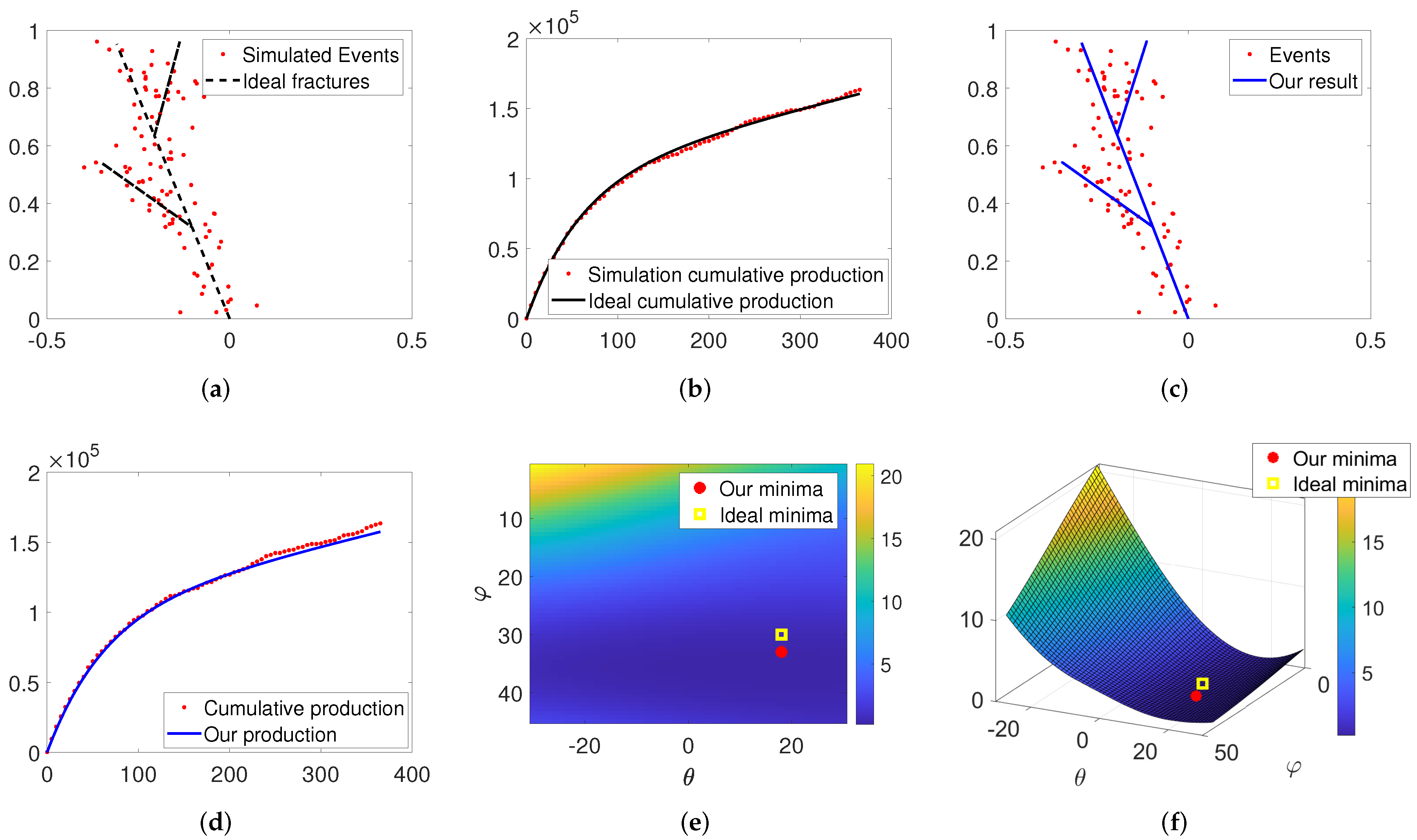
4.1. Synthetic Test 1

In the first experiment, we simulate a simple fractal tree as an ideal fracture for testing. In order to reflect the actual scene as realistically as possible, certain noise is added to simulate the real situation. The 100 red points shown in Figure 7a represent the seismic events around the ideal fractures, which are marked as dashed lines.

For a convenient test, we also simulate 365 production data based on the ideal fracture, as shown in Figure 7b. The corresponding actual scenario is the initial stage of production, where the output rapidly increases and gradually stabilizes.

Some related parameters applied in the simulation are shown in

Table 1. Values of parameters in simulation.

Symbol	Meaning	Value	Symbol	Meaning	Value
$\varphi$	Matrix porosity	0.02	${\varphi }_f$	Fracture porosity	0.2
${\kappa }_{mi}$	Original matrix permeability	100 nD	$D_k$	Knudsen coefficient	$1\times {10}^{-3}{\mathrm{cm}}^2/\mathrm{s}$
$D_{ad}$	Adsorbed gas coefficient	$1\times {10}^{-5}{\mathrm{cm}}^2/\mathrm{s}$	M	Molar mass of gas	16.043 g/mol
R	Pore radius	40 nm	$p_0$	Original Reservoir pressure	20 Mpa
T	Reservoir Temperature	300 K	$w_0$	Fracture initial width	5 mm

.

The solved fracture and production are shown in Figure 7c,d. Error surfaces projected in the parameter space $\theta -\phi$ are shown in the last two subfigures.

It can be found that the inversion result of the parameters well represents the fracture position and geometric structure. The error surfaces in Figure 7e,f show a slight difference between our result and the ideal minimum point. The relative error of the minimal value can be found to be about 4.94%. The parameter $\theta =\pi /10$ can be solved accurately, while an absolute error of $\pi /90$ is found for the parameter $\phi =pi/6$.

4.2. Synthetic Test 2

For a further test, we simulate a relative complex fractal tree as ideal fractures in this experiment. Figure 8a shows the ideal fracture (in dashed lines) and the simulated 500 seismic events (marked by red points). There are 365 production data based on the ideal fracture, as shown in Figure 8b. The solved fracture and the related history match are shown in Figure 8c,d. Error surfaces projected in the parameter space $\theta -\phi$ are shown in Figure 8e,f.

It can be also found that the inversion result of the fracture parameters represents the geometric structure well, as shown in Figure 8c. The history match can be also well achieved based on the fracture inversion, as shown in Figure 8d. From the error surfaces shown in Figure 8e,f, just a little more difference between our result and the ideal minimum point can be found than in synthetic test 1. In more detail, the relative error of the minimal value can be found to be about 6.48%. Absolute errors of $\pi /180$ and $\pi /36$ can be found, respectively, in solving the parameters $\theta =\pi /9$ and $\phi =pi/6$. This means that the more complex the fracture structure is, the more difficult accurate computation is.

It seems the proposed method achieved satisfactory results and success in solving the inversion problem. However, though we have tried to simulate the actual scene as realistically as possible, there are still many differences between the simulated data and real data, so more tests related to real data should be introduced to fully validate the accuracy and efficiency of our method.

4.3. Test on Real Data

For a more convincing test, we collected some real seismic data (in 30 stages) and 345 production data (from 16 November 2018 to 26 October 2019) of a shale gas well (named Well X), as partially shown in

Table 2. Microseismic data.

Stage	Number of Events	Length	Width	Height	Orientation
Stage 1	68	350	85	65	85
Stage 2	114	200	50	40	90
Stage 3	69	330	90	90	75
Stage 4	72	180	100	80	85
Stage 5	116	180	100	75	90
…	…	…	…	…	…
Stage 29	50	145	108	38	114
Stage 30	39	180	89	67	91

and

Table 3. Production data.

Well	Day Index	Date	Production Hours	Daily Gas	Cumulative Gas
Well X	1	16 November 2018	24	6.4994	6.50
Well X	2	17 November 2018	24	10.7639	17.26
Well X	3	18 November 2018	24	14.1072	31.37
Well X	4	19 November 2018	24	21.0404	52.41
…	…	…	…	…	…
Well X	344	25 October 2019	24	8.2233	6193.89
Well X	345	26 October 2019	24	2.2443	6196.13

. A scatter plot of the seismic events and the cumulative production curve are shown in Figure 9a,b.

After applying the proposed model (16) and Algorithm 1, the geometrical parameters X can be solved efficiently and then the final fractures can be determined as shown in Figure 9c.

The geometric match between the solved fractures and the observed seismic events is shown in Figure 9d. It can be found that our inversion result represents the event region well (and the geometric properties, such as length, width, area, etc.) in each stage. The history match of the production are shown in Figure 9e and the mean square relative error is no more than 7.73%.

5. Discussion and Conclusions

In this paper, a joint regularization model is introduced to invert the fracture geometric parameters with the microseismic observation and production data. Based on fractal theory and a hybrid strategy, the fracture network can be modeled in a more flexible pattern to treat more complex situations. Then, different energy functionals are introduced to describe the error between the observation data and the multi-parameter fractal model. Regularization terms are joined to address the ill-posedness, then the proposed model can be solved by an alternative iterative algorithm. Three experiments are arranged to validate the advantage of the proposed joint regularization model. The experimental results based on synthetic data and real data show the accuracy and efficiency of the proposed method.

5.1. Limitations

The proposed method has achieved certain results, but there are still some limitations.

(1) This paper develops fracture and flow modeling based on certain assumptions, which simplify complex practical situations and may affect the accuracy of the inversion results and their applicability in complex shale reservoirs. (2) This paper did not investigate the impact of data quality and data characteristics on the inversion results. Different shale gas wells may have significant differences in data quality or data characteristics, and the effectiveness of the method proposed in this paper still needs to be verified. (3) This paper did not investigate the impact of different regularization techniques on its method, and the applicability of the regularization techniques used for the inversion problem in this article also needs to be verified in more situations or more analytical conclusions need to be sought to support it.

5.2. Future Work

In addition to improving on the limitations mentioned above, this study may be further developed in the following three aspects in the future.

(1) Microseismic observation data and production data can provide crack observation information from two dimensions. If more observation dimensions can be expanded to enrich crack observation information, then more flexible joint inversion approaches can be used.

(2) Introducing more advanced optimization techniques to more effectively solve the inversion problem of fracture parameters under a set of given observations can further enhance the application potential of the method.

(3) Further comprehensive mechanism modeling, and multimodal and multi-field coupling can be used to establish new inversion models, improving the inversion performance and application prospects.

References

- Bowker, K.A. Barnett Shale gas production, Fort Worth Basin: Issues and discussion. AAPG Bull. 2007, 91, 523–533. [Google Scholar] [CrossRef]
- Zou, C.; Zhao, Q.; Dong, D.; Yang, Z.; Qiu, Z.; Liang, F.; Wang, N.; Huang, Y.; Duan, A.; Zhang, Q.; et al. Geological characteristics, main challenges and future prospect of shale gas. J. Nat. Gas Geosci. 2017, 2, 273–288. [Google Scholar]
- Mayerhofer, M.J.; Lolon, E.P.; Youngblood, J.E.; Heinze, J.R. Integration of microseismic fracture mapping results with numerical fracture network production modeling in the Barnett shale. In Proceedings of the SPE Annual Technical Conference and Exhibition, San Antonio, TX, USA, 24–27 September 2006; p. SPE-102103. [Google Scholar]
- Li, Q.; Li, Q.; Cao, H.; Wu, J.; Wang, F.; Wang, Y. The Crack Propagation Behaviour of CO2 Fracturing Fluid in Unconventional Low Permeability Reservoirs: Factor Analysis and Mechanism Revelation. Processes 2025, 13, 159. [Google Scholar] [CrossRef]
- Zang, C.; Jiang, H.; Shi, S.; Li, J.; Zou, Y.; Zhang, S.; Tian, G.; Yang, P. An analysis of the uniformity of multi-fracture initiation based on downhole video imaging technology: A case study of Mahu tight conglomerate in Junggar Basin, NW China. Pet. Explor. Dev. 2022, 49, 448–457. [Google Scholar] [CrossRef]
- Hou, B.; Chen, M.; Li, Z.; Wang, Y.; Diao, C. Propagation area evaluation of hydraulic fracture networks in shale gas reservoirs. Pet. Explor. Dev. 2014, 41, 833–838. [Google Scholar]
- Li, Y.; Liu, D.; Zhai, Y.; Shi, W.; Xian, Y. 3-D FEM azimuth forward modeling of hydraulic fractures based on electromagnetic theory. IEEE Geosci. Remote Sens. Lett. 2020, 18, 246–250. [Google Scholar]
- Chen, M.; Guo, T.; Xu, Y.; Qu, Z.; Zhang, S.; Zhou, T.; Wang, Y. Evolution mechanism of optical fiber strain induced by multi-fracture growth during fracturing in horizontal wells. Pet. Explor. Dev. 2022, 49, 211–222. [Google Scholar]
- Zhao, J.; Li, Y.; Wang, S.; Jiang, Y.; Zhang, L. Simulation of complex fracture networks influenced by natural fractures in shale gas reservoir. Nat. Gas Ind. B 2014, 1, 89–95. [Google Scholar]
- Doe, T.; Lacazette, A.; Dershowitz, W.; Knitter, C. Evaluating the effect of natural fractures on production from hydraulically fractured wells using discrete fracture network models. In Proceedings of the SPE/AAPG/SEG Unconventional Resources Technology Conference, URTEC, Denver, CO, USA, 12–14 August 2013; p. URTEC-1581931. [Google Scholar]
- Zhu, H.; Yang, X.; Liao, R.; Gao, D. Microseismic fracture interpretation and application based on parameters inversion. Geophys. Prospect. Pet. 2017, 56, 150–157. [Google Scholar]
- Rudzinski, L.; Debski, W. Extending the double difference location technique—Improving hypocenter depth determination. J. Seismol. 2013, 17, 83–94. [Google Scholar]
- Mi, L. Inversion method of discrete fracture network of shale gas based on gas production profile. Acta Pet. Sin. 2021, 42, 481. [Google Scholar]
- Clarkson, C.; Williams-Kovacs, J. A new method for modeling multi-phase flowback of multi-fractured horizontal tight oil wells to determine hydraulic fracture properties. In Proceedings of the SPE Annual Technical Conference and Exhibition? New Orleans, LA, USA, 30 September–2 October 2013; p. D031S041R007. [Google Scholar]
- Dai, C.; Liu, H.; Wang, Y.; Li, X.; Wang, W. A simulation approach for shale gas development in China with embedded discrete fracture modeling. Mar. Pet. Geol. 2019, 100, 519–529. [Google Scholar] [CrossRef]
- Zhang, K.; Ma, X.; Li, Y.; Wu, H.; Cui, C.; Zhang, X.; Zhang, H.; Yao, J. Parameter prediction of hydraulic fracture for tight reservoir based on micro-seismic and history matching. Fractals 2018, 26, 1840009. [Google Scholar] [CrossRef]
- Zhang, L.; He, X.; Li, X.; Li, K.; He, J.; Zhang, Z.; Guo, J.; Chen, Y.; Liu, W. Shale gas exploration and development in the Sichuan Basin: Progress, challenge and countermeasures. Nat. Gas Ind. B 2022, 9, 176–186. [Google Scholar] [CrossRef]
- Fisher, M.; Heinze, J.; Harris, C.; Davidson, B.; Wright, C.; Dunn, K. Optimizing horizontal completion techniques in the Barnett shale using microseismic fracture mapping. In Proceedings of the SPE Annual Technical Conference and Exhibition, Houston, TX, USA, 26–29 September 2004; p. SPE-90051. [Google Scholar]
- Bian, H.L.; Guan, J.; Mao, Z.Q.; Ju, X.D.; Han, G.Q. Pore structure effect on reservoir electrical properties and well logging evaluation. Appl. Geophys. 2014, 11, 374–383. [Google Scholar] [CrossRef]
- Sun, Z.; Yang, S.; Zhang, F.; Lu, J.; Wang, R.; Ou, X.; Lei, A.; Han, F.; Cen, W.; Wei, D.; et al. A reconstructed method of acoustic logging data and its application in seismic lithological inversion for uranium reservoir. Remote Sens. 2023, 15, 1260. [Google Scholar] [CrossRef]
- Liu, R.; Jiang, Y.; Li, B.; Wang, X. A fractal model for characterizing fluid flow in fractured rock masses based on randomly distributed rock fracture networks. Comput. Geotech. 2015, 65, 45–55. [Google Scholar] [CrossRef]
- Wan, T.; Sheng, J.; Soliman, M.; Zhang, Y. Effect of fracture characteristics on behavior of fractured shale-oil reservoirs by cyclic gas injection. SPE Reserv. Eval. Eng. 2016, 19, 350–355. [Google Scholar] [CrossRef]
- Li, Q.; Li, Q.; Wu, J.; Li, X.; Li, H.; Cheng, Y. Wellhead stability during development process of hydrate reservoir in the Northern South China Sea: Evolution and mechanism. Processes 2024, 13, 40. [Google Scholar] [CrossRef]
- Hough, P.V. Method and Means for Recognizing Complex Patterns. U.S. Patent 3,069,654, 18 December 1962. [Google Scholar]
- Duda, R.O.; Hart, P.E. Use of the Hough transformation to detect lines and curves in pictures. Commun. ACM 1972, 15, 11–15. [Google Scholar] [CrossRef]
- Bhattacharya, P.; Rosenfeld, A.; Weiss, I. Point-to-line mappings as Hough transforms. Pattern Recognit. Lett. 2002, 23, 1705–1710. [Google Scholar]
- Lu, L.; Zhang, D. Assisted history matching for fractured reservoirs by use of hough-transform-based parameterization. SPE J. 2015, 20, 942–961. [Google Scholar]
- Yu, X.; Rutledge, J.; Leaney, S.; Maxwell, S. Discrete-fracture-network generation from microseismic data by use of moment-tensor-and event-location-constrained hough transforms. SPE J. 2016, 21, 221–232. [Google Scholar]
- Barton, C.C.; La Pointe, P.R. Fractals in Petroleum Geology and Earth Processes; Springer Science & Business Media: Berlin/Heidelberg, Germany, 2012. [Google Scholar]
- Zhao, Y.; Wang, C.; Ning, L.; Zhao, H.; Bi, J. Pore and fracture development in coal under stress conditions based on nuclear magnetic resonance and fractal theory. Fuel 2022, 309, 122112. [Google Scholar]
- Liu, R.; Li, B.; Jiang, Y. A fractal model based on a new governing equation of fluid flow in fractures for characterizing hydraulic properties of rock fracture networks. Comput. Geotech. 2016, 75, 57–68. [Google Scholar] [CrossRef]
- Miao, T.; Yu, B.; Duan, Y.; Fang, Q. A fractal analysis of permeability for fractured rocks. Int. J. Heat Mass Transf. 2015, 81, 75–80. [Google Scholar] [CrossRef]
- Kummerow, J. Using the value of the crosscorrelation coefficient to locate microseismic events. Geophysics 2010, 75, MA47–MA52. [Google Scholar]
- Rudin, L.I.; Osher, S.; Fatemi, E. Nonlinear total variation based noise removal algorithms. Phys. D Nonlinear Phenom. 1992, 60, 259–268. [Google Scholar]
- Xia, Y.; Deng, Y.; Wei, S.; Jin, Y. Numerical simulation of multi-scale coupled flow in after-fracturing shale gas reservoirs. Chin. J. Theor. Appl. Mech. 2023, 55, 616–629. [Google Scholar]
- Rees, T.; Dollar, H.S.; Wathen, A.J. Optimal solvers for PDE-constrained optimization. SIAM J. Sci. Comput. 2010, 32, 271–298. [Google Scholar]
- van Leeuwen, T.; Herrmann, F.J. A penalty method for PDE-constrained optimization in inverse problems. Inverse Probl. 2015, 32, 015007. [Google Scholar] [CrossRef]
- Peng, Y.; Zhou, B.; Qi, F. PDE-Constrained Scale Optimization Selection for Feature Detection in Remote Sensing Image Matching. Mathematics 2024, 12, 1882. [Google Scholar] [CrossRef]