1. Introduction
The exhaust gas temperature (EGT) across the turbine outlet is a critical parameter in internal combustion engines, influencing combustion efficiency, emission conversion efficiency, and turbine and after-treatment (AT) integrity and reliability. In the last decades, the automotive sector has been driven by regulations to control with increasing accuracy both the efficiency of the overall energy conversion process (to reduce CO
2 emissions, i.e., brake-specific fuel consumption) and the reliability of the AT system, reducing the emission concentration [
1,
2].
As is well known, the EGT represents a key parameter to be managed in modern engine control, even if it is not directly measured on final production applications [
3]. For this reason, the physical dependence of the EGT on other engine parameters has been widely investigated [
4], such as for different, on-board compatible methods for the estimation of the temperature. Indeed, there are in the literature several works describing the indirect measurement of the exhaust gas temperature with an universal exhaust gas oxygen (UEGO) probe [
5] or methodologies for direct modelling, which can be grouped as follows:
Mean value models for EGT estimation [
6,
7,
8];
Data-driven approaches [
9,
10,
11];
0-D physical and semi-physical methods grounded in thermodynamics and heat transfer equations [
12,
13,
14];
The raw EGT measurement available at the engine test cell is typically performed with thermocouple (TC), and physical or semi-physical models could include the sensor effect for the final temperature estimation [
18]. A TC introduces both a delay in the temperature sensing that has an effect, especially under transient conditions, and an offset with respect to the temperature measured with other sensors [
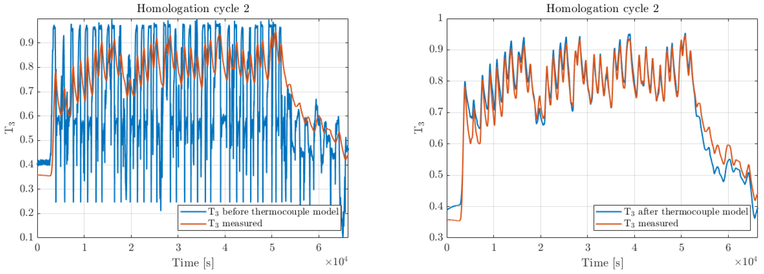
19]. This second aspect is typically not fully considered, since a TC is often used to evaluate the temperature limits too (for example temperature limitation at the turbine inlet in turbocharged engine and gas turbines). This means the TC measurement becomes a reference and the temperature delta between the measurement and the gas temperature can be neglected. On the other hand, the delay introduced by TC dynamics can be well represented by a first-order system, where the time constant τ can be calibrated for the particular features of the used sensor (i.e., the sensing tip size and type of thermocouple).
One of the main limitations of pure data-driven methods is the extrapolation capability, even with important differences between various algorithms [
20,
21]. Generally speaking, machine learning models typically need wide databases for training and they cannot guarantee a high accuracy when inputs assume values outside the range considered for algorithm training [
22]. For both these reasons, authors have already effectively developed and implemented hybrid approaches where a machine learning algorithm is mainly used to include the effect of input features that do not vary outside the range assumed in the training database, while analytical functions are instead used to describe the physical relationship between inputs that could change significantly and the output [
23]. Thus, this hybrid approach can be considered halfway between methods 2 and 3 listed above.
The literature is not so populated in the field of hybrid modeling approaches, and in particular the application of such methods for the estimation of the EGT at the turbine outlet can be considered as a quite innovative contribution in this field. In fact, the majority of recent works that describe data driven-based exhaust gas temperature models [
24,
25] are focused on the procedures for the hyperparameters’ optimization and input features’ selection. The comparison between different machine learning approaches is another widely presented topic, as described in [
26]. On the contrary, the present work deals with the development of a viable strategy to enhance the extrapolation capability of pure data-driven approaches and to extend their applicability to conditions unseen during the training phase. The innovative contribution of the research is thus the simplification of a complicated phenomenon into simpler sub-problems, on the base of the physics of the system, and the application of most appropriate modeling approach to each. The application of a hybrid approach to engine modeling demonstrates that integrated models, which blend analytical functions with artificial neural networks (ANNs), achieve superior predictive accuracy and generalization performance compared to models relying solely on ANNs. This type of modeling approach is based on the effects of superposition principle [
27], and this means each input variable brings a specific contribution to the physical process [
28,
29]. With a hybrid approach, it is possible to improve the accuracy of each method (pure data-driven and pure analytical) when used as the main approach, maintaining a low computational effort for the complete algorithm. Developing models requiring low computational power to be executed is important for deploying them in real-time (RT) devices. Authors typically deal with the development of innovative sensors [
30] and control-oriented engine and combustion models compatible with RT execution and their implementation in RT control strategies [
31]. This objective is maintained also for the EGT modeling activity.
In this work, the aforementioned hybrid approach is applied to model the EGT at the turbine outlet, starting from the estimation of the temperature at the turbine inlet, which serves as an input for modeling the expansion across the turbine impeller. Expansion modeling is approached with equations of the physical process. This study aims to assess the advantages and limitations of this approach in terms of its accuracy and adaptability to varying operational conditions. The results provide valuable insights into the reliability of hybrid models, where ANNs and physical 0-D functions work together to improve the reliability of the overall model in terms of extrapolation capability.
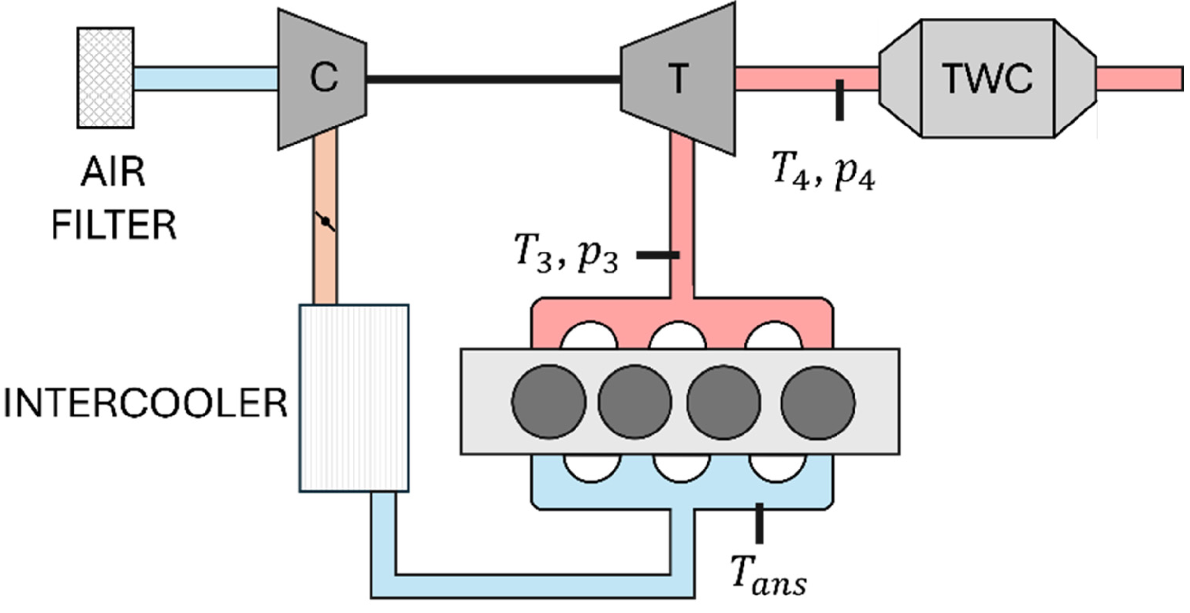
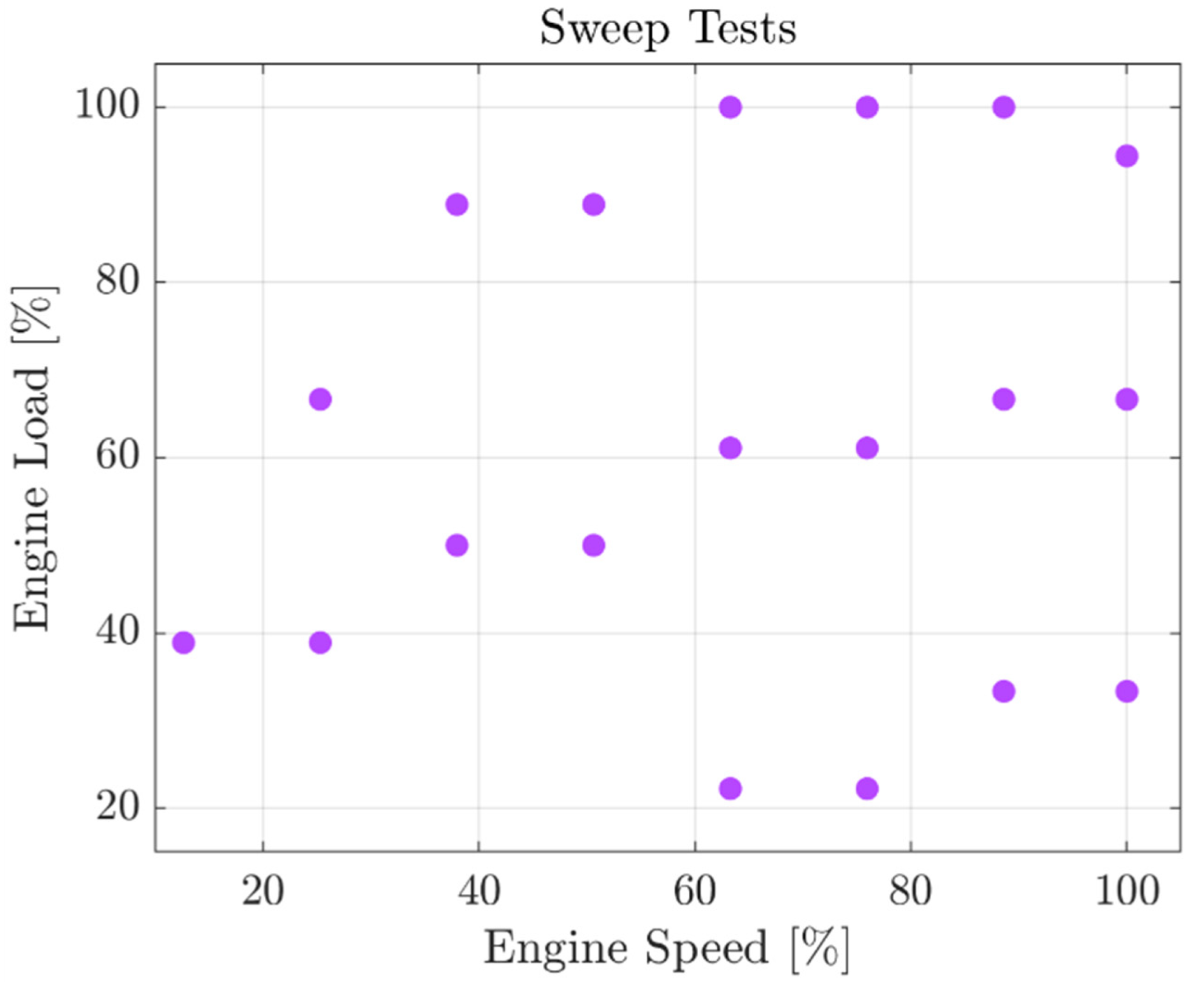
In the first part, the experimental setup used to collect experimental datasets for the model development and validation is presented and the type of tests carried out at the test rig for data collection are described. Both steady states and transient states are recorded, because the model is developed with steady-state data only and validated under transient conditions. The engine is a turbocharged, gasoline direct injection (GDI), V8 engine and the model developed in this work refers to a single engine bank.
The modeling approach is then presented in
Section 3, highlighting the part of the model in which ANNs, analytical functions, and physical equations are implemented. In this section, the complete calculation chain for the estimation of the exhaust gas temperature at the turbine outlet. The EGT before the turbine impeller (
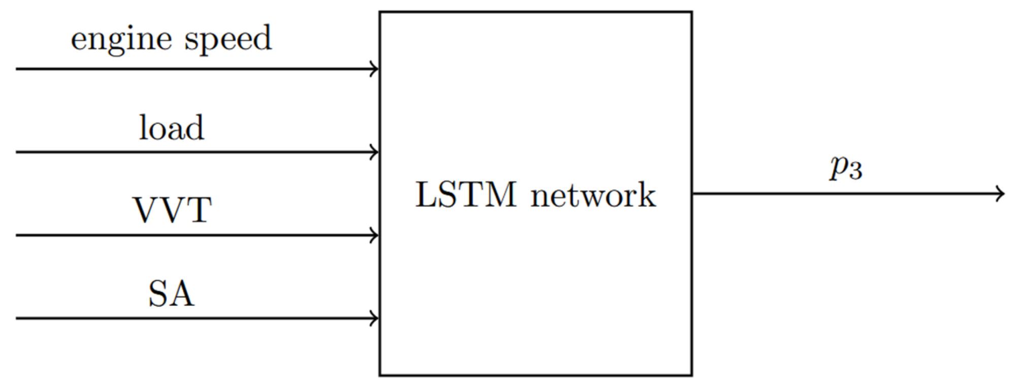
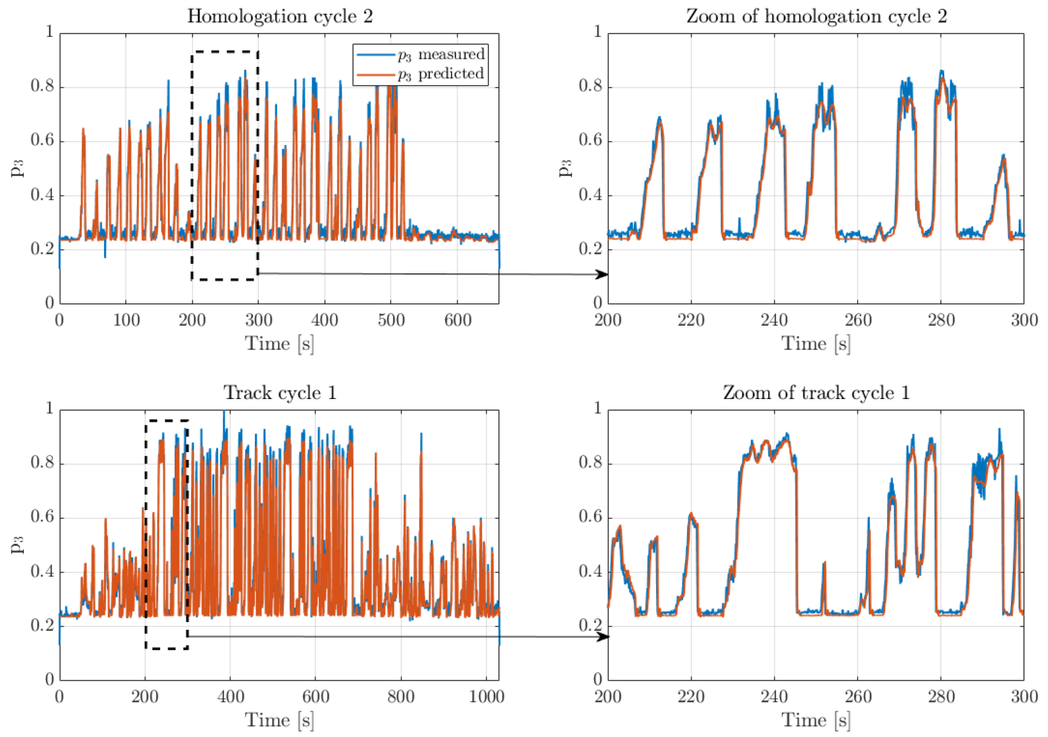
T3) and the pressure in the same position of the exhaust line (
) are the two main inputs for the calculation of the EGT at the turbine outlet (
T4). The
T3 is modelled with the hybrid approach previously described by the authors in [
32] while
is modelled with an ANN in
Section 3.1.
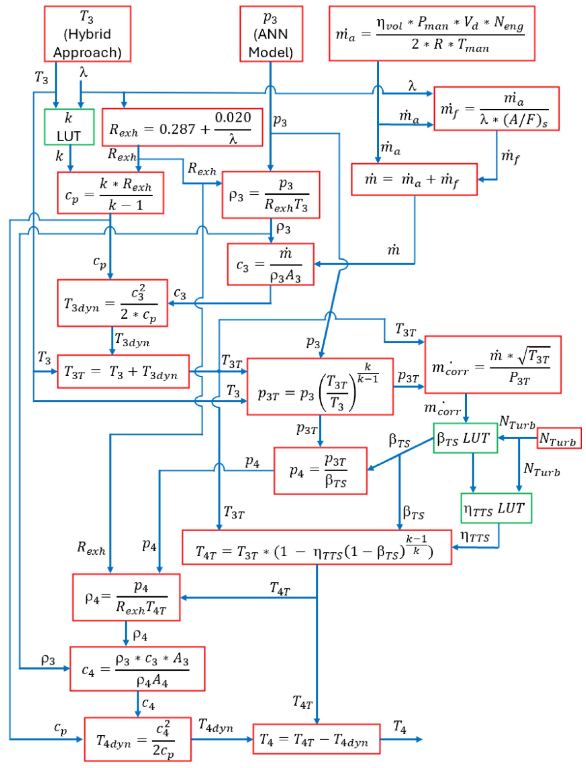
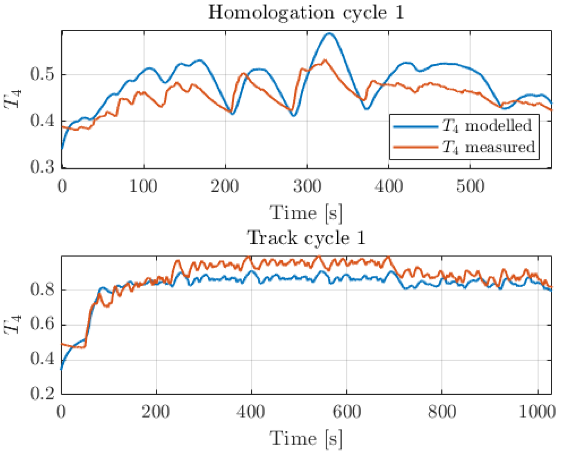
Section 3.2 deals with the description of the expansion equations used to calculate the
T4 value [
33]. The output of the
T4 model is the EGT at the turbine outlet for steady-state conditions, because all the models are calibrated with steady-state data. The
T4 value determined in this way cannot be directly compared with the
T4 measured at the bench under transient conditions, because of the TC dynamics. The TC effect is included as a first-order system, where the time constant is calibrated to minimize the error between the experimental and the calculated
T4 trace under transient conditions. The layout of the overall calculation chain is shown in
Figure 1.
In
Section 4, the validation process for both new models introduced with the present work is shown by evaluating the root mean square error (RMSE) between calculated and measured values under transient conditions for both
and
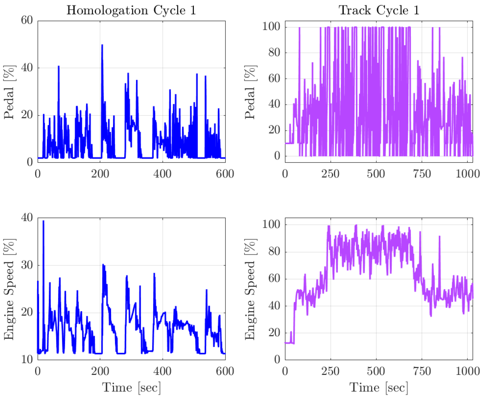
T4 estimations. Indeed, the simulation of real driving cycles represents the conditions for the final application of the
T4 model. The estimation of the complete calculation chain (composed by the
T3 model,
model, turbine model, and TC model) is directly compared with the experimental trace. The results demonstrate for six different tests that the RMSE is small and constant. This second aspect is particularly important for evaluating the extrapolation reliability of the complete simulator. Indeed, this observation suggests that similar results can be expected in further simulations.
5. Conclusions and Future Works
This study presents an innovative methodology that integrates a semi-physical turbine model for the estimation of the exhaust gas temperature at the turbine outlet using a neural network-based approach for predicting the pressure at the turbine inlet. The hybrid approach developed in this work combines the precision and robustness of physical models with the adaptability and learning capabilities of artificial neural networks. By incorporating physical models instead of relying solely on a purely data-driven, black-box approach, this methodology helps mitigate common limitations of machine learning-based models, such as poor feature extrapolation and the inability to capture physical dynamics effectively. The presented approach ensures robust and reliable model validation by testing under six different driving cycles, reproduced at the engine test cell, not used for model development or calibration. The results indicate an average root mean square error of 14%, including the initial phases of driving cycles conducted with a cold engine. Therefore, the proposed method, which integrates multiple modeling techniques, demonstrates strong predictive capability, which represents the primary objective of this research.
The results demonstrate that this methodology maintains consistency with experimental datasets and aligns with physical trends, even under operating conditions that deviate significantly from the training data. This capability is crucial for ensuring robustness and reliability of this model in real-world scenarios, including anomalous engine operations such as misfires and fuel cut-offs. These outcomes demonstrate that this new methodology can be successfully employed to estimate the exhaust gas temperature downstream the turbine, together with the implementation of a semi-physical thermocouple model.
Future developments of this work will focus on further enhancing the model’s accuracy and robustness, with a more in-depth investigation of thermal exchanges in the exhaust runner and turbine. Additionally, the exhaust gas temperature model at the turbine outlet, coupled with the previously developed engine simulator, will be extended to estimate the temperatures of various aftertreatment system components. The complete engine simulator will also be integrated with a physical catalyst model to simulate its exothermic and heat exchange reactions, enabling the prediction of exhaust gas temperatures at the catalyst inlet and outlet.


 and
and 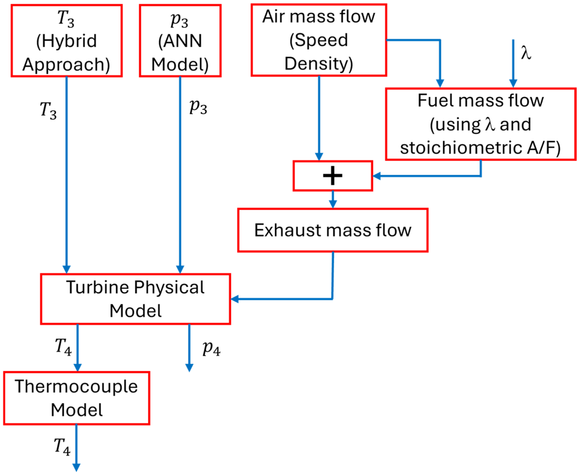
