Model Predictive Control-Based Energy Management System for Cooperative Optimization of Grid-Connected Microgrids

Abstract

This paper presents a model predictive control (MPC)-based energy management system (EMS) for optimizing cooperative operation of networked microgrids (MGs). While the isolated operation of individual MGs limits system-wide optimization, the proposed approach enhances both stability and efficiency through integrated control. The system employs mixed-integer quadratic constrained programming (MIQCP) to model complex operational characteristics of MGs, facilitating the optimization of interactions among distributed energy resources (DERs) and power exchange within the MG network. The effectiveness of the proposed method was validated through a series of case studies. First, the performance of the algorithm was evaluated under various weather conditions. Second, its robustness against prediction errors was tested by comparing scenarios with and without disturbance prediction. Finally, the cooperative operation of MGs was compared with the independent operation of a single MG to analyze the impact of the cooperative approach on performance improvement. Quantitatively, integrating predictions reduced operating costs by 19.23% compared to the case without predictions, while increasing costs by approximately 3.7% compared to perfect predictions. Additionally, cooperative MG operation resulted in an average 46.18% reduction in external resource usage compared to independent operation. These results were verified through simulations conducted on a modified version of the IEEE 33-bus test feeder.

1. Introduction

1.1. Research Background and Motivation

The increasing severity of climate change has highlighted the need for a structural transformation of global power systems to reduce greenhouse gas emissions and achieve sustainable development [1]. Consequently, the traditional fossil fuel-driven, vertically integrated energy industry is transitioning to decentralized, horizontal energy industries such as MGs, which leverage small-scale distributed resources. MGs, particularly those utilizing renewable energy resources such as photovoltaic (PV) systems and wind turbines (WT), are increasingly recognized as a solution to both promote the use of green energy and address broader environmental issues. Beyond reducing greenhouse gas emissions, these transformations can lead to a comprehensive restructuring of power systems, including the integration of energy storage systems (ESSs). A MG is defined as a smart power system that includes loads, distributed generators (DGs), and ESSs, all grouped together within a limited geographic area [2,3]. MGs have long been recognized as effective solutions for integrating these power sources into conventional power systems without causing significant disruptions [4]. In MGs, consumers can independently manage both their energy demand and surplus energy through a bidirectional communication platform and control devices [5]. MGs can either be connected to the main grid or operate autonomously. When connected to the main grid, MGs can receive additional power from the grid. However, from the perspective of sustainable development, purchasing energy from the main grid, especially when the energy is generated from non-renewable resources, should be regulated within certain limits [6]. Independent MGs must maintain sufficient levels of DGs and ESSs to enhance system reliability and ensure the quality of local loads. However, MGs based on renewable energy face operational challenges due to the intermittency and forecast uncertainty of renewable power generation [7]. To address these challenges, networking neighboring MGs has been identified as a feasible solution. According to [8,9], energy exchange and cooperation between MGs can improve the overall reliability and stability of the system.

1.2. Related Works

The study of interconnected MGs is an active and rapidly evolving research field. Recent studies have suggested that cooperative operational strategies can provide higher efficiency and economic benefits compared to the operation of a single MG. Various algorithms and optimization models have been proposed for energy management in multiple MGs (MMG). Ref. [10] introduced a centralized control model for optimal energy management in MG networks using a linear quadratic Gaussian problem formulation. The study aimed to minimize power exchanges between MGs and optimize local energy storage operations. Ref. [11] proposed a coordinated energy management strategy for networked MGs in distribution systems by formulating a stochastic bi-level optimization problem, with the distribution network operator at the upper level and MGs at the lower level. This study assumed the presence of both dispatchable and non-dispatchable DGs within the networked MGs. By transforming the nonlinear convex optimization problem into a mixed-integer linear programming formulation, the study improved computational feasibility. Ref. [12] addressed decentralized control in MG networks by enabling power exchanges between MGs to maintain local storage levels around predefined reference values. This approach employed a linear quadratic control framework, ensuring computational efficiency even in MMG systems. An integrated approach combining MG load dispatch and network reconfiguration was presented in [13], utilizing power-flow techniques to minimize the total operational cost of distribution networks incorporating MMGs. Ref. [14] proposed a decentralized optimal control algorithm for distribution management systems by modeling distribution networks as interconnected MGs. By formulating the optimal control problem as a decentralized partially observable Markov decision process, this study enabled MGs to autonomously optimize their operations while coordinating with other MGs. Ref. [15] proposed an optimal energy management strategy for cooperative MMG communities using sequentially coordinated operations. This strategy distributes computational efforts to enable optimal 24 h energy management while reducing unnecessary external trading costs. The framework integrates combined heat and power systems with ancillary internal trading mechanisms, facilitating cost-effective energy management within the MMG community. Ref. [16] proposes a hierarchical decision-making model for MMG energy management through bi-level programming. In this study, two operational models, centralized and decentralized, are presented to simulate the interaction between the MG aggregator (MA), which is the entity managing the MMGs, and the electricity market.

1.3. Research Objectives

Energy management in MGs is typically configured using offline day-ahead optimization methods, where operational plans for the following day are scheduled through a single optimization process. This method assumes perfect prediction and is modeled as an open-loop system, making it vulnerable to forecast errors. Consequently, it struggles to effectively respond to the output variability of renewable energy sources (RESs) and load demand uncertainties in real-time operating environments. Therefore, schedules generated by this static approach are likely to fail in maintaining optimal conditions in real-time scenarios where unexpected variations may occur, making them unsuitable for real-time EMSs. An alternative approach is rolling optimization, which dynamically adjusts schedules according to real-time conditions. In MG operations, MPC strategies are primarily used for rolling optimization [17,18,19]. In the MPC approach, control actions are calculated online based on system states and predictions, rather than relying on offline static control results. MPC features a closed-loop control structure, continuously adjusting control actions to compensate for forecast uncertainties. Thus, MPC is effective in formulating optimal control problems where system uncertainties exist and multi-step sequential decision-making is required.

In this paper, we propose an MPC-based cooperative EMS that extends the capabilities of conventional MPC by integrating cooperative control mechanisms. Specifically, we present a control architecture and multi-objective optimization model for a renewable energy-based MG network managed by a cooperative global central controller. The MPC approach is recognized as an optimal control method for centralized management in MG operations because it can robustly handle multi-input, multi-output functions and operational constraints [20,21]. MPC integrates predictions of future system behavior, making it particularly effective for renewable energy-based MGs and load forecasting [22]. This method utilizes forecast information on renewable generation, electrical load demand, and electricity market prices in each control step, solving the problem using a rolling horizon approach. This enables the system to manage dynamic changes and uncertainties, periodically optimizing power distribution among all controllable units to promote sustainable energy management strategies within the MG [23]. Many studies have reported that predictive model-based methods in MG operations contribute to cost minimization by reducing operational costs and enabling optimal economic scheduling [24,25,26].

This research aims to address power control issues within MG networks and maximize RES utilization to enhance the reliability of the entire network. Additionally, it explores how cooperative operational strategies between interconnected MGs can improve power system stability and economic efficiency. The focus of this paper is to achieve effective power control both locally within MGs and across the entire MG network through real-time power flow management and integrated operation of DERs, while considering uncertainties in renewable energy generation and load demand. This integrated MPC approach can effectively balance multiple objectives through appropriate parameter tuning [27]. In this paper, the multi-objective optimization problem is transformed into a single-objective optimization using a scalarization technique, specifically the cost summation method [28]. In this process, each component of the objective vector represents the cost function of an individual MG. The goal of the optimization is to minimize the total cost incurred in the MG network. This paper guarantees Pareto equilibrium by formulating a single-objective optimization that minimizes the sum of the operation costs of individual MGs, which corresponds to the sum of the components that make up the objective vector. However, this total cost minimization approach may not provide a unique solution for the optimization variables. The ratio of purchased/sold power between MGs and the main grid can be adjusted in specific solutions, which may not affect the total cost but can impact individual MG costs. To address the issue of redundancy and ensure consistent decision-making in the optimization process, a cost function related to power trading is incorporated into the formulation. This function prioritizes local optimization within each MG, thereby maintaining the integrity and efficiency of the overall optimization problem while promoting fair and equitable power distribution across the network. This paper addresses important practical considerations in MG operations. First, it provides greater operational flexibility to each MG through power exchange with neighboring MGs. Second, it ensures maximum utilization of renewable energy generated across the network. Third, it ensures that local loads can be met with minimal interaction with the main grid.

To the best of our knowledge, research considering a detailed and comprehensive MPC approach for the cooperative optimization of renewable energy-based MG networks remains a relatively new field of study. Moreover, most existing studies assume that all generators and loads within a MG are connected to a single bus, neglecting distribution network constraints such as voltage limits. As a result, the schedules obtained through these methods are unreliable and difficult to implement in real-world systems. This paper aims to bridge this important research gap in the literature. The main contributions of this thesis are summarized as follows.

• A global centralized control model has been established to efficiently manage a MG network consisting of multiple DERs and loads. Each MG is designed as a renewable energy-based MG, incorporating microturbine (MT), ESS, and local-scale power generation from RES. The complex operational characteristics and components within the MGs are mathematically formulated as constraints using MIQCP, designed to be adaptable to distribution networks of any scale.
• A synthetic forecasting technique has been proposed to generate renewable energy generation forecasting scenarios. Specifically, the probability distribution of prediction error is calculated, and added to actual generation to generate synthetic forecasting scenarios. By adjusting the added error distribution, different levels of forecast error can be simulated, allowing the robustness of the controller to be quantitatively evaluated. This method eliminates the impact of modeling errors in the forecasting module on subsequent analysis, enabling more accurate system optimization and decision-making. As a result, it distinguishes itself from conventional time series-based forecasting methods.
• MPC is employed to schedule and manage energy exchanges at the network level. All controllable devices within the MG network are optimized on a rolling basis, establishing a cooperative control framework among interconnected MGs. The proposed MPC-based cooperative EMS adopts an integrated approach that coordinates MGs within local energy systems to achieve common goals. The primary control objectives are to minimize the total operating costs, reduce energy exchanges with the main grid as much as possible, and maintain the power balance within the system.

The rest of this paper is organized as follows. Section 2 describes the proposed MMG system model and the architecture of the MPC-based EMS. Section 3 explains the method for generating synthetic forecasting scenarios of RES, incorporating realistic prediction errors. Section 4 formulates the optimization problem for power scheduling in the network of MGs. Section 5 discusses the simulation results. Finally, the conclusion is presented in Section 6.

2. System Architecture

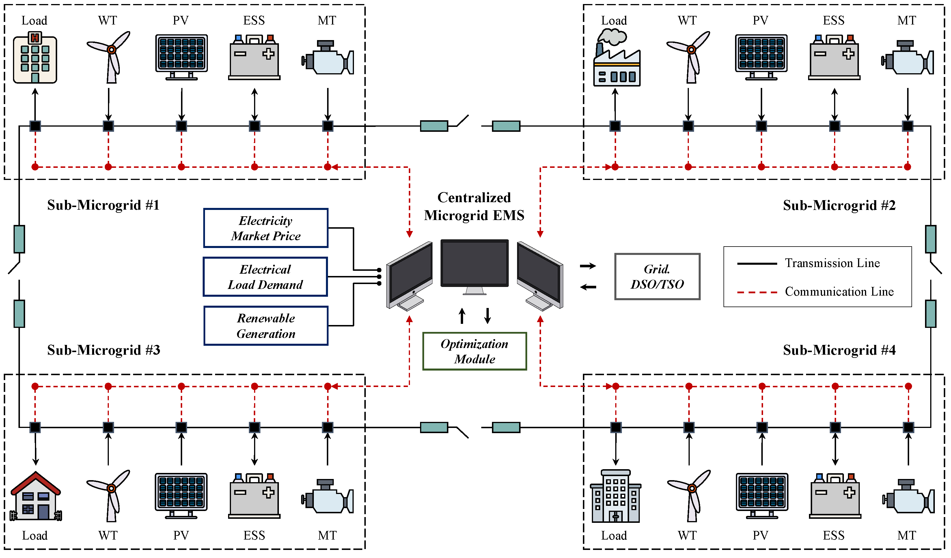
In an MMG system, each MG operates autonomously, but can perform cooperative operations with interconnected MGs when necessary. The MMG system, as illustrated in Figure 1, supports energy management under various operating conditions through this cooperative operation. Each MG is responsible for meeting its local energy demand, and when surplus energy is generated, it can either be stored in an ESS or transmitted to neighboring MGs. This flexible design allows the system to support energy production and consumption across various scenarios, dynamically adjusting according to supply and demand conditions. The energy exchange between MGs is optimized through an EMS, where each MG continuously monitors its status and maintains OPF in real time. This approach effectively manages the complex interactions that can occur within interconnected MG networks, enhancing system stability and operational efficiency.

The main objective of the EMS is to effectively maintain the power balance within the MG, which involves not only managing energy surpluses or deficits but also incorporating additional functions based on economic or operational criteria. The EMS functions as a global central control agent, enabling the optimal operation of each MG within the network while managing power coordination and exchange with regard to the relationships with the main power grid and interconnected MGs. The EMS provides high-level control by generating appropriate setpoints for all controllable devices within the system, optimizing the overall benefits of the MG network while meeting forecasted loads. Local agents within each MG include RES, MT, ESS, and load, which continuously respond to coordinated energy management commands issued by the higher-level EMS to maintain power balance. Generation of RES, electrical load demand, and electricity market price are uncertain disturbances, and their forecasts are continuously updated by the EMS based on information received from each MG.

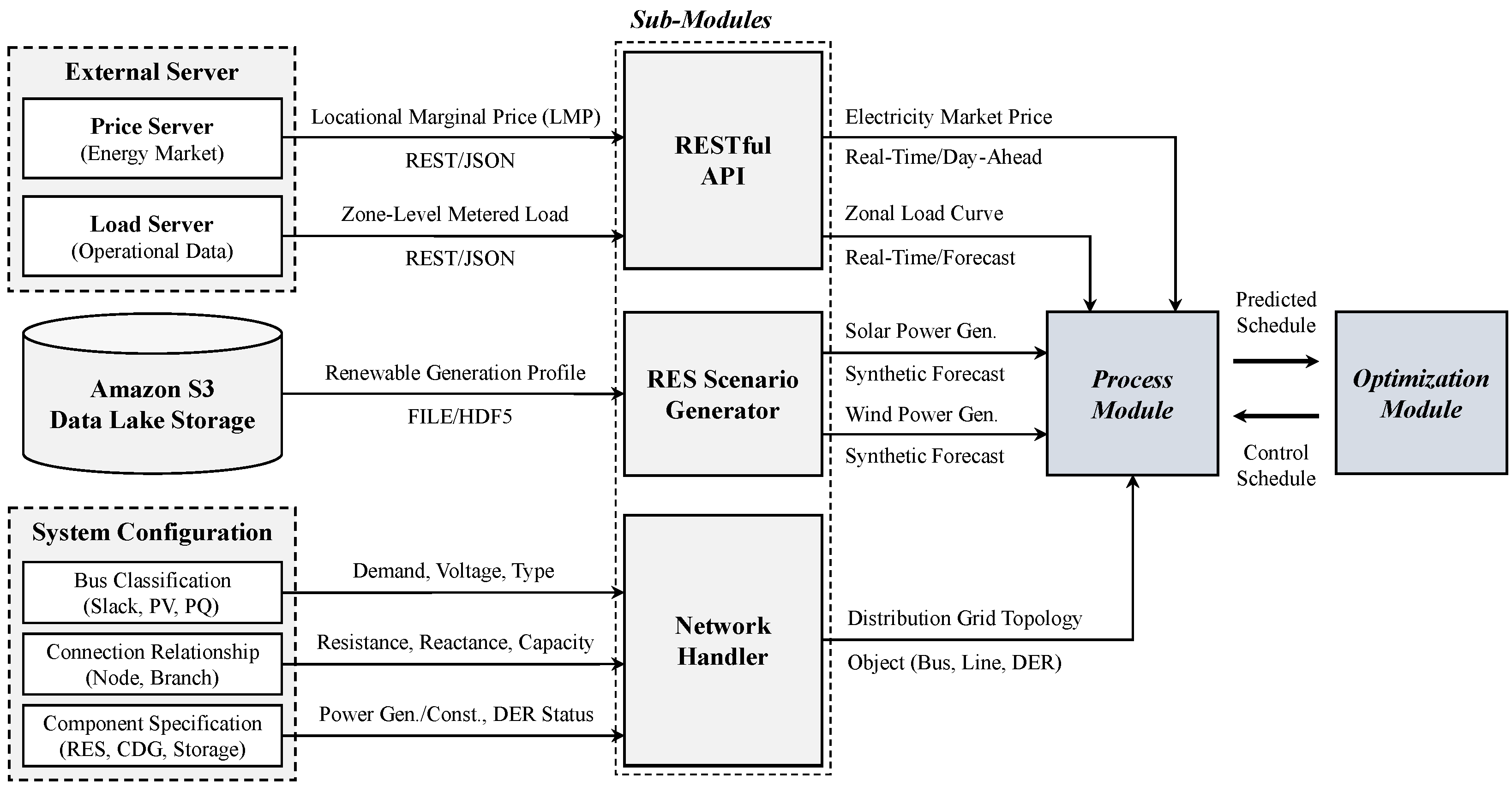
Figure 2 illustrates the communication architecture of the EMS, designed for the optimization and management of DERs within a MG. This architecture supports real-time power scheduling, DER control, and participation in the electricity market, effectively addressing the operational and economic challenges of active distribution system management. At the communication interface, the RESTful API requests structured data in JSON format from external servers. The market server provides the daily scheduled locational marginal prices (LMP) for energy trading optimization, while the load server supplies real-time measurements and the forecasted power usage data for the following day. Additionally, the renewable RES scenario generator uses historical data in HDF5 format, including time-series records of solar and wind power generation, to generate synthetic forecasts. The network handler constructs the MG network model based on system configuration. This model follows object-oriented design principles and includes individual objects representing buses, lines, and DERs to represent the physical structure of the system. These inputs are processed and integrated by the process module. The module serves as an integration interface, ensuring consistency and alignment between all forecasted and static data required for optimization tasks.

In the MPC approach, control actions are computed online based on the system state and predictions, without relying on offline static control results. The optimization model generates a sequence of control actions over a finite time horizon at each time step, but only the first step is implemented. This method operates using a rolling horizon approach, updating the available information for each MG at the next time step. The system then progresses to the next time step based on the updated state and future information, repeating the same process.

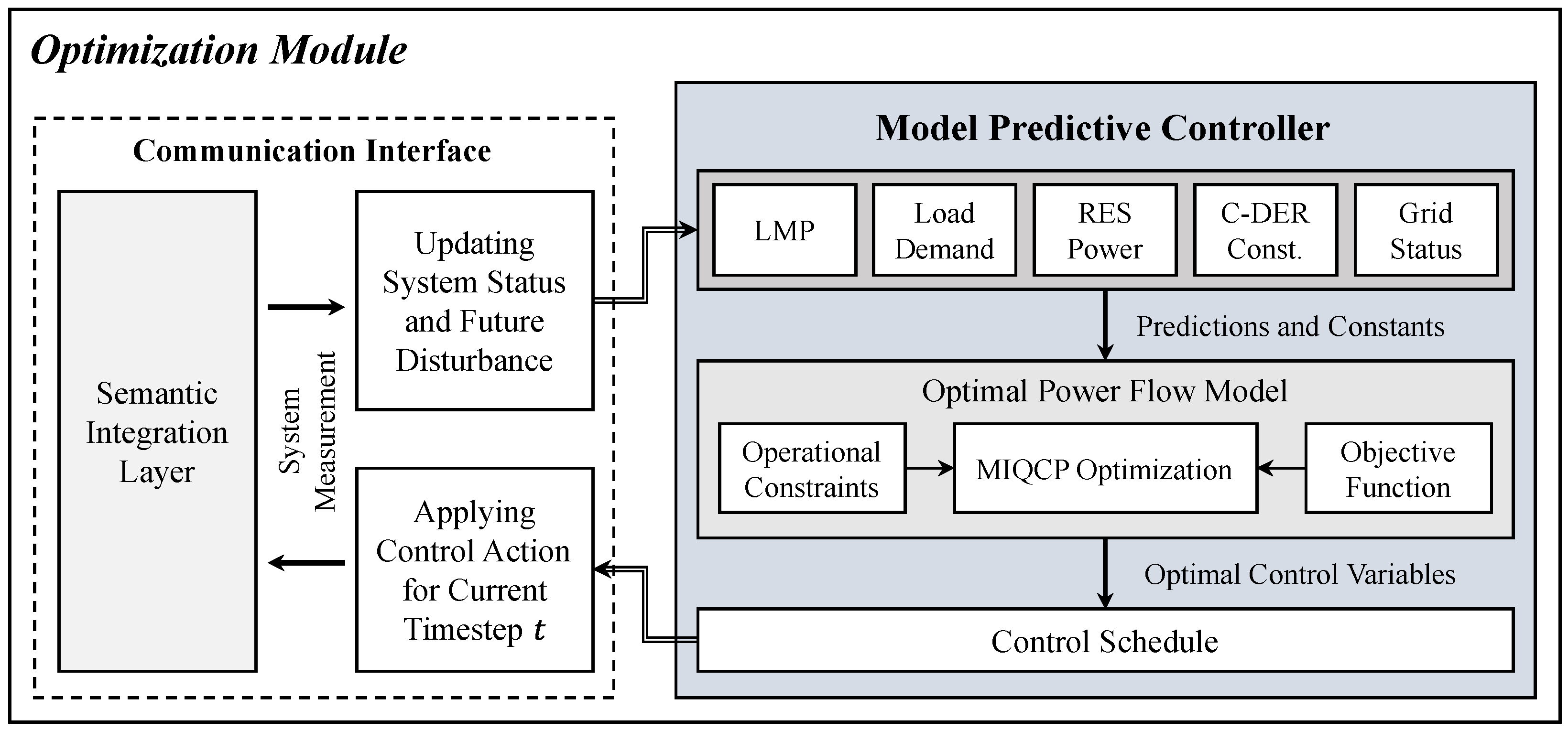
The optimization module presented in Figure 3 performs rolling horizon control, which is handled by an OPF model designed to optimize the objective function while managing operational constraints. The OPF model receives uncontrolled variables, such as renewable energy variability and load disturbances, as well as controlled variables, such as DER output and energy storage operations. The OPF model effectively manages computational complexity, and the MIQCP problem, which includes nonlinear constraints and discrete decision variables, is solved by the optimization solver Gurobi [29]. By iteratively updating its control schedule based on real-time feedback and updated forecasts, the model predictive controller ensures robust and adaptive decision-making under dynamic grid conditions. This interface facilitates seamless communication, enabling the exchange of system measurements and optimal control variables.

MPC features a closed-loop control structure, continuously adjusting control actions to compensate for forecast uncertainties. Thus, MPC is effective in formulating optimal control problems when system uncertainties exist and multi-step sequential decision-making is required. The MPC setup for optimal control problems employs a dynamic control horizon, advancing the control horizon by one step in each control iteration. The process of solving the proposed MPC-based power scheduling problem is diagrammatically represented in Figure 4. The proposed MPC schedules a 24 h period, with the prediction horizon set to 6 h and the control horizon set to 1 h.

3. Synthetic Forecasting Method

The generation of renewable energy is highly influenced by natural environmental factors, making accurate prediction a very challenging task. This uncertainty is likely to result in forecasting errors, which can significantly impact decision-making processes related to distribution system optimization. Therefore, to minimize the effect of forecasting errors on system performance, it is essential to appropriately adjust and manage the level of prediction error. In this section, we propose a method for generating synthetic forecasts that reflects various error levels based on actual renewable energy generation. The proposed method generates synthetic forecasts by adding probabilistic errors that follow predefined error distributions to the actual observations. Specifically, it is designed so that the forecasting error accumulates over time, resulting in larger errors for future time points compared to the present. The synthetic forecasts generated through this method more accurately mimic real-world conditions and minimize errors caused by the limitations of forecasting models. In this study, this method was employed to construct forecast scenarios that reflect various error levels, and the controller’s performance was quantitatively evaluated under different error conditions. The following two subsections will provide detailed explanations of the error distribution modeling method and the procedure for generating power forecast scenarios based on error levels. This method offers a tool for systematically considering forecasting uncertainty in power system operations, presenting the potential to enhance the flexibility and reliability of operational planning and control strategies.

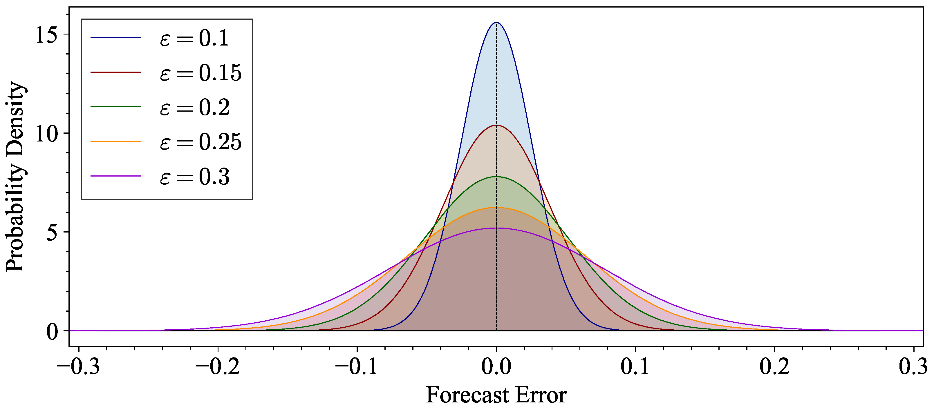
3.1. Error Distribution Model

The goal of our study is to develop a stochastic process model that can adequately represent the uncertainty of forecasts while considering non-stationarity and physical constraints. The first step in the synthetic scenario generation process is mathematically modeling the probability distribution of the forecast errors. Forecast errors tend to accumulate over time, and as errors from each time step add up, the total error in multi-step forecasts gradually increases as time progresses. In this study, to realistically reflect the uncertainty in renewable energy generation forecasts, the forecast error $e_i$ at each time step is sampled from a normal distribution $N\left(\mu ,{\sigma }^2\right)$. We assume the forecast is unbiased, meaning that there is neither overestimation nor underestimation. Thus, the mean $\mu$ of the forecast error is set to 0. The standard deviation is set to reflect the size of the error accumulated at each time step, capturing the phenomenon where forecast uncertainty increases over time. These forecast errors accumulate to form the total forecast error $S_n={\sum }_{i=1}^n{e}_i$, which follows a folded normal distribution. A folded normal distribution is expressed as the absolute value of a normally distributed variable, allowing the expected value of the accumulated error to reach a predefined error level $\epsilon$. Specifically, to ensure that the expected value of the absolute accumulated forecast error $\mathbb{E}\left[\left|S_n\right|\right]$ satisfies the target error level $\epsilon$, the following condition must be met:

$$\mathbb{E}\left[\left|S_n\right|\right]=\sigma \sqrt{{\displaystyle \frac{2n}{\pi }}}=\epsilon$$

(1)

Thus, the standard deviation $\sigma$ is determined based on the target error level $\epsilon$ as $\sigma =\epsilon \sqrt{\pi /2n}$, and the forecast error $e_i$ follows a normal distribution $N\left(0,{\left(\epsilon \sqrt{\pi /2n}\right)}^2\right)$, where, $n$ represents the number of time steps, and the standard deviation $\sigma$ decreases as the forecast period $n$ increases, ensuring that the absolute value of the accumulated error over the entire forecast period reaches the target error level $\epsilon$. The probability density functions of the proposed probabilistic error model are presented in Figure 5. This mathematical approach allows us to model how forecast errors accumulate over time and how their results reach a specific target level.

3.2. Generation of Synthetic Forecasting Scenarios

We now describe the process of generating probabilistic renewable energy generation scenarios based on the estimated forecast error distribution. To generate a synthetic forecast, it is necessary to add errors to actual generation to simulate realistic forecast scenarios. This process plays an important role in simulating various situations that may occur in actual operating environments by integrating the variability of renewable energy systems and the uncertainty of forecasts. This method allows for the emulation of forecasts with different error levels without the need for complex prediction modeling. Given the forecast horizon $t$ and the output percentage of actual generation during the forecast period $P_{1:t}=\left[p_1,p_2,p_3,\dots ,p_t\right]$, the synthetic forecast ${\widehat{P}}_{1:t}=\left[p_1,{\widehat{p}}_2,{\widehat{p}}_3,\dots ,{\widehat{p}}_t\right]$ is generated at each step by adding synthetic forecast errors as follows:

$${\widehat{p}}_j=\underset{y^{\prime }\in \left[0,b_j\right]}{argmin}\{|y^{\prime }-(p_j+\sum _{i=1}^j{e}_i)|\},j\in \left\{2,3,\dots ,t\right\}$$

(2)

The forecast error $e_i$ at each step is modeled as independent and identically distributed, following a normal distribution $N(0,{\left(\epsilon \sqrt{\pi /2t}\right)}^2)$, where $argmin$ is a function that ensures the forecast remains within feasible upper and lower bounds. In renewable energy generation, the support range of the probability distribution cannot include negative generation values or values that exceed the installed capacity, where $b_j$ is an estimated upper bound at step $j$. For WT, $b_j$ is equivalent to the installed capacity. Since the normalized output is used, this value remains constant at 1. In contrast to WT, for a PV system, $b_j$ is time-variant and is given by the power generation under clear-sky conditions at step $j$. The estimated maximum power output at each time step $j$ is calculated based on the historical observed maximum solar power for each time period.

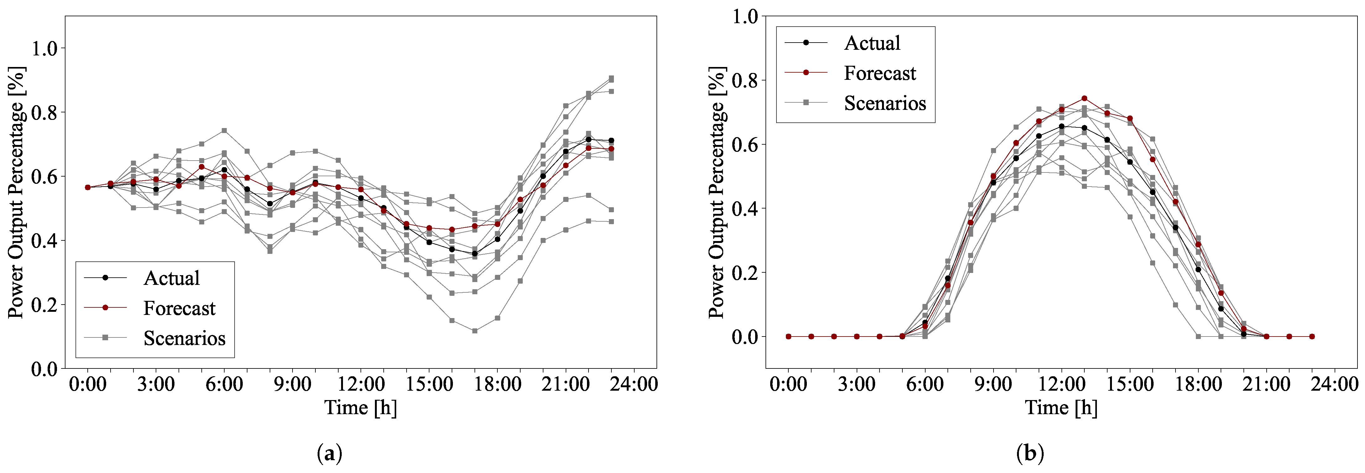
Through this process, synthetic forecasts that reflect the uncertainties that may arise in real operating environments can be generated. Figure 6 shows the daily wind and solar power scenarios generated using this method, which are compared with actual generation and forecasted generation provided by the National Renewable Energy Laboratory [30]. The error level $\epsilon$ is randomly selected between 0.1 and 0.3. This method incorporates forecast uncertainty across various scenarios, enabling system operators to develop more effective response strategies.

4. Problem Formulation

The control and management of networked MGs can be classified into two approaches: centralized and decentralized. In decentralized control, a multi-agent system is frequently utilized, where each MG interacts with autonomous agents that independently manage external power flows. However, the main challenge of decentralized control lies in efficiently achieving consensus among diverse agents. Local controllers focus on optimizing the benefits of individual MGs but may disregard the entire network behavior, leading to unpredictable outcomes. Due to the coupled nature of MGs, the local actions of one MG can influence the entire system, making it difficult to improve overall performance through collaboration among subsystems. In contrast, the centralized approach, as discussed in this study, manages and controls all MGs and the distribution system through a single control agent. Since all control actions are decided in one location, the solution is most suitable when the managing entity is a MA. This approach enables a coordinated decision-making process, where the central MG controller balances the supply and demand of all devices within the system.

4.1. System Constraints

In this section, we describe the proposed modeling configurations that ensure the optimization problem remains suitable for real-time computation. To solve the problem within the MMG system efficiently and with scalability, a robust optimization model was established using MIQCP. This approach effectively integrates complex, nonlinear constraints associated with power balance, voltage stability, and the operational limits of DERs. By formulating the OPF problem as a MIQCP, we achieved modeling of both continuous variables, such as power outputs, and discrete decisions, including the activation states of DERs and network reconfiguration options. This method enables optimal coordination among interconnected MGs, thereby enhancing system-wide efficiency and reliability. The MIQCP-based solution effectively manages dynamic interactions between generation, storage, and load demands, supporting resilient and cost-effective operations across MG networks.

4.1.1. Renewable Energy Sources

The inherently stochastic nature of RESs such as wind and solar complicates precise power output predictions. Consequently, forecasted power values, denoted as ${\widehat{P}}_{wt}\left(t\right)$ and ${\widehat{P}}_{pv}\left(t\right)$ for wind and PV systems, respectively, serve as substitutes for actual output levels. To manage variability, each RES can implement power curtailment, represented by curtailment ratios ${\kappa }_{wt}\left(t\right)$ and ${\kappa }_{pv}\left(t\right)$, which lie within the range ${\kappa }_{wt}\left(t\right),{\kappa }_{pv}\left(t\right)\in \left[0,1\right]$. These ratios specify the fraction of power curtailed relative to the forecasted values, allowing the system to dynamically adapt to fluctuations in resource availability. The curtailed power output is then expressed as:

$$P_{wt}\left(t\right)=\left(1-{\kappa }_{wt}\left(t\right)\right)\cdot {\widehat{P}}_{wt}\left(t\right)$$

(3)

$$P_{pv}\left(t\right)=\left(1-{\kappa }_{pv}\left(t\right)\right)\cdot {\widehat{P}}_{pv}\left(t\right)$$

(4)

where $P_{wt}\left(t\right)$ and $P_{pv}\left(t\right)$ denote the adjusted real power output for wind and PV generation, respectively, with curtailment ratios applied to maintain output within forecasted limits. In addition, the reactive power output of both wind and PV systems is constrained within specific bounds to ensure voltage stability and power quality. These bounds are defined as:

$$Q_{wt}^{min}\le Q_{wt}\left(t\right)\le Q_{wt}^{max}$$

(5)

$$Q_{pv}^{min}\le Q_{pv}\left(t\right)\le Q_{pv}^{max}$$

(6)

The reactive power $Q$ is further limited by the rated apparent power $S$ and the maximum active power $P^{max}$ of each resource. This constraint is represented by:

$$-\sqrt{S^2-{P^{max}}^2}\le Q\le \sqrt{S^2-{P^{max}}^2}$$

(7)

This constraint is particularly important for inverter-based RES systems, where active and reactive power capabilities are influenced by the inverter’s physical limitations and operational parameters.

4.1.2. Microturbine

MTs are integral to DG systems, offering operational flexibility to balance the intermittency of RESs and load variations. They enhance system stability and reliability by delivering both active and reactive power within defined operational constraints. At any given time $t$, the active and reactive power outputs of a MT, denoted as $P_{mt}\left(t\right)$ and $Q_{mt}\left(t\right)$, must satisfy the following bounds:

$$P_{mt}^{min}\le P_{mt}\left(t\right)\le P_{mt}^{max}$$

(8)

$$Q_{mt}^{min}\le Q_{mt}\left(t\right)\le Q_{mt}^{max}$$

(9)

where $P_{mt}^{max}$ and $Q_{mt}^{max}$ denote the maximum allowable active and reactive power capacities of the MT, respectively. To account for the characteristics of the MT, the change in power generation between two consecutive time intervals is constrained as follows:

$$\left|P_{mt}\left(t\right)-P_{mt}\left(t-1\right)\right|\le r_{mt}\cdot P_{mt}^{max}$$

(10)

where $r_{mt}$ is the ramping parameter, defined within the range $r_{mt}\in (0,1]$. Each MT is assumed to have a fixed initial fuel supply at the beginning of the time horizon $\mathcal{T}$. The total active power generated over $\mathcal{T}$ is constrained by ${\sum }_{k\in \mathcal{T}}{P}_{mt}\left(t+k|t\right)\cdot ∆t\le E_{mt}$. This constraint can be reformulated as a recursive relation by defining ${\varsigma }_{mt}\left(t\right)$ as the remaining fuel in the MT at time $t$, leading to the following energy constraint:

$${\varsigma }_{mt}\left(t\right)={\varsigma }_{mt}\left(t-1\right)-{\displaystyle \frac{P_{mt}\left(t\right)\cdot ∆t}{{\eta }_{mt}}},0\le {\varsigma }_{mt}\left(t\right)$$

(11)

4.1.3. Energy Storage System

The dynamics of the load and generators operate on significantly faster timescales and are therefore considered negligible relative to the EMS sampling interval. Consequently, the primary dynamics considered within the EMS are those of the ESS. To facilitate optimization, the ESS dynamics are modeled linearly. Since the ESS is capable of both supplying and absorbing power, discharge power injected into the grid is defined as positive, while charge power extracted from the grid is defined as negative.

The operational constraints on active and reactive power during charging and discharging of the ESS are defined as follows. The net power that the ESS exchanges with the MG, $P_{es}\left(t\right)$, is given by the difference between the discharge power $P_{es,dch}\left(t\right)$ and charge power $P_{es,ch}\left(t\right)$:

$$P_{es}\left(t\right)=P_{es,dch}\left(t\right)-P_{es,ch}\left(t\right)$$

(12)

The ESS’s active and reactive power during charging and discharging are subject to the following constraints:

$$0\le P_{es,ch}\left(t\right)\le {\delta }_{es,ch}\left(t\right)\cdot P_{es,ch}^{max}$$

(13)

$$0\le P_{es,dch}\left(t\right)\le {\delta }_{es,dch}\left(t\right)\cdot P_{es,dch}^{max}$$

(14)

$$0\le Q_{es,ch}\left(t\right)\le {\delta }_{es,ch}\left(t\right)\cdot Q_{es,ch}^{max}$$

(15)

$$0\le Q_{es,dch}\left(t\right)\le {\delta }_{es,dch}\left(t\right)\cdot Q_{es,dch}^{max}$$

(16)

where $P_{es,ch}\left(t\right)$ and $P_{es,dch}\left(t\right)$ denote the active power during charging and discharging, and $Q_{es,ch}\left(t\right)$ and $Q_{es,dch}\left(t\right)$ denote the corresponding reactive power. The binary variables ${\delta }_{es,ch}\left(t\right)$ and ${\delta }_{es,dch}\left(t\right)$, taking values in $\left\{0,1\right\}$, indicate whether the ESS is in charging or discharging mode, respectively, ensuring that power levels remain within the defined maximum capacities $P_{es,ch}^{max}$, $P_{es,dch}^{max}$, $Q_{es,ch}^{max}$, and $Q_{es,dch}^{max}$. To prevent simultaneous charging and discharging, the following mutual exclusivity constraint is applied:

$${\delta }_{es,ch}\left(t\right)+{\delta }_{es,dch}\left(t\right)\le 1$$

(17)

This ensures that only one operational mode can be active at any given time. The state of charge (SOC) of the ESS must be maintained within specific bounds to promote system stability and safety. This is enforced through the following constraint:

$${SOC}_{es}^{min}\le {SOC}_{es}\left(t\right)\le {SOC}_{es}^{max}$$

(18)

The SOC is updated at each time step based on the ESS’s current charge and discharge power, accounting for both charging and discharging efficiencies. The SOC update equation is defined as:

$${SOC}_{es}\left(t\right)={SOC}_{es}\left(t-1\right)+\left({\displaystyle \frac{{\eta }_{es,ch}\cdot P_{es,ch}\left(t\right)}{{Cap}_{es}}}-{\displaystyle \frac{P_{es,dch}\left(t\right)}{{\eta }_{es,dch}\cdot {Cap}_{es}}}\right)\cdot \Delta t$$

(19)

where ${\eta }_{es,ch}$ and ${\eta }_{es,dch}$ represent the charging and discharging efficiencies, respectively, and ${Cap}_{es}$ is the rated capacity of the ESS. The update equation reflects the net change in energy storage over each time interval $\Delta t$, ensuring that the SOC accurately reflects the ESS’s current energy state.

4.1.4. Load

To maintain the stability of the power system, the active and reactive power demands of loads must be balanced with the system’s supply capacity. In scenarios where the generation is insufficient or renewable energy output fluctuates, load reduction or adjustment through demand response (DR) programs can be implemented. This approach enables adaptive load control, which improves system reliability when demand exceeds supply capacity. In this study, the active load $P_{load}\left(t\right)$ and reactive load $Q_{load}\left(t\right)$, adjusted through DR, are defined as follows:

$$P_{load}\left(t\right)=\rho \left(t\right)\cdot P_{demand}\left(t\right)$$

(20)

$$Q_{load}\left(t\right)=\rho \left(t\right)\cdot Q_{demand}\left(t\right)$$

(21)

where $P_{demand}\left(t\right)$ and $Q_{demand}\left(t\right)$ represent the active and reactive power demands at time $t$, and $\rho \left(t\right)$ is the DR factor, indicating the proportion of the demand that is met after adjustment. The $\rho \left(t\right)$ lies within the range $\rho \left(t\right)\in \left[0,1\right]$, with values close to 1 indicating a higher proportion of demand being met and lower values indicating greater demand reduction. In instances where DR leads to reduced power delivery, the unmet power demands, representing load shedding, are given by the following expressions:

$$P_{shed}\left(t\right)=P_{demand}\left(t\right)-P_{load}\left(t\right)$$

(22)

$$Q_{shed}\left(t\right)=Q_{demand}\left(t\right)-Q_{load}\left(t\right)$$

(23)

where $P_{shed}\left(t\right)$ and $Q_{shed}\left(t\right)$ denote the active and reactive power that are not supplied to the loads due to DR adjustments. This shed power represents the quantity of load curtailed to maintain grid balance, especially under constrained generation conditions.

4.1.5. Power Grid

When a MG operates in grid-connected mode, it has the ability to conduct power transactions with the main grid, either by purchasing or selling power depending on system requirements and market conditions. These interactions are essential for optimizing the economic performance of the system. The net power transacted with the main grid is modeled as follows:

$$P_{grid}\left(t\right)=P_{pur}\left(t\right)-P_{sale}\left(t\right)$$

(24)

where $P_{pur}\left(t\right)$ represents the power purchased from the main grid at time $t$, and $P_{sale}\left(t\right)$ represents the power sold to the main grid. Both are limited by the maximum allowable transaction capacity $P_{grid}^{max}$, constrained as follows:

$$0\le P_{pur}\left(t\right)\le {\delta }_{pur}\left(t\right)\cdot P_{grid}^{max}$$

(25)

$$0\le P_{sale}\left(t\right)\le {\delta }_{sale}\left(t\right)\cdot P_{grid}^{max}$$

(26)

To ensure that the system operates exclusively in either a purchasing or selling state at any given time $t$, the binary variables ${\delta }_{pur}\left(t\right)$ and ${\delta }_{sale}\left(t\right)$, which take values in $\left\{0,1\right\}$, are employed. Specifically, ${\delta }_{pur}\left(t\right)=1$ indicates that power is being purchased from the main grid, while ${\delta }_{sale}\left(t\right)=1$ signifies that power is being sold. This setup enforces a strict operating mode, preventing simultaneous purchasing and selling actions by ensuring that only one of these variables can be active (equal to 1) at a time:

$${\delta }_{pur}\left(t\right)+{\delta }_{sale}\left(t\right)\le 1$$

(27)

For reactive power transactions, the reactive power exchanged with the main grid, $Q_{grid}\left(t\right)$, is also constrained within specified bounds:

$$Q_{grid}^{min}\le Q_{grid}\left(t\right)\le Q_{grid}^{max}$$

(28)

where $Q_{grid}^{min}$ and $Q_{grid}^{max}$ represent the minimum and maximum allowable reactive power capacities, respectively. These bounds on active and reactive power in main grid transactions ensure that the MG maintains effective power exchanges within operational limits.

4.1.6. Power Flow-Constrained Energy Balance

The power flow within the MG network is characterized by the difference between imported and exported power between nodes. The active power flow $P_{ij}\left(t\right)$ from node $i$ to node $j$ at time $t$ is defined as:

$$P_{ij}\left(t\right)=P_{import,ij}\left(t\right)-P_{export,ij}\left(t\right)$$

(29)

where $P_{import,ij}\left(t\right)$ represents the power imported to node $i$ from node $j$, and $P_{export,ij}\left(t\right)$ represents the power exported from node $i$ to node $j$. This expression models the direction and magnitude of power flow as the difference between imported and exported power. Both $P_{import,ij}\left(t\right)$ and $P_{export,ij}\left(t\right)$ are constrained by the maximum capacity of the line, $P_{ij}^{max}$, as follows:

$$0\le P_{import,ij}\left(t\right)\le {\delta }_{import,ij}\left(t\right)\cdot P_{ij}^{max}$$

(30)

$$0\le P_{export,ij}\left(t\right)\le {\delta }_{export,ij}\left(t\right)\cdot P_{ij}^{max}$$

(31)

To ensure that power is either imported or exported, but not both simultaneously at any given time $t$, the system uses binary variables ${\delta }_{import,ij}\left(t\right)$ and ${\delta }_{export,ij}\left(t\right)$, which take values in $\left\{0,1\right\}$. Specifically, ${\delta }_{import,ij}\left(t\right)=1$ allows power import, while ${\delta }_{export,ij}\left(t\right)=1$ enables power export. The following exclusivity constraint prevents simultaneous importing and exporting:

$${\delta }_{import,ij}\left(t\right)+{\delta }_{export,ij}\left(t\right)\le 1$$

(32)

The reactive power flow $Q_{ij}\left(t\right)$ is also subject to bounds that ensure it remains within the allowable limits for line $ij$:

$$Q_{i,j}^{min}\le Q_{ij}\left(t\right)\le Q_{ij}^{max}$$

(33)

where $Q_{i,j}^{min}$ and $Q_{ij}^{max}$ represent the minimum and maximum reactive power capacities of the line. Additionally, the total power transmitted along the line, represented by the sum of the squares of active and reactive power, must not exceed the line’s maximum transmission capacity $L_{cap,ij}$, governed by the binary variable ${\delta }_{ij}\left(t\right)$:

$${P_{ij}\left(t\right)}^2+{Q_{ij}\left(t\right)}^2\le {\delta }_{ij}\left(t\right)\cdot L_{cap,ij}^2$$

(34)

The binary variable ${\delta }_{ij}\left(t\right)$, which takes values in $\left\{0,1\right\}$, functions as a switching element to indicate the operational status of the line. When ${\delta }_{ij}\left(t\right)=1$, power flow is enabled between nodes $i$ and $j$; when ${\delta }_{ij}\left(t\right)=0$, no power flows along the line. This setup allows the model to reflect both physical and control-based constraints on line availability, optimizing power exchanges according to line capacity. To maintain energy balance at each node, the system must satisfy the following power flow equations, which enforce the balance of generated and consumed power by accounting for inflows, outflows, and the power flowing within the network at each node $j$. It is reasonable to assume that the line losses are negligible compared to the line power flows. Therefore, the power losses can be approximated as zero to reduce the computational complexity in power flow analysis. This approximation derives the simplified DistFlow model, specifically the linearized DistFlow model [31]:

$$\begin{array}{ll}{\displaystyle \sum _{i\in \mathcal{N}}}{A}_{ij}\cdot P_{ij}\left(t\right)+P_{wt,j}\left(t\right)+P_{pv,j}\left(t\right)+& P_{es,j}\left(t\right)+P_{mt,j}\left(t\right)+P_{grid,j}\left(t\right)\\ & ={\displaystyle \sum _{k\in \mathcal{N}}}{A}_{jk}\cdot P_{jk}\left(t\right)+P_{load,j}\left(t\right)\end{array}$$

(35)

$$\begin{array}{ll}{\displaystyle \sum _{i\in \mathcal{N}}}{A}_{ij}\cdot Q_{ij}\left(t\right)+Q_{wt,j}\left(t\right)+Q_{pv,j}\left(t\right)+& Q_{es,j}\left(t\right)+Q_{mt,j}\left(t\right)+Q_{grid,j}\left(t\right)\\ & ={\displaystyle \sum _{k\in \mathcal{N}}}{A}_{jk}\cdot Q_{jk}\left(t\right)+Q_{load,j}\left(t\right)\end{array}$$

(36)

In these equations, $A_{ij}$ and $A_{jk}$ are adjacency matrices that define node connectivity, modeling power inflows and outflows at node $j$ at time $t$. Voltage drops due to power flow in the radial network are calculated using the following voltage drop equation, which models the impact of power flow on node voltages:

$$V_j\left(t\right)={\delta }_{ij}\left(t\right)\cdot \left(V_i\left(t\right)-2\left(r_{ij}\cdot P_{ij}\left(t\right)+x_{ij}\cdot Q_{ij}\left(t\right)\right)\right)+\left(1-{\delta }_{ij}\left(t\right)\right)$$

(37)

where $V_j\left(t\right)$ is the squared voltage at node $j$ at time $t$, and $V_i\left(t\right)$ is the squared voltage of the connected parent node $i$. The parameters $r_{ij}$ and $x_{ij}$ represent the line’s resistance and reactance, respectively. The switching element ${\delta }_{ij}\left(t\right)$ accounts for connection conditions, maintaining separate voltage profiles when nodes are isolated. The voltage at each node is constrained to remain within the allowable range $v_j^{min}$ to $v_j^{max}$:

$${\left(v_j^{min}\right)}^2\le V_j\left(t\right)\le {\left(v_j^{max}\right)}^2$$

(38)

$$V_j\left(t\right)={v_j\left(t\right)}^2$$

(39)

$$v_j\left(t\right)=1,j=slack bus$$

(40)

The voltage of the slack bus is fixed at 1 p.u., serving as a reference point for the system. These voltage constraints maintain power quality and ensure reliable voltage control.

4.2. Multi-Objective Function

This section presents a centralized control problem, focusing on the economic optimization of interconnected MG networks. According to the proposed system architecture, the MA is responsible for solving the control problem using a centralized approach. In this approach, each MG must decide whether to exchange energy with other MGs. An MG only interconnects with another MG if it can achieve economic benefits equivalent to or better than operating independently.

4.2.1. Local Optimization

The objective function minimized through MPC is formulated as the aggregate of multiple cost functions representing different components of the MG. The local optimization problem for a single MG can be defined as follows:

$$J_{local}=J_{res}+J_{mt}+J_{es}+J_{load}+J_{grid}$$

(41)

The cost function $J_{res}$ for RES consists of the curtailment-adjusted generation costs for wind and PV systems. The term ${\xi }_{vwc}$ represents the curtailment cost factor for WT, while ${\kappa }_{wt}$ and ${\widehat{P}}_{wt}$ denote the curtailment ratio and forecasted power output, respectively. Similarly, for a PV system, ${\xi }_{vpc}$, ${\kappa }_{pv}$, and ${\widehat{P}}_{pv}$ are used:

$$\begin{array}{ll}{J}_{res}\left(t\right)=& {\displaystyle \sum _{k\in \mathcal{T}}}{\displaystyle \sum _{j\in {\mathcal{N}}_{wt}}}{\xi }_{vwc,j}\left(t+k|t\right)\cdot {\kappa }_{wt,j}\left(t+k|t\right)\cdot {\widehat{P}}_{wt,j}\left(t+k|t\right)\cdot \Delta t\\ & +{\displaystyle \sum _{k\in \mathcal{T}}}{\displaystyle \sum _{j\in {\mathcal{N}}_{pv}}}{{\xi }_{vpc,j}\left(t+k|t\right)\cdot \kappa }_{pv,j}\left(t+k|t\right)\cdot {\widehat{P}}_{pv,j}\left(t+k|t\right)\cdot \Delta t\end{array}$$

(42)

The cost function $J_{mt}$ represents the operational cost associated with fuel consumption. The cumulative cost is determined based on the output power $P_{mt}$ of each MT, the corresponding fuel cost $C_{fuel}$, and the efficiency ${\eta }_{mt}$.

$$J_{mt}\left(t\right)=\sum _{k\in \mathcal{T}}\sum _{j\in {\mathcal{N}}_{mt}}{C}_{fuel,j}\cdot \left({\displaystyle \frac{P_{mt,j}\left(t+k|t\right)}{{\eta }_{mt,j}}}\right)\cdot \Delta t$$

(43)

The cost function $J_{es}$ aims to minimize the economic costs associated with the use of the ESS. The lifespan of the ESS is determined by the number of charging and discharging cycles. The parameter ${CC}_{es}$ represents the capital cost of the ESS, while ${Cycles}_{es}$ denotes the number of life cycles of the battery. $C_{degr,ch}$ and $C_{degr,dch}$ are factors to penalize the degradation of the ESS in the charging and discharging process, respectively:

$$\begin{array}{ll}{J}_{es}\left(t\right)=\sum _{k\in \mathcal{T}}\sum _{j\in {\mathcal{N}}_{es}}& ({\displaystyle \frac{{CC}_{es,j}}{2\cdot {Cycles}_{es,j}}}\left(P_{es,ch,j}\left(t+k|t\right)+P_{es,dch,j}\left(t+k|t\right)\right)\cdot \Delta t\\ & +C_{degr,ch,j}\cdot {P_{es,ch,j}\left(t+k|t\right)}^2+C_{degr,dch,j}\\ & \cdot {P_{es,dch,j}\left(t+k|t\right)}^2)\end{array}$$

(44)

For load management, the cost function $J_{load}$ is formulated with a penalty related to load curtailment as follows, where the parameter $C_{voll}$ represents the value of lost load, and it is weighted by the load priority $w_{load}$:

$$J_{load}\left(t\right)=\sum _{k\in \mathcal{T}}\sum _{j\in {\mathcal{N}}_{load}}{w}_{load,j}\cdot \left(C_{voll,j}\cdot P_{shed,j}\left(t+k|t\right)\right)\cdot \Delta t$$

(45)

The cost function $J_{grid}$ represents the total cost associated with energy exchange between the local system and the main grid. The purchased power $P_{pur}$ is multiplied by the corresponding electricity purchase price ${\lambda }_{pur}$ and weighted by a temporal coefficient $\phi \left(k\right)$. This coefficient can represent priorities or preferences for energy transactions based on temporal conditions, such as peak and off-peak hours, system reliability requirements, or specific optimization goals. Similarly, the sold power $P_{sale}$ is multiplied by the sale price ${\lambda }_{sale}$ and weighted by $\psi \left(k\right)$:

$$\begin{gathered} J_{grid}\left(t\right)=\sum _{k\in \mathcal{T}}\left(\phi \left(k\right)\cdot {\lambda }_{pur}\left(t+k|t\right)\cdot P_{pur}\left(t+k|t\right) \\ +\psi \left(k\right)\cdot {\lambda }_{sale}\left(t+k|t\right)\cdot P_{sale}\left(t+k|t\right)\right)\cdot \mathsf{\Delta }\mathrm{t} \end{gathered}$$

(46)

4.2.2. Global Optimization

The global optimization of MGs is achieved through information interaction among MGs. Each subsystem needs to obtain additional information from neighboring MGs at each sampling interval. The exchanged power between MGs can be calculated as the power flow between nodes, which is located at the boundaries of the respective MGs. For each MG $i$, the cost function associated with power trading between MGs over the time horizon $\mathcal{T}$, denoted as $J_{inter}^{\left(i\right)}$, is represented by:

$$\begin{gathered} J_{inter}^{\left(i\right)}\left(t\right)=\sum _{k\in \mathcal{T}}\sum _{\begin{array}{c}j\in M\end{array}}{u}^{\left(ji\right)}\left(t+k|t\right)\cdot \left({\tilde{\phi }}^{\left(i\right)}\left(k\right)\cdot {\lambda }_{receive}^{\left(j\right)}\left(t+k|t\right)\cdot P_{receive}^{\left(ji\right)}\left(t+k|t\right) \\ +{\tilde{\psi }}^{\left(i\right)}\left(k\right)\cdot {\lambda }_{send}^{\left(i\right)}\left(t+k|t\right)\cdot P_{send}^{\left(ji\right)}\left(t+k|t\right)\right)\cdot \Delta t \end{gathered}$$

(47)

The interconnection variable $u^{\left(ji\right)}$ determines whether an active connection exists, exists between MG $i$ and its neighboring MG $j$, with $u^{\left(ji\right)}=1$ if there is a connection, and $u^{\left(ji\right)}=0$ otherwise. The cost function comprises the cost of power received by MG $i$ from MG $j$ and the cost of power sent from MG $i$ to MG $j$. The receiving cost is calculated as the product of the received power $P_{receive}^{\left(ji\right)}$, purchasing price ${\lambda }_{receive}^{\left(j\right)}$, and a time-varying weighting coefficient ${\tilde{\phi }}^{\left(i\right)}\left(k\right)$ reflecting cost preferences or priorities. Similarly, the sending cost accounts for the sent power $P_{send}^{\left(ji\right)}$, the selling price ${\lambda }_{send}^{\left(i\right)}$, and a weighting factor ${\tilde{\psi }}^{\left(i\right)}\left(k\right)$. These costs are accumulated over the entire time horizon with a temporal resolution $\Delta t$ and summed across all neighboring MGs.

The global objective function, denoted as $J_{global}$, is formulated to optimize the total energy costs across the entire MG network. The control objective within MGs involves minimizing energy costs by considering economic costs associated with DERs and the power exchanges with other MGs or the main grid. This control objective can be approached from a local MG perspective or by considering the performance of the global network. For each MG $i\in \mathcal{M}$, where $\mathcal{M}$ denotes the set of all MGs, the objective is to minimize the total of its local operational costs and power trading costs. The global objective function can be defined as follows:

$$\mathit{min}{J}_{\mathit{global}}=\sum _{i\in \mathcal{M}}\left(J_{local}^{\left(i\right)}+J_{inter}^{\left(i\right)}\right)$$

(48)

A centralized MPC calculates, at each sampling time, the sequence of inputs for all MGs to optimize the overall performance of the network. Since the decision-making process is performed globally, all MG agents collaborate to achieve the optimal solution for the entire system. This approach achieves the global optimal objective through seamless collaboration between MGs.

5. Simulation Results and Discussion

In this section, three representative case studies are presented to analyze the performance of the MMG system in terms of weather conditions, disturbance predictions, and MG operations. The analysis begins by describing the MMG system and the setup used in the simulation. Then, we present the simulation results for the three cases. Finally, the results are discussed in detail.

5.1. Simulation Setup

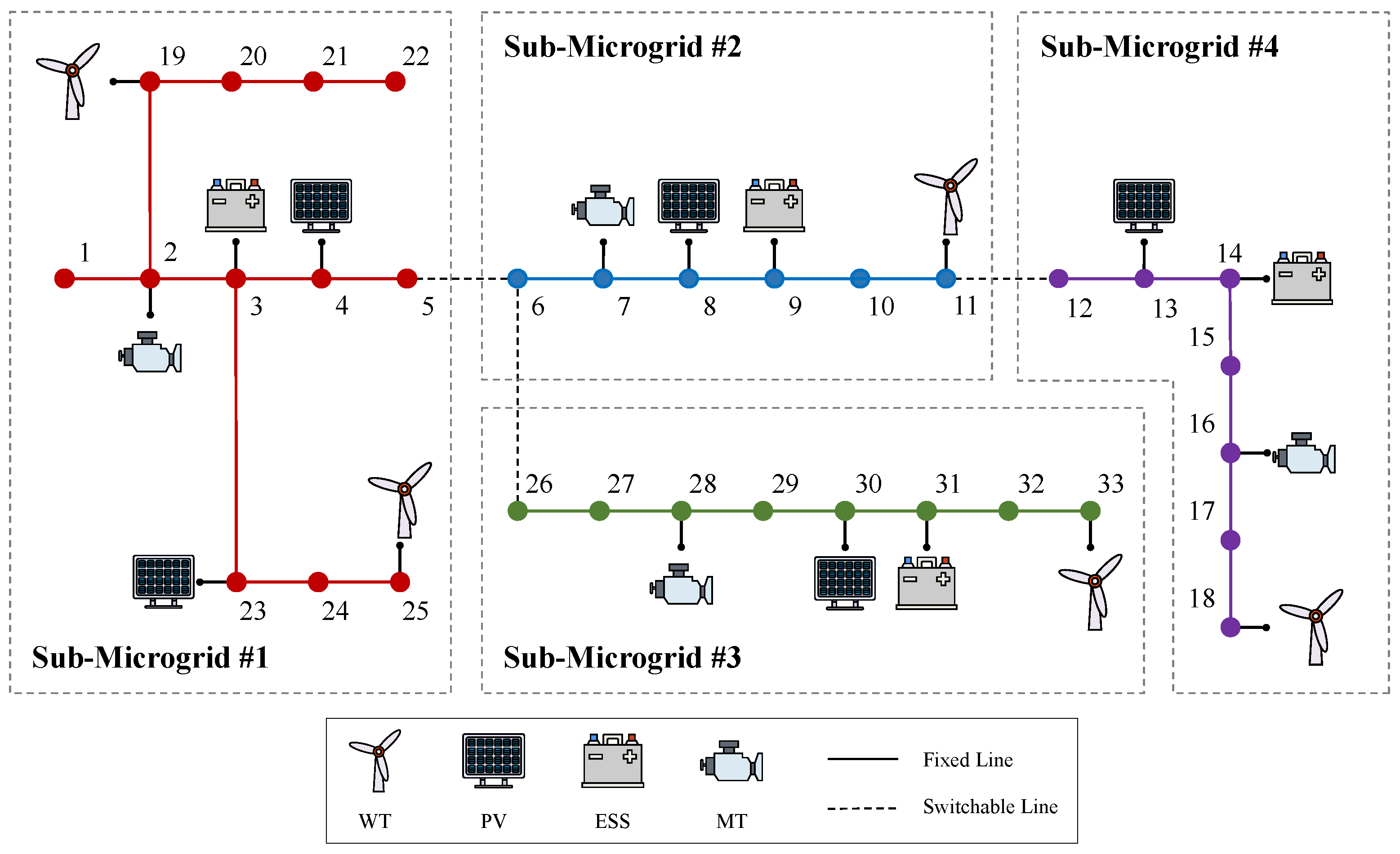
The proposed method was verified on the IEEE 33-bus system, a radial distribution network consisting of 33 buses and 32 lines. This system is a widely used standard test case in power system research, particularly suitable for evaluating the performance of distribution networks and validating algorithms. In this simulation, as shown in Figure 7, the IEEE 33-bus system was partitioned into four autonomous MGs, consistent with the approach considered in [32]. Each MG has its own PV system, WT, ESS, and MT, and is designed to receive power from external sources through its connection to the main grid when needed. The components of the MMG system and its parameters are listed in

Table 1. Components of the MMG System.

No.	Node	DER Type	Rated Capacity (kW)
MG1	19, 25	WT	600, 800
	4, 23	PV	900, 1200
	3	ESS	300
	2	MT	600
MG2	11	WT	900
	8	PV	700
	9	ESS	150
	7	MT	300
MG3	33	WT	700
	30	PV	1400
	31	ESS	200
	28	MT	400
MG4	18	WT	700
	13	PV	800
	14	ESS	100
	16	MT	200

,

Table 2. System parameters related to MT in each MG.

Parameters	MG1	MG2	MG3	MG4
${\eta }_{mt} \left(\%\right)$	34	30	32	28
$E_{mt} \left(\mathrm{k}\mathrm{W}\mathrm{h}\right)$	3600	1800	2400	1200
$r_{mt}$	0.3	0.5	0.4	0.6
$C_{gas} \left(\mathrm{U}\mathrm{S}\mathrm{D}/\mathrm{k}\mathrm{W}\mathrm{h}\right)$	0.044	0.05	0.046	0.053

and

Table 3. System parameters related to ESS in each MG.

Parameters	MG1	MG2	MG3	MG4
${\eta }_{es,ch }\left(\%\right)$	95	95	95	95
${\eta }_{es,dch }\left(\%\right)$	90	90	90	90
${SOC}_{es}^{max} \left(\%\right)$	80	80	80	80
${SOC}_{es}^{min} \left(\%\right)$	20	20	20	20
${Cap}_{es} \left(\mathrm{k}\mathrm{W}\mathrm{h}\right)$	3600	1800	2400	1200
${CC}_{es} \left(\mathrm{U}\mathrm{S}\mathrm{D}/\mathrm{k}\mathrm{W}\mathrm{h}\right)$	180	200	210	190
$C_{degr,ch} \left(\mathrm{U}\mathrm{S}\mathrm{D}/\mathrm{k}{\mathrm{W}}^2\mathrm{h}\right)$	0.00045	0.0006	0.00055	0.0007
$C_{degr,dch} \left(\mathrm{U}\mathrm{S}\mathrm{D}/\mathrm{k}{\mathrm{W}}^2\mathrm{h}\right)$	0.00035	0.0005	0.00045	0.0006
${Cycles}_{es}$	7000	6500	6750	6000

. The system operates at a nominal voltage of 12.66 kV. The total load consists of 3655 kW of active power and 2260 kVAR of reactive power. The detailed parameters of the test system are available in [33]. The system is modeled as a balanced three-phase configuration, which simplifies the analysis and ensures consistency in the simulations. This assumption excludes considerations of specific grid-forming controls among various power converters, such as the virtual synchronous generator implementations that would normally define grid-forming capabilities in converter-dominated MGs [34]. Under this assumption, detailed converter dynamics, including the formation of short-circuit currents and the operation of protection systems, are not explicitly modeled.

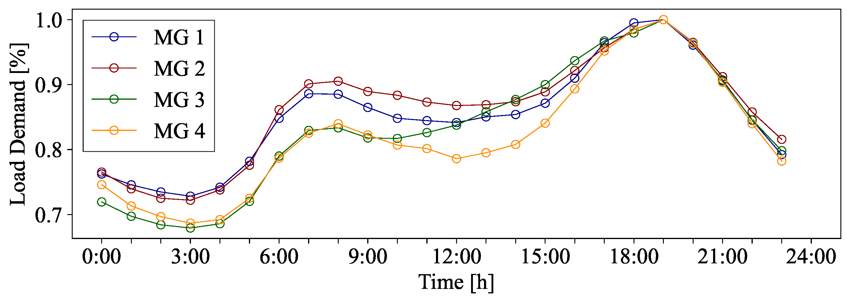
The daily load curve for each MG is modeled using four distinct load demands, as presented in Figure 8. These load demands are assigned to each MG based on the corresponding NYISO zones: CAPITAL, CENTRAL, GENESE, and HUDSON VALLEY [35]. Specifically, the actual load demands are normalized and then scaled proportionally to the rated demand of the IEEE 33-bus system. This approach replaces the previous assumption of a constant load demand, thereby incorporating realistic load variations.

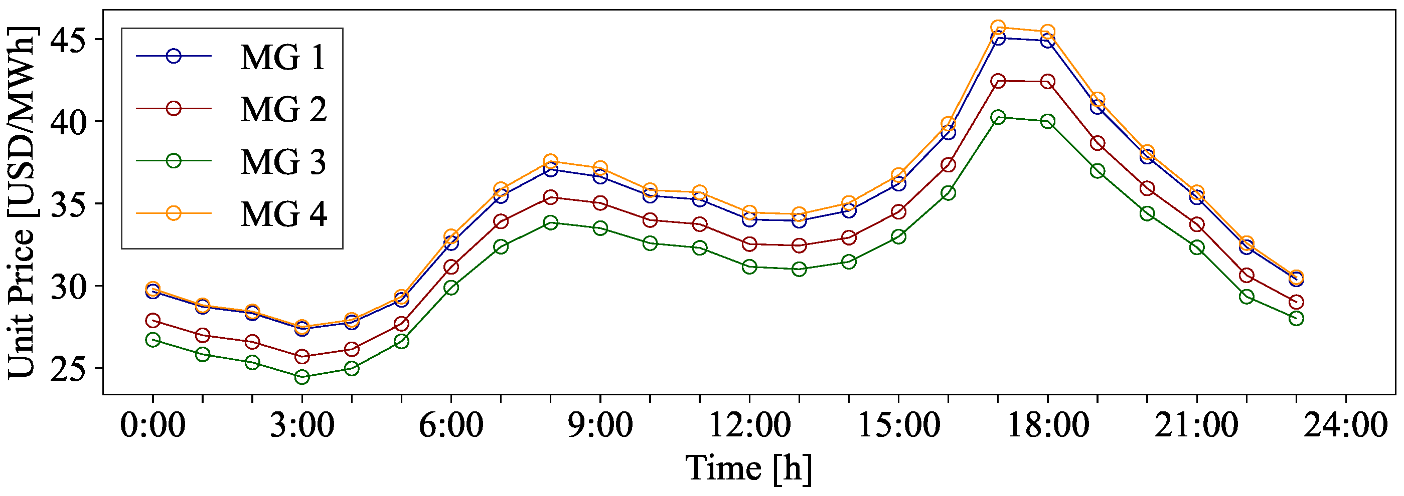
The transaction prices between the four MGs are presented in Figure 9. These prices are determined based on the day-ahead market LMP corresponding to the four NYISO regions where the load demand is established. This reflects the spatial variations in electricity market conditions and the constraints of economic dispatch models.

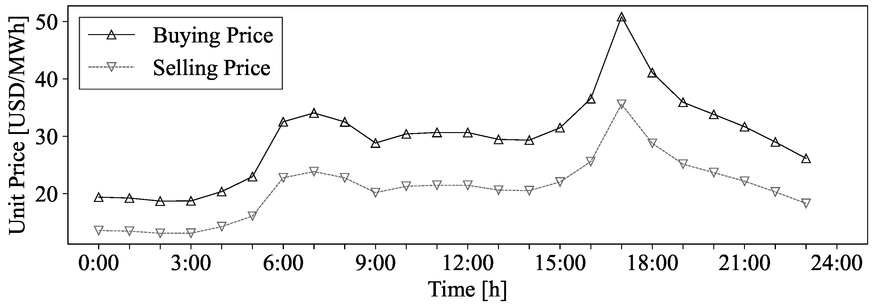
The expected costs of purchasing energy from the main grid, shown in Figure 10, are derived from the interregional energy market prices between NYISO and PJM [36]. These prices represent the cost of energy transactions with external power systems. Additionally, the price at which the MGs sell energy to the main grid is set at 70% of the buying price.

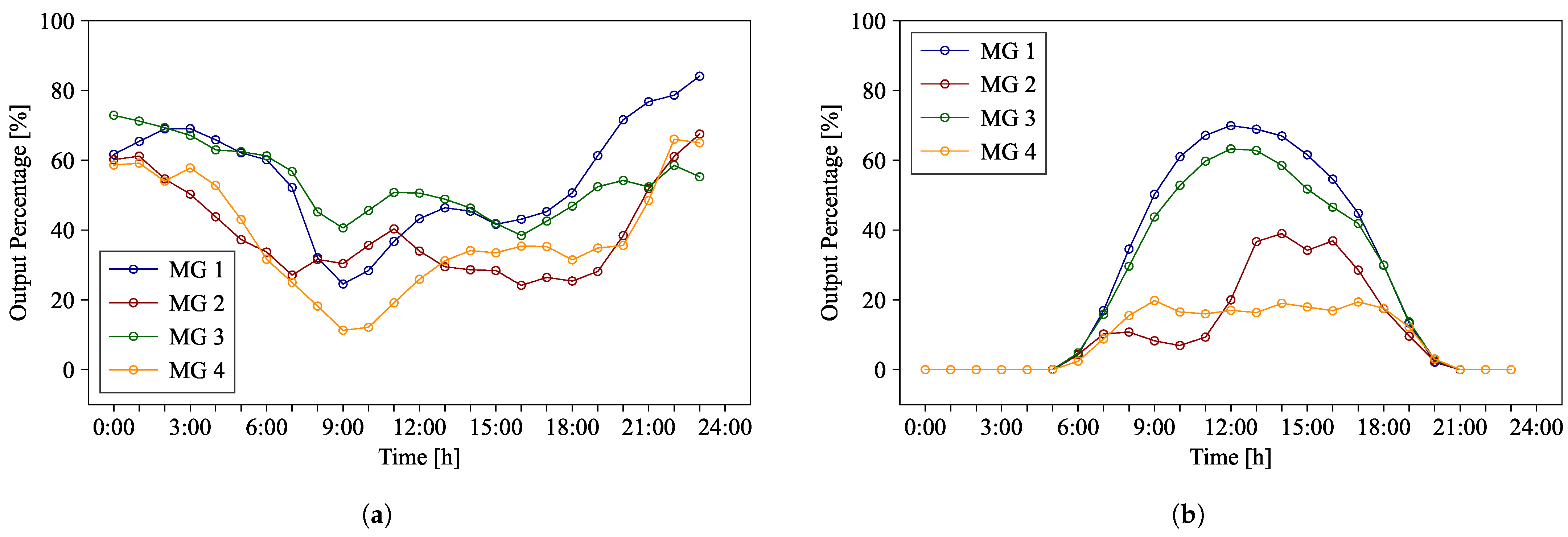
5.2. Performance Evaluation Under Different Weather Conditions

To verify the theoretical foundations, simulations were performed to evaluate the performance of the controller under different external conditions, with the same scenarios applied across all case studies. Two types of RES were considered, a PV system and a WT. MG1 and MG3 represent clear-sky conditions with stable outputs following typical solar generation patterns, whereas MG2 and MG4 simulate cloud-covered conditions with more variable outputs. Additionally, WT energy is considered under moderate wind conditions. Figure 11 shows the daily power generation of four MGs, presenting their respective output percentages.

In the simulation, four interconnected MGs are considered. The simulation results compare clear-sky and cloud-covered regions, obtaining similar results under different weather conditions. The overall conclusion confirms that the control objectives effectively minimize power exchange between the main grid and the MGs while prioritizing economic energy sources. The ESS plays a predominant role in both storing surplus energy and supplying energy deficits. The weights of the cost function can be modified to adjust these operations.

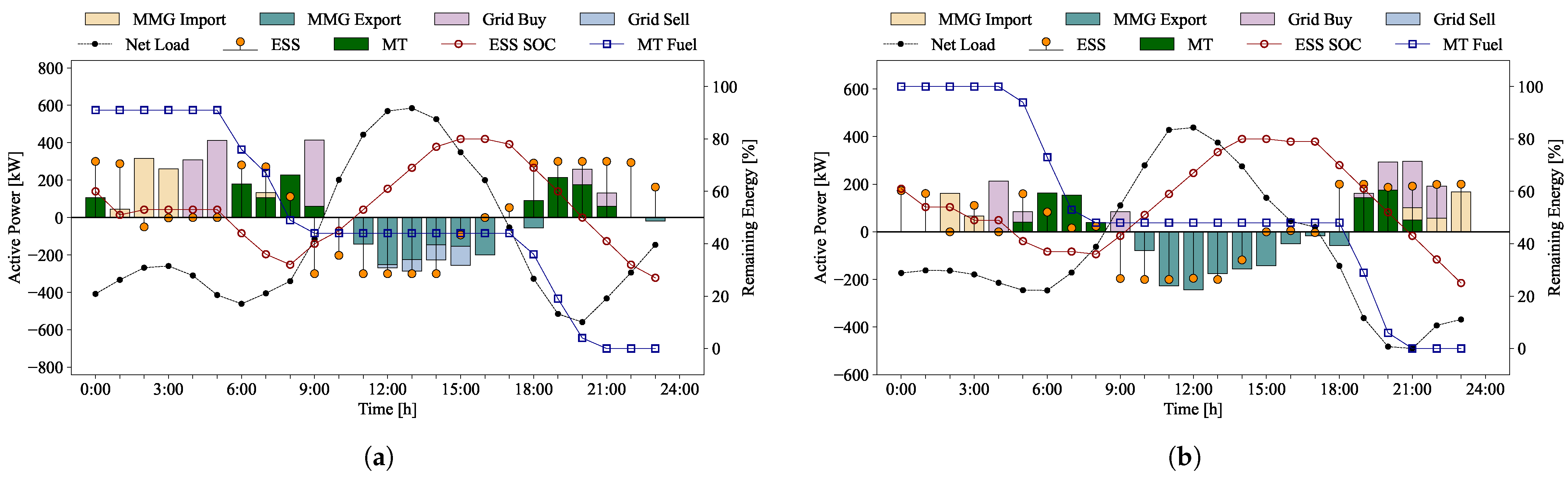
In clear-sky regions, high solar irradiation around midday results in energy surpluses, while energy deficits occur at night. The EMS manages both the ESS and MT to meet demand, as these resources are assigned low weights in the cost function and are therefore used relatively freely within operational limits. As shown in Figure 12, energy surpluses occur in MG1 and MG3 due to high solar irradiation. When the ESS in MG1 reaches its upper SOC limit of 80%, part of the surplus energy is exported to the main grid, with limited power exchange between MGs. Similarly, in MG3, when the SOC reaches its upper limit, most of the surplus energy is transferred to neighboring MGs, with negligible energy exchange with the main grid. As solar generation decreases, the ESS and MT share the load based on their respective cost function weights.

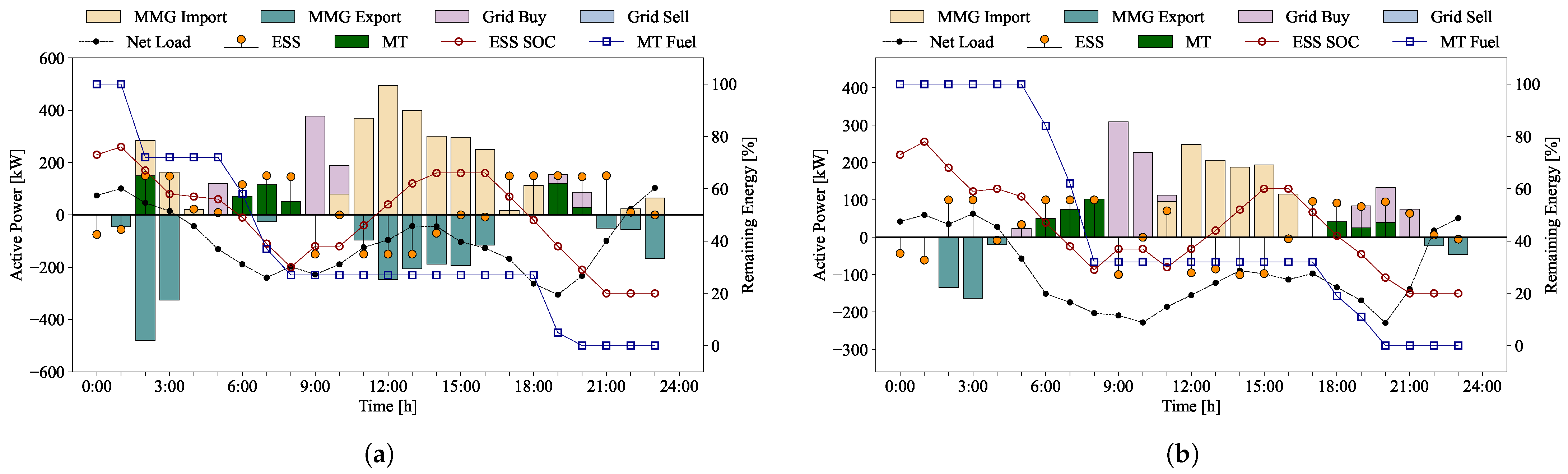
On the other hand, in cloud-covered regions, insufficient PV generation leads to unmet demand for most of the day. This energy deficit complicates MG management. As shown in Figure 13, the net load in MG2 and MG4 is predominantly negative. This deficit must be compensated through the ESS, MT, and energy exchange. In this scenario, the power exchange between MGs increases substantially. Even on cloudy days with no surplus energy, MG2 and MG4 maintain relatively high SOC levels through these energy exchanges. These results demonstrate that the MPC adapts to various scenarios, effectively managing power distribution among DERs and providing solutions that consider operational constraints and optimized operational criteria. The performance of MPC was evaluated under a wide range of operating conditions, including SOC limits of the ESS and different generation profiles, and was found to be successful. Depending on the weights assigned to each DER, the power distribution may yield different results.

5.3. Robustness Against Prediction Errors

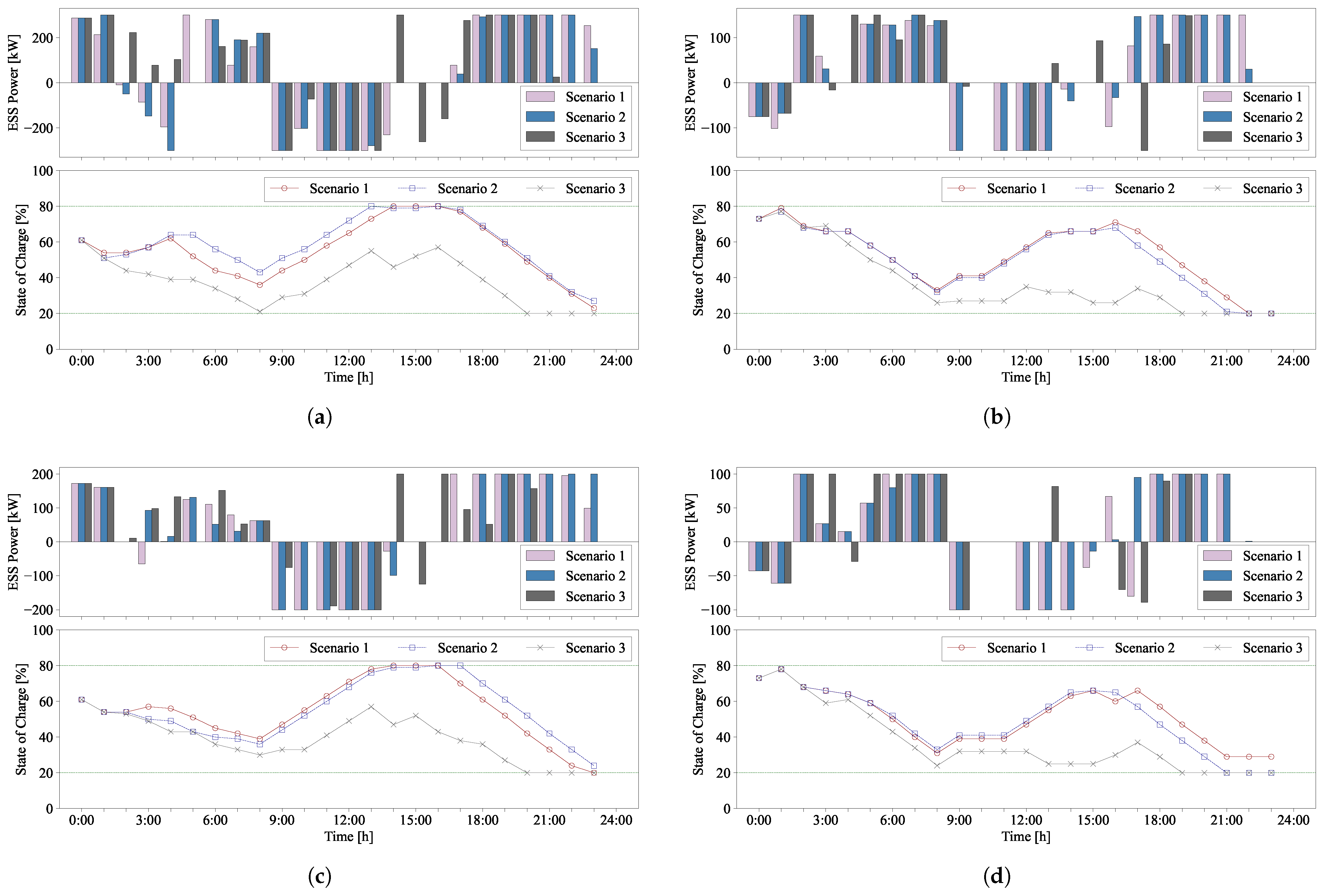
The power generated from RESs and the corresponding demand are the main disturbance factors affecting the operation of a MG. These variables cannot be directly controlled by the EMS. However, given the availability of current measurements and future predictions, MPC can anticipate system outputs within a given time horizon. This case study analyzes the impact of integrating disturbance information into MPC for MG operation. Three scenarios were considered in this study. The first scenario assumes no available future variations in disturbances. This is the most common case in MPC, where the current disturbance is assumed to remain constant over the time horizon. The second scenario represents an ideal case where perfect disturbance prediction is available, providing an upper bound on achievable optimal performance for comparison. The third scenario considers a more realistic setting where disturbance predictions are available but contain errors, reflecting the inherent uncertainty in future disturbance estimation. In this case study, disturbances are defined as the net load, calculated as the difference between generation and demand, and are measured at the current time step. The objective of this study is to evaluate the robustness of the proposed MPC approach.

Figure 14 presents the control results for ESS charging and discharging, as well as the SOC under the three scenarios. In scenarios 1 and 2, the SOC of the four MGs in the network follows a similar pattern. The prediction errors in scenario 2 cause intermittent deviations in the charging and discharging schedules; however, the trend remains comparable to that of scenario 1, which assumes perfect prediction, with an acceptable level of difference. On the other hand, in scenario 3, where future disturbances are unknown, the power system fails to proactively respond to variations, leading to ineffective ESS control. As a result, MG1 and MG3 did not charge surplus energy generated during daytime, maintaining consistently low SOC levels. Consequently, in the evening when power supply was insufficient, the ESS failed to discharge effectively, and the charging/discharging patterns exhibited abrupt changes. Such unstable operation not only degrades ESS performance but also negatively impacts its lifespan.

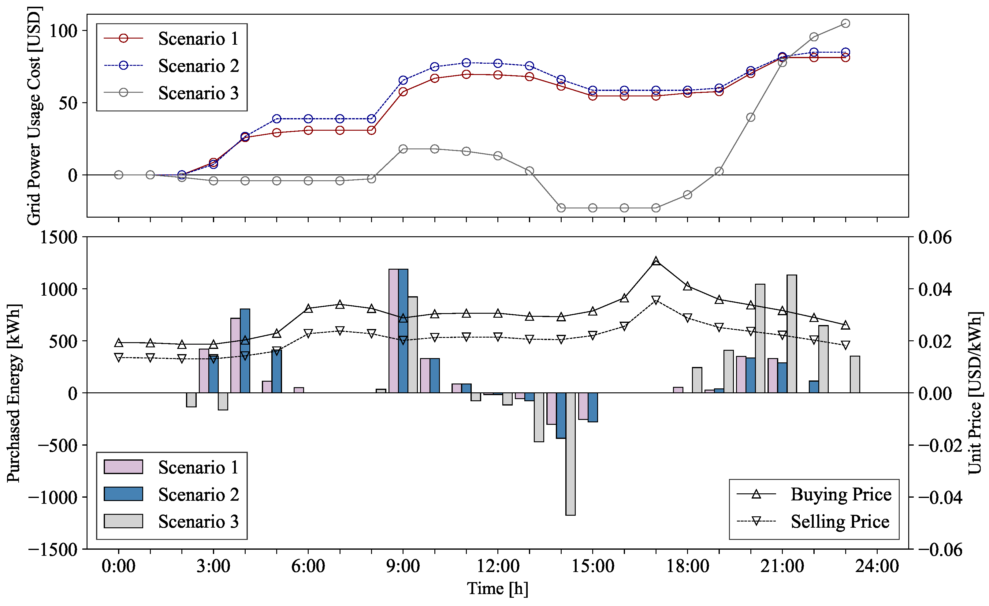
Figure 15 presents the energy exchange results with the main grid across the three scenarios. Despite the presence of prediction errors, scenario 2 operates within a similar range to scenario 1, with both cases showing a gradual increase in cumulative transaction costs. In contrast, scenario 3 experiences a sharp cost increase after 6 PM due to the lack of an optimized energy exchange strategy that accounts for electricity prices. These results reflect the limitations of static assumptions in dynamic systems. Specifically, the total costs in scenarios 1 and 2 slightly increased from USD 81 to USD 84, compared to USD 104 in scenario 3. This case study demonstrates that incorporating disturbance prediction into an MPC-based strategy can contribute to reducing operating costs by enabling proactive responses to future disturbances. Therefore, the availability of high-quality forecast information can improve the operational performance of MGs. However, even in the presence of forecast errors, the proposed MPC-based approach minimizes the impact of this uncertainty to consistently maintain near-optimal performance. This robust control strategy is particularly well-suited for real-world applications where perfect forecasting is infeasible. In conclusion, in order to effectively manage the impact of forecast errors, it should be carefully considered in MPC-based optimal control scheduling. Additionally, the selection of an appropriate prediction horizon impacts both performance and computational burden. While a longer prediction horizon typically yields better optimization results, it also increases computational complexity [37]. Therefore, the prediction horizon and time interval should be carefully determined.

5.4. Comparison of Single and Cooperative Microgrid Operation

This case study verifies the effectiveness of cooperation between MGs by comparing the performance of the proposed cooperative MG network with individually controlled MGs. It analyzes the impact of cooperative operation on each MG’s control strategy and validates the benefits of cooperative strategies for optimizing power system operation and reducing costs in the context of distributed energy management.

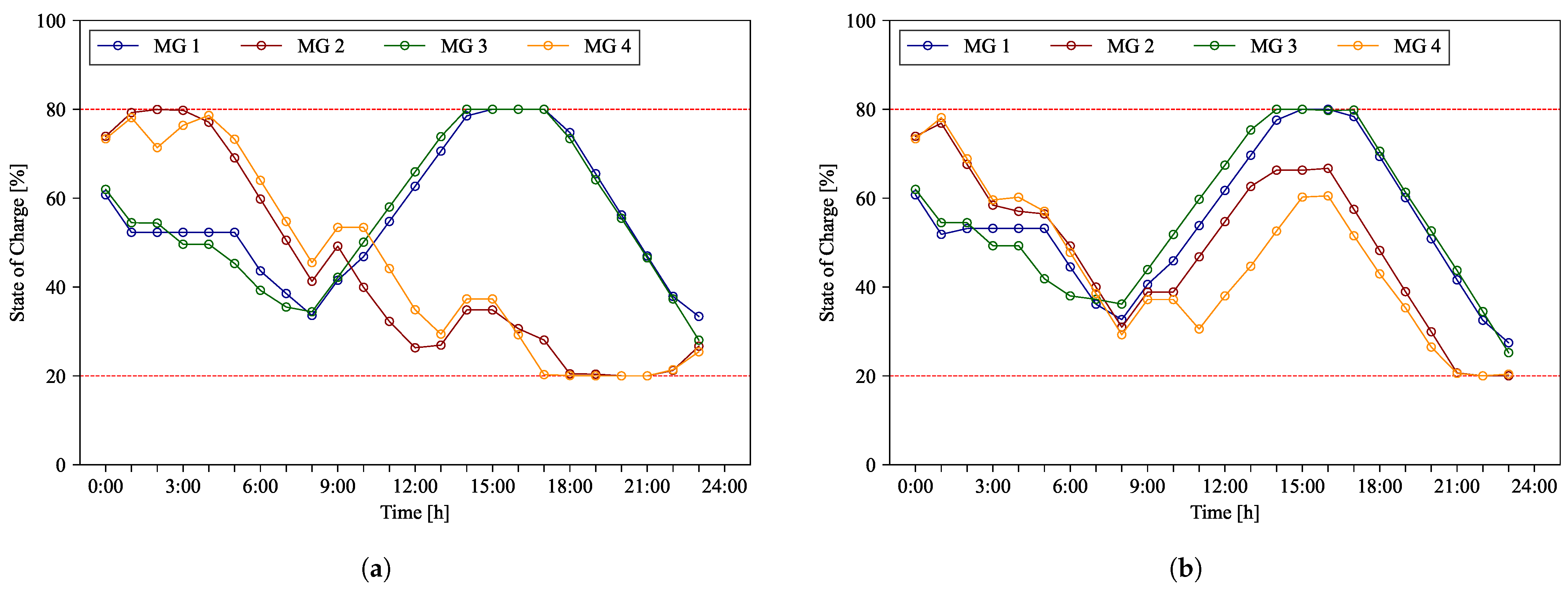
In each scenario, the SOC of the ESS is shown in Figure 16 to illustrate the differences in operational approaches. Cooperation between MGs smooths out energy usage patterns and optimizes ESS, maintaining higher SOC levels during daytime. In contrast, single MG operation shows limitations in efficiently utilizing ESS. In this scenario, each MG manages energy independently, and energy exchange is limited to interactions with the main grid. Consequently, in the single MG scenario, MG2 and MG4 experience restricted ESS charging due to insufficient PV generation, resulting in relatively lower SOC levels after 12 PM compared to the cooperative scenario. In the cooperative scenario, MG2 and MG4 could maintain higher SOC levels by receiving surplus energy from MG1 and MG3. Therefore, energy exchange between MGs can enhance the utilization of ESS.

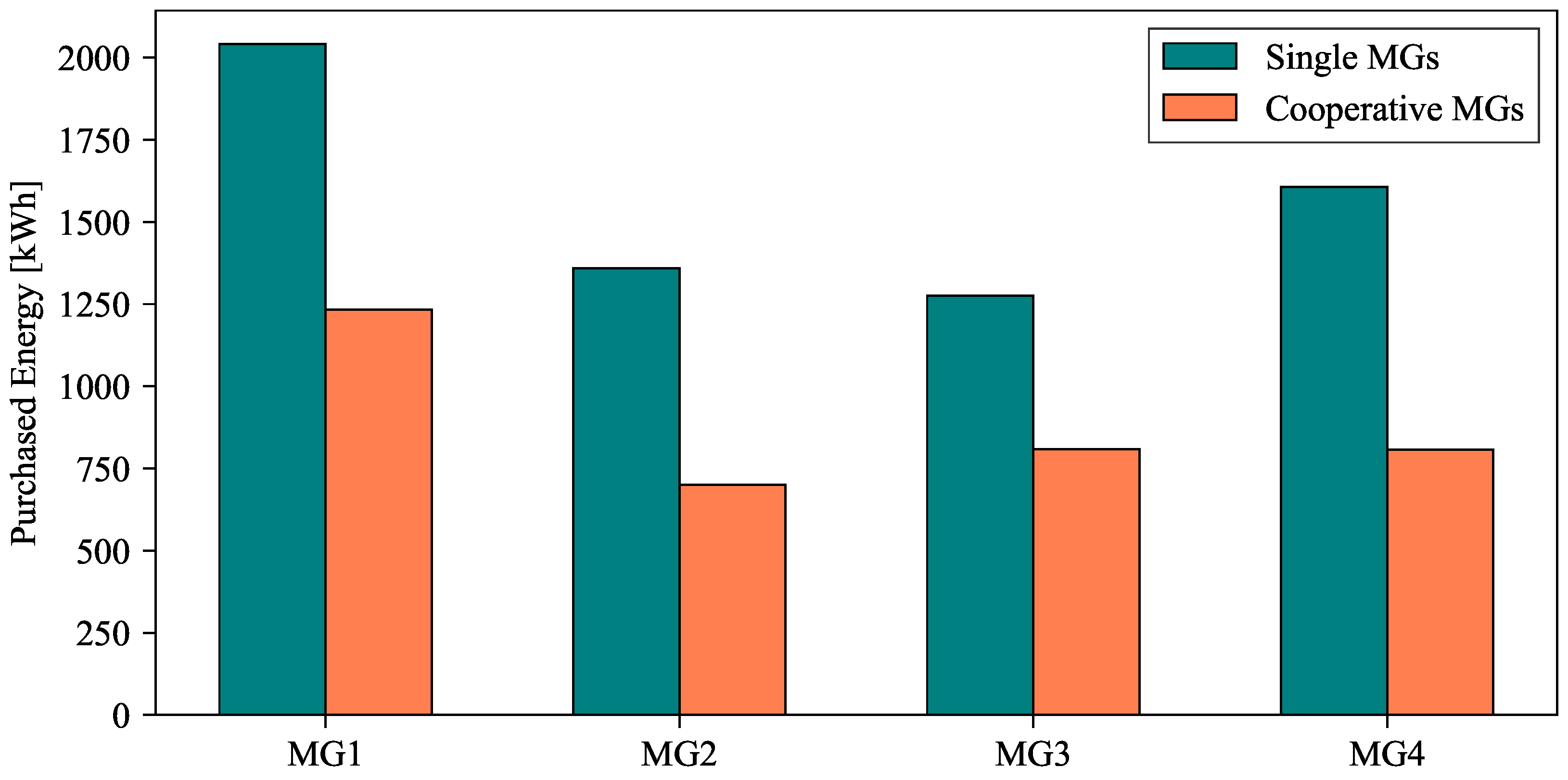
A comparison of energy purchased from the main grid in single-MG and cooperative-MG-network scenarios is shown in Figure 17. The results indicate that cooperative MGs significantly reduced energy purchases from the main grid compared to single MGs. This demonstrates that cooperation between MGs can maximize the utilization of renewable energy resources through power exchange with neighboring MGs, enhancing operational flexibility. Additionally, as shown in

Table 4. Interaction costs with the main grid in single and cooperative MGs.

	MG1	MG2	MG3	MG4
Single MGs (USD)	54.35	43.66	34.94	51.18
Cooperative MGs (USD)	33.03	18.57	23.5	22.88
Cost Saving (USD)	21.32	25.09	11.44	28.3

, it reduces dependence on expensive external energy resources, leading to substantial cost savings.

5.5. Discussion and Limitations

The simulation results lead to several important conclusions. First, it is confirmed that relying solely on RESs presents significant challenges in maintaining a stable balance between supply and demand. Both solar and wind power generation exhibit considerable temporal variability, which increases uncertainty on the supply side and can negatively impact the stable operation of power systems. Given the high dependence of renewable energy on weather conditions, there is a risk of insufficient power supply during peak demand periods. To address this issue, additional energy resources are necessary to compensate for the intermittency of renewable energy, alongside strategies for their efficient management. In this study, ESS and MT effectively fulfill this role, helping to mitigate supply–demand imbalances, a pattern consistently observed across all MGs. Second, the MPC approach demonstrates robustness against forecasting errors and provides cost-saving benefits, even in scenarios characterized by high forecasting uncertainty. Therefore, this study concludes that real-time dynamic scheduling is highly effective in improving economic efficiency and addressing forecasting uncertainty in power system operations. The MPC approach has proven to be a reliable solution for ensuring the economic efficiency of power systems, even under conditions with significant forecasting errors. Finally, the results highlight that power trading among interconnected MGs enhances operational flexibility and plays a critical role in cost optimization. These power transactions maximize the utilization of renewable energy resources and contribute to improving economic efficiency. Furthermore, the importance of dynamic interactions and power trading with the main grid was identified as a key factor in ensuring both stability and economic efficiency in grid operations. These interactions help resolve supply–demand imbalances and emphasize the need for rolling optimization techniques to minimize operational costs. Collectively, these findings suggest that managing the variability of renewable energy and enabling flexible grid operations through power trading are essential components of future energy management strategies.

However, the centralized control approach in the proposed MG cooperation model presents several limitations. First, a failure in real-time communication could have a catastrophic impact on the overall system operation. Second, as the system scales, the computational burden on the central controller increases sharply, reducing the efficiency of real-time control. Third, there is a complexity issue wherein the central controller must collect and process information from all DERs and the distribution network in real time. Additionally, a centralized system is vulnerable to operational disruptions caused by a single point of failure, which could negatively affect the reliability of the entire MG network. The current power industry faces challenges in expanding large-scale power plants due to greenhouse gas reduction goals, depletion of fossil fuels, and stricter nuclear regulations, further highlighting the limitations of centralized power systems. To overcome these drawbacks of the centralized approach, the implementation of a distributed MPC control strategy is considered a promising alternative. The distributed control approach provides a framework in which each MG maintains a degree of autonomy while coordinating with neighboring MGs to achieve global objectives. This method reduces communication burdens, minimizes the risk of single-point failures, and enhances system scalability. However, it should be noted that the distributed approach may achieve a lower level of optimality compared to the centralized approach.

6. Conclusions

This paper proposes an MPC-based EMS for optimally coordinating power exchange within a MG network sharing DERs. The study focuses on global control to maximize benefits at the network level. The proposed method integrates future information on MG states, renewable resource production, load demand, and electricity market prices into the MPC to address the optimization problem, effectively handling inevitable disturbances and prediction errors. The optimization model satisfies power flow constraints in the distribution system while integrally managing the operation of DG, ESS, and loads. To this end, the problem is formulated as a MIQCP to efficiently address complex constraints. A stochastic approach introduced to model the uncertainty of renewable energy generation provides realistic prediction scenarios, enabling analysis of the impact of forecast errors on controller performance. Simulation results demonstrate that the proposed network-based MG operation offers economic advantages over independent operation. Specifically, cooperative operation among MGs effectively addresses energy surplus or deficit issues caused by the unpredictable behavior of RESs, providing significant benefits compared to individual MG operations. An analysis of the impact of prediction uncertainty on the optimal control schedule further validates the robustness of the proposed approach. Although the proposed model relies on approximations due to certain simplified assumptions, it is highly likely to remain within specified limits when applying setpoints to real physical systems.

Future research will consider several key directions to enable practical system implementation. First, we plan to enhance the grid-forming capabilities of RESs to improve the integration and control of DERs. This will contribute to effectively managing the high uncertainty and intermittency of volatile renewable energy. Second, more sophisticated modeling will be pursued to more accurately reflect the physical characteristics and constraints of the system. In particular, we aim to explore the application of efficient optimization algorithms, such as the alternating direction method of multipliers, for large-scale distributed MPC implementation. Third, we intend to validate the proposed control strategy and evaluate its performance in real-world environments through hardware-in-the-loop simulations. This will be a critical step in confirming the effectiveness of the proposed approach in actual MG settings. Finally, developing MG operation strategies that account for policy support, such as the “Special Act on the Promotion of Distributed Energy” in Korea, represents an important future research direction. This will enhance the feasibility of MG networks not only from a technical perspective but also from the policy and economic standpoints. This study potentially suggests that the use of renewable energy can reduce dependence on fossil fuels and decrease CO₂ emissions, but it does not provide specific quantitative analysis. However, quantitatively assessing environmental impacts is essential for understanding the overall performance of MG systems. Therefore, future research should include comprehensive evaluations that incorporate these environmental impacts, which will contribute to the transition to sustainable energy systems.