Quantitative Difference Between the Effective Inertia and Set Inertia Parameter of Virtual Synchronous Generators

Abstract

Virtual synchronous generators (VSGs) have been developed to mitigate the increase in the rate of change of frequency (ROCOF) in power systems by replacing synchronous generators (SGs) with inverter-based resources. VSGs mimic the dynamics and control of SGs; however, the mechanical delay typical of an SG’s turbine is often excluded, limiting improvements to the VSG’s response. The fast frequency response (FFR) of VSGs can help reduce ROCOF and enhance emulated inertia. This implies that the effective inertia (EI) of VSGs can exceed the set inertia parameter, posing challenges for operators in allocating sufficient VSG capacity considering the inertia required for stable operation. In this study, we quantitatively analyzed the difference between the EI of a VSG and the set inertia parameter by separating the active power output into inertia and governor responses. The quantitative analysis revealed that when the VSG provides FFR within the inertia-time domain, the EI exceeds the set inertia parameter. Furthermore, the sensitivities of the VSG set parameters and VSG capacity ratio, which is related to synchronizing power coefficients and the initial sharing ratio, for the EI were analyzed. These factors were theoretically considered, and the simulations validated their characteristics.

1. Introduction

The high penetration of inverter-based resources (IBRs) in electric power systems has reduced the total physical inertia in these systems due to the disconnection of many synchronous generators (SGs) [1]. This reduction in physical inertia weakens frequency stability. In low-physical-inertia power systems, disturbances (e.g., a generator trip) degrade frequency metrics such as the rate of change of frequency (ROCOF) and maximum deviation [2]. These metrics are widely used as thresholds for protection functions of power system devices [3]. Virtual synchronous generators (VSGs) have been developed to address the decline in physical inertia. VSGs emulate SG characteristics in IBRs and can enhance power system stability as a voltage source in a mechanism similar to SGs [4,5,6,7,8,9,10,11,12,13]. These developments and evaluations have often been conducted in simple-modeled power systems with one generator, one VSG, and one load [14,15]. When introducing novel technologies like VSG, basic studies in simplified systems serve as a foundation for later, more complex real-world applications.

From an operation and planning viewpoint, operators must determine appropriate generator parameters for startup, shutdown, and control to ensure frequency stability. For ROCOF, they have traditionally used the summation of the physical inertia of SGs connected to the grid because the ROCOF is assumed to depend on total SG physical inertia. For instance, in the recently proposed frequency-constrained unit commitment, the total physical inertia is utilized as a frequency stability constraint for ROCOF [16].

In contrast to SGs, VSGs can respond to frequency variations and change their output within the “inertia-time domain”, which is the time window immediately after a disturbance, approximately 100–500 ms. This is achieved by fast frequency response (FFR), which is a no-delay governor response of the VSG [17,18]. Relying solely on the conventional concept of inertia, which references only the VSG’s set inertia parameter and the SG’s physical inertia, may underestimate the additional FFR contribution from VSGs. This underestimation can lead to an overestimation of the required generator capacity and, consequently, result in less economic operations.

Accordingly, accurately evaluating the contribution of VSGs to ROCOF, including FFR, is essential. In real-time, measurement-based stability assessments, the EI of a power system is often derived from measured ROCOF and has been widely investigated [19]. Moreover, recent studies have introduced various methods to calculate system EI and frequency support capability [20,21]. For instance, ref. [22] applied the SG swing equation to measured frequency data to determine total system EI, whereas [23] used actual energy outputs and demonstrated how they align with system inertia requirements.

Although existing methods capture both inertia parameters and the FFR effect in total system EI, accurate estimation of each generator’s effective inertia remains crucial for operational planning [24,25]. This requires a theoretical causal analysis and a quantitative assessment of EI that incorporates FFR. From the perspective of FFR’s contribution to EI, ref. [26] demonstrates that even an FFR-only device has effective inertia, derivable from an energy perspective at the frequency nadir. Furthermore, ref. [27] noted that a droop-controlled inverter (i.e., a grid-forming inverter including only FFR control) also exhibits EI and thus affects ROCOF. In VSG operational planning, it is essential to evaluate the EI of a generic VSG control scheme—including both inertia response and FFR—to clarify how EI may differ from the set inertia parameter. While prior studies note that FFR can cause the EI to exceed the set inertia parameter, few provide a theoretical explanation of why or how different factors influence FFR’s contribution. Thus, we aim to fill this gap by providing both a theoretical framework and a sensitivity analysis that reveals the primary factors influencing EI. As many state-of-the-art VSG control methods build upon the generic VSG control [28,29,30,31], developing an analytical approach for generic VSG’s EI is fundamental for assessing and refining a broad range of VSG control strategies and parameter designs.

Therefore, the goal of this paper is to quantitatively analyze the EI of a VSG by focusing on its difference from the set inertia parameter and the physical inertia of an SG using a generic VSG model. To achieve this goal, the EI of the VSG was calculated based on the SG swing equation, and the ROCOF was obtained from time-domain simulations in which the VSG was connected to a system comprising SGs. To investigate the contribution of FFR to the VSG’s EI, we examined each generator’s active power output from the inertia response, governor response, and FFR. We also considered the VSG’s set parameters and its capacity ratio in the power system, as these factors may vary in operation and planning. The novelty and contribution of this study is the examination of the difference between the EI and set inertia parameter by analyzing FFR characteristics through sensitivity analyses, demonstrating how FFR depends on parameter settings and synchronizing power coefficients. Note that while various VSG control schemes exist, we employed this generic model to clarify the underlying mechanisms of inertia emulation and FFR.

The main contributions of this study are as follows:

• We theoretically and quantitatively demonstrated that the EI of a VSG with an FFR can exceed the set inertia parameter because the FFR provides additional output in the inertia-time domain in an SG-VSG hybrid system.
• We conducted a sensitivity analysis of the effects of the set parameters in the VSG active power control on the EI value obtained from the developed EI equation.
• We conducted a sensitivity analysis of the effect of the VSG capacity ratio in the power system on the EI value in terms of the initial load share between the generators owing to the synchronizing power coefficient.

Note that the following key terms in this paper are defined as follows:

• – Effective inertia (EI): The inertia value per unit capacity of generators, back-calculated from the rate of change of frequency (ROCOF).
• – Set inertia parameter: The inertia value specified in the VSG’s inertia emulation block.
• – Fast frequency response (FFR): The VSG’s governor controls without delay (proportional control), acting more rapidly than the conventional SG governor.

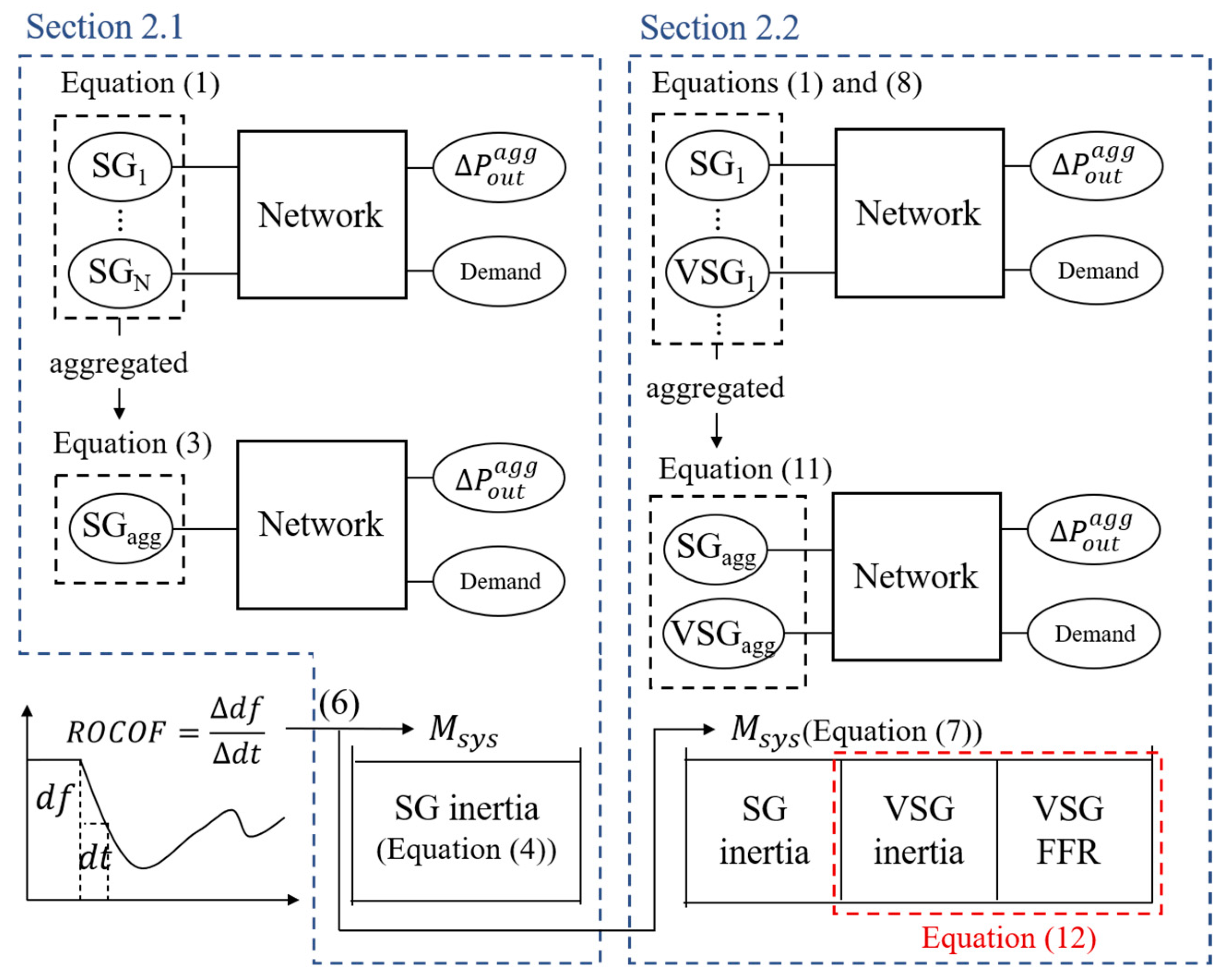
The remainder of this paper is organized as follows: Section 2 defines the EI based on the relationship between the inertia constants of SGs and the ROCOF. Section 3 explains the factors that can affect the EI values of VSGs. Section 4 presents the case study settings, including both the modeling details and the calculation process used for validation of the results. Section 5 presents the results and analysis of the case study obtained through Section 4. Finally, Section 6 concludes this study.

2. Definition of Practical Inertia on the ROCOF

In this section, we theoretically define the EI of VSGs using the conventional theory of the relationship between the ROCOF and physical inertia of SGs. This approach clarifies the EI definition in our study and highlights the factors considered in the subsequent sensitivity analysis. The key concept is that VSGs can provide not only an inertia response but also an FFR that effectively alters the ROCOF during the inertia-time domain. This results in an EI that can be higher than the set inertia parameter. Figure 1 illustrates the overall process for deriving the EI from the ROCOF for both conventional SGs and SG–VSG systems, highlighting that the SG’s physical inertia enters directly into the ROCOF equation, whereas the VSG’s inertia is modified by the FFR term. Figure 2 conceptually shows how active power dynamics can be changed by the VSG’s FFR, thereby influencing their EI.

2.1. Physical Inertia and ROCOF of SGs

This section describes the frequency variation in power systems in which SGs only compensate for disturbances. The physical inertia of this system contributes only to the ROCOF owing to governor and turbine delays. In this case, the EI of the SGs is equal to their physical inertia.

The power system frequency variation is determined by the interaction between the mechanical dynamics of SGs, as described by (1) [32].

$$2H_{SG}{S}_{SG}{\displaystyle \frac{d∆f_{SG}}{dt}}=∆P_{in,SG}-∆P_{out,SG}.$$

(1)

The rotating frequency deviation of the SGs from the steady-state value $∆f_{SG}$ depends on the SG parameters, including the inertia constant $H_{SG}$, SG capacity $S_{SG}$, and input/output active power $∆P_{in,SG}$ and $∆P_{out,SG}$. Note that the physical inertia is a per-unit value, and the other parameters are also per-unit values in the active power equation of SGs and VSGs. Therefore, the generator capacity $S$ is multiplied by each parameter.

Considering the SGs of thermal generators as an example, $∆P_{in,SG}$ is determined as a primary control. This primary control depends on the dynamics of the turbines and governor of the SG. In this study, we assumed the first-lag model as in (2).

$$T_{SG}{\displaystyle \frac{d∆P_{in,SG}}{dt}}+∆P_{in,SG}+K_{SG}{S}_{SG}∆f_{SG}=0,$$

(2)

where $T_{SG}$ is the time constant of the first-lag model of the SGs, and $K_{SG}$ is the governor gain.

If the rotating frequency is identical for all SGs, and the SGs can be aggregated. Therefore, the swing equation of the aggregated SG can be derived as the summation of the swing equations of the individual SGs in (1).

$$\left({\sum }_{i=1}^{N}2H_{S{G}_i}{S}_{S{G}_i}\right){\displaystyle \frac{d{∆f}_{agg}}{dt}}={\sum }_{i=1}^N∆P_{S{G}_i,in}-{\sum }_{i=1}^N∆P_{S{G}_i,out},$$

(3)

where $N$ is the number of SGs in the power system, $i$ is the index of the $i$-th generator in the system, and $∆f_{agg}$ is the aggregated frequency deviation from the nominal value.

The physical inertia of the aggregated SG $M_{sys}$ is described by (4).

$$M_{sys}=\sum _{i=1}^{N}2H_{S{G}_i}{S}_{S{G}_i}=2H_{SG}^{ave}\sum _{i=1}^N{S}_{S{G}_i},$$

(4)

where $H_{SG}^{ave}$ is the capacity-averaged inertia constant defined in (5).

$$H_{SG}^{ave}={\displaystyle \frac{\sum _{i=1}^{N}2H_{S{G}_i}{S}_{SG{,}_i}}{\sum _{i=1}^N{S}_{S{G}_i}}}.$$

(5)

Focusing on the transient state immediately after a disturbance, such as a load trip, the derivative of the frequency (i.e., the ROCOF) is described by (6).

$${\displaystyle \frac{d{∆f}_{agg}}{dt}}=-{\displaystyle \frac{∆P_{out}^{agg}}{M_{sys}}},$$

(6)

where the input power variation is ignored owing to the time delay in the SG governor response, as shown in (2). $∆P_{out}^{agg}$ is assumed to be the same as the magnitude of the disturbance. This highlights that the SG’s physical inertia acts as a direct buffer against the disturbance. In traditional SG-only power systems, the EI of SGs equals their physical inertia, as indicated by (6). Later, in Section 2.2, we will show that VSGs, unlike SGs, can use FFR to emulate an “additional inertia-like effect”, thereby increasing their EI beyond the set inertia parameter.

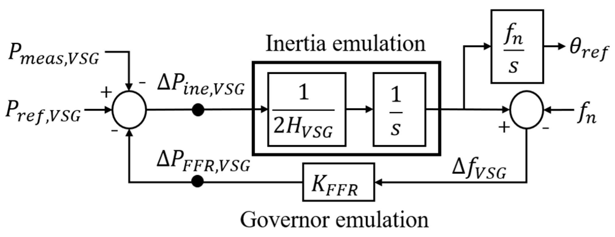
2.2. Definition of the EI of VSGs

In this section, we define the EI of VSGs in a system and describe the increase in the EI from the set inertia parameter using an active power control equation considering the SG swing equation, as shown in (1). The FFR of VSGs can increase their output in the inertia-time domain, increasing the EI of the VSGs.

By extending the aggregated SG and physical inertia formulation in (4), we add an extra term in (7) to represent the potential contribution of the EI $H_{EI}$ from non-SG generators (i.e., VSGs or other inverter-based resources).

$$M_{sys}=2H_{SG}^{ave}\sum _{i=1}^N{S}_{S{G}_i}+2H_{EI}\sum _{j=1}^L{S}_{E{I}_j},$$

(7)

where $S_{EI,j}$ is the capacity of the $j$-th generator excluding the SGs, and $L$ is the total number of generators for the EI calculation. Note that the EI is the average inertia of the generators, excluding the SGs. The EI $H_{EI}$ satisfies (3)–(6) and the physical inertia of the SGs $H_{SG}$ from the definition in (7). Therefore, this EI implies a contribution to the ROCOF via the physical inertia of the SGs and can be backcalculated from the ROCOF result of the time-domain simulation if the physical inertia $H_{SG}$ is known.

Subsequently, we examine the relationship between the EI and set parameters in the active power control of the VSGs. This active power control comprises two blocks (Figure 3)—inertia and governor emulation blocks—used to emulate the dynamics of the SGs [33]. Although the SG governor has a delay, as shown in (2), the VSGs can emulate the FFR (the non-delay governor), which exhibits simple proportional control. Therefore, the active power equation of the VSGs is expressed as shown in (8) and (9).

$$2H_{VSG}{S}_{VSG}{\displaystyle \frac{d∆f_{VSG}}{dt}}+K_{FFR}{S}_{VSG}∆f_{VSG}=-{∆P}_{out,VSG},$$

(8)

$$∆P_{out, VSG}=P_{meas,VSG}-P_{ref,VSG},$$

(9)

where $H_{VSG}$ is the set inertia parameters of the VSG, $S_{VSG}$ is the VSG capacity, $∆f_{VSG}$ is the rotating frequency deviation of the VSG from the nominal frequency $f_n$, ${\theta }_{ref}$ is the reference value of the phase for the PWM control of the VSG, $K_{FFR}$ is the FFR gain of the VSG, $P_{meas,VSG}$ is the measured active power output of the VSG, and $P_{ref,VSG}$ is the active power reference value under nominal conditions.

When the governor function is ignored in the inertia-time domain, as mentioned above, (1) can be rewritten as (10).

$$2H_{SG}{S}_{SG}{\displaystyle \frac{d∆f_{SG}}{dt}}=-∆P_{out,SG}.$$

(10)

As with (3), the aggregated equation of the system with SGs and VSGs can be written as follows, considering (8) and (10).

$$\left(\sum _{i=1}^{N}2H_{S{G}_i}{S}_{S{G}_i}+\sum _{j=1}^{L}2H_{{VSG}_j}{S}_{VS{G}_j}\right){\displaystyle \frac{d{∆f}_{agg}}{dt}}+\left(\sum _{j=1}^L{K}_{FF{R}_j}{S}_{VS{G}_j}\right)∆f_{agg}=-∆P_{out}^{agg}$$

(11)

When $-∆P_{out}^{agg}$ and $M_{sys}$ are substituted into (6) using (7) and (11), respectively, the EI of the VSGs is defined as (12) by comparing both sides of the equation with (5). Note that $∆H_{FFR}$ is given by (13).

$$H_{E{I}_{VSG}}=H_{VSG}^{ave}+∆H_{FFR},$$

(12)

$$∆H_{FFR}={\displaystyle \frac{\sum _{j=1}^L{K}_{FFR,j}{S}_{VSG,j}}{\sum _{j=1}^L{S}_{VSG,j}}}·{\displaystyle \frac{∆f_{agg}}{2\frac{d∆f_{agg}}{dt}}},$$

(13)

where $H_{VSG}^{ave}$ is the averaged set inertia parameter of the VSGs, calculated as the averaged inertia constant of the SGs ($H_{SG}^{ave}$) using (5), and $∆H_{FFR}$ is the increment of the EI $H_{EI,VSG}$ from $H_{VSG}^{ave}$ resulting from the FFR output.

From (12), we see that the EI of the VSG, $H_{E{I}_{VSG}}$, consists of two parts: (i) the averaged set inertia parameter $H_{VSG}^{ave}$, analogous to the physical inertia $H_{SG}^{ave}$, and (ii) $∆H_{FFR}$, the additional term arising from the FFR gain $K_{FFR}$ and the system frequency deviation. Physically, $∆H_{FFR}$ reflects the ability of the VSG to inject active power more rapidly than a conventional SG’s governor. Specifically, as described in (13), the increased $∆H_{FFR}$ is proportional to the product of the FFR gain $K_{FFR}$ and the deviation of the frequency variation. In the case of the ROCOF calculation in the infinitesimal time window of the inertia-time domain, $∆f_{agg}$ should not be zero. Thus, the EI of the VSGs increases from the set inertia parameter.

Note that the frequency variation after the disturbance, denoted as $∆f_{agg}$, is influenced by the active power dynamics between the generators. Equations (12) and (13) are related to the EI in terms of frequency. Conversely, these equations can be transformed into the active power. First, we divide the active power output of the generators into an inertia response, governor response, or FFR. The inertia of the SG and governor responses are defined in (14) and (15), respectively.

$$∆P_{ine,SG}=-2H_{SG}{S}_{SG}{\displaystyle \frac{d{∆f}_{SG}}{dt}},$$

(14)

$$∆P_{gov,SG}=-g\left(t, K_{SG}, T_{SG},S_{SG}, ∆f_{SG}\right),$$

(15)

where $g$ is the function resulting from solving the differential equation of (2) for $∆P_{in,SG}$. Note that $∆P_{gov,SG}$ has the same meaning as $∆P_{in,SG}$ in this study. Similar to those of the SG, from (8), the VSG inertia response and FFR are defined by (16) and (17), respectively.

$$∆P_{ine,VSG}=-2H_{VSG}{S}_{VSG}{\displaystyle \frac{d{∆f}_{VSG}}{dt}},$$

(16)

$$∆P_{FFR,VSG}=-K_{FFR}{S}_{VSG}∆f_{VSG}.$$

(17)

From (11) and (14)–(17), the active power relationship equation is obtained as in (18).

$$\sum _{i=1}^N∆P_{ine,S{G}_i}+\sum _{j=1}^L∆P_{ine,VS{G}_j}=∆P_{out}^{agg}-\sum _{j=1}^L∆P_{FFR,VS{G}_j},$$

(18)

Conversely, the equation of the system with only SGs can be described as in (19), considering (3) and (10).

$$\sum _{i=1}^N∆P_{ine,S{G}_i}=∆P_{out}^{agg}.$$

(19)

The difference between (18) and (19) represents the increase in the EI from the set inertia parameter of the VSGs. Equation (19) indicates that in an SG-only system, the entire disturbance $∆P_{out}^{agg}$ must be compensated by the physical inertia response of the SGs in the inertia-time domain. This leads directly to the ROCOF relationship shown in (6). However, in (18), we see that in a system containing VSGs, some portion of $∆P_{out}^{agg}$ can be offset by the FFR term $\sum _{j=1}^L∆P_{FFR,VS{G}_j}$ thereby reducing the net power imbalance that the inertia terms need to cover. As a result, the effective inertia from the VSG side appears larger than the set parameter, as the ROCOF will be lower than if FFR were absent.

Although the difference between the EI and set inertia parameter is described in terms of frequency, as shown in (13), the active power dynamics also affect the EI value, as described in (18). Using (11) and (14)–(17), the frequency deviation and derivative are described by (20) and (21), respectively.

$$∆f_{agg}=-{\displaystyle \frac{∆P_{out}^{agg}-\sum _{i=1}^N∆P_{ine,S{G}_i}-\sum _{j=1}^L∆P_{ine,VS{G}_j}}{\sum _{j=1}^L{K}_{FFR,j}{S}_{VSG,j}}}.$$

(20)

$${\displaystyle \frac{∆f_{agg}}{dt}}=-{\displaystyle \frac{∆P_{out}^{agg}-\sum _{j=1}^L∆P_{FFR,VS{G}_j}}{2H_{SG}^{ave}\sum _{i=1}^N{S}_{S{G}_i}+2H_{VSG}^{ave}\sum _{j=1}^L{S}_{VSG,j}}}.$$

(21)

As shown in (20) and (21), the frequency deviation $∆f_{agg}$ and its derivative are functions of the overall active power exchange among SGs and VSGs. Consequently, the EI of VSGs depends not only on the set inertia parameter and the FFR gain but also on the active power dynamics between the SGs and VSGs, the capacity ratio, and the set parameters of the VSGs. Because these factors collectively influence the EI, the next section examines each in detail and demonstrates how they affect the system’s response.

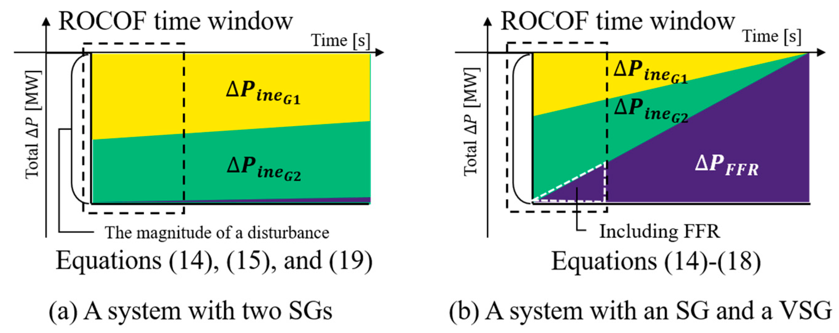
3. Factors Affecting the EI

In this section, we identify the factors that can affect the EI of VSGs. As explained in Section 2, these factors include active power dynamics, set parameters in the active power control system, the VSG’s inertia parameter $H_{VSG}$, FFR gain $K_{FFR}$, and VSG capacity ratio in the power system.

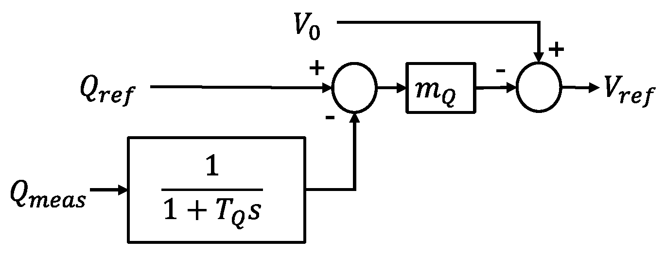
3.1. Effect of Set Parameters on VSGs

First, the set inertia parameter $H_{VSG}$ can affect the EI value of VSGs. The set inertia parameter determines the relationship between the active power deviation and derivative of the rotating frequency (Figure 3). This parameter emulates the physical inertia of SGs in the dynamics of VSGs. From (12), the EI of VSGs can be assumed to be proportional to the set inertia, and the coefficient can be 1.0. Conversely, the FFR gain determines the relationship between the active power and rotating frequency deviations. This emulates the governor dynamics of SGs without mechanical delays. According to (13), increasing $K_{FFR}$ can raise a VSG’s EI.

However, the increment $∆H_{FFR}$ caused by the FFR may also be affected by the FFR gain, set inertia parameter, and active power dynamics, as described in (20) and (21). This means that adjusting the set parameters of VSGs alters the rate of change in EI. A case study in Section 5 evaluates the sensitivities of these parameters.

3.2. Effect of the VSG Capacity Ratio

As described in (20) and (21), the EI can be affected by the generator capacity. In addition, both inertia response and FFR—key contributors to EI—can vary with generator capacity.

The EI of an SG remains unaffected by its capacity ratio, since all active power fluctuations are compensated by its physical inertia. By comparing (4) and (7), we see that the EI of an SG equals its physical inertia. In contrast, the EI of a VSG, as defined by (13), (20), and (21), depends on the generator capacity. Because EI is expressed on a per-unit basis (like physical inertia), the capacity ratio of a VSG significantly impacts its EI. Thus, understanding this dependence is crucial for designing VSGs in a power system.

Two VSG components vary with its capacity ratio changes: the interaction of active power responses in the system and the impedance from the point of disturbance. As described in (14)–(17), when the generator capacity varies, each term on the left-hand side of these equations also changes, altering the post-disturbance responses—including FFR—and thus affecting the EI in accordance with (13), (20), and (21).

Additionally, changing the VSG’s capacity ratio can vary the total impedance from the disturbance point to the VSGs. Because VSGs include filters and transformers, their total impedance often shifts alongside capacity adjustments. These impedance changes alter how the initial load is shared among generators after a disturbance, governed by the synchronizing power coefficient in (22).

$$SP{C}_{G_k}={\displaystyle \frac{E_{G_k}{V}_{dis}}{X_{G_k}}}cos{\delta }_{G_k},$$

(22)

where $SP{C}_{G_k}$ is the synchronizing power coefficient of the $k$-th generator of type $G$, which can be either an SG or VSG type, $E_{G_k}$ is the terminal voltage of $G_k$, $V_{dis}$ is the voltage at the disturbance point, $X_{G_k}$ is the total reactance from $G_k$ to the disturbance point, and ${\delta }_{G_k}$ is the phase difference from $G_k$ to the disturbance point. If $E_{G_k}$ and $cos{\delta }_{G_k}$ are assumed to be almost the same at each generator, the initial sharing ratio will depend on the reactance $X_{G_k}$. Therefore, the first active power variation of generator $G_k$, $∆P_{first,G_k}$, is expressed as (23).

$$∆P_{first,G_k}\cong {\displaystyle \frac{\frac{1}{X_{G_k}}}{{\sum }_{i=1}^p\frac{1}{X_{G_i}}}}∆P_{Load},$$

(23)

where p denotes the total number of generators in the system. Subsequently, changes in the VSG capacity ratio within the system alter the initial sharing ratio of the disturbance. This alteration influences the interaction of active power responses, as described in (20) and (21). However, this effect is not explicitly accounted for in the EI equations, as they do not model synchronizing power coefficients. To address this limitation, we analyzed the impact of the initial sharing ratio on the EI of the VSG in the case study presented in Section 5.

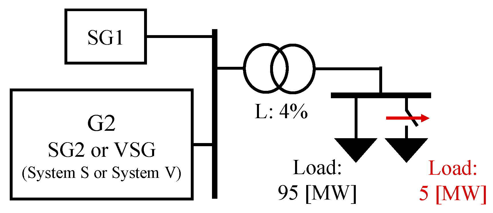
4. Case Study Simulation Settings

This section presents the simulation settings for case studies aimed at verifying the differences between the set inertia parameter on a VSG and the EI in terms of the factors described in Section 3. The EI of the VSG was computed using a simple system to analyze these factors and the outputs from the SG and VSG in detail. Subsequently, the EI calculation procedure, case settings, and analysis method for the simulation are described.

4.1. Simulation Model

To analyze the EI of the VSGs in a power system with SGs, we used a simple system that included SG1, G2 (SG2 or VSG), and a load, as shown in Figure 4. When G2 is SG2, the system is called System S. When G2 is a VSG, the system is called System V. The SG was modeled with two damping windings on the q-axis equivalent circuit in PSCAD/EMTDC [34]. The governor model of the SG is the first-lag model described in (3). The time constant $T_{SG}$ was 1.0 s, chosen to distinguish the governor’s slower response from the VSG’s fast-acting FFR within the 0.1 s inertia-time domain. The excitation controller model is based on a previous study [30]. A load trip of 5 MW was assumed to be the disturbance, and the magnitude of the disturbance was 5% of the system capacity, a common ratio used when evaluating frequency stability related to the governor output limitation [35]. The load was assumed to be a constant power for active and reactive powers.

The inverter-based resource was modeled as an averaged model; these references of the voltage magnitude and phase angle were derived from the controller (Figure 5) [36,37]. The output of the power calculator was obtained using the meter component in PSCAD/EMTDC. The following sections detail the parameters of the active power controller, while the reactive power control remained consistent across all cases, as depicted in Figure 6 [33]. The droop gain $m_Q$ was 0.1, and the time constant of the low-pass filter $T_Q$ was 0.08 s [33]. Note that in the modeling of VSG, although a single-loop average model is used, components that also exist in actual equipment, such as filters and step-up transformers, are simulated [11].

4.2. EI Calculation Procedure

This section describes the EI calculation procedure in this simulation based on the EI definition examined in Section 2.

For the EI calculation, we redefined the aggregated frequency $f_{agg}$ in (3) as the center of inertia (COI) frequency $f_{COI}$ as follows:

$$f_{COI}\left(t\right)={\displaystyle \frac{{\sum }_{i=1}^{p}2H_i{S}_i{f}_i\left(t\right)}{{\sum }_{k=1}^{p}2H_i{S}_i}},$$

(24)

where $H_i$ is the physical inertia or set inertia parameter of the $i$-th generator, $S_i$ is the $i$-th generator capacity, and $f_i\left(t\right)$ is the rotating frequency of the $i$-th generator. The COI frequency does not include the eigenoscillations of the rotating frequency of the SGs or VSGs. Therefore, the COI frequency represents the entire system frequency as the aggregated generator rotational frequency.

The EI was calculated as a metric describing the contribution of the COI frequency to the ROCOF. The ROCOF in the inertia-time domain is defined in (25).

$$ROCOF={\displaystyle \frac{f_{COI}\left(t_{dis}+∆t\right)-f_{COI}\left(t_{dis}\right)}{∆t}},$$

(25)

where $t_{dis}$ is the time of disturbance occurrence, and $∆t$ is the time window for calculating the ROCOF in the inertia-time domain.

In this study, the inertia-time domain was defined as 0.1 s, although some time windows were measured for system protection [3]. Therefore, $∆t$ was 0.1 s.

From (4)–(7), the EI of the VSG was calculated from (26).

$$H_{P{I}_{VSG}}={\displaystyle \frac{∆P_{Load}/\left(ROCOF\right(S_{SG}+S_{VSG}\left)\right)-2H_{SG}{r}_{SG}}{2r_{VSG}}},$$

(26)

where $r_{SG}$ and $r_{VSG}$ are the capacity ratios of the SG and VSG for the EI calculation, respectively.

4.3. Active Power Variation Evaluation Method

This section outlines the evaluation method for the EI of a VSG in terms of active power variation. The divided responses described in (14)–(17) were used for this analysis. These responses are visualized in a manner similar to Figure 2, enabling both qualitative and quantitative evaluations, as demonstrated in [38]. Additionally, the EI was calculated based on these responses to compare active power variations in a system containing only SGs with one containing both SGs and VSGs.

First, we describe the computation method for the active power variation $∆P$ in this study for each response, as outlined in (14)–(17). Each response was averaged over an inertia-time domain of 0.1 s as follows:

$$∆P_{R,G}^{ave}={\displaystyle \frac{\sum _{t=t_{start}}^{t_{start}+∆t_P}∆P_G\left(t\right)\times T_{step}}{∆t_P}},$$

(27)

where $R$ is the index of the type of response in the active power output of a type $G$ generator, $∆P_{R,G}^{ave}$ is the averaged type $R$ response of the type $G$ generator, $t_{start}$ is the start time of the calculation, $∆t_P$ is the time window of the active power variation, and $T_{step}$ is the time step of the simulation, set at 50 μs. Type R includes the inertia response of the SG and VSG, the governor response of the SG, and the FFR of the VSG. Each response was averaged because we calculated the ROCOF value in the time window of 0.05 s using (25). Note that these responses were computed in the EMT simulation of this study, as mentioned in Appendix A. Moreover, $t_{start}$ was 50.05 s after the disturbance, with $∆t_P$ at 0.05 s, because the load trip happened at 50 s, and an observation delay of the responses was present in the EMT simulation.

Subsequently, active power responses were analyzed to confirm that the FFR of VSGs contributes to differences between the EI and the set inertia parameter. EIs calculated from various combinations of responses were compared to those derived from the load trip magnitude, $H_{PIC}^{∆P_{Load}}$, equal to the EIs calculated from the ROCOF in Section 2.2. Two additional types of EI were defined for this analysis: the EI from the inertia responses $H_{PIC}^{∆P_{ine}}$ and the EI from all responses $H_{PIC}^{∆P_{all}}$. $∆P_{ine}$ in (28) was substituted for $∆P_{Load}$ in (26), and $∆P_{all}$, as described in (29), was substituted for $∆P_{Load}$ in (26).

$$∆P_{ine}=∆P_{ine,SG}+∆P_{ine,VSG},$$

(28)

$$∆P_{all}=∆P_{ine,SG}+∆P_{ine,VSG}+∆P_{gov,SG}+∆P_{FFR,VSG}.$$

(29)

From these calculations and comparisons, the influence of FFR on the increase in EI beyond the set inertia parameter was verified, as reflected in the differences between (18) and (19).

4.4. Case Settings

This section outlines the case settings for analyzing the EI characteristics of the VSG examined in Section 3. Three studies were conducted: an analysis of the difference between the set inertia constant and EI of the VSG (Study 1); a sensitivity analysis of the set parameters of the active power control (Study 2); and a sensitivity analysis of the VSG capacity ratio in the system (Study 3).

Table 1. Changed and fixed parameters in the sensitivity analysis studies.

Study #	Varied Parameters	Fixed Parameters
Study 2	VSG parameters $H_{VSG}$$\mathrm{and} K_{FFR}$	G2 ratio (50%)
Study 3	G2 ratio	Generator parameters (Table 2)

lists the variables and fixed parameters used in the sensitivity analysis studies.

Table 2. Generator parameters related to active power dynamics in the case studies.

System	Generator	$\mathit{H}$ [s]	$\mathit{K}$ [p.u.]	$\mathit{T}$ [s]
System S $(H=3$)	SG1	3.0	50	1.0
	SG2	3.0	50	1.0
System V $(H=3$)	SG1	3.0	50	1.0
	VSG	3.0	50	-
System S $(H=6$)	SG1	3.0	50	1.0
	SG2	6.0	50	1.0
System V $(H=6$)	SG1	3.0	50	1.0
	VSG	6.0	50	-

lists the fixed parameters for each generator shown in Figure 4: the set inertia parameter is chosen to represent standard thermal generators [35], and the governor and FFR gains are selected within stable EMT simulation limits near typical practical values. Note that all of these parameters are relevant to active power dynamics, as evident from (1), (2), and (8).

Study 1 examined the difference between the set inertia constant and the EI of the VSG by comparing the active power outputs of Systems S and V (Figure 4). As noted in Section 2.1, the EI of synchronous generators (SGs) is identical to their physical inertia, whereas the EI of VSGs exceeds their set inertia parameter. This comparison aims to identify the cause of this discrepancy. The EIs and active power outputs of the SG and VSG were compared for $H=3$ and $H=6$ to investigate the effect of the FFR on the EI with different set inertia parameters. After simulating a load trip, the EIs of the VSG and SG2 were calculated. The differences between these values were analyzed in terms of inertia, governor responses, and FFR.

Study 2 analyzed the sensitivity of the set parameters in the VSG active power control block to the EI of the VSG in System V. The EI sensitivity was evaluated in terms of the set inertia parameter and FFR gain. The sensitivity was evaluated by varying the set inertia parameter $H_{VSG}$ from 3 s to 20 s with several fixed FFR gains. Additionally, the FFR gain $K_{FFR}$ was varied from 50 to 500 with several fixed set inertia parameters. The sensitivity analysis utilized the EI Equations (12) and (13), considering active power responses.

Study 3 examined the sensitivity of the VSG capacity ratio to the EI in Systems S and V. As discussed in Section 3.2, changes in the VSG capacity ratio affect the initial sharing ratio of the disturbance. The EI sensitivity was analyzed by evaluating changes in each response related to the initial sharing ratio. In Systems S and V, the G2 ratio was varied from 10% to 90% in 1% increments.

5. Results and Analysis

In this section, the frequency and EI calculation results are analyzed with respect to the active power responses of the SG and VSG. We analyzed the EI through three studies, as mentioned in Section 4.4.

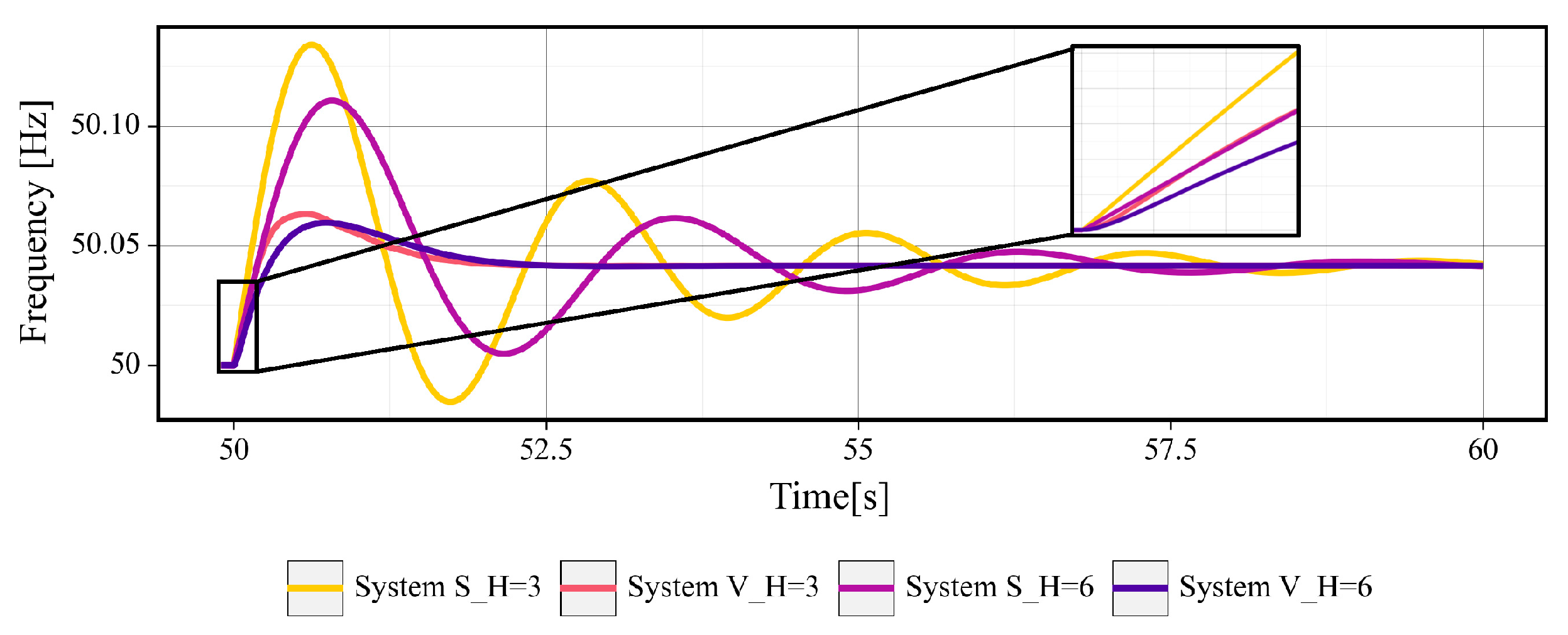
5.1. Larger EI than the Set Inertia Parameter (Study 1)

In this section, we analyze the effect of the FFR of the VSG on the EI. Under identical physical and set inertia parameters, the SG-VSG hybrid system showed greater stability because its FFR acted within the inertia-time domain, supplementing the inertia response. The detailed results are explained as follows.

Figure 7 shows the simulation results of the COI frequency variation after the load trip in Study 1. Note that the load trip occurred at 50 s in the EMT simulation. We compared SG2 and the VSG with the same physical inertia $H_{SG}$ and set inertia parameter $H_{VSG}$ for $H=3$ and $H=6$, respectively. Despite identical parameters, the ROCOF of the COI frequency of System V was smaller than that of System S, as summarized in Table 2. Comparing System S and System V for the other values revealed that System V had a smaller peak value and an earlier peak position with fewer oscillations. This behavior occurred because VSG’s FFR had no delay, unlike the SG governor, thus improving frequency stabilization. Ten seconds after the disturbance shown in Figure 7, all frequency variations converged to the same frequency value because the value of the FFR gain $K_{FFR}$ equaled the governor gain of the SG $K_{SG}$. This result indicates that the VSG contributes more to the ROCOF reduction than the SG.

Figure 8 presents the EIs calculated using the method described in Section 4.2. The EI of the SG matched its physical inertia $H_{SG}$, while the EI of the VSG exceeded its set inertia parameter $H_{VSG}$ for both $H=3$ and $H=6$. This result was consistent with the ROCOF results. Specifically, the EI increased by 96% for $H=3$ and by 58% for $H=6$, consistent with the ROCOF results.

To understand the EI increase in the VSG beyond its set inertia parameter $H_{VSG}$, we analyzed the active power responses of each generator based on their responses, as described in Section 3 and Section 4. Figure 9 shows the accumulation of the active power responses after the load trip. The magnitude of the load trip $∆P_{load}$ = 5.0 MW is shared by the two responses of each generator in each system. Each response is defined by (14)–(17) and measured within the EMT simulation. Appendix A details the measurement method for both SG and VSG. Figure 9a,c depict the responses in System S, while Figure 9b,d show those in System V. Measurement differences in the EMT simulation caused a delay in the observed responses, as the VSG outputs were directly measured from the control block, bypassing the hidden filter in PSCAD/EMTDC. Thus, responses were calculated within the time window of 0.05–0.1 s, as described in Section 4.3.

As shown in Figure 9a,b, the FFR of the VSG compensated for the load trip more rapidly than the SG’s governor response, which was slowed by mechanical delays. These differences were also observed for $H=6$, as shown in Figure 9c,d, and they aligned with the EI results derived from active power responses, as explained in Section 4.3.

Table 3. Values of each metric in Study 1. Metric $H_{PIC}^{∆P_{ine}}$ remains close to the set inertia parameter, while $H_{PIC}^{∆P_{all}}$ exceeds it. This suggests that FFR causes an increase in EI beyond the set inertia parameter from the viewpoint of active power.

Metrics	System S (H = 3)	System V (H = 3)	System S (H = 6)	System V (H = 6)
ROCOF [Hz/s]	0.340	0.231	0.228	0.164
EI of G2 $H_{PIC}^{∆P_{load}}$ [s]	3.00	5.88	6.00	9.48
EI of G2 $H_{PIC}^{∆P_{ine}}$ [s]	3.05	2.97	6.06	7.29
EI of G2 $H_{PIC}^{∆P_{all}}$ [s]	2.98	5.75	6.15	8.98

lists the ROCOFs and EIs calculated using the methods described in Section 4.3. The EIs derived from inertia responses $H_{PIC}^{∆P_{ine}}$ closely matched the set inertia parameter of the VSG, confirming the accuracy of its inertia emulation. In contrast, the EIs from all responses $H_{PIC}^{∆P_{all}}$ were larger than the set inertia constant of the VSG and exhibited trends similar to those derived from the load trip magnitude $H_{PIC}^{∆P_{load}}$. This increase was attributed to the FFR of the VSG, as the SG governor did not respond within 0.1 s after the disturbance. The discrepancy between $H_{PIC}^{∆P_{all}}$ and $H_{PIC}^{∆P_{load}}$ arose from limitations in the active power calculation time window. Although these limitations highlight the need for improved measurement methods, the analysis clearly demonstrated that the increase in EI from the set inertia parameter is due to the contributions of the VSG’s FFR.

5.2. EI Sensitivity Analysis of the Set Parameters (Study 2)

This section presents the sensitivity analysis of the set of parameters of the VSG considering the EI of the VSG. As mentioned in Section 3.1, the EI depends on the set inertia parameter $H_{VSG}$ and the FFR gain $K_{FFR}$ in the VSG active power control. Theoretically, as described in (12) and (13), the EI should be proportional to each parameter.

First, the EI sensitivity of $H_{VSG}$ was analyzed. Figure 10 shows the variation in EI with $H_{VSG}$ for several FFR gains. The EI increased almost linearly for all FFR gains. According to (12), EI is expressed as a linear function of $H_{VSG}^{ave}$ with a coefficient of 1.0 if we ignore the other terms included in (13) regarding $H_{VSG}^{ave}$. However, the average value of the five coefficients considered in this equation obtained using the least-squares method was 1.24. This difference of 0.24 can be attributed to the active power dynamics between the SG and VSG, as shown in (20) and (21).

Figure 11 shows the active power deviation of the inertia responses of the SG, VSG, and FFR of the VSG for each sensitivity analysis case determined using (27). As $H_{VSG}$ increased, the inertia response of the VSG increased, while its FFR decreased. The inertia response of the SG also decreased despite its physical inertia remaining unchanged. This reduction in the SG’s inertia response effectively increased the VSG’s total response, leading to a coefficient greater than 1.0.

Subsequently, the EI sensitivity of the FFR gain was analyzed. Figure 12 shows that the EI varied nearly linearly in all cases of $K_{FFR}$. The average value of the five coefficients from each line in Figure 12 is 0.02, significantly smaller than the coefficient of the set inertia parameter of 1.24. Figure 13 shows the active power deviation of the three responses for the sensitivity analysis of the FFR gain. Compared with the $H_{VSG}$ sensitivity results, the VSG’s FFR response in Figure 13 shows a greater variation, while its inertia response also changes more substantially. However, the total response of the VSG did not vary as significantly as it did in the $H_{VSG}$ sensitivity analysis. This explains why the EI sensitivity coefficient for the FFR gain was significantly lower than that of $H_{VSG}$. Although $H_{VSG}$ has a more significant impact on the EI of the VSG, power system operators should consider the FFR gain setting when addressing frequency stability issues.

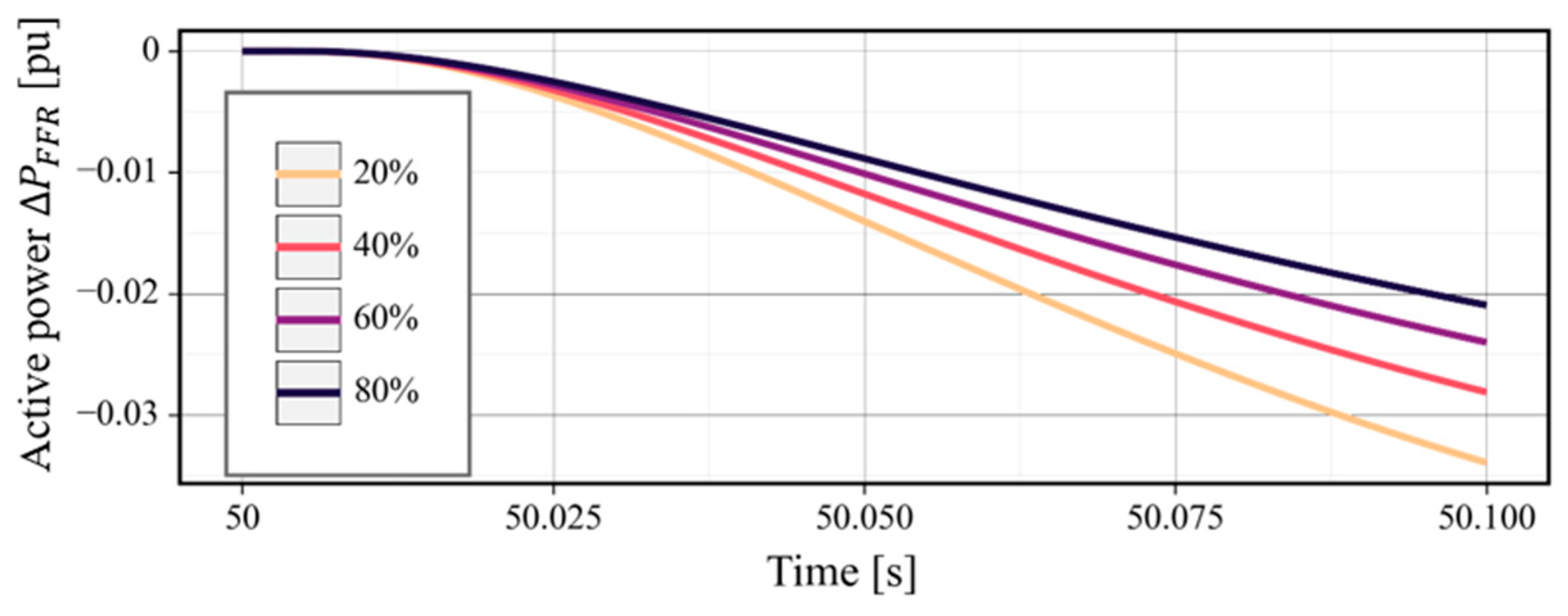
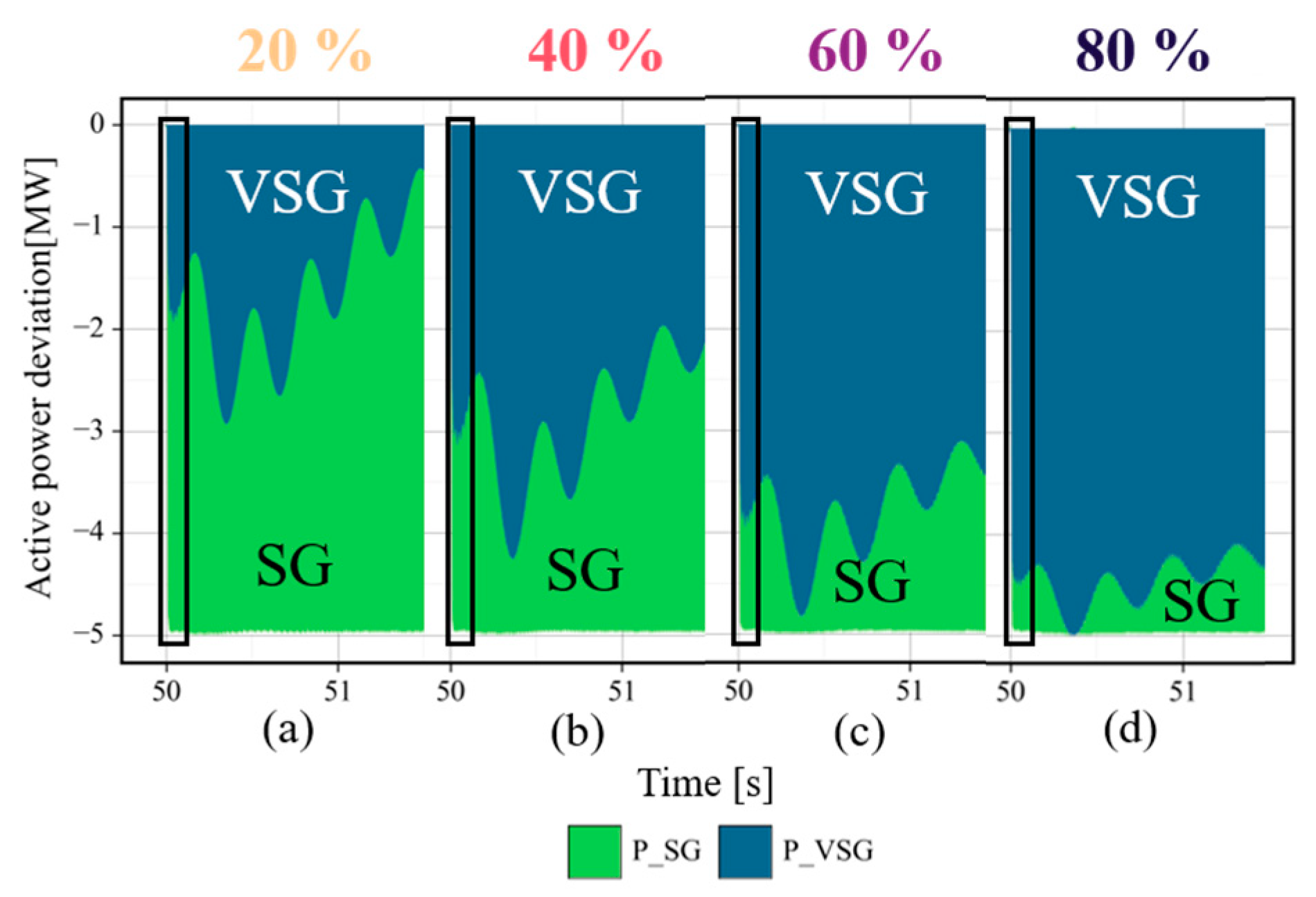
5.3. EI Sensitivity Analysis of the Capacity Ratio (Study 3)

This section presents a sensitivity analysis of the capacity ratio of the VSG to its EI. As mentioned in Section 3.2, the EI depends on the capacity ratio due to changes in the initial sharing ratio and the response of each system after a disturbance. The set parameters of the VSG were fixed, as listed in Table 2.

First, we examined the dependence of the ROCOF results on the G2 capacity ratio. Figure 14 shows that the frequency variation changed with the G2 ratio for System V with $H=3$. Figure 15a shows the variation in the ROCOF with the G2 ratio for each system. In System S with $H=3$, the ROCOFs were constant because the physical inertia $H_{SG}$ of SG2 matched that of SG1 (Table 2). The ROCOFs of the other systems decreased as the G2 ratio increased because the EI value of each G2 unit exceeded $H_{SG}$ of the SG1.

Subsequently, we examined the EIs of G2, calculated based on the G2 capacity ratio. Figure 15b shows the relationship between the G2 capacity ratio and EIs of SG2 and the VSG in each system derived from the ROCOFs shown in Figure 15a. The EIs of SGs remained constant across all G2 ratios, consistent with the SG physical inertia theory described in Section 2.1, validating the EI calculations. In contrast, the EIs of the VSG decreased as the G2 ratio increased. Notably, the decline in EI was more pronounced when the VSG ratio was small. This dependency on the VSG ratio presents a challenge for system operators managing VSGs based on EI. To address this, we analyzed the causes of the VSG EI dependence on the capacity ratio.

The EI dependence on the VSG ratio is influenced by the FFRs of each VSG unit. Figure 16 shows the FFR variation of the VSG in $H=3$ across different VSG ratios. When the VSG capacity ratio was low, the variation in the FFR increased, resulting in a small ROCOF and higher EI. These results highlight the EI dependence on the VSG capacity ratio.

Moreover, the decrease in FFR per unit as the VSG ratio increased is attributed to active power dynamics between SG1 and the VSG, as described in (20) and (21). Starting from the initial sharing ratio, a low initial sharing ratio limits the FFR output, leading to higher frequency variations and an increased per-unit FFR, as shown in (17). Consequently, the EI with a low initial sharing ratio is larger than that with a high initial sharing ratio.

Figure 17 illustrates the active power variations within 1.5 s of the load trip for different VSG ratios. Changes in the initial sharing ratio result from variations in the synchronizing power coefficients, which are influenced by the total reactance of each generator relative to the disturbance point, as described in (23). When the G2 ratio changed, the VSG filter and transformer capacities also changed, altering the total reactance $X_{VSG}$ of the VSG. Consequently, this variation in reactance influenced the synchronizing power coefficients and initial sharing ratios, thereby affecting the FFR and the calculated EI.

This paragraph summarizes the findings in this section and explains why increasing the VSG capacity ratio leads to a diminished rise in the VSG’s EI from its set inertia. We attribute these results to the larger VSG’s synchronizing power coefficients and initial sharing ratio associated with a larger VSG capacity ratio, primarily due to lower filter and transformer impedances, as in (23) and Figure 17. Consequently, the “total” FFR responds more quickly to a disturbance than it does under smaller synchronizing power coefficients and initial sharing ratio, thereby suppressing frequency variation. As illustrated in Figure 16, this results in a reduced “per-unit” FFR, which in turn limits the increase in the VSG’s EI above its set inertia parameter. Although previous work [22] has indicated that FFR contributes to the inertia-time domain and can increase the EI, it has not been discussed that the EI can also change due to the VSG capacity ratio and synchronizing power coefficients. This point represents the novelty of this study.

5.4. Toward Evaluating Effective Inertia in Real Power Systems

In this section, we discuss the practical challenges of implementing our study’s findings in real power systems. Our results indicate that FFR increases the VSG’s EI beyond its set inertia parameter (Section 5.1) and that the impact of FFR depends on the synchronizing power coefficients associated with the VSG capacity ratio (Section 5.3). The fundamental characteristics of the FFR effect, as analyzed in this study, will remain valid in real power systems, which supply electric power to wide areas with multiple synchronous and non-synchronous generators. Indeed, the performance of FFR is primarily determined by its gain, and our sensitivity analysis indicates that increasing this gain raises the EI (Section 5.2). However, how much the EI exceeds its set inertia will vary under real-world conditions, which affect the FFR response speed, VSG capacity ratio, and synchronizing power coefficients of each generator, although the basis of our findings holds universally.

There are three major concerns when applying our findings to real-world conditions. The first is the inherent uncertainty and variability in real power systems—for example, hybrid systems that include various types of SGs and IBRs, as well as parameter deviations, noise, and fluctuating grid conditions. These are not fully captured in the simple-modeled power system used in this study. Under such circumstances, the EI of VSGs can change due to variations in the synchronizing power coefficients related to the VSG capacity ratio as discussed in Section 5.3, caused by the dynamic connection status of generators.

The second concern is real-time implementation feasibility and economic considerations. Cost-effectiveness is important in power system operations, and accounting for EI can help avoid unnecessary generation. However, more flexible EI modeling is needed to accommodate diverse real-time and market conditions.

The third concern involves the hardware implementation constraints of VSGs. In this study, we used a single-loop averaged model in the EMT simulations, which closely approximates real hardware [32]. However, in actual VSG implementation, additional functionalities may introduce control delays that reduce the VSG’s measured output. For instance, even in our simulation results, a delay in the measurement filter caused a reduction in the measured VSG output as shown in Figure 9, suggesting that a similar effect could occur in hardware devices. Therefore, integrating our findings with hardware testing would provide further clarity and precision.

In summary, although more complex and variable conditions may alter the FFR and EI behavior, the main conclusions of this paper should remain valid.

6. Conclusions

This study quantitatively analyzed the difference between the EI of a VSG and the set inertia parameters in an active power control system. The simulation results were analyzed by dividing the active power output of the VSG into the inertia responses of the SG and VSG, the governor response of the SG, and the FFR of the VSG.

The main findings of this study are summarized as follows:

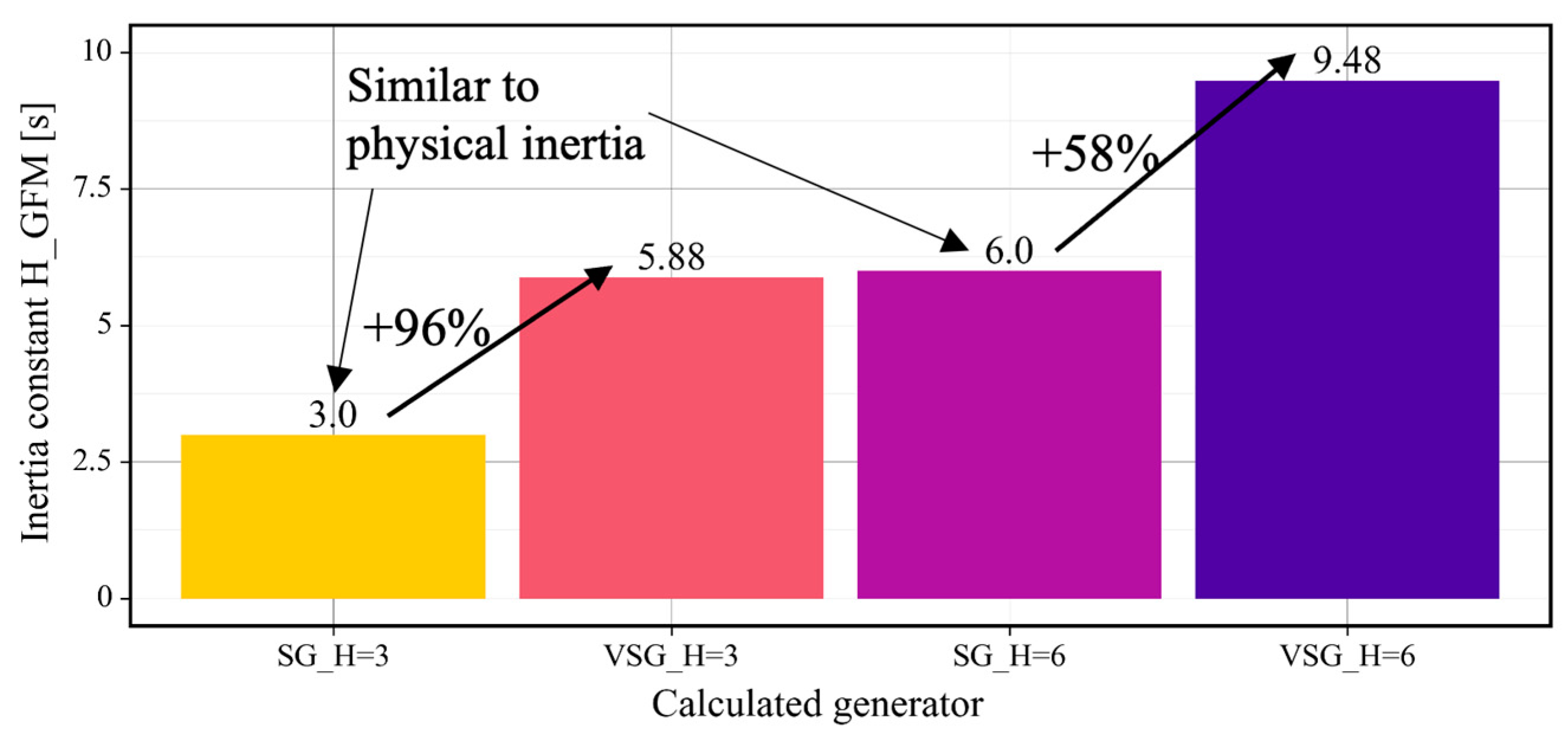
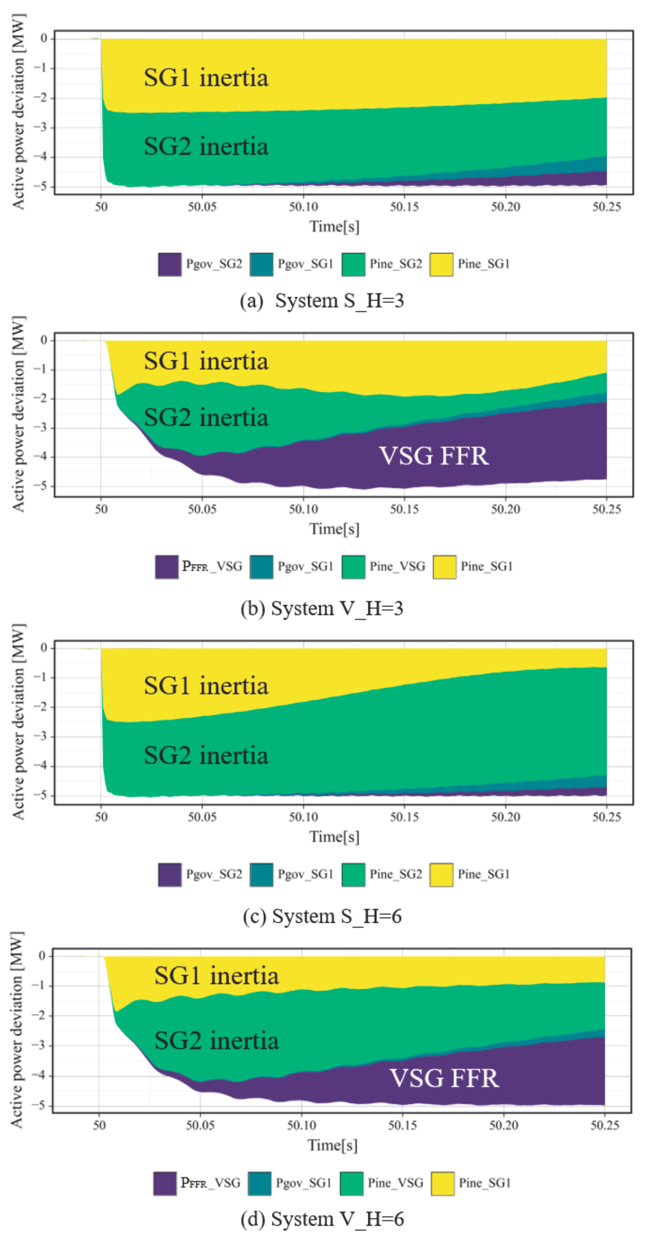
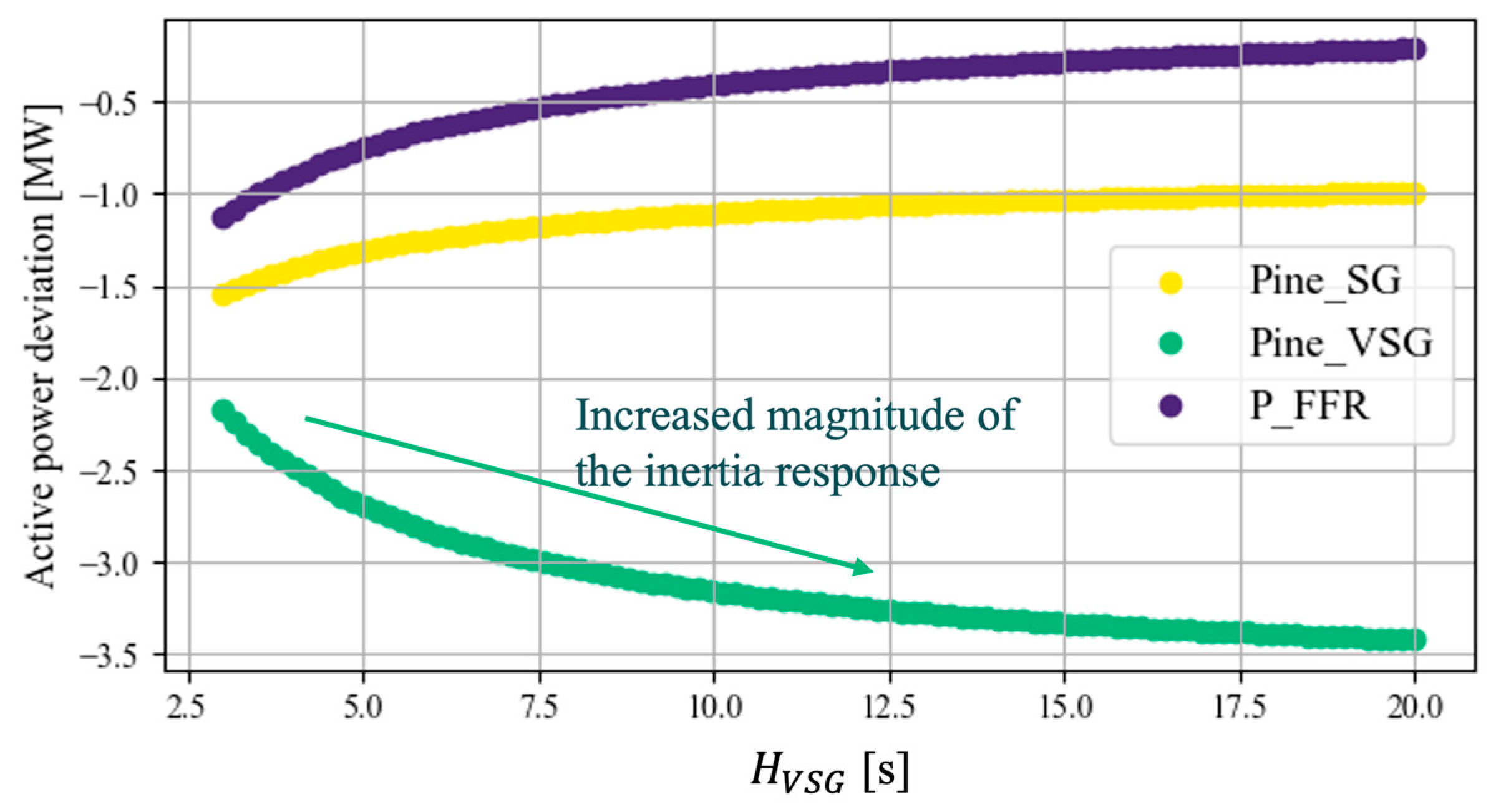
• After the disturbance in the inertia-time domain, the FFR of the VSG suppressed the inertia response of the SG, increasing the EI of the VSG beyond its set inertia parameter. The traditional method for analyzing the relationship between the physical inertia of SGs and the ROCOF does not consider the FFR. Under certain conditions, the EI of the VSG increased from the set inertia parameter by 96%.
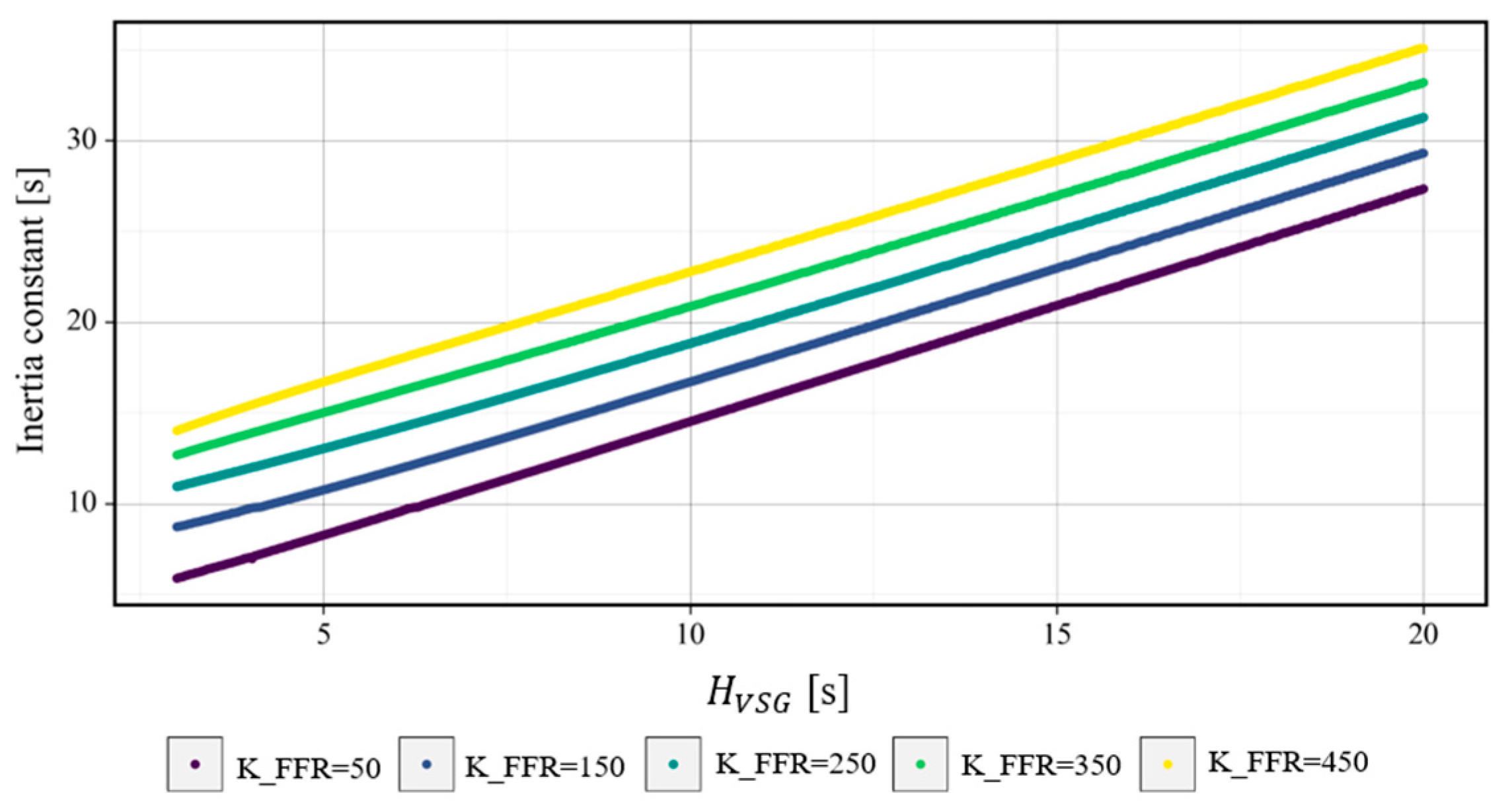
• The EI of the VSG varied nearly linearly with the set parameters of $H_{VSG}$ and $K_{FFR}$, with the sensitivity to $H_{VSG}$ being significantly higher than that to $K_{FFR}$. Nevertheless, both $H_{VSG}$ and $K_{FFR}$ were found to be crucial for EI assessment, as demonstrated by the notable impact of $K_{FFR}$ in the FFR sensitivity analysis.
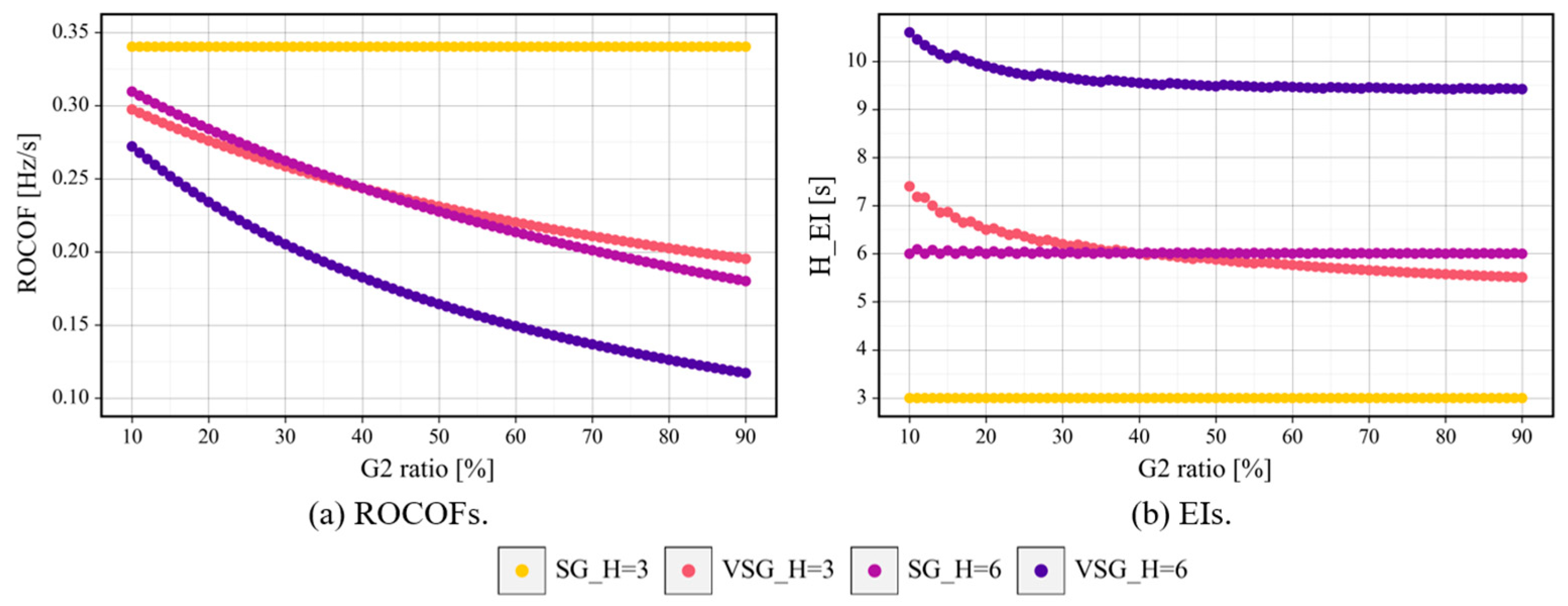
• The EI of the VSG decreased as the VSG’s capacity ratio increased relative to the total generation capacity. This resulted from the change in the per-unit FFR owing to the change in the synchronous power coefficients and initial sharing ratio between the generators immediately after the disturbance.

In this study, the EI was calculated for a simple system and analyzed in terms of this fundamental characteristic for the smooth introduction of VSG. Future studies could investigate EI using larger, more complex system configurations subject to load noise and voltage fluctuations as well as experimental setups with real hardware and communication systems to validate our simulations. Moreover, developing planning methods or real-time control strategies that exploit EI could enable more cost-effective unit commitment and dynamic operation. The detailed limitation, challenge, and future directions are described in Section 5.4.

References

1. Milano, F.; Dörfler, F.; Hug, G.; Hill, D.J.; Verbič, G. Foundations and challenges of low-inertia systems (invited paper). In Proceedings of the Power Systems Computation Conference (PSCC), Dublin, Ireland, 11–15 June 2018; pp. 1–25. [Google Scholar]
2. Hatziargyriou, N.; Milanovic, J.; Rahmann, C.; Ajjarapu, V.; Canizares, C.; Erlich, I.; Hill, D.; Hiskens, I.; Kamwa, I.; Pal, B.; et al. Definition and classification of power system stability—Revisited & extended. IEEE Trans. Power Syst. 2021, 36, 3271–3281. [Google Scholar]
3. Protection & Dyn. Sub Group. Frequency Measurement Requirements and Usage. Available online: https://eepublicdownloads.entsoe.eu/clean-documents/SOC%20documents/Regional_Groups_Continental_Europe/2018/TF_Freq_Meas_v7.pdf (accessed on 1 November 2023).
4. Driesen, J.; Visscher, K. Virtual synchronous generators. In Proceedings of the 2008 IEEE Power and Energy Society General Meeting, Pittsburgh, PA, USA, 20–24 July 2008; pp. 1–3. [Google Scholar]
5. Bevrani, H.; Ise, T.; Miura, Y. Virtual synchronous generators: A survey and new perspectives. Int. J. Electr. Power Energy Syst. 2014, 54, 244–254. [Google Scholar] [CrossRef]
6. Li, D.; Zhu, Q.; Lin, S.; Bian, X.Y. A self-adaptive inertia and damping combination control of VSG to support frequency stability. IEEE Trans. Energy Convers. 2017, 32, 397–398. [Google Scholar] [CrossRef]
7. Li, C.; Yang, Y.; Mijatovic, N.; Dragicevic, T. Frequency stability assessment of grid-Forming VSG in framework of MPME with feedforward decoupling control strategy. IEEE Trans. Ind. Electron. 2022, 69, 6903–6913. [Google Scholar] [CrossRef]
8. Hou, X.; Sun, Y.; Zhang, X.; Lu, J.; Wang, P.; Guerrero, J.M. Improvement of frequency regulation in VSG-based AC microgrid via adaptive virtual inertia. IEEE Trans. Power Electron. 2020, 35, 1589–1602. [Google Scholar] [CrossRef]
9. Yao, F.; Zhao, J.; Li, X.; Mao, L.; Qu, K. RBF neural network based virtual synchronous generator control with improved frequency stability. IEEE Trans. Ind. Inform. 2021, 17, 4014–4024. [Google Scholar] [CrossRef]
10. Fini, M.H.; Golshan, M.E.H. Determining optimal virtual inertia and frequency control parameters to preserve the frequency stability in islanded microgrids with high penetration of renewables. Electr. Power Syst. Res. 2018, 154, 13–22. [Google Scholar] [CrossRef]
11. Orihara, D.; Kikusato, H.; Hashimoto, J.; Otani, K.; Takamatsu, T.; Oozeki, T.; Taoka, H.; Matsuura, T.; Miyazaki, S.; Hamada, H.; et al. Contribution of voltage support function to virtual inertia control performance of inverter-based resource in frequency stability. Energies 2021, 14, 4220. [Google Scholar] [CrossRef]
12. Tayyebi, A.; Groß, D.; Anta, A.; Kupzog, F.; Dörfler, F. Frequency stability of synchronous machines and grid-forming power converters. IEEE J. Emerg. Sel. Top. Power Electron. 2022, 8, 1004–1018. [Google Scholar] [CrossRef]
13. Mohamad, A.M.E.I.; Mohamed, H.R.A.; Mohamed, Y.A.-R.I. Impedance-Based Stability Analysis of a Low-Inertia AC Grid Connected to a DC Grid by a VSC with Virtual Inertia Controllers. IEEE Open J. Power Electron. 2025, 1–18. [Google Scholar] [CrossRef]
14. Liu, J.; Miura, Y.; Ise, T. Comparison of dynamic characteristics between virtual synchronous generator and droop control in inverter-based distributed generators. IEEE Trans. Power Electron. 2016, 31, 3600–3611. [Google Scholar] [CrossRef]
15. Aragon, D.A.; Unamuno, E.; Ceballos, S.; Barrena, J.A. Comparative small-signal evaluation of advanced grid-forming control techniques. Electr. Power Syst. Res. 2022, 211, 108154. [Google Scholar] [CrossRef]
16. Luo, J.; Teng, F.; Bu, S. Stability-Constrained Power System Scheduling: A Review. IEEE Access 2020, 8, 219331–219343. [Google Scholar]
17. Tayyebi, A.; Dörfler, F.; Kupzog, F.; Miletic, Z.; Hribernik, W. Grid-forming converters-inevitability control strategies and challenges in future grids application. In Proceedings of the CIRED Workshop, Ljubljana, Slovenia, 7–8 June 2018. [Google Scholar]
18. Hirase, Y.; Sugimoto, K.; Sakimoto, K.; Ise, T. Analysis of resonance in microgrids and effects of system frequency stabilization using a virtual synchronous generator. IEEE J. Emerg. Sel. Top. Power Electron. 2016, 4, 1287–1298. [Google Scholar]
19. Tuttelberg, K.; Kilter, J.; Wilson, D.; Uhlen, K. Estimation of Power System Inertia from Ambient Wide Area Measurements. IEEE Trans. Power Syst. 2018, 33, 7249–7257. [Google Scholar]
20. Dhara, P.K.; Rather, Z.H.; Phurailatpam, C. Estimation of Minimum Inertia and Fast Frequency Support for Renewable Energy Dominated Power Systems. IEEE Trans. Instrum. Meas. 2025, 74, 1–14. [Google Scholar]
21. Ruan, Y.; Yao, W.; Zong, Q.; Zhou, H.; Gan, W.; Zhang, X.; Li, S.; Wen, J. Online Assessment of Frequency Support Capability of the DFIG-Based Wind Farm Using a Knowledge and Data-Driven Fusion Koopman Method. Appl. Energy 2025, 377, 124518. [Google Scholar]
22. Hua, W.; Li, D.; Mi, Y. Power System Inertia Estimation during Normal Operation Using Adaptive Ensemble Empirical Mode Decomposition. Electr. Power Syst. Res. 2025, 241, 111305. [Google Scholar] [CrossRef]
23. Im, S.; Park, J.; Lee, K.; Son, Y.; Lee, B. Estimation of Quantitative Inertia Requirement Based on Effective Inertia Using Historical Operation Data of South Korea Power System. Sustainability 2024, 16, 10555. [Google Scholar] [CrossRef]
24. Jiang, B.; Guo, C.; Chen, Z. Frequency Constrained Dispatch with Energy Reserve and Virtual Inertia from Wind Turbines. IEEE Trans. Sustain. Energy 2025, 16, 1340–1355. [Google Scholar]
25. Zhang, H.; Liao, K.; Yang, J.; Zheng, S.; He, Z. Frequency-Constrained Expansion Planning for Wind and Photovoltaic Power in Wind-Photovoltaic-Hydro-Thermal Multi-Power System. Appl. Energy 2024, 356, 122401. [Google Scholar]
26. Imgart, P.; Chen, P. Effective Inertia Constant: A Frequency-Strength Indicator For Converter-Dominated Power Grids. In Proceedings of the 2023 IEEE Belgrade PowerTech, Belgrade, Serbia, 25–28 June 2023; pp. 1–6. [Google Scholar]
27. Soni, N.; Doolla, S.; Chandorkar, M.C. Improvement of transient response in microgrids using virtual inertia. IEEE Trans. Power Deliv. 2013, 28, 1830–1838. [Google Scholar]
28. Shobug, M.A.; Chowdhury, N.; Hossain, M.A.; Sanjari, M.J.; Lu, J.; Yang, F. Virtual Inertia Control for Power Electronics-Integrated Power Systems: Challenges and Prospects. Energies 2024, 17, 2737. [Google Scholar] [CrossRef]
29. Sati, S.E.; Al-Durra, A.; Zeineldin, H.; EL-Fouly, T.H.M.; El-Saadany, E.F. A Novel Virtual Inertia-Based Damping Stabilizer for Frequency Control Enhancement for Islanded Microgrid. Int. J. Electr. Power Energy Syst. 2024, 155, 109580. [Google Scholar]
30. Norouzi, M.H.; Oshnoei, A.; Mohammadi-Ivatloo, B.; Abapour, M. Learning-Based Virtual Inertia Control of an Islanded Microgrid with High Participation of Renewable Energy Resources. IEEE Syst. J. 2024, 18, 786–795. [Google Scholar]
31. Gurski, E.; Kuiava, R.; Perez, F.; Benedito, R.A.S.; Damm, G. A Novel VSG with Adaptive Virtual Inertia and Adaptive Damping Coefficient to Improve Transient Frequency Response of Microgrids. Energies 2024, 17, 4370. [Google Scholar] [CrossRef]
32. Kundur, P. Power System Stability and Control; McGraw-Hill Education, Inc.: New York, NY, USA, 1994; pp. 581–582. [Google Scholar]
33. D’Arco, S.; Suul, J.A. Virtual synchronous machines—Classification of implementations and analysis of equivalence to droop controllers for microgrids. In Proceedings of the IEEE Grenoble Conference, Grenoble, France, 16–20 June 2013; pp. 1–7. [Google Scholar]
34. Anderson, P.M.; Fouad, A.A. Power System Control and Stability, 2nd ed.; IEEE Press: Piscataway, NJ, USA, 2003; pp. 13–52, 83–148. [Google Scholar]
35. Institution of Electrical Engineering in Japan. Japanese Power System Model. Available online: http://www.iee.or.jp/pes/model/english/ (accessed on 27 January 2025).
36. Rocabert, J.; Luna, A.; Blaabjerg, F.; Rodríguez, P. Control of power converters in AC microgrids. IEEE Trans. Power Electron. 2012, 27, 4734–4749. [Google Scholar]
37. Mo, O. Average Model of PWM Converter; Project Memo SINTEF/12X127.02; SINTEF: Trondheim, Norway, 2003; Available online: https://www.sintef.no/globalassets/project/powerelectronics/slideshow-an0312103.pdf (accessed on 27 January 2025).
38. Shikuma, R.; Orihara, D.; Kikusato, H.; Taoka, H.; Kaneko, A.; Hayashi, Y. Quantitative Effect of the Inertia Emulation Block of Grid-Forming Inverters on Frequency Stability. In Proceedings of the 2023 IEEE Belgrade PowerTech, Belgrade, Serbia, 25–28 June 2023; pp. 1–6. [Google Scholar]
Figure 1. Overview of the EI derivation process from the ROCOF for SGs and VSGs. A schematic illustrating the theoretical process of deriving the EI from the ROCOF in both conventional SG systems and SG-VSG hybrid systems.
Energies 18 01683 g001
Figure 2. Conceptual diagram of active power dynamics in (a) a system with two SGs and (b) a system with an SG and a VSG, illustrating how FFR affects the EI of the VSG by altering its active power output immediately after a disturbance.
Energies 18 01683 g002
Figure 3. Active power control of VSGs, comprising an inertia and FFR emulation block.
Energies 18 01683 g003
Figure 4. Case-study power system, comprising one synchronous generator (SG) and either an additional SG or a VSG.
Energies 18 01683 g004
Figure 5. IBR model for the VSG, comprising an averaged model, a transformer, and a filter.
Energies 18 01683 g005
Figure 6. Reactive power control of the VSG, comprising a filter and a proportional control block.
Energies 18 01683 g006
Figure 7. Frequency variations in each system, compared by the G2 inertia parameter.
Energies 18 01683 g007
Figure 8. Calculated EIs in each system, illustrating that VSGs exhibit values different from the set inertia parameter.
Energies 18 01683 g008
Figure 9. Accumulated responses after the disturbance: (a) SG2 ( H s g = 3 ) exhibits the same response as SG1. (b) The VSG provides FFR within 0.1 s. (c) SG2 ( H s g = 6 ) increases the inertia response beyond that of SG1. (d) The VSG provides a larger inertia response than in (a).
Energies 18 01683 g009
Figure 10. EI variations with changes in the set inertia parameter, demonstrating a similar ratio of change for each FFR gain.
Energies 18 01683 g010
Figure 11. Relationship between the set inertia parameter and the generator responses, showing that the higher set inertia parameter results in the larger inertia response of the VSG.
Energies 18 01683 g011
Figure 12. EI variations with changes in the FFR gain, demonstrating a similar ratio of change for each set inertia parameter.
Energies 18 01683 g012
Figure 13. Relationship between the FFR gain and the generator responses, showing that the higher FFR gain results in the larger FFR of the VSG.
Energies 18 01683 g013
Figure 14. Frequency variations in System V of H = 3 at different VSG ratios, showing improved frequency stability at higher VSG capacity ratios.
Energies 18 01683 g014
Figure 15. ROCOF and EI variations with the G2 capacity ratio: (a) ROCOF decreases as the G2 ratio increases, except in System S (H = 3). (b) EIs of the SGs remain constant, whereas EIs of the VSGs decrease with the VSG capacity ratio.
Energies 18 01683 g015
Figure 16. Per-unit FFRs of System V (H = 3) under different VSG ratios, showing a decrease as the VSG capacity ratio increases.
Energies 18 01683 g016
Figure 17. Initial power-sharing ratios between the SG and VSG for different VSG capacity ratios: (a) 20%; (b) 40%; (c) 60%; (d) 80%. As the VSG capacity ratio increases, the VSG share accordingly rises.
Energies 18 01683 g017