Acoustic Identification Method of Partial Discharge in GIS Based on Improved MFCC and DBO-RF

Abstract

Gas Insulated Switchgear (GIS) is a type of critical substation equipment in the power system, and its safe and stable operation is of great significance for ensuring the reliability of power system operation. To accurately identify partial discharge in GIS, this paper proposes an acoustic identification method based on improved mel frequency cepstral coefficients (MFCC) and dung beetle algorithm optimized random forest (DBO-RF) based on the ultrasonic detection method. Firstly, three types of typical GIS partial discharge defects, namely free metal particles, suspended potential, and surface discharge, were designed and constructed. Secondly, wavelet denoising was used to weaken the influence of noise on ultrasonic signals, and conventional, first-order, and second-order differential MFCC feature parameters were extracted, followed by principal component analysis for dimensionality reduction optimization. Finally, the feature parameters after dimensionality reduction optimization were input into the DBO-RF model for fault identification. The results show that this method can accurately identify partial discharge of typical GIS defects, with a recognition accuracy reaching 92.2%. The research results can provide a basis for GIS insulation fault detection and diagnosis.

1. Introduction

Gas Insulated Switchgear (GIS) is an essential component in the power system’s substation process, garnering widespread attention for its compact space occupation, long maintenance cycles, and high reliability [1,2,3]. Partial discharge (PD) is a critical phenomenon that occurs when GIS insulation deteriorates. Minor insulation defects such as metal spikes, metal particles, internal impurities or contamination, and poor contacts, which are generated during production, transportation, and installation processes, are the primary causes of internal partial discharges in GIS. These defects develop slowly, are minor and difficult to detect, and can cause damage to GIS insulation over long-term operation, leading to insulation failures. Extensive operational experience and statistical data indicate that insulation failures have the highest occurrence rate among the three major GIS failures, accounting for 57.3%, posing a severe threat to the safety of power system operations [4,5]. Therefore, researching methods for identifying GIS partial discharges is of great significance for ensuring the safety and reliability of power supply.

The main insulation performance detection methods for GIS include the impulse current method [6,7], chemical detection method [8], ultrasonic method [9,10,11,12], ultra-high frequency (UHF) method [13,14,15], and optical detection method [16,17]. The ultrasonic method detects GIS insulation defects based on the ultrasonic signals accompanying partial discharges. It has significant advantages, such as non-invasive detection, strong resistance to electromagnetic interference, and portability, and has been favored in GIS partial discharge detection technology for many years [18].

Acoustic recognition, initially applied in the field of speech recognition, extracts feature parameters of sound signals to represent the signals for identifying different sound sources. Commonly used acoustic feature extraction methods include linear prediction cepstral coefficients (LPCC), perceptual linear predictive (PLP) coefficients, and mel frequency cepstral coefficients (MFCC) [19,20,21,22]. After long-term practical verification, MFCC has been proven to have a higher recognition accuracy rate among the three types of feature parameters and has become the mainstream acoustic recognition method [23]. Currently, acoustic recognition has been widely applied in the field of fault diagnosis for electrical equipment. Due to the differences between the noise generated by insulation and mechanical failures in electrical equipment and human speech, directly inputting MFCC into the recognition model often does not yield ideal results. It is usually necessary to improve the extracted MFCC parameters before inputting them into the model for recognition. Wang Fenghua and others extracted MFCC features from the noise of transformers with varying core tightness levels and optimized the MFCC feature parameters through F-ratio weighting and principal component analysis, achieving a model recognition accuracy rate of 93.33% for transformer core loosening [24]. Zhuang Xiaoliang and others used the F-statistic method for MFCC to achieve weighted feature extraction of sound signal data and applied a Bayesian-optimized BiGRU model for recognition. The results showed that the model could achieve a recognition accuracy rate of 92.8% for 20 types of abnormal conditions in GIS operating mechanisms [25]. Xu Mingyue and others proposed a method for extracting mid-time MFCC feature parameters by taking statistical values from several frames of samples and using the Bagging-SVM method to diagnose typical mechanical failures in GIS, achieving a 30% increase in the model’s F1 score [26].

This paper uses the ultrasonic detection method to detect three typical partial discharge defects: free metal particles, suspended discharge, and surface discharge. It employs wavelet denoising to reduce noise in the signals and extracts conventional, first-order differential, and second-order differential MFCC feature parameters. It then reduces the dimensionality of the MFCC parameters through principal component analysis and finally identifies the three types of partial discharge defects using a dung beetle algorithm optimized random forest, enhancing the accuracy of GIS insulation defect diagnosis.

2. Materials and Methods

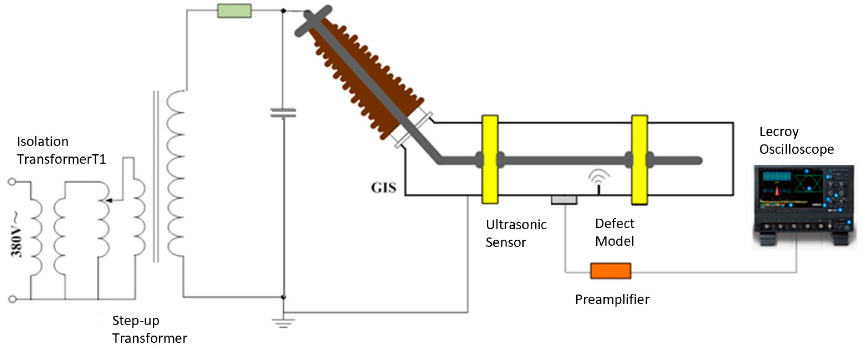
2.1. Experimental Setup

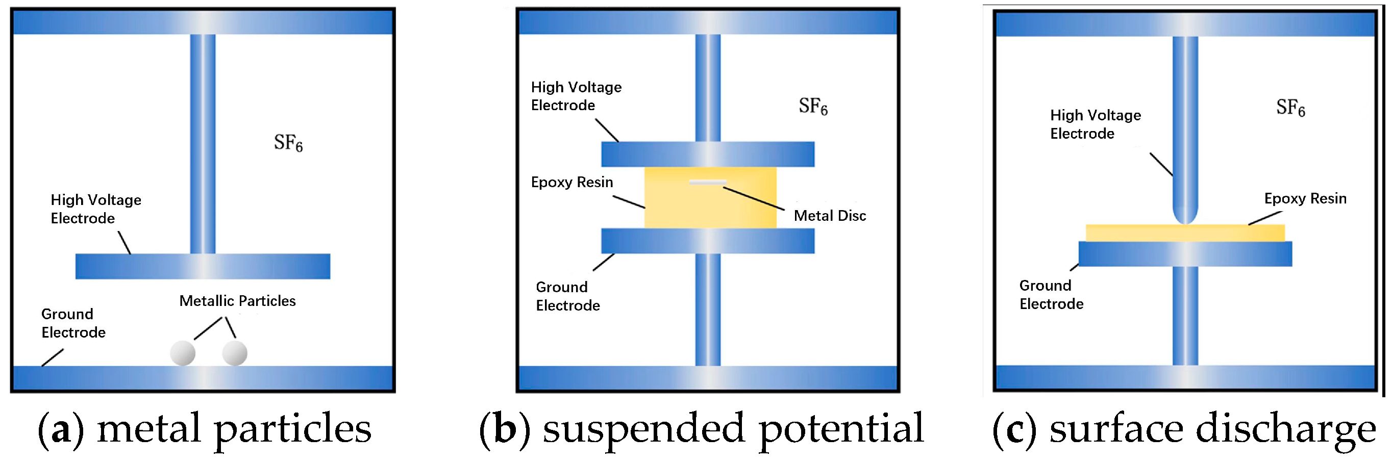
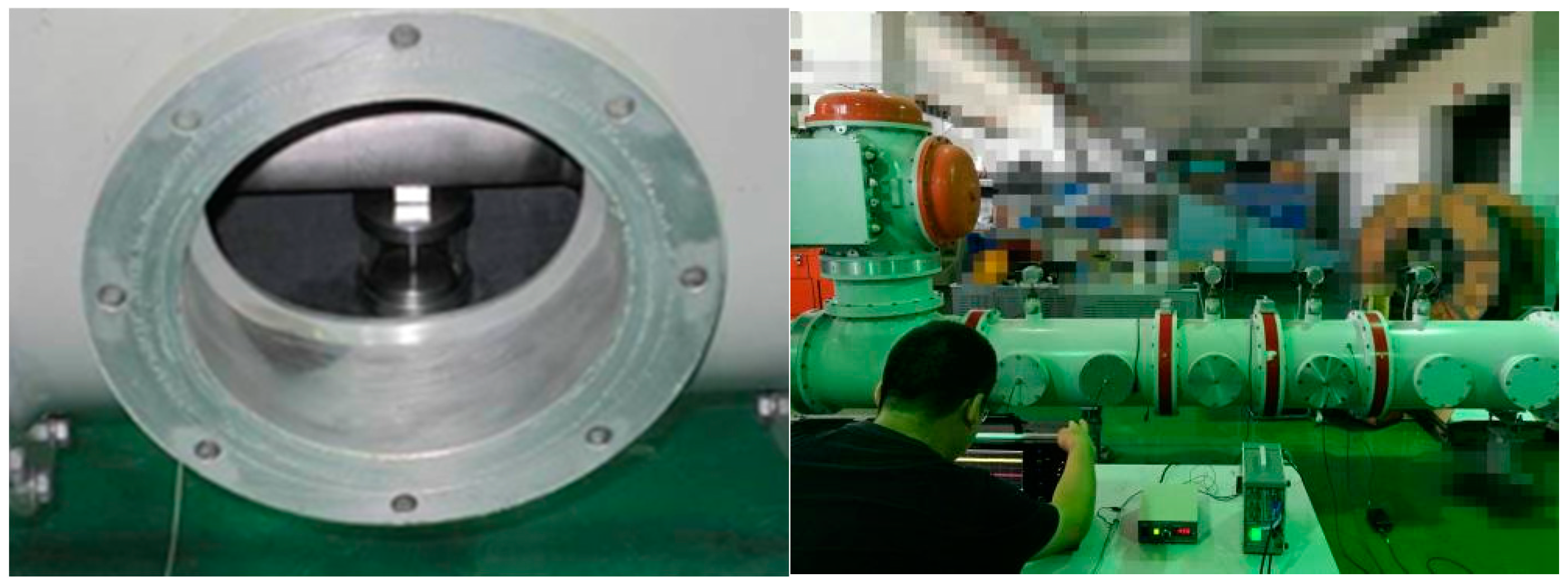
2.1.1. GIS Partial Discharge Test Platform and Defect Models

The GIS partial discharge test platform used mainly includes the ZF28A-145 type GIS test chamber manufactured by Sieyuan Electric, Shanghai, China, YDTW-25/100 type AC corona-free test transformer manufactured by Top Union, China, Wuhan, MAE-90 ultrasonic sensor manufactured by Jiangsu Baihang, China, Jiangsi, preamplifier (gain of 100/4.7), HDO6000A type LeCroy oscilloscope manufactured by RIGOL, China and other devices, as shown in Figure 1.

Three types of typical GIS insulation defects, namely free metal particles, suspended discharge, and surface discharge, were designed and constructed as shown in Figure 2. For the free metal particle defect, two small metal balls were placed between the high-voltage disc electrode and the grounded disc electrode to simulate the metal particles generated inside the GIS chamber. For the suspended discharge defect, a small metal round plate was sealed with epoxy resin between the high-voltage cylindrical electrode and the grounded disc electrode to simulate a detached or loose metal component inside the chamber. For the surface discharge defect, an epoxy resin board was placed between the high-voltage cylindrical electrode and the grounded disc electrode and connected to the high-voltage end to simulate the process of surface discharge within the GIS insulation.

2.1.2. Experimental Method

Before the experiment, the ultrasonic sensor was fixed to the surface of the GIS metal shell with an elastic band, and a layer of coupling agent was applied to the surface of the ultrasonic sensor to fill the air gap between the GIS shell and the sensor surface, ensuring the sensitivity of the ultrasonic sensor. The GIS test chamber was filled with SF6 gas at a pressure of 0.5 MPa as the insulating medium, and the oscilloscope sampling rate was set to 25 MS/s.

After checking the gas tightness of the GIS chamber, partial discharge tests for free metal particles, suspended discharge, and surface discharge were conducted separately. During the experiment, the voltage was gradually increased until the partial discharge signal appeared, and then the voltage was further increased until a stable and continuous partial discharge signal was obtained. The ultrasonic signals detected by the sensor were amplified by the preamplifier and then transmitted to the LeCroy oscilloscope to record and store the partial discharge data. The experimental site is shown in Figure 3.

2.2. GIS Partial Discharge Acoustic Identification Method

2.2.1. Wavelet Denoising

Wavelet transform is a common method for signal denoising and signal decomposition. By selecting wavelet basis functions for signal decomposition, threshold processing, and reconstruction, common wavelet basis functions include Daubechies wavelets, Symlet wavelets, Haar wavelets, and Meyer wavelets, etc.

Partial discharge signals typically exhibit transient and non-stationary characteristics. The sym4 wavelet can decompose the signal at different scales, capturing the high-frequency transient information while preserving the low-frequency background components. This multi-resolution analysis facilitates the effective separation of noise from the useful signal components. In this study, we selected the sym4 wavelet for denoising ultrasonic signals. Compared with the other wavelet bases mentioned above, sym4 possesses higher symmetry, which effectively reduces phase distortion and artifacts during wavelet coefficient thresholding and signal reconstruction, thereby better preserving the true nature of partial discharge signals.

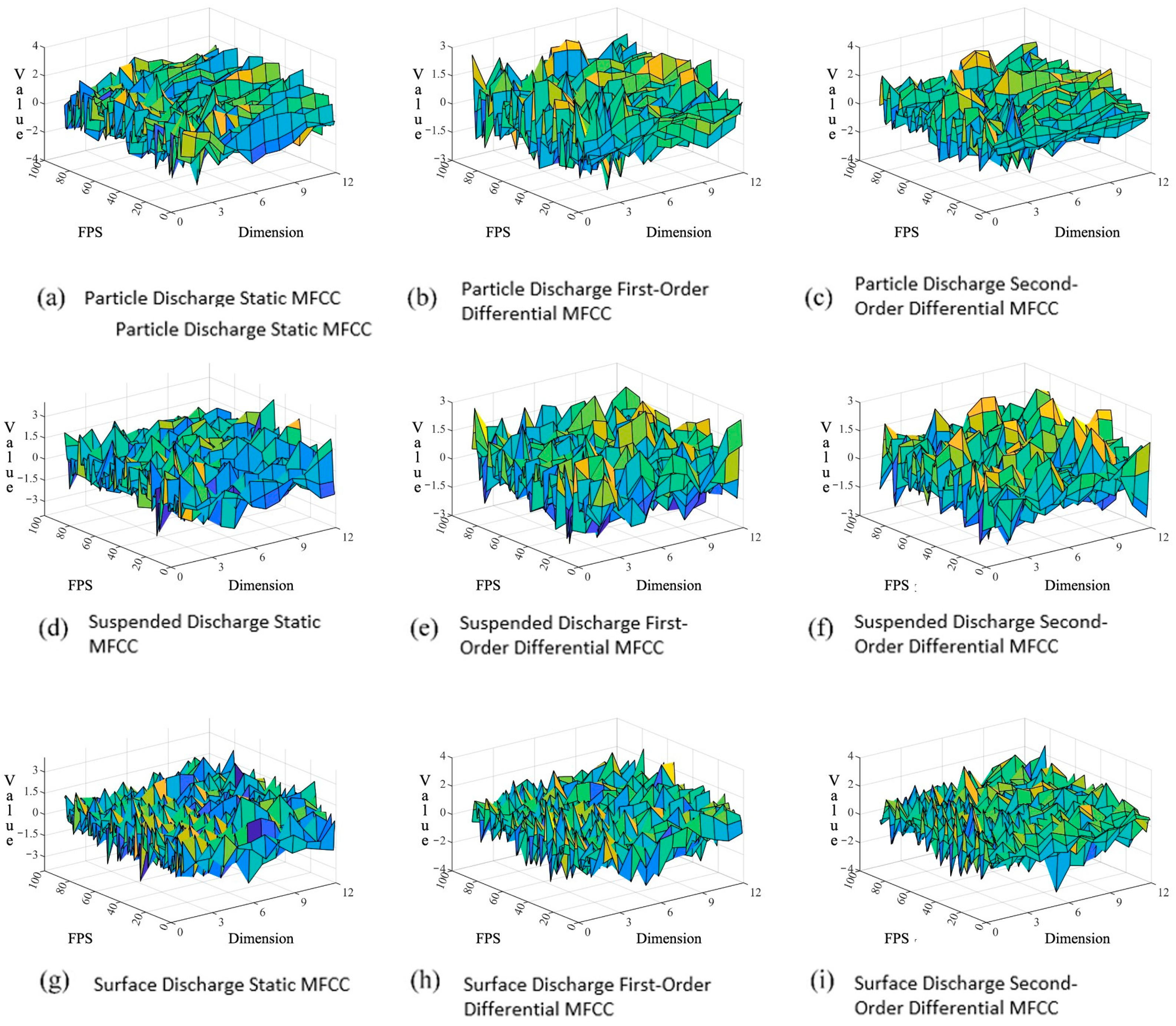
2.2.2. Improved MFCC Feature Parameter Extraction

MFCC transforms the input signal from the actual frequency domain to the mel frequency domain, and their relationship can be represented as:

$$f_{mel}=2952 \lg \left(1+{\displaystyle \frac{f}{700}}\right)$$

(1)

where $f_{mel}$ is the mel frequency and f is the actual frequency.

The MFCC parameters of the ultrasonic signal are selected as feature parameters, and the main steps of MFCC feature extraction are shown in Figure 4. The specific extraction steps are as follows:

(1) Pre-emphasis: Increase the energy of the high-frequency components of the acoustic signal to compensate for the high-frequency components suppressed by the sound production system. The calculation formula is:

$$y\left(t\right)=x\left(t\right)-\alpha x\left(t-1\right)$$

(2)

where x(t) and x(t − 1) are the original signals, y(t) is the pre-emphasized signal, and α is a constant, usually taken between 0.95 and 0.97, and in this paper, α is taken as 0.97.

(2) Framing and Windowing: In acoustic recognition, a frame length of 20–30 ms is usually taken, and MFCC parameters are extracted for each frame of signal. Considering the higher frequency of ultrasonic signals and the need to display the change characteristics of partial discharge pulses, a frame length of 20 ms, which is the length of a power frequency cycle, is taken in this paper. To ensure the continuity of the signal after framing, the next frame should overlap with part of the previous frame, and in this paper, an overlap rate of 50% is taken. Since the signal will undergo the Discrete Fourier Transform (DFT) after windowing, to ensure the continuity of the frames after the transform, the signal needs to be windowed after framing. In this paper, a Hamming window is added to the framed signal, and the relative calculation formula can be expressed as:

$$W\left(n,a\right)=\left\{\begin{array}{l}(1-a)-\mathrm{acos}\left({\displaystyle \frac{2\pi n}{N-1}}\right),0\le n\le N-1\\ 0, \mathrm{e}\mathrm{l}\mathrm{s}\mathrm{e}\end{array}\right.$$

(3)

where N is the length of the Hamming window, and a is a constant, generally taken as a = 0.46.

(3) FFT Transformation: The windowed signal undergoes FFT transformation to facilitate further analysis of signal characteristics in the frequency domain.

(4) Mel Filter Bank Filtering: The mel filter bank is composed of multiple triangular band-pass filters evenly distributed on the mel frequency. According to the sampling theorem, the maximum frequency of the filter should be half of the sampling frequency. The triangular band-pass filter can be expressed as:

$$H_m\left(f\right)=\left\{\begin{array}{l}\\ 0 , f(k)<f(m-1) \mathrm{o}\mathrm{r} f(k)>f(m+1)\\ {\displaystyle \frac{2\left[k-f\left(m-1\right)\right]}{\left[f\left(m+1\right)-f\left(m-1\right)\right]\left[f\left(m\right)-f\left(m-1\right)\right]}},f(m-1)\le f(k)\le f(m)\\ {\displaystyle \frac{2\left[f\left(m+1\right)-k\right]}{\left[f\left(m+1\right)-f\left(m-1\right)\right]\left[f\left(m+1\right)-f\left(m\right)\right]}},f(m)\le f(k)\le f(m+1)\end{array}\right.$$

(4)

where f(m) is the center frequency of the k-th filter in the linear spectrum.

(5) Logarithmic Calculation: The mel spectrum undergoes logarithmic calculation, and the calculation formula is:

$$S\left(m\right)=\ln \left[\sum _{k=0}^{N-1} |x(k){|}^2{H}_m(k)\right],0<m<M$$

(5)

where x(k) is the FFT of the framed signal, and N is the length of the FFT.

(6) Discrete Cosine Transform: After the discrete cosine transform, the obtained MFCC parameters can be expressed as:

$$c\left(i\right)=\sqrt{{\displaystyle \frac{2}{N}}}\sum _{j=1}^p m_j\cos \left[\left(j-0.5\right){\displaystyle \frac{\pi i}{M}}\right],1\le i,j\le M$$

(6)

where the calculated c(i) is the i-th dimension of the MFCC parameter with dimension M.

The above conventional MFCC parameter extraction method can truly reflect the static characteristics of the sound signal. However, for partial discharges caused by different insulation defects, the trend of ultrasonic signals over time varies greatly, and relying solely on static features is insufficient to fully reflect the change process of the partial discharge signal. Dynamic features reflect the temporal variations of a signal, providing richer information than static features, which helps improve the model’s recognition capabilities. Therefore, this paper introduces first-order and second-order differential improved MFCC parameters on the basis of conventional MFCC parameters to characterize the dynamic features of partial discharge, combining conventional MFCC with first-order and second-order differential MFCC as partial discharge feature parameters. The calculation formulas for first-order and second-order differential MFCC are:

$${\Delta }_n=\left\{\begin{array}{ll}{c}_{n+1}-c_n& ,n\le K\\ {\displaystyle \sum _{k=1}^K} k\left(c_{n+k}-c_{n-k}\right)& ,K+1\le n\le N-K\\ \sqrt{2{\displaystyle \sum _{k=1}^K} k^2}& ,K+1\le n\le N-K\\ c_n-c_{n-1}& , n\ge N-K+1\end{array}\right.$$

(7)

$$\Delta {\Delta }_n=\left\{\begin{array}{ll}{\Delta }_{n+1}-{\Delta }_n& ,n\le K\\ {\displaystyle \sum _{k=1}^K} k\left({\Delta }_{n+k}-{\Delta }_{n-k}\right)& ,K+1\le n\le N-K\\ \sqrt{2{\displaystyle \sum _{k=1}^K} k^2}& ,K+1\le n\le N-K\\ {\Delta }_n-{\Delta }_{n-1}& ,n\ge N-K+1\end{array}\right.$$

(8)

where n represents the n-th frame of MFCC parameters, Δ_n represents the first-order differential MFCC parameters of the n-th frame signal, and ${\Delta \Delta }_n$ represents the second-order differential MFCC parameters of the n-th frame signal.

Partial discharge signals typically exhibit high-frequency, transient characteristics and are often subject to environmental noise interference during actual measurements. By incorporating dynamic features into the basic MFCC parameters, it is possible to capture the dynamic variations of speech signals, increasing the model’s sensitivity to temporal changes and enhancing recognition performance.

2.2.3. Principal Component Analysis

The number of parameters obtained by the improved MFCC method is much larger than the conventional MFCC parameters, which can fully reflect the characteristics of GIS partial discharge ultrasonic signals. However, a large number of feature vectors input into the recognition model will increase the calculation time of the model. Therefore, to ensure that the different insulation defect partial parameters are presented, this paper uses principal component analysis (PCA) to reduce and optimize the dimension of the improved MFCC parameters, thereby improving the overall recognition efficiency. The implementation steps of principal component analysis are as follows:

(1)

For a matrix A of n m-dimensional feature parameters, it can be expressed as:

$$A=\left(\begin{array}{ccc}{a}_{11}& \cdots & a_{1m}\\ ⋮& \ddots & ⋮\\ a_{n1}& \cdots & a_{nm}\end{array}\right)$$

(9)

(2)

Calculate the covariance matrix. The n-dimensional correlation matrix of A can be expressed as:

$$R={\displaystyle \frac{1}{n-1}}{A}^{T}A$$

(10)

(3)

Calculate the eigenvalues ${\lambda }_1,{\lambda }_2,\dots ,{\lambda }_m$ of the covariance matrix R and their corresponding unit eigenvectors $p_1,p_2,\dots ,p_m$.

(4)

Sort the eigenvalues from largest to smallest, and arrange the eigenvectors in the same order. Calculate the contribution rate and cumulative contribution rate of each principal component based on the eigenvalues, which can be expressed as:

$${\eta }_i={\displaystyle \frac{{\lambda }_i}{\sum _i^m {\lambda }_i}}$$

(11)

$$\eta \left(k\right)=\sum _i^k {\eta }_i$$

(12)

where η(k) represents the cumulative contribution rate of the first k principal components, generally using the cumulative contribution rate as the parameter for dimensionality reduction.

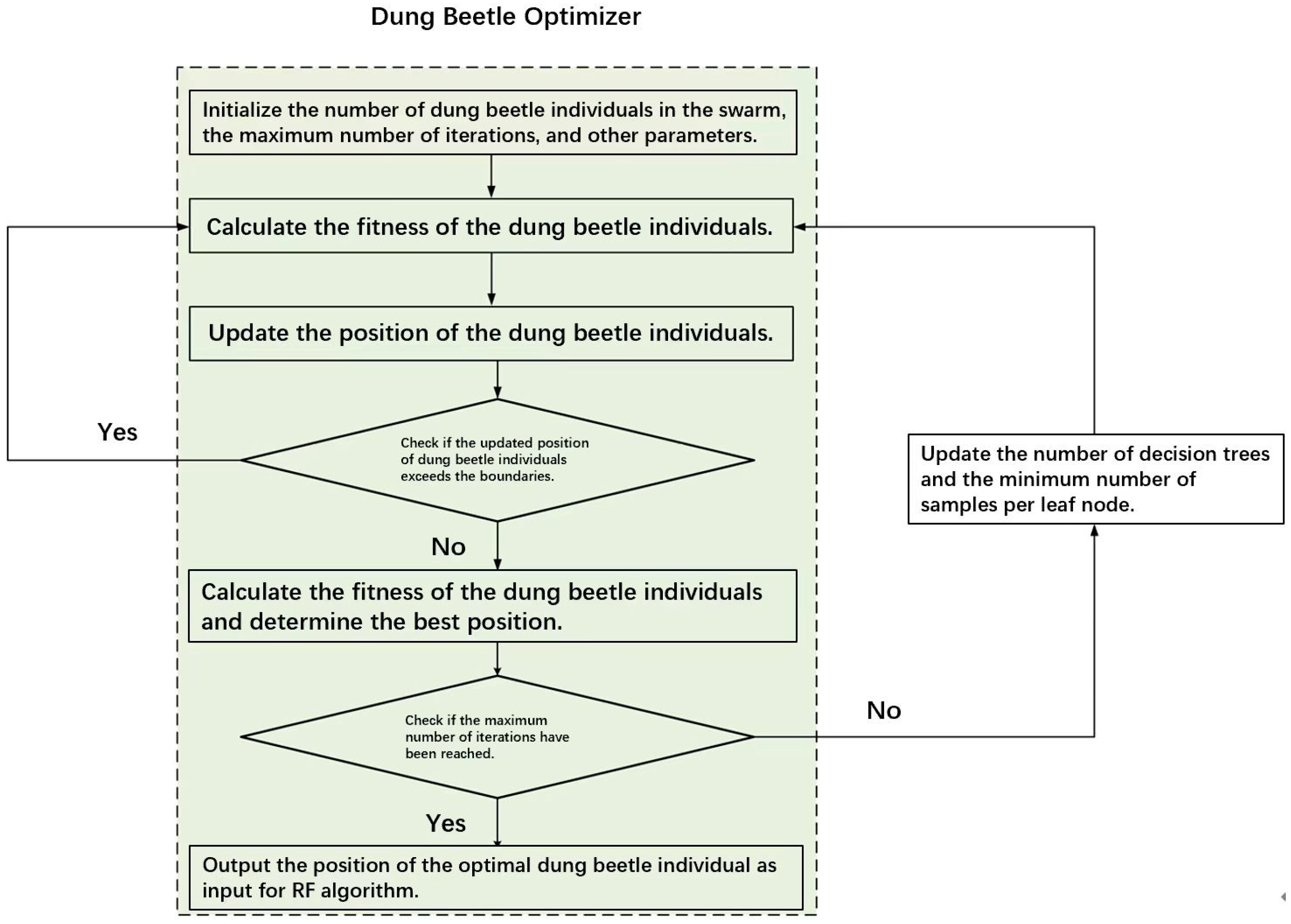
2.2.4. Dung Beetle Algorithm Optimized Random Forest Recognition Method

Dung Beetle Algorithm

The dung beetle algorithm (DBO) is a heuristic global optimization algorithm proposed by Shen Bo et al. [27], which exhibits a strong convergence speed. Its design typically involves simple iterative update rules and only a few control parameters, which allows the algorithm to find a near-optimal solution within a limited number of iterations. Defect detection systems often require real-time or near-real-time processing while maintaining high accuracy. Compared to more complex evolutionary algorithms, such as genetic algorithms and particle swarm optimization, the dung beetle optimization algorithm has a simpler structure and lower computational cost, thereby reducing the overall training time while still ensuring effective search performance.

The DBO simulates the life behavior of dung beetles in nature to search for the optimal solution of the target. Dung beetle individuals are divided into different roles based on different rolling, breeding, foraging, and stealing behaviors, and they update their positions with different strategies during the search process. Each dung beetle’s position represents a solution to the problem, and the final optimal position of the dung beetle is the optimal solution to the problem.

(1)

Rolling Behavior

The rolling behavior of dung beetles can be divided into obstacle-free and obstacle-laden modes based on whether obstacles are encountered. When there are no obstacles, dung beetles use the sun’s positioning to maintain the straight movement of the dung ball, and the position update of the dung beetle is affected by the intensity of sunlight. If obstacles are encountered, dung beetles cannot directly search for the optimal solution and turn to dancing behavior to obtain a new path. The above behavior can be abstracted into two different strategies for updating the positions of dung beetle individuals, and the position update strategy for the obstacle-free mode can be expressed as:

$$\left\{\begin{array}{l}{x}_i(t+1)=x_i\left(t\right)+\alpha k{x}_i(t-1)+b\Delta x\\ \Delta x=\left|x_i\left(t\right)-X^w\right|\end{array}\right.$$

(13)

where $x_i\left(t\right)$ is the position of the i-th dung beetle individual at the t-th iteration; the natural coefficient denoted as $\alpha$ controls the randomness in the beetle’s search process, determining the extent of random movement within the search space. Constraining $\alpha$ within the range of [−1, 1] ensures an appropriate magnitude of random perturbations, preventing excessive randomness that could lead to an uncontrolled search process, while also avoiding insufficient randomness that might cause the algorithm to become trapped in local optima; the deflection coefficient denoted as $k$ adjusts the beetle’s direction during the search process, representing the degree of deviation from the current search direction. Setting $k$ within the range of (0, 0.2) helps balance global exploration and local exploitation capabilities, enabling the algorithm to thoroughly explore the search space while also performing fine-tuned searches near potential solutions; $\Delta x$ represents the parameter characterizing the change in sunlight intensity; $X^w$ indicates the worst position in the global search; b is a constant with a range between (0, 1). In the obstacle-laden mode, the dancing behavior is represented by a tangent function, and the position update strategy can be expressed as:

$$x_i\left(t+1\right)=x_i\left(t\right)+\tan \left(\theta \right)\left|x_i\left(t\right)-x_i\left(t-1\right)\right|$$

(14)

where θ is a deflection angle with a range of [0, π], and θ equals 0, π/2, and π when the dung beetle does not update its position.

(2)

Breeding Behavior

Breeding behavior is a boundary selection strategy that simulates the dung beetle’s choice of spawning sites, and choosing a safe and suitable location to spawn is crucial for the offspring of the dung beetle population. Once a spawning area is selected, dung beetle individuals will spawn in that area, with each dung beetle laying only one egg per iteration. The calculation formula for the spawning position in breeding behavior is:

$$\left\{\begin{array}{c}{L}_b^{*}=\max (X^{*}\times (1-R),L_b)\\ U_b^{*}=\min (X^{*}\times (1+R),U_b)\end{array}\right.$$

(15)

where $L_b^{*}$ and $U_b^{*}$ represent the lower and upper bounds of the spawning area, respectively; $L_b$ and $U_b$ represent the lower and upper bounds of the search space, respectively; R is the inertia weight, $R=1-t/T_{\max };T_{\max }$ is the maximum number of iterations; $X^{*}$ is the optimal position of the current population of dung beetle individuals. From Equation (15), it can be analyzed that the boundary of the spawning area changes during the solution process, and the change in the spawning area boundary affects the optimal spawning position. The influence of the change in the spawning area boundary on the optimal spawning position can be expressed as:

$$B_i\left(t+1\right)=X^{*}+b_1\times \left(B_i\left(t\right)-L_b^{*}\right)+b_2\times \left(B_i\left(t\right)-U_b^{*}\right)$$

(16)

where $B_i\left(t\right)$ is the position of the i-th dung ball with eggs at the t-th iteration; $b_1 \mathrm{a}\mathrm{n}\mathrm{d} b_2$ represent two random vectors of size $1\times D;D$ represents the dimension of the optimization problem.

(3)

Foraging Behavior

Foraging behavior simulates the path selection process of dung beetles searching for food after growing up. In the algorithm, the best foraging area guides dung beetle individuals to update their paths to find food in a specified area based on their own position and the position of the food, ultimately obtaining the optimal solution. The boundary of the best foraging area can be defined as:

$$\left\{\begin{array}{c}{L}_b^b=\max (X^b\times (1-R),L_b)\\ U_b^b=\min (X^b\times (1+R),U_b)\end{array}\right.$$

(17)

where $L_b^b \mathrm{a}\mathrm{n}\mathrm{d} U_b^b$ represent the lower and upper bounds of the best foraging area, respectively; $X^b$ is the global optimal position. The calculation formula for the dung beetle’s foraging position update is:

$$x_i\left(t+1\right)=x_i\left(t\right)+C_1\times \left(x_i\left(t\right)-L_b^b\right)+C_2\times \left(x_i\left(t\right)-U_b^b\right)$$

(18)

where $B_i\left(t\right)$ is the position of the i-th dung beetle at the t-th iteration; $C_{1 }$ and ${ C}_{2 }$ are random numbers and random vectors obeying a normal distribution, respectively, with $C_{1 }$ obeying a normal distribution and $C_2$ being between (0, 1).

(4)

Stealing Behavior

Due to the competitive relationship between dung beetles in the struggle for food, stealing behavior simulates the behavior of dung beetle individuals stealing dung balls from other individuals during the rolling process. The position update strategy for the thief dung beetle individual can be expressed as:

$$x_i\left(t+1\right)=X^b+S\times g\times \left(\left|x_i\left(t\right)-X^{*}\right|+\left|x_i\left(t\right)-X^b\right|\right)$$

(19)

where $x_i\left(t\right)$ is the position of the i-th thief dung beetle at the t-th iteration; g represents a random vector of size $1\times D$ obeying a normal distribution, and S is a constant.

Random Forest Algorithm

The random forest (RF) is a machine learning algorithm that constructs decision trees through random sampling and classifies data based on the voting results of multiple decision trees. It has the advantages of high computational efficiency and strong noise resistance. The main steps of the random forest algorithm are as follows:

(1)

Randomly sample the dataset D with replacement to form K training sample sets $D_k$;

(2)

Divide the nodes to construct decision tree T(k), randomly select p features to split leaf nodes, and construct decision tree T(k) based on the minimum Gini index. The calculation method of the Gini index is:

$$gini\left(p\right)=1-\sum _{i=1}^n p^{2}i$$

(20)

(3)

After K rounds of training, obtain a classification model with K decision trees s₁(x), s₂(x),…, s_k(x), and choose the maximum number of votes as the final recognition result, which can be expressed as:

$$S\left(x\right)=\arg \underset{y}{\max } \sum _{k=1}^K I\left(s_k\left(x\right)=y\right)$$

(21)

Traditional methods like random search or grid search often tend to become trapped in local optima, especially in high-dimensional hyperparameter spaces, such as the number of trees, maximum depth, and minimum samples for splits. The DBO, by simulating the “rolling” behavior of dung beetles in searching for and transporting dung balls, effectively balances global exploration and local exploitation, ensuring thorough exploration of the entire search space to find the global or near-global optimal hyperparameter combinations. This balancing capability enables the optimized random forest to make more rational decisions in feature selection and node splitting, thereby enhancing defect recognition capabilities.

In defect recognition tasks, data typically contains noise and imbalance issues, and defect samples may be relatively scarce. The DBO, through random perturbations and diversity maintenance mechanisms, can avoid premature convergence to local optima and exhibits strong robustness to noisy data. Additionally, during the search process, the algorithm can adaptively adjust the search direction and step size based on the performance of the current solution, allowing the random forest model to obtain optimal hyperparameter settings across different datasets and defect types, thereby improving the model’s generalization ability.

This paper uses the dung beetle optimization algorithm, which has strong global optimization capabilities and few input parameters, to optimize the random forest for the recognition of three typical GIS partial discharges. The process is shown in Figure 5.

3. Results

A total of 180 groups of GIS partial discharge ultrasonic data were collected in the experiment, with 60 groups for each of the three types of insulation defects: free metal particles, suspended discharge, and surface discharge. The length of each group of data is 250 ms. The waveforms of the ultrasonic data for the three types of insulation defects after wavelet denoising are shown in Figure 6.

Based on the frame length and overlap rate determined in Section 2.2.2, the conventional, first-order, and second-order MFCC feature parameters were extracted from the ultrasonic signals after wavelet denoising. A single dataset signal can obtain 95 frames of MFCC feature parameters. The static MFCC features have 12 dimensions, and the first-order and second-order differences maintain the same dimensionality as the static MFCC features. Therefore, the improved MFCC parameter dimensions obtained for a single dataset are 36. To reduce the adverse effects of the large numerical differences between MFCC feature parameters of different dimensions on partial discharge recognition, the conventional MFCC features were subjected to Z-score standardization processing. The calculation formula is:

$$z={\displaystyle \frac{x-\mu }{\sigma }}$$

(22)

In the formula, x represents the individual data value, μ represents the mean of the partial discharge signal dataset, and σ represents the standard deviation of the partial discharge signal dataset.

After standardization, the improved MFCC features of the three types of insulation defect partial discharge ultrasonic signals are shown in Figure 7, which displays the static, first-order, and second-order difference MFCC feature parameters for the suspended potential defect partial discharge.

After obtaining the MFCC feature parameters for different insulation defect partial discharges, principal component analysis (PCA) is used to reduce the dimensionality of the MFCC. In PCA, a cumulative contribution rate between 85% and 95% is typically considered a reasonable range. Setting a threshold of 90% strikes a balance between information retention and dimensionality reduction. This approach avoids redundancy from retaining too many principal components and prevents information loss from retaining too few. Consequently, it reduces data dimensionality while preserving the primary characteristics of the original data, enhancing computational efficiency and reducing model complexity. After dimensionality reduction, the improved MFCC feature parameters for a single dataset are 95 × 15, and for the entire dataset, the improved MFCC feature parameters are 17,100 × 15.

Randomly select 12,500 frames from the entire dataset to input into the DBO-RF algorithm for partial discharge type identification, calculate the recognition accuracy of different feature parameters, compare to obtain the optimal feature parameters, and then select the RF, SVM, and KNN algorithms to compare with the recognition results of the DBO-RF algorithm to verify the effectiveness of the DBO-RF algorithm. The model is trained using the training set data, and the recognition results are obtained using the test set partial discharge data, with a training set to test set ratio of 8:2. The recognition results for different feature parameters are shown in

Table 1. Comparison of identification accuracy of different feature parameters.

Feature Parameters	Recognition Accuracy
Static MFCC	91.2%
First-order Differential MFCC	84.5%
Second-order Differential MFCC	82.4%
Static + Dynamic MFCC	90.5%
Static + Dynamic MFCC + PCA	92.2%

.

Analysis of Table 1 indicates that the combination of static + dynamic MFCC + PCA feature parameters achieves the most ideal recognition accuracy, with accuracy rates 1.10%, 9.11%, 11.89%, and 1.88% higher than other feature parameters, respectively. It can be seen that the recognition result of static MFCC is slightly lower than that of static + dynamic MFCC + PCA, and the recognition effect of using only first-order difference or second-order difference MFCC is poor. Therefore, this paper selects the static + dynamic MFCC + PCA feature parameters as the feature parameters for partial discharge recognition.

Table 2. Comparison of identification accuracy of different classification algorithms.

Algorithm Type	Recognition Accuracy
RF	90.7%
SVM	90.8%
KNN	89.6%
DBO-RF	92.2%

shows the recognition results of GIS partial discharge using different classification algorithms. The recognition accuracies of RF, SVM, and KNN algorithms are 90.7%, 90.8%, and 89.6%, respectively, while the DBO-RF algorithm has the best recognition effect on GIS partial discharge, with an accuracy rate reaching 92.2%. The recognition accuracy is improved by optimizing the parameters of the RF algorithm using the dung beetle algorithm. The DBO possesses adaptive adjustment capabilities, allowing it to dynamically modify its search strategy based on the current search state. This enables the random forest model to obtain optimal parameter settings when handling different types of partial discharge signals, thereby enhancing the model’s adaptability and robustness to diverse data. Through optimization, the structure of the decision trees within the random forest becomes more rational, reducing the risk of overfitting and improving the model’s stability and predictive performance on new data. By effectively optimizing the parameters of the random forest, the DBO enhances the model’s global search ability and balances exploration with exploitation, leading to higher accuracy in GIS partial discharge identification.

4. Discussion

This paper proposes an improved MFCC and DBO-RF algorithm-based acoustic recognition method for partial discharge detection using ultrasonic testing methods. It extracts the static, first-order difference, and second-order difference MFCC feature parameters of the GIS insulation defect partial discharge ultrasonic signals and applies principal component analysis (PCA) to dimensionally reduce and optimize the standardized feature parameters. Leveraging the strong global optimization capability and few input parameters of the DBO optimization algorithm, it identifies three typical GIS insulation defects: free metal particles, suspended discharge, and surface discharge. The results show that:

(1) The recognition accuracy of the static + dynamic MFCC + PCA feature parameters is the highest, demonstrating significant recognition effects on GIS insulation defect partial discharges.

(2) By comparing the recognition accuracies of DBO-RF with RF, SVM, and KNN algorithms, the optimization capability of DBO on the recognition accuracy of the RF algorithm for GIS insulation defect partial discharges is confirmed, with the optimized algorithm achieving a recognition accuracy of 92.2%.

References

1. Qiu, Y. GIS Devices and Insulation Technology; Xi’an Jiaotong University: Xi’an, China, 2007. [Google Scholar]
2. Gao, S.; Wang, C.; Li, F. Online Monitoring and Fault Diagnosis of Power Equipment; Tsinghua University: Beijing, China, 2018. [Google Scholar]
3. Zhang, S. Intelligent Diagnosis Method for Discharge Fault Mode of High Voltage SF6 Gas Insulated Switchgear. High Volt. Eng. 2020, 46, 432–440. [Google Scholar]
4. CIGRE Working Group 33/32-12. Insulation Co-ordination of GIS: Return of Experience, on Site Tests and Diagnostic techniques. Electra 1998, 176, 67–95. [Google Scholar]
5. Schichler, U.; Koltunowicz, W.; Endo, F.; Feser, K.; Giboulet, A.; Girodet, A.; Hama, H.; Hampton, B.; Kranz, H.G.; Lopez-Roldan, J.; et al. Risk assessment on defects in GIS based on PD diagnostics. IEEE Trans. Dielectr. Electr. Insul. 2013, 20, 2165–2172. [Google Scholar] [CrossRef]
6. Li, J.; Zhao, X.; Yang, J. Partial discharge measurement and analysis of typical defects in GIS. High Volt. Eng. 2009, 35, 2440–2445. [Google Scholar]
7. Chen, Y.; Chang, D.; Yang, D.; Zhang, G. PD creeping discharge development process induced by metallic particles in GIS. Electr. Power Eng. Technol. 2021, 40, 153–158. [Google Scholar]
8. Luo, L.; Yao, W.; Wang, J. Study on SF6 decomposition gas for partial discharge diagnosis in GIS. Power Syst. Technol. 2010, 34, 225–230. [Google Scholar]
9. Li, D.; Liang, J.; Bu, K. Ultrasonic detection of Partial Discharge of Typical Defects in GIS. High Volt. Appar. 2009, 45, 72–75. [Google Scholar]
10. Chen, F.; Tang, H.Z.; Li, H.G. Application of on-line ultrasonic and UHF partial discharge detection in 1000kV GIS. Appl. Mech. Mater. 2014, 644, 3480–3484. [Google Scholar] [CrossRef]
11. Wang, T.; Ding, H.; Zhang, Z. A partial discharge pattern recognition method based on deep learning and multi-model fusion. Electr. Power Eng. Technol. 2023, 42, 188–195. [Google Scholar]
12. Han, S.; Lv, Z.; Sui, H. Partial discharge pattern recognition in GIS based on EFPI sensor. Electr. Power Eng. Technol. 2022, 41, 149–155. [Google Scholar]
13. Gao, W.; Ding, D.; Liu, W. Research on the typical partial discharge using the UHF detection method for GIS. IEEE Trans. Power Deliv. 2011, 26, 2621–2629. [Google Scholar]
14. Xu, Y.; Liu, W.; Chen, W. Motion Characteristics and Partial Discharge Characteristics of Sub-millimeter Metal Particles on the Surface of AC GIS Spacer. Proc. CSEE 2019, 39, 4315–4324+4334. [Google Scholar]
15. Luo, S.; Tian, Y.; Li, B.; Hu, Y.; Li, Q. Pattern recognition of ultra-high frequency partial discharge by using scale parameters-energy entropy characteristic pairs. Electr. Power Eng. Technol. 2019, 38, 152–158. [Google Scholar]
16. Luo, Y.; Qi, B.; Chen, W. Study on Optical Detection Method of the Surface Weak Discharge of GIS Basin Insulator. Power Syst. Technol. 2024, 48, 4377–4386. Available online: http://kns.cnki.net/kcms/detail/11.2410.tm.20240425.1737.005.html (accessed on 12 September 2024).
17. Han, X.; Liu, Z.; Li, J. Study on PD Detection Method in GIS Based on the Optical and UHF Integrated Sensor. Proc. CSEE 2018, 38, 6760–6769. [Google Scholar]
18. Hu, Z.; Li, Z.; Chen, H. Transformer state detection and assessment method based on voiceprint compression and cost-sensitive techniques. Electr. Power Eng. Technol. 2024, 43, 209–216. [Google Scholar]
19. Lawson, A.; Vabishchevich, P.; Huggins, M.; Ardis, P.; Battles, B.; Stauffer, A. Survey and evaluation of acoustic features for speaker recognition. In Proceedings of the 2011 IEEE International Conference on Acoustics, Speech and Signal Processing (ICASSP), Prague, Czech Republic, 22–27 May 2011; pp. 5444–5447. [Google Scholar]
20. Wang, R.; Li, R.; Chen, D. Sound recognition in low signal-to-noise ratio traffic environment based on improved wavelet packet denoising and Mel-cephalogram coefficients. Sci. Technol. Eng. 2019, 19, 290–295. [Google Scholar]
21. Logan, B. Mel frequency cepstral coefficients for music modeling. Ismir 2000, 270, 11. [Google Scholar]
22. Lv, X.; Wang, H. Abnormal sound recognition algorithm based on MFCC and short-time energy mixing. J. Comput. Appl. 2010, 30, 796–798. [Google Scholar]
23. Zhao, H.; Cong, P.; Li, C.; Qu, D.; Wei, H. GIS mechanical fault detection method based on vector space state optimization. High Volt. Appar. 2024, 60, 65–72. [Google Scholar]
24. Lu, Y.; Liao, C.; Li, Q.; Wang, T.; Shao, J.; Zhang, Y. Transformer fault diagnosis method based on voiceprint feature and ensemble learning. Electr. Power Eng. Technol. 2023, 42, 46–55. [Google Scholar]
25. Zhuang, X.; Li, Q.; Liu, Z.; Zhang, L.; Ji, T.; Zhang, C. GIS abnormal working condition voiceprint recognition algorithm based on improved MFCC-OCSVM and Bayesian optimized BiGRU. Power Syst. Technol. South. Power Syst. Technol. 2025, 19, 30–40. Available online: http://kns.cnki.net/kcms/detail/44.1643.tk.20240625.0913.018.html (accessed on 12 September 2024).
26. Xu, M.; Li, Z.; Sun, H. GIS mechanical fault diagnosis method based on improved Mel-frequency cepstral coefficients. High Volt. Appar. 2020, 56, 122–128. [Google Scholar]
27. Xue, J.; Shen, B. Dung beetle optimizer: A new meta-heuristic algorithm for global optimization. J. Supercomput. 2023, 79, 7305–7336. [Google Scholar]
Figure 1. GIS partial discharge test platform.
Energies 18 01619 g001
Figure 2. GIS partial discharge insulation defect model.
Energies 18 01619 g002
Figure 3. GIS partial discharge experimental site.
Energies 18 01619 g003
Figure 4. Flow chart of extracting MFCC features.
Energies 18 01619 g004
Figure 5. Flow chart of dung beetle optimization algorithm optimization random forest algorithm.
Energies 18 01619 g005
Figure 6. De-noising GIS partial discharge ultrasonic time domain waveform.
Energies 18 01619 g006
Figure 7. MFCC features of ultrasonic partial discharge signal of suspended potential defect.
Energies 18 01619 g007