Article

Multi-Time-Scale Layered Energy Management Strategy for Integrated Production, Storage, and Supply Hydrogen Refueling Stations Based on Flexible Hydrogen Load Characteristics of Ports

1
Three Gorges Electric Energy Co., Ltd., Wuhan 430015, China
2
China Yangtze Power Co., Ltd., Beijing 100033, China
3
Institute of Electrical Engineering, Chinese Academy of Sciences, Beijing 100190, China
*
Author to whom correspondence should be addressed.
Energies 2025, 18(7), 1583; https://doi.org/10.3390/en18071583
Submission received: 24 January 2025 / Revised: 4 March 2025 / Accepted: 13 March 2025 / Published: 22 March 2025
(This article belongs to the Special Issue Energy Storage Technologies and Applications for Smart Grids)

Abstract

:
Aiming at resolving the problem of stable and efficient operation of integrated green hydrogen production, storage, and supply hydrogen refueling stations at different time scales, this paper proposes a multi-time-scale hierarchical energy management strategy for integrated green hydrogen production, storage, and supply hydrogen refueling station (HFS). The proposed energy management strategy is divided into two layers. The upper layer uses the hourly time scale to optimize the operating power of HFS equipment with the goal of minimizing the typical daily operating cost, and proposes a parameter adaptive particle swarm optimization (PSA-PSO) solution algorithm that introduces Gaussian disturbance and adaptively adjusts the learning factor, inertia weight, and disturbance step size of the algorithm. Compared with traditional optimization algorithms, it can effectively improve the ability to search for the optimal solution. The lower layer uses the minute-level time scale to suppress the randomness of renewable energy power generation and hydrogen load consumption in the operation of HFS. A solution algorithm based on stochastic model predictive control (SMPC) is proposed. The Latin hypercube sampling (LHS) and simultaneous backward reduction methods are used to generate and reduce scenarios to obtain a set of high-probability random variable scenarios and bring them into the MPC to suppress the disturbance of random variables on the system operation. Finally, real operation data of a HFS in southern China are used for example analysis. The results show that the proposed energy management strategy has a good control effect in different typical scenarios.

1. Introduction

Fossil energy is currently responsible for most of the worldwide energy supply. However, the widespread usage of fossil energy can lead to serious environmental pollution problems [1]. Therefore, all countries around the world need to continuously explore new measures to save energy and reduce emissions [2]. As a clean energy, hydrogen energy has great potential for future development. It is an effective solution for energy saving and emission reduction at ports. The formation of HFSs can meet ports’ demands for the production of hydrogen-powered equipment [3]. However, traditional industrial hydrogen production still causes high carbon emissions, and the production of green hydrogen through renewable energy sources and the construction of an integrated green hydrogen production–storage–supply refueling process can greatly reduce carbon emissions [4]. However, the strong randomness of renewable energy generation in ports and the uncertainty of hydrogen load changing with the production characteristics of ports pose a greater challenge to the economic and stable operation of HFS systems. In addition, different electrical and hydrogen equipment at HFSs are coupled with each other, which makes it difficult to independently regulate different forms of energy. The energy management strategy can effectively promote the energy balance of the system, extend the service life of the equipment, reduce the system operating costs, and stabilize hydrogen supply, thus promoting the stable and efficient operation of a green hydrogen production, storage, and supply system [5].
The current studies on energy management of HFSs mainly consider two aspects: economy and decarbonization. Reference [6] established stochastic variable models including photovoltaic power generation and hydrogen consumption by hydrogen fuel vehicles and proposed an energy management strategy for the stochastic model to improve the profit of HFSs. Reference [7] proposed a two-layer optimization model in which the upper layer maximized the revenue of the HFS and the lower layer minimized the cost of the HFS, and the proposed energy management strategy had a better control effect compared with the single-layer model. Reference [8] proposed a seasonal hydrogen storage system energy management strategy to meet the demand for industrial hydrogen equipment for a hydrogen refueling system integrating photovoltaic power, an energy storage system, and hydrogen storage system. The energy management strategy for industrial hydrogen equipment uses the uncertainty of the electricity price to guide hydrogen storage planning to significantly improve economic performance. Aimed at achieving an off-grid renewable energy hydrogen refueling scenario, reference [9] obtained optimal operation schemes for different equipment and analyzed the impact of equipment configuration parameters on the energy scheduling results based on total life cycle cost minimization. For the operation mode of HFSs participating in the auxiliary service of the electricity market, reference [10] proposed an energy optimization strategy to maximize the profit while satisfying the hydrogen demand of downstream operators. Reference [11] took an HFS, including hydrogen production, storage, and fuel cell, as the research object, and considered the sum of the investment cost, operation and maintenance costs, and replacement cost as the optimization goal. An improved intelligent optimization algorithm was proposed for solving this problem, which caused the convergence process to be significantly improved. Reference [12] used the HFS of a tram as the research object and took the minimization of the sum of the electricity cost of the whole station as the optimization objective, which significantly reduced the operation cost of the whole station. Reference [13] proposed a two-layer energy optimization management strategy and used the elite genetic algorithm, which could reduce the operation cost, improve the self-sustaining rate, and reduce carbon emission. Reference [14] proposed a tri-level energy schedule method considering the uncertainties of prices, demands, solar irradiation, and wind speed. The profitability of the operation could be verified through a renewable-rich 69-bus system. However, the above-mentioned energy management strategies only research day-ahead operation economy. Reference [15] proposed a two-stage (day-ahead and intra-day) optimal scheduling strategy taking the operating economy and risk robustness into account, and the proposed algorithm effectively improved the economic benefits. However, the stable operation of the system on a minute scale was still ignored.
Essentially, HFS energy management is a problem with high-dimensional, nonlinear, and multi-constraint characteristics. The solving algorithms for energy management in HFSs mainly include programming methods, the MPC method, heuristic optimization algorithms, etc. Programming methods mainly include mixed integer programming, stochastic programming, robust programming, etc. However, programming algorithms consume a large amount of computing resources and are not capable of achieving real-time decision-making. Some programming algorithms excessively rely on accurate prediction of renewable energy generation and load, which is difficult to achieve in practical scenarios [16]. The algorithm based on MPC has a poor ability to handle the randomness of sources and loads [17]. Compared with programming solving algorithms, heuristic optimization algorithms can effectively solve problems with large data volumes and complex scenarios, but there is still a possibility of falling into the local optimal trap, thus not being able to obtain the true global optimal solution. Therefore, it is necessary to improve the solving performance of traditional heuristic optimization algorithms [18].
In summary, most of the existing energy management strategies mainly consider the day-ahead time scale, and the optimization objection mainly consider the economic aspect including investment cost, maintenance cost, and renewable energy consumption. However, the randomness of the source and loads on smaller time scales (e.g., minute-level) will lead to relatively intense fluctuations of equipment, which can bring more challenges to the stable operation of the hydrogen production and supplementation process. Few studies are currently available in this area.
Based on the above issues, a multi-time-scale hierarchical energy management strategy for integrated production, storage, and supply HFS is proposed. The main contributions of this paper are summarized as follows:
  • The upper layer considers minimizing the HFS daily operating costs, including operation and maintenance costs, purchased electricity cost, and purchased hydrogen cost. A PSA-PSO algorithm is proposed to solve the upper-layer energy management, thus improving the solving efficiency;
  • The objective function of the lower layer is to minimize the intra-day and day-ahead scheduling errors and the power fluctuations of the electrolyzer (Elz) and grid. The SMPC algorithm for solving the optimization problem is proposed to reduce the interference of stochastic variables and achieve better optimization results;
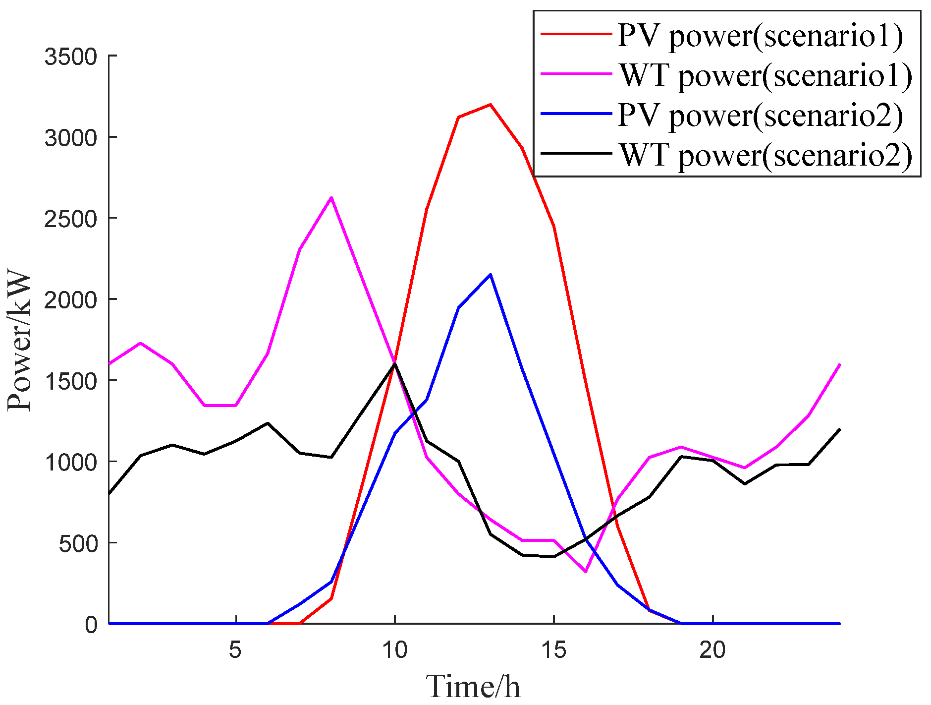
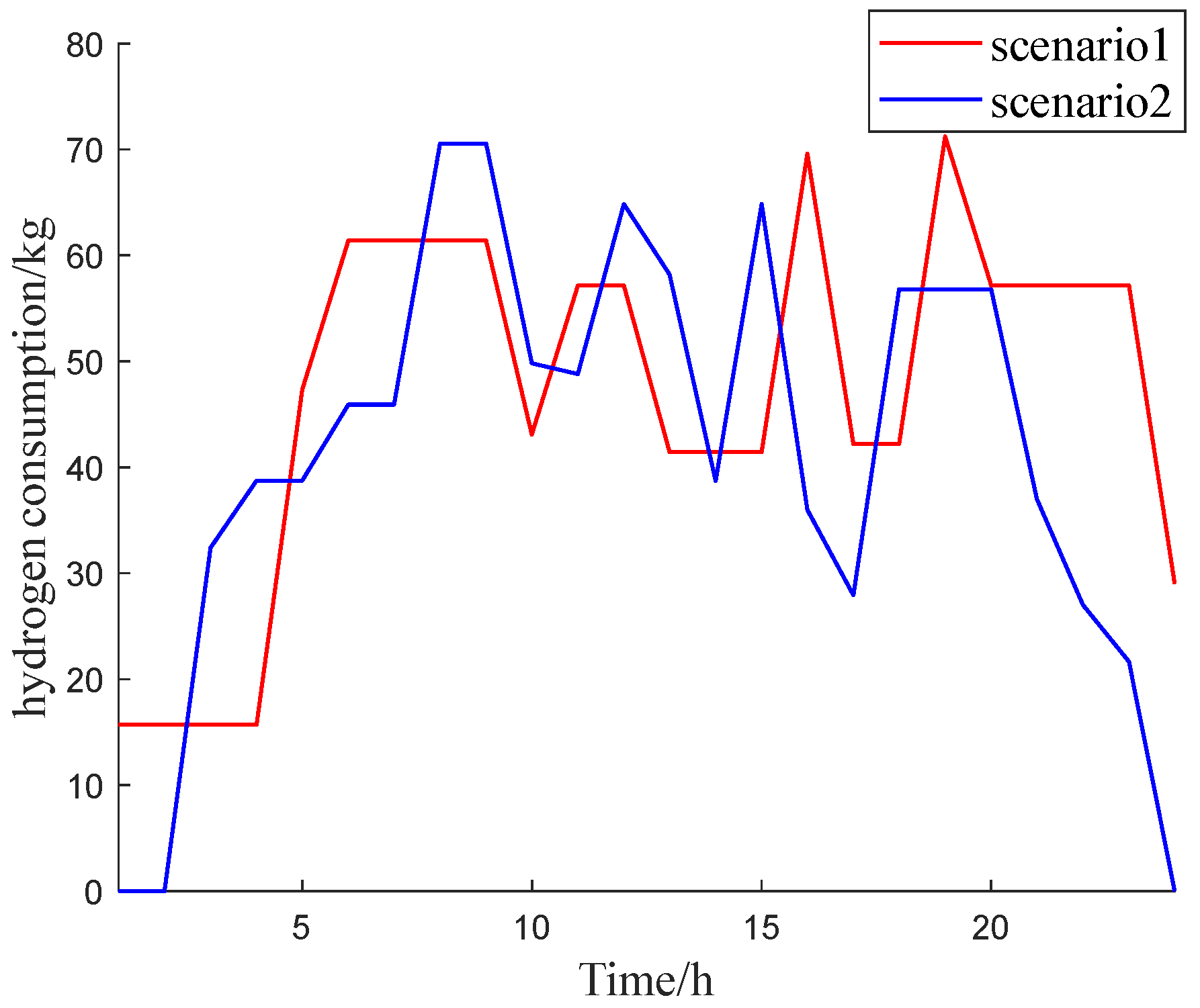
  • An example analysis is conducted using measured data from southeastern China to verify the proposed energy management. The results show that the proposed energy management strategy has good control effects in different typical scenarios.

2. Guidelines for Manuscript Preparation

The structure of the green hydrogen production, storage, and supply integrated HFS is shown in Figure 1, and the system adopts a DC bus structure, which has a relatively simple control process [19]. Wind turbine (WT) and photovoltaic (PV) equipment are used as the main power supply equipment in the HFS, lithium (LiB) is used as the main equipment to cope with the imbalance between the supply and demand of electricity, and the grid is used as a supplement. The HFS achieves the balance of local hydrogen supply and demand through the power-to-hydrogen (P2H) link including the Elz, compressor (CP), hydrogen storage tank (HST), and external hydrogen purchase. Due to the energy storage of the hydrogen storage tank, the P2H link affects the real-time power balance of the system at the same time, and the system power can also indirectly coordinate the hydrogen balance, since the hydrogen fuel mainly comes from the P2H process.

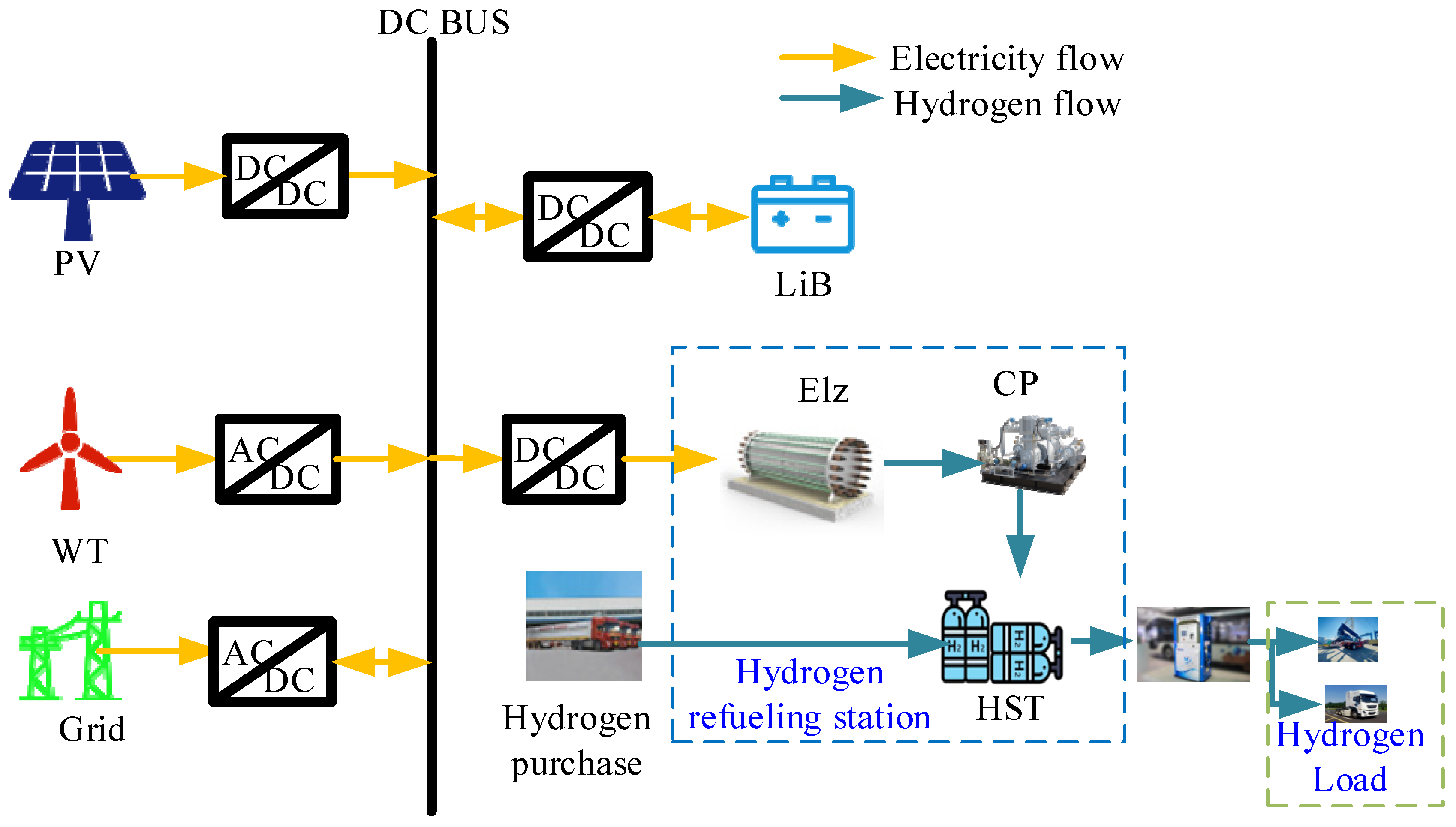
3. Multi-Time-Scale Energy Management Strategies

The overall framework of the multi-time scale-hierarchical energy management strategy for HFS proposed in this paper is shown in Figure 2. The upper layer takes the hour-level time scale as the research object, with the optimization objective of minimizing the sum of daily operation and maintenance costs, electricity purchase cost, and hydrogen purchase cost of a port HFS. The lower layer takes the minute-level time scale as the research object, with the regulation goal of reducing the interference of renewable energy and hydrogen load in the system.

3.1. Upper-Layer Energy Management Strategy

The upper layer generates scheduling instructions every hour on an hourly scale. This strategy mainly considers the economic aspect, which can be divided into three parts. The first part is the operation and maintenance cost of the HFS equipment, which includes the operation and maintenance costs of the Elz and LiB. The second part is the cost of purchasing electricity from the external grid, which can charge LiB or participate in hydrogen production when renewable energy power generation is in the trough, and consume excess electricity when renewable energy power generation is at the peak. The third part is the cost of purchasing hydrogen from the external hydrogen source. When the daily hydrogen consumption is at its peak, hydrogen production solely through local electrical equipment may not meet the demand. At this time, hydrogen needs to be purchased from external hydrogen sources. The goal of upper-layer energy management is to minimize the sum of the above three items:
C upper = min ( C op + C grid + C off ) = min t = 1 24 ( C bat P bat ( t ) + C ele P ele ( t ) + C fee P grid ( t ) + C H m off ( t ) )
where Cupper represents the upper-layer objective function, Cop represents the operation and maintenance cost of the equipment, Cgrid represents the external electricity purchase cost, Coff represents the cost of purchasing hydrogen from an external source, Cfee represents the electricity purchase price, Pgrid represents the power of the grid, and Cbatt and Cele respectively represent the operation and maintenance coefficients of LiB and Elz per unit power. CH is the per kilogram hydrogen price and moff represents the mass of hydrogen transported from external hydrogen sources.
The constraints that upper-layer energy management needs to meet include:
(1)
LiB mainly includes charging and discharging power constraints and state of charge (SOC) constraints:
P batmin P bat ( t ) P batmax S O C ( t + 1 ) = ( 1 R ) S O C ( t ) + P bat ( t ) η bat Δ T / E bat S O C min S O C ( t ) S O C max
where Pbatmin, Pbatmax, R, ηbat, SOCmin, SOCmax, Ebat, and ΔT represent the minimum operating power of the LiB, the maximum operating power of the LiB, self-discharge rate of LiB, charge/discharge rate of LiB, the minimum SOC value of the LiB, maximum SOC value of the LiB, capacity of the LiB, and time interval of the scheduling cycle. If Pbat is positive, the LiB is charging. Otherwise, the LiB is discharging.
(2)
The constraints of the Elz mainly include operating power constraints and hydrogen production constraints. The Elz operating power range is from minimum operation to rated power operation, and the minimum power of the Elz is usually 10% of its rated power [20,21]:
P elemin P ele ( t ) P elemax m h 2 ( t ) = η ele P ele ( t ) H H V
where Pelemin, Pelemax, HHV, and ηele represent the minimum operating power of the Elz, the maximum operating power of the Elz, the high heat value of hydrogen, and the efficiency of the Elz.
(3)
The operation of the CP mainly considers its power consumption, and its value is directly related to the hydrogen production of the Elz [22]:
P com = C p T in η comp ( ( P o u t P in ) r 1 r 1 ) n h 2
where Cp is the calorific value of hydrogen, Tin is the temperature of hydrogen at the inlet (K), ηcomp denotes the compress efficiency, which is taken as 0.7 in this paper, Pin and Pout denote the inlet and outlet pressures of the CP, r denotes the isentropic exponent of the hydrogen, which is usually taken as 1.4, and nh2 denotes the flow rate of the hydrogen. The hydrogen flow rate of CP is directly from the Elz, which can be expressed as [23]:
n h 2 ( t ) = η F n c I el ( t ) Z F
where nc is the number of cells connected in series in the Elz, Iel is the Elz current, Z is the number of charges transferred during the electrolysis of water, F denotes the Faraday constant, and ηF is the current efficiency of the Elz, which means the ratio of the charge required for the production of hydrogen to the total charge consumed by the Elz:
η F = b 1 + b 2 e ( b 3 + b 4 × T ae + b 5 × T ae 2 I el / A )
(4)
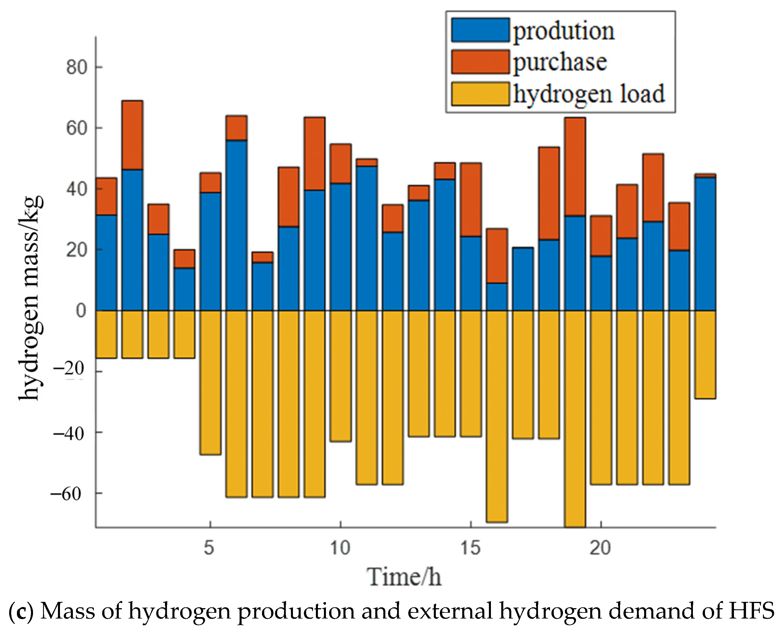
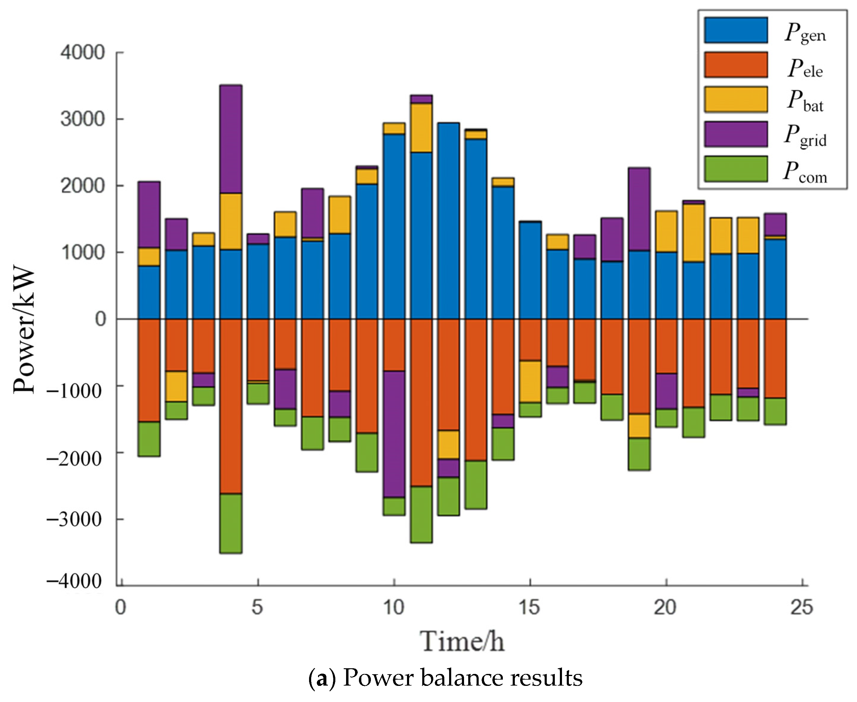
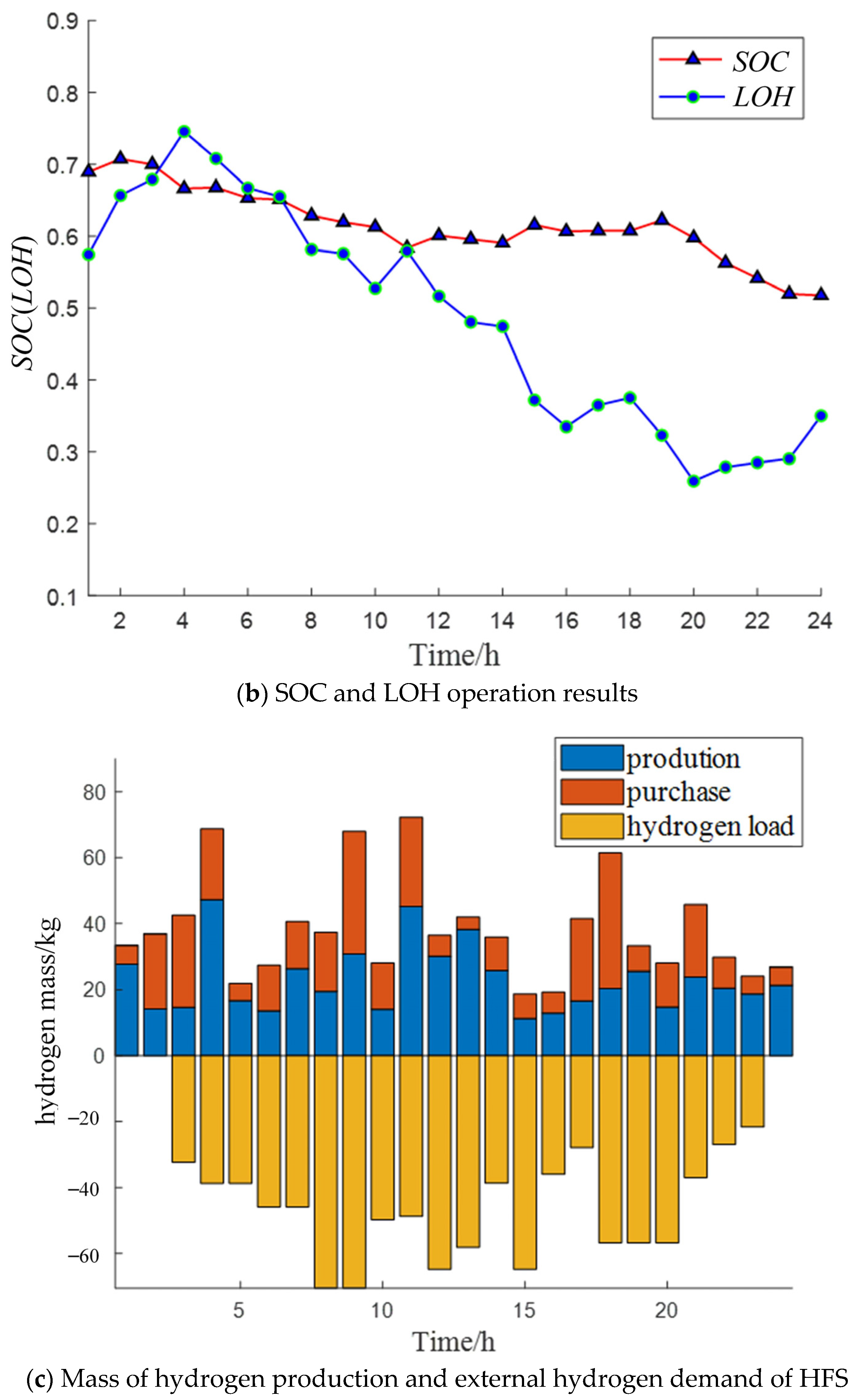
The level of hydrogen (LOH) is a key parameter to characterize the internal hydrogen storage amount of HST, which needs to meet the following constraints:
L O H ( t ) = m store ( t ) m max L O H ( t + 1 ) = L O H ( t ) + ( m h 2 ( t + 1 ) + m off ( t + 1 ) m load ( t + 1 ) ) Δ T / m max L O H min L O H ( t ) L O H max
where LOHmin, LOHmax, mstore, moff, mload, and mmax respectively represent the minimum LOH value, the maximum LOH value, the internal hydrogen mass of the HST, the mass of external hydrogen source supply, the hydrogen load demand, and maximum allowable hydrogen mass allowed to be stored in the HST.
(5)
At the end of each day, SOC and LOH are required to meet the operational requirements of the following day:
a min SOC 0 S O C ( 24 ) a max SOC 0 a min L O H 0 L O H ( 24 ) a max L O H 0
where SOC0 and LOH0 denote the initial values of SOC and LOH, respectively. amin and amax denote the SOC constraint coefficients. Taking the coupling relationship between different constraints into account, amin and amax are taken as 0.7 and 1.2, respectively.
(6)
The power of the grid needs to meet certain constraint:
P gridmin P grid ( t ) P gridmax
where Pgridmin and Pgridmax respectively represent the minimum and maximum power of the grid.
(7)
The electricity of the system needs to be balanced:
P pv ( t ) + P wt ( t ) = P ele ( t ) + P com ( t ) + P grid ( t ) + P bat ( t )
where Ppv and Pwt represent power of the PV and WT.
The PSO algorithm is widely used due to the advantages of easy operation, high degree of implementation, and high accuracy. This algorithm initializes a set of random particles and finds the optimal solution through continuous iteration. During the iteration process of the algorithm, the speed and position of particles are continuously modified through individual and global extreme values. The current optimal solution found by particles is called the individual extreme value, while the current optimal solution found by the population is called the global extreme value. The equation for updating the velocity and position of particles is [24]:
V ij ( t + 1 ) = ω × V ij ( t ) + C 1 × r 1 × [ P ij ( t ) X ij ( t ) ] + C 2 × r 2 × [ p gj ( t ) X ij ( t ) ] X ij ( t + 1 ) = X ij ( t ) + V ij ( t + 1 )
where j represents the search space dimension, i represents the number of particles, V represents the particle velocity, X represents the particle position, ω represents inertia weight, C1 and C2 represent learning factors, and r1 and r2 are all random numbers within [0, 1].
However, the traditional PSO algorithm has problems such as slow convergence speed and easily falling into local extremes. To address these issues, this paper proposes a PSA-PSO algorithm for solving upper-layer energy management. The main improvement measures include the following three aspects:
(1)
In the PSO algorithm, ω directly affects the global search ability [25]. A larger inertia weight has a stronger global search ability so the algorithm is more likely to obtain the optimal solution, while a smaller inertia weight will give particles a stronger local search ability and accelerate the convergence of the algorithm. Therefore, this paper adaptively adjusts the inertia weight. In the early stage, it can quickly obtain the optimal solution by achieving a larger ω. In the later stage of the iteration process, a lower ω is beneficial to algorithm convergence.
ω = ω max ( ω max ω min ) t 1 M a x i t
where ωmax and ωmin represent the upper and lower limits of the weight coefficient. In this paper, 0.9 and 0.4 are taken, respectively. t1 represents the current number of iterations, and Maxit represents the maximum number of iterations, which is set to 100.
(2)
The learning factors C1 and C2 are also important parameters for regulating algorithm performance. At the beginning of the algorithm iteration, so that the particles can search in the whole space, larger C1 and smaller C2 can be set. As the number of iterations increases, to make the particle search results more inclined toward the global optimal solution, larger C2 and smaller C1 are set. Additionally, to enhance the adaptive adjustment capability of parameters, the sine function and tangent function are applied in the formula for parameter adjustment, namely:
C 1 = C 1 max 1.5 sin ( t 1 / M a x i t ) C 2 = C 2 min + 1.5 tan ( t 1 / M a x i t )
where C1max and C2min are taken as 2 and 0.5, respectively.
(3)
This paper introduces Gaussian disturbance after each particle updates position to enhance particle diversity and jumps out of the local optimal solution. At the same time, an adaptive disturbance step size is set. As the number of iterations increases, the disturbance component gradually increases, thereby enhancing the ability to quickly search for the optimal solution. Namely:
X ij = X ij × ( 1 + μ × G a u s s ) μ = ( t 1 / M a x i t )
where μ represents disturbance step size and Gauss represents the Gaussian disturbance term.
The optimization performance of the proposed PSA-PSO algorithm is verified through two commonly used optimization test functions: the Ackley function and Rosenbrock function. The parameters of the traditional PSO algorithm were set to C1 = 2, C2 = 0.5, and ω = 0.9. The comparison of the optimization effects of the two algorithms is shown in Figure 3 and Table 1. It can be seen that the proposed PSA-PSO algorithm has a faster convergence speed and better optimization effect compared with the traditional PSO algorithm.
The proposed PSA-PSO algorithm is used to solve the Equations (1)–(10), thereby optimizing [Pele, Pbat, moff] and outputting SOC and LOH.

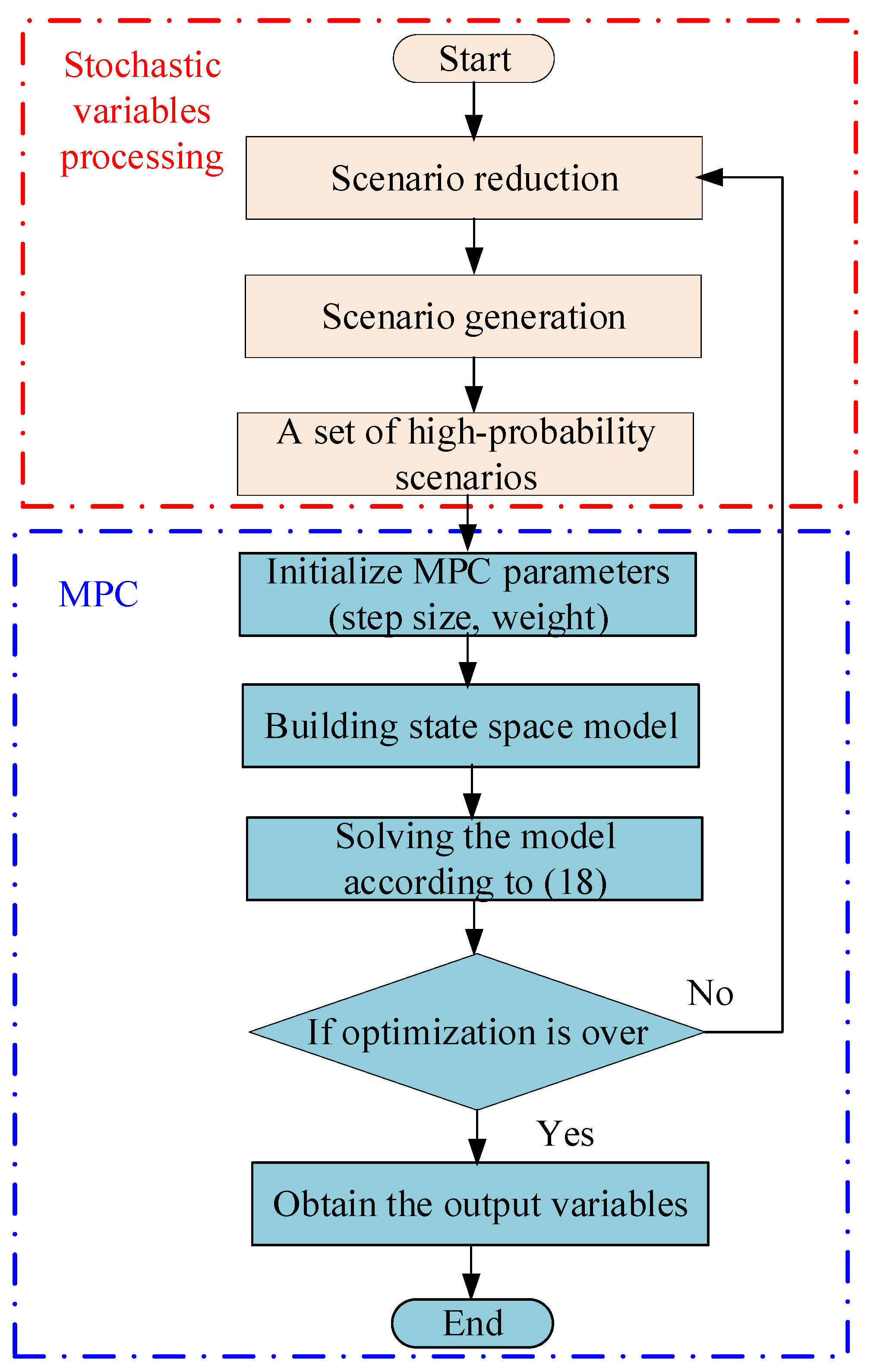
3.2. Lower-Layer Energy Management Strategy

Renewable energy and hydrogen loads have strong randomness. This randomness is prone to causing fluctuations in the power of the Elz and grid, leading to performance degradation or even damage to equipment. Therefore, it is necessary to control the disturbance of the renewable energy and hydrogen load.
The lower-layer energy management strategy considers the minute-level time scale and generates scheduling instructions every 15 min. The objective function is that the operation results of the lower layer track the scheduling results of the upper layer as much as possible, and minimize fluctuations of the Elz and the grid operating power. Compared with MPC, SMPC has a stronger ability to cope with the randomness of renewable energy and hydrogen load. Therefore, a solution algorithm based on SMPC is proposed to further optimize the operating state of equipment in this paper. The flow chart of the SMPC algorithm is shown in Figure 4, which mainly includes two parts: stochastic variables process and model predictive control.
The SMPC algorithm requires generating stochastic variable scenarios, which include hydrogen consumption and renewable energy power generation. Based on the distribution of prediction errors, a large number of scenarios of renewable energy power generation and hydrogen load are sampled to represent the variation characteristics of stochastic variables in each optimization cycle. Among the existing methods for scenario sampling, LHS provides better coverage of the space of random variables. Therefore this study chooses LHS to generate a large number of stochastic variable scenarios.
The specific steps of LHS are [26]:
(1)
Divide the sample into m equal probability distribution intervals;
(2)
Randomly select a point within the interval in (1);
(3)
Randomly combine the points obtained in (2) with other variables to obtain the sampling points xi, and obtain the sample values of the sampling points through the inverse transformation of the cumulative probability distribution function f (xi) = Pi.
Through LHS, corresponding m scenarios can be generated for photovoltaic power, wind power, and hydrogen load consumption with a probability of 1/m.
However, generating too many scenarios can easily affect computational speed. It is necessary to reduce scenarios to obtain a set of high-probability scenarios, and the system can be further optimized by using the reduced scenarios. The methods of scenario reduction mainly include forward selection and backward reduction. To improve computational efficiency, there are some improved scenario reduction methods, including fast forward selection and simultaneous backward reduction. This paper adopts the simultaneous backward reduction method to reduce scenarios at each time step in the control cycle. The principle is to filter one scenario each time and place it in the discarded set until the number of remaining scenarios equals the set value and it stops. The specific process is [27]:
Set the number of original scenarios to P and the number of reduced scenarios to M.
(1)
Set two specific scenarios at a certain time step as ai and aj, then calculate the probability distance d (ai, aj) of pairwise scenarios in the scenario set:
d ( a i , a j ) = P i ( a i a j ) 2
where Pi represents the probability of scenario I;
(2)
Delete the scenario with the smallest distance obtained in (1);
(3)
Modify the remaining number of scenarios P = P − 1 to ensure that the sum of probabilities for all scenarios is equal to 1, and add the probability of the deleted scenario to the nearest scenario;
(4)
Repeat the above steps at each time step until the number of scenarios reaches the set value M, and the probability of each scenario is εi.
MPC is essentially a multi-objective optimization problem. Firstly, a prediction model is used to predict the state of the system within the prediction step Np, and the Np value is set to 4. Common forms of prediction models include convolutional models, mechanical models, fuzzy models, neural networks, etc. Among them, the state space model of mechanism models is widely used, and the state space model can be expressed as follows [28]:
x ( k + 1 ) = A x ( k ) + B 1 u ( k ) + B 2 w ( k ) y ( k ) = C x ( k ) + D 1 u ( k ) + D 2 w ( k )
where x (k) represents the state variables, y (k) represents the output variables, u (k) represents the control variables, and w (k) represents the disturbance variables.
The state space model is established based on the model of the HFS equipment:
S O C ( t + 1 ) = S O C ( t ) + P bat ( t ) Δ T / E bat L O H ( t + 1 ) = L O H ( t ) + P ele Δ T η ele H H V m max + m off ( t ) Δ T m max m load ( t ) Δ T m max P bat ( t ) = P wt ( t ) + P pv ( t ) P grid ( t ) P com ( t ) P ele ( t )
Furthermore, the state variables choose [SOC(t), LOH(t)]T, control variables choose [Pgrid(t), Pele(t)]T, output variables choose [Pbat(t)]T, and disturbance variables choose [Ppv(t) + Pwt(t), mload(t)]T.
The prediction model can be used to obtain the value of the system state quantity at the next moment based on the current moment state. By solving through rolling optimization, the control sequence in the control cycle is obtained. Each time, the control sequence of the next time is obtained according to the control sequence of the current time, and then the rolling solution is used to obtain the control sequence for the entire optimization cycle.
The MPC objective function designed in this paper is divided into three parts:
(1)
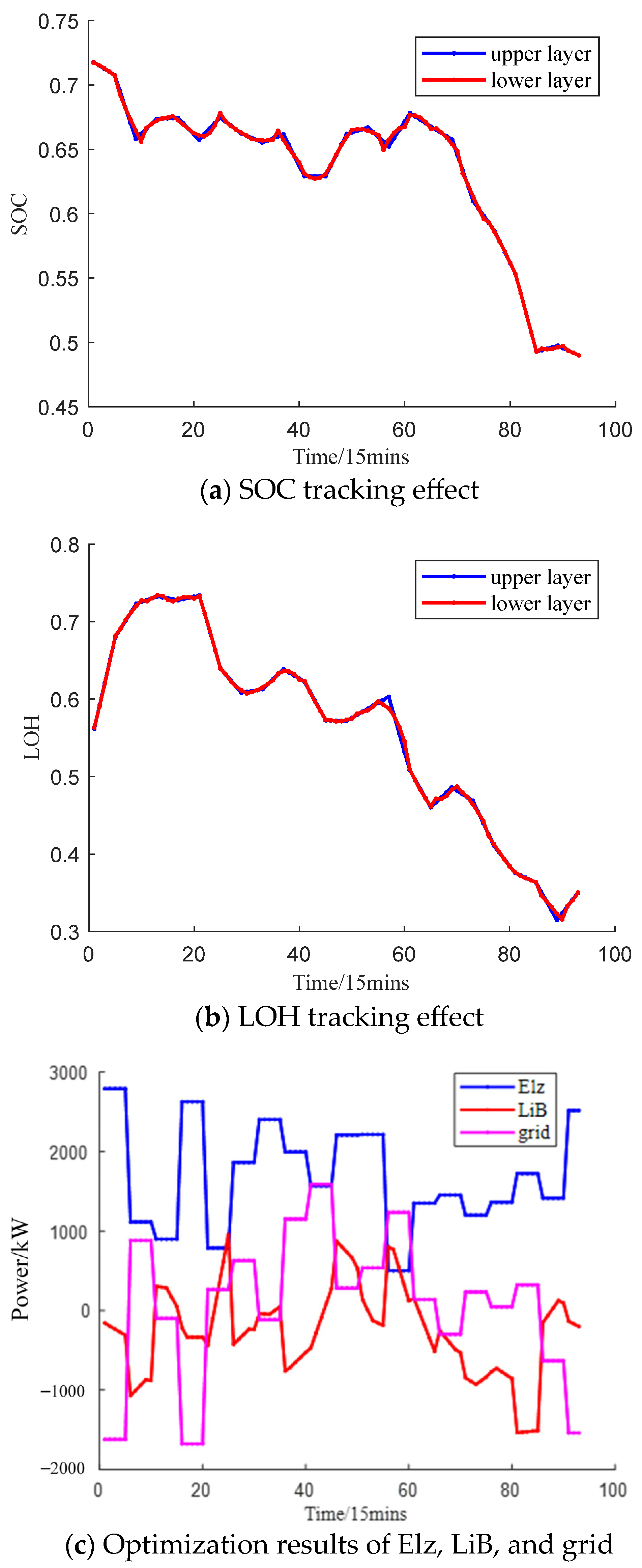
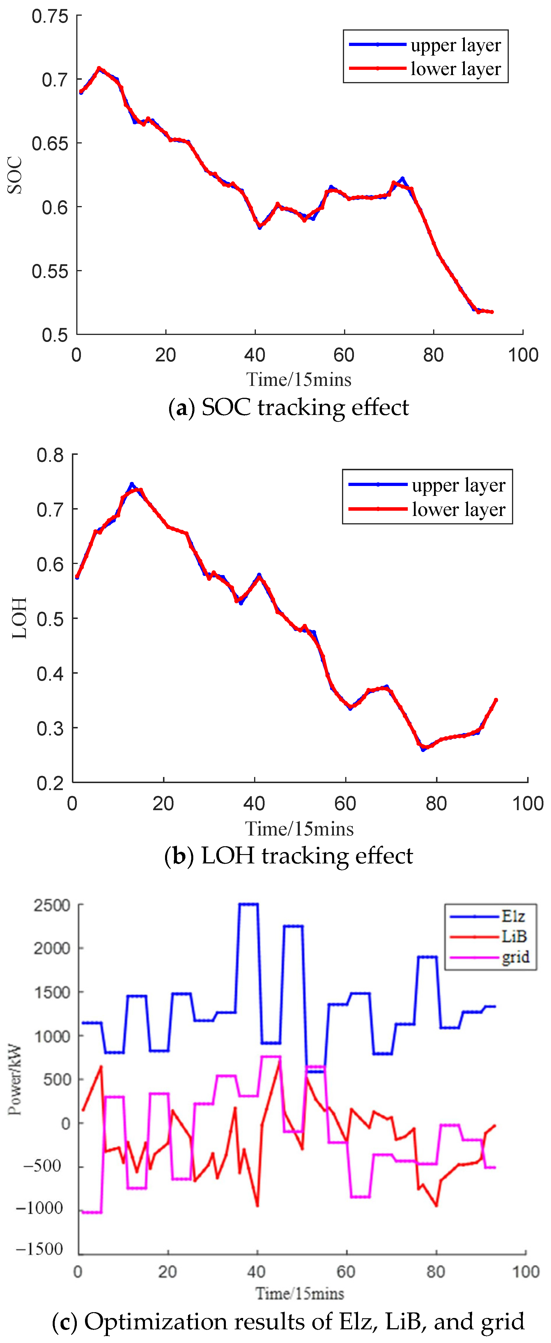
State variables SOC and LOH should track the optimization results of the upper-layer energy management as much as possible;
(2)
Minimize power fluctuations of the Elz and grid during each control cycle;
(3)
Introduce penalty factors, which allow the value of the state variables to exceed the limit, but still aim to minimize the exceeding value of the lower layer state variables as much as possible.
Based on the above goals, according to the principle of SMPC, the objective function is converted into the following form:
C lower = min i = 1 M ε i ( j + t ) ( j = 1 N p Q 1 ( S O C ( j + t ) S O C ref ( j + t ) ) 2 + Q 2 ( L O H ( j + t ) L O H ref ( j + t ) ) 2 + Q 3 ε 1 ( j + t ) + Q 4 ε 2 ( j + t ) + j = 0 N p 1 R 1 ( P ele ( j + t ) P ele ( j + t 1 ) 2 + R 2 ( P bat ( j + t ) P bat ( j + t 1 ) ) 2 )
Among them, SOCref and LOHref represent the results of SOC and LOH obtained from the upper layer, Q1, Q2, Q3, Q4, R1, and R2 represent the weight coefficients of SOC, LOH, penalty of exceeding the SOC limit, penalty of exceeding the LOH limit, Elz power fluctuation, and grid power fluctuation, respectively. Therefore, the stochastic problem can be transformed into a deterministic problem by introducing scenario probabilities within each time step to reduce the inference of random variables.
The constraints for lower layer energy management have two improvements compared with upper-layer energy management, and the other conditions are the same as those of the upper layer:
(1)
In the process of tracking state variables, the values of lower-layer state variables are likely to exceed the limit. Therefore, this paper introduces slack variables ε1 and ε2, which allows for a small amount of overstepping of the lower layer state variables:
S O C min ε 1 S O C ( t ) S O C max + ε 1 L O H min ε 2 L O H ( t ) L O H max + ε 2
(2)
In addition, the fluctuations of power need to meet the constraints:
Δ P elemin Δ P ele Δ P elemax Δ P gridmin Δ P grid Δ P gridmax
Among them, ΔPelemin, ΔPelemax, ΔPgridmin, and ΔPgridmax represent the minimum and maximum power fluctuations of the Elz, the minimum and maximum power fluctuations of the grid.
The results of the random variables are combined with the MPC to solve the objective function by transforming it into the form of Equation (18), which is a quadratic programming problem, and the quadratic programming problem is solved by invoking the quadprog solving environment through MATLAB2022a+Yalmip to complete the solution of the lower-layer energy management strategy.

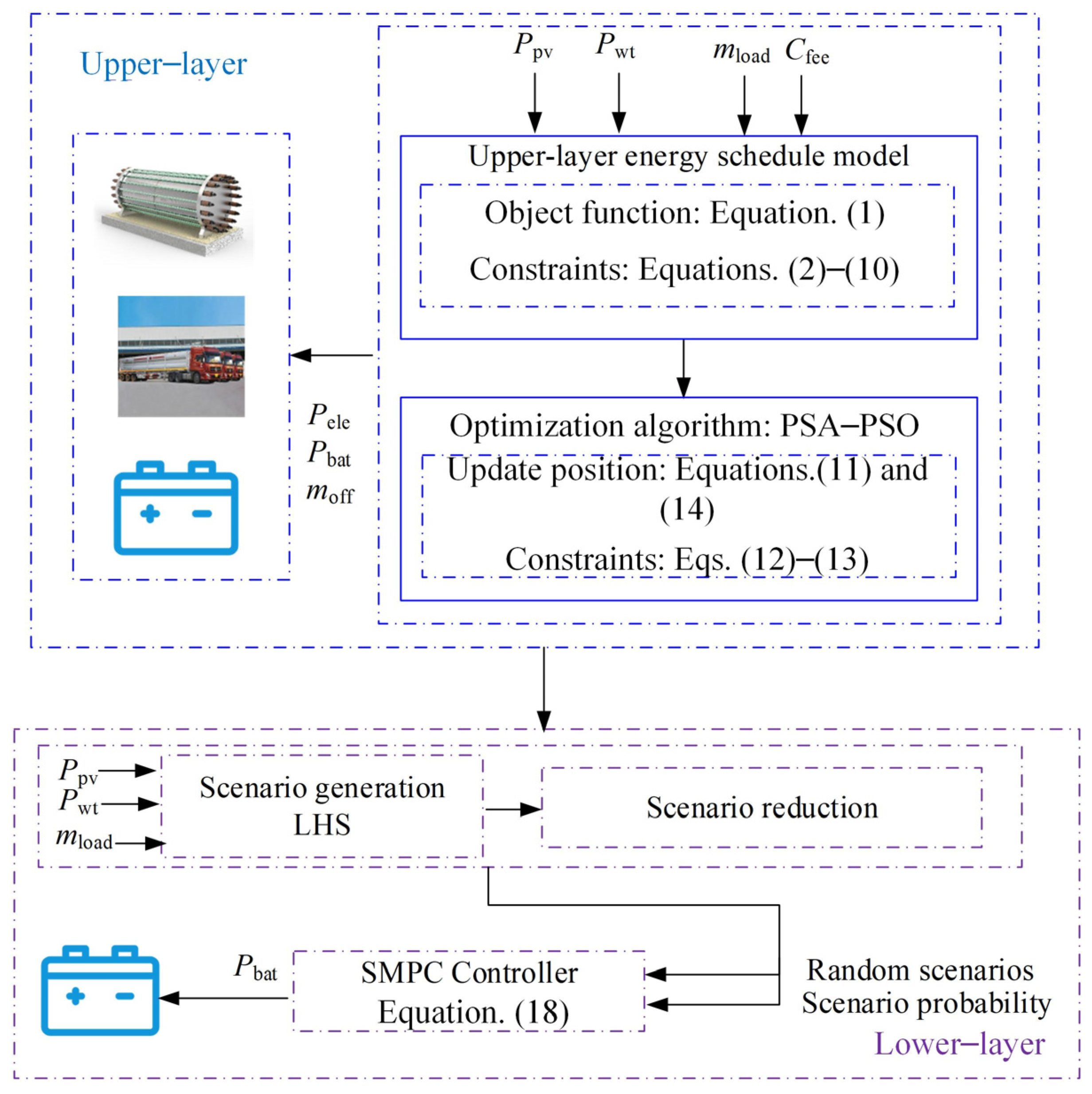
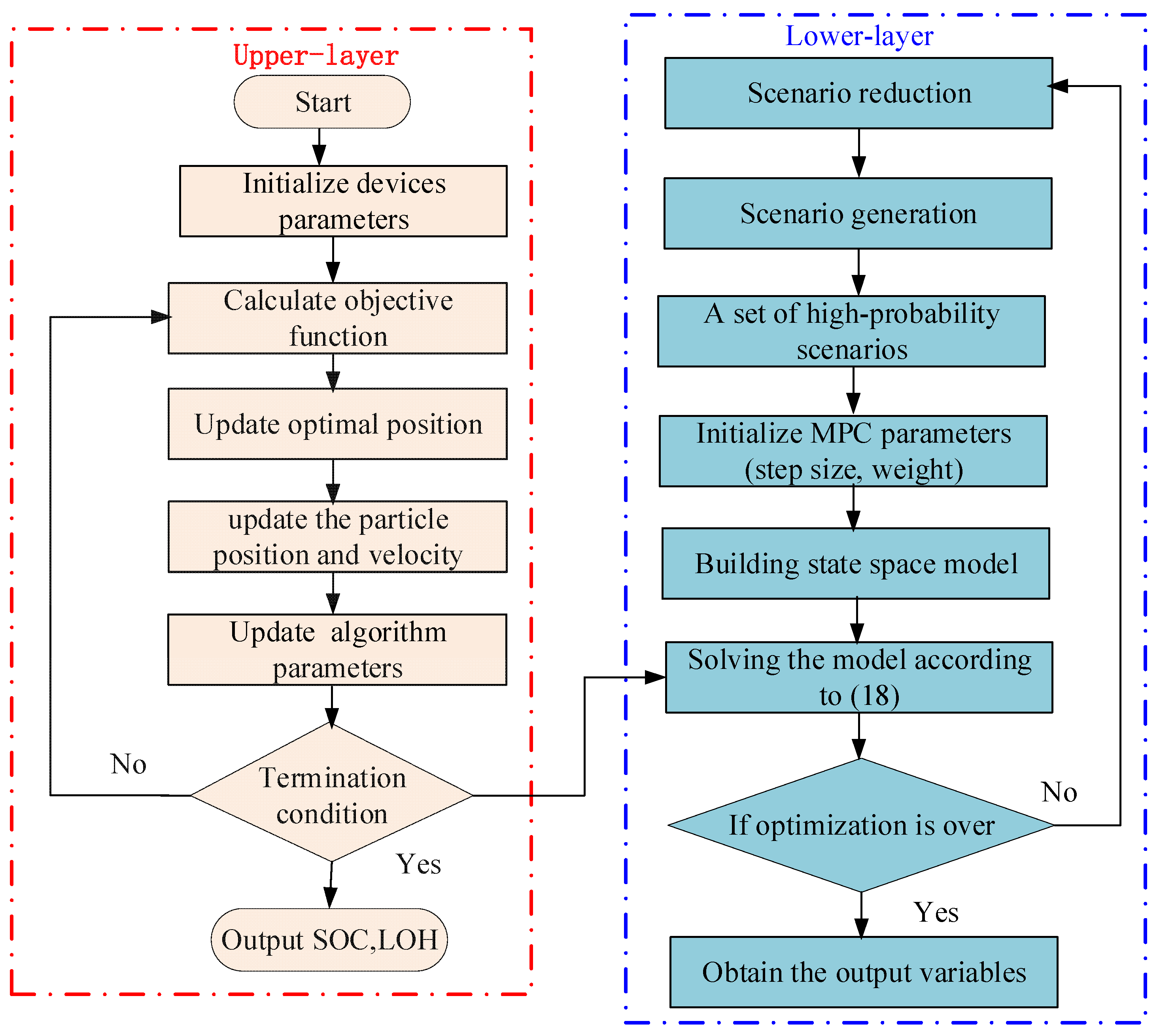
4. Multi-Time-Scale Energy Management Strategy Flow Chart

The flow chart of the multi-time scale energy management strategy for the port HFS proposed is shown in Figure 5:
The specific steps include:
(1)
Initialize PSA-PSO algorithm parameters and device parameters;
(2)
Each iteration of the upper layer energy management updates the speed and position according to Equations (11) and (14), and updates the algorithm parameters according to Equations (12) and (13) at the end of the iteration;
(3)
If the termination condition is met (the current iteration number reaches the maximum iteration number), SOC and LOH are output to complete the upper layer energy management algorithm solution. Otherwise, continue searching from (2) until the termination condition is met;
(4)
Stochastic variables (WT and PV power, and hydrogen load) are preprocessed by linear interpolation to meet the time scale requirements for lower-layer control;
(5)
A large amount of renewable energy power generation and hydrogen load consumption are obtained through LHS within the prediction step size;
(6)
Reduce scenarios at different time steps through the simultaneous backward reduction method and obtain the probability of the reduced scenarios;
(7)
Initialize the parameters of MPC, including prediction step size and weight coefficients;
(8)
Establish a state space model of HFS;
(9)
Combine the stochastic variable scenarios, corresponding probability values processed in (6) and the state variables input in (3), the MPC model is solved according to Equation (18);
(10)
When the optimization cycle ends, the solution is completed and Pbat is output. Otherwise, repeat (5)–(8) until the optimization cycle ends.

5. Guidelines for Graphics Preparation and Submission

To verify the effectiveness of the proposed energy management strategy with real data from an HFS in southern China, different scenarios of the HFS are selected for analysis. The predicted WT and PV power, hydrogen load consumption, and electricity price curves for the two scenarios are shown in Figure 6, Figure 7 and Figure 8.
The parameter settings are shown in Table 2 [29,30,31,32].
The optimization results of the upper-layer energy management strategies in different scenarios are shown in Figure 9 and Figure 10, respectively, and all the optimization results satisfy the constraints. The HFS achieves the local power balance by coordinating the LiB and the grid, and achieves the hydrogen demand of the local hydrogen load by coordinating the P2H link and the external hydrogen source with a certain margin of hydrogen in the hydrogen storage tank.
From Figure 9 and Figure 10, the operation of the HFS presents the following characteristics in different scenarios: (1) Most of the time, the grid is not needed to produce hydrogen. When there is insufficient hydrogen produced locally, it is mainly through the external transportation of hydrogen to satisfy the demand for hydrogen on that day. (2) The SOC overall changes in different scenarios are relatively small, and maintain the fluctuation in the range of 0.5–0.7. LiB is charged during the day and discharged at night, which is in line with the basic working mode of LiB. (3) LOH will be less than 0.5 for a relatively long period of time, and will change abruptly at the last moment to meet the LOH constraints at the last moment, which is relatively obvious in Scenario 1, and it is mainly achieved by increasing the power of Elz to affect the amount of hydrogen production.
The optimization results of the proposed algorithm are compared with four traditional algorithms: genetic algorithm (GA), particle swarm algorithm (PSO), firefly algorithm (FA), and fruit fly algorithm (FOA). A comparison of fitness curves for different algorithms in different scenarios is shown in Figure 11. The cost optimization results and convergence speed of different algorithms are shown in Table 3. From the graph and table, some algorithms have faster convergence speeds; however, they exhibit premature phenomena (FA, FOA), making it difficult to obtain global optimal values. Although some algorithms keep trying to avoid premature phenomena, they have a longer number of iterations still failing to reach the local optimum (PSO and GA). The PSA-PSO algorithm proposed achieved good optimization results.
Sensitivity analysis of upper-layer optimization is conducted by constructing scenarios of hydrogen price and electricity price changes based on the predicted value of renewable energy and hydrogen load as the fixed output in different scenarios. The analysis results are shown in Table 4 (F1: original scenario, F2: changing hydrogen price, F3: changing valley time electricity price, F4: changing flat time electricity price, and F5: changing peak time electricity price). From this table, the flat time electricity price is the most sensitive input factor in scenario 1, while hydrogen price is the most sensitive input factor in scenario 2. Since the volatility of the hydrogen load in scenario 2 is stronger than that in scenario 1, the hourly supply of hydrogen from external sources to meet the hydrogen load supply demand is relatively more volatile. For this reason, the price of the external hydrogen source has a more pronounced sensitivity in scenario 2.
Different operating scenarios of lower-layer energy management by the SMPC algorithm are shown in Figure 12 and Figure 13. Firstly, stochastic variables are sampled using LHS. This paper sets 400 scenarios for WT power, PV power, and hydrogen consumption, then reduces them to 2 scenarios at each time step within the control cycle using the simultaneous backward reduction method. Finally, the reduced scenarios are brought into the objective function to convert the stochastic problem into a deterministic problem. From the figures, it can be seen that the SMPC algorithm can make the power fluctuations of the Elz and grid very small during each control cycle and has a good tracking effect on the upper SOC and LOH.
Compare the SMPC algorithm with two MPC algorithms: MPC1 (using real values of stochastic variables) and MPC2 (using predicted values of stochastic variables). To quantify the optimization effect more intuitively, the average fluctuation power Pflu is introduced to compare the control effect [33]:
P fluave = 1 m i = 1 m P lower ( i ) P ref ( i )
where Plower represents the power control results of the lower layer SMPC and MPC2 algorithms, Pref represents the power control results of the MPC1 algorithm, and m1 represents the number of control times.
The control results of different MPC algorithms in different scenarios are shown in Figure 14 and Figure 15, and the Pflu results are shown in Table 5 and Table 6. SMPC has a strong ability to cope with stochastic variables in different scenarios, thus making the control results closer to the real values.

6. Conclusions

A multi-time-scale hierarchical energy management strategy for integrated production, storage, and supply HFS is proposed. The following conclusions can be drawn:
(1)
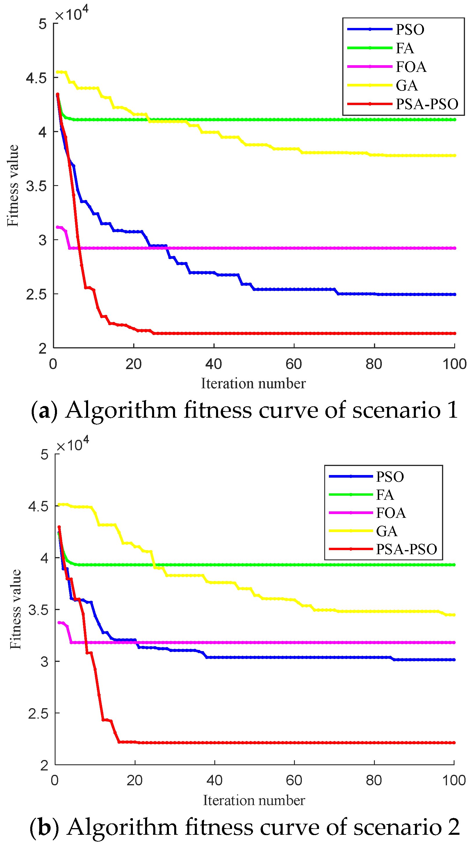
Aiming at the economic issues of HFSs, the upper layer of the proposed strategy is on an hourly level, and the optimization goal is to minimize the sum of equipment operation and maintenance costs, electricity purchase cost, and hydrogen purchase cost. Aiming at the problems of the PSO algorithm, including being prone to local optimal value and slow convergence speed, a PSA-PSO algorithm is proposed to solve those problems. This algorithm introduced Gaussian disturbance with adaptive adjustment of the learning factor, inertia weight, and disturbance step size to improve solution accuracy and convergence speed.
(2)
Aiming at the randomness of renewable energy and hydrogen load, the lower layer is at the minute-level time scale. To address the disturbance caused by the randomness of the renewable energy and hydrogen load on the system, the SMPC algorithm is proposed. The LHS and simultaneous backward reduction method have been used to generate and reduce stochastic variables to obtain a set of high-probability scenarios, which have been brought into the MPC to suppress the interference of stochastic variables on the operation of HFS.
(3)
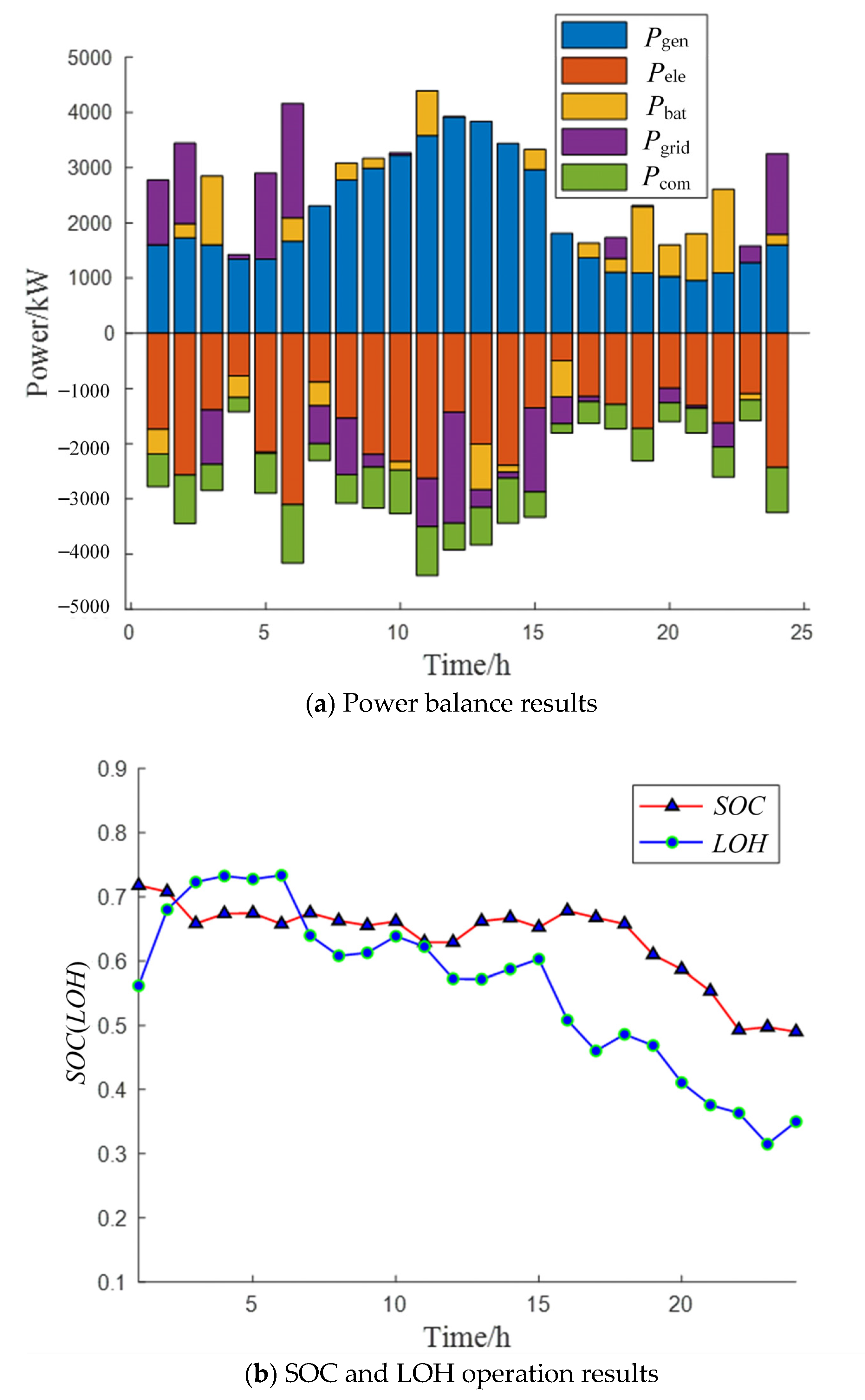
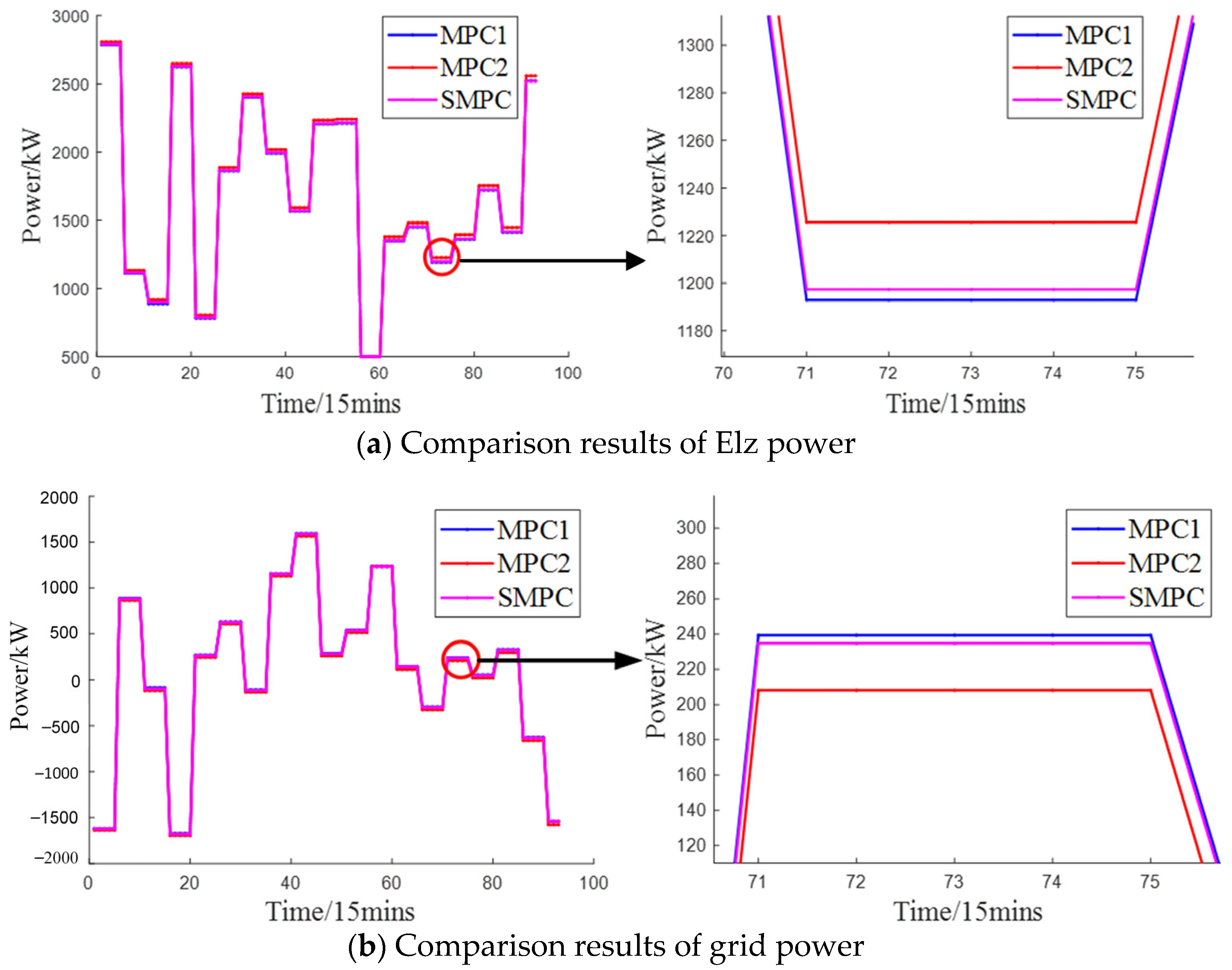
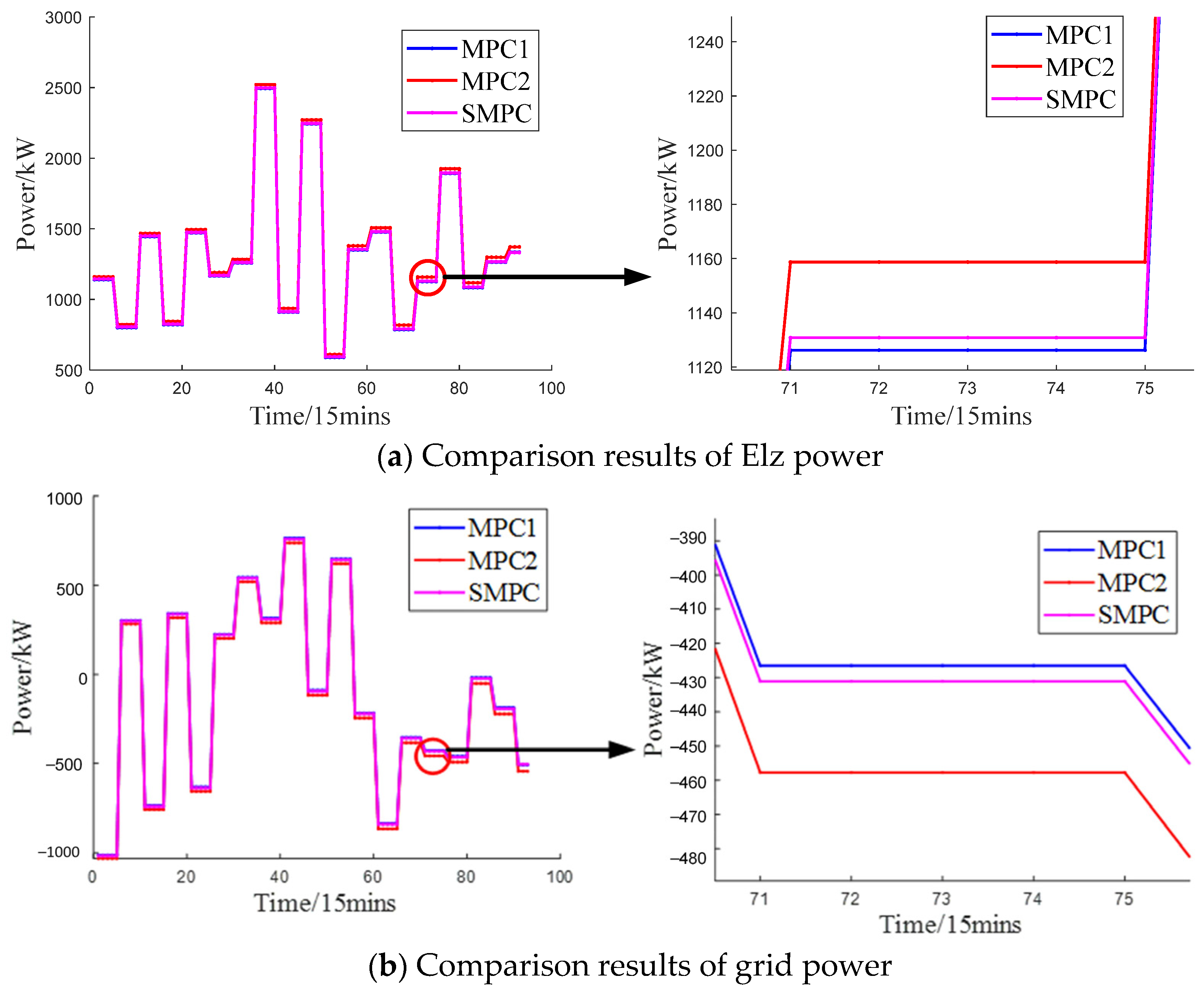
Operation data from southeastern China were used for example analysis. The results show that the proposed PSA-PSO algorithm can better balance the characteristics of fast convergence speed and good optimization effect compared with traditional optimization algorithms, such as PSO, FA, FOA, and GA. The daily operation cost solved by PSA-PSO can be reduced by up to 16,460 ¥ and 17,170 ¥ in different scenarios. The proposed SMPC algorithm can significantly reduce with the inference of renewable energy and hydrogen load to Elz and grid compared with the traditional MPC algorithm. Compared with the traditional MPC algorithm, the Pflu of Elz in different scenarios was reduced by 16.2% and 14.9%, the Pflu of grid in different scenarios was reduced by 17.2% and 15.9%.
(4)
Regarding future work, the large-capacity electrolytic hydrogen production model is a simple electrochemical empirical model, and it is necessary to establish a large-capacity electrolytic cell model that considers the deep coupling of energy–material flow to comprehensively reflect the energy change and material transfer laws of electrolytic hydrogen production equipment under different working conditions. The refined energy management strategy is verified using equipment from an actual HFS in Zhoushan Port, Ningbo, Zhejiang Province, China.

Author Contributions

Conceptualization, Z.J.; Methodology, R.L.; Software, W.G. and L.X.; Validation, C.S.; Formal analysis, J.Y. All authors have read and agreed to the published version of the manuscript.

Funding

Supported by Research Project of China Yangtze Power Co., Ltd. (Project number: 1523020038/6123020003; Contract No.: Z152302045/Z612302015).

Data Availability Statement

The original contributions presented in the study are included in the article, further inquiries can be directed to the corresponding author.

Conflicts of Interest

Author Zhuoyu Jiang, Rujie Liu and Lei Xiong were employed by the company Three Gorges Electric Energy Co., Ltd., and Author Weiwei Guan was employed by the company China Yangtze power Co., Ltd. The remaining authors declare that the research was conducted in the absence of any commercial or financial relationships that could be construed as a potential conflict of interest.

References

  1. Ma, N.; Zhao, W.; Wang, W.; Li, X.; Zhou, H. Large scale of green hydrogen storage: Opportunities and challenges. Int. J. Hydrogen Energy 2024, 50, 379–396. [Google Scholar] [CrossRef]
  2. Iris, Ç.; Lam, J.S.L. A review of energy efficiency in ports: Operational strategies, technologies and energy management systems. Renew. Sustain. Energy Rev. 2019, 112, 170–182. [Google Scholar] [CrossRef]
  3. Apostolou, D.; Xydis, G. A literature review on hydrogen refuelling stations and infrastructure. Current status and future prospects. Renew. Sustain. Energy Rev. 2019, 113, 109292. [Google Scholar] [CrossRef]
  4. Hossain, A.; Islam, R.; Hossain, A.; Hossain, M. Control strategy review for hydrogen-renewable energy power system. J. Energy Storage 2023, 72, 108170. [Google Scholar] [CrossRef]
  5. Van, L.P.; Chi, K.D.; Duc, T.N. Review of hydrogen technologies based microgrid: Energy management systems, challenges and future recommendations. Int. J. Hydrogen Energy 2023, 48, 14127–14148. [Google Scholar] [CrossRef]
  6. Tostado-Véliz, M.; Ghadimi, A.A.; Miveh, M.R.; Bayat, M.; Jurado, F. Uncertainty-aware energy management strategies for PV-assisted refuelling stations with onsite hydrogen generation. J. Clean. Prod. 2022, 365, 132869. [Google Scholar] [CrossRef]
  7. Shams, M.H.; Niaz, H.; Liu, J.J. Energy management of HFSs in a distribution system: A bilevel chance-constrained approach. J. Power Sources 2022, 533, 231400. [Google Scholar] [CrossRef]
  8. Abomazid, A.M.; El-Taweel, N.A.; Farag, H.E.Z. Optimal Energy Management of Hydrogen Energy Facility Using Integrated Battery Energy Storage and Solar Photovoltaic Systems. IEEE Trans. Sustain. Energy 2022, 13, 1457–1468. [Google Scholar] [CrossRef]
  9. Pang, Y.; Pan, L.; Zhang, J.; Chen, J.; Dong, Y.; Sun, H. Integrated sizing and scheduling of an off-grid integrated energy system for an isolated renewable energy HFS. Appl. Energy 2022, 323, 119573. [Google Scholar] [CrossRef]
  10. Dadkhah, A.; Bozalakov, D.; De Kooning, J.D.M.; Vandevelde, L. On the optimal planning of a hydrogen refuelling station participating in the electricity and balancing markets. Int. J. Hydrogen Energy 2021, 46, 1488–1500. [Google Scholar] [CrossRef]
  11. Zhang, W.; Maleki, A.; Nazari, M.A. Optimal operation of a hydrogen station using multi-source renewable energy (solar/wind) by a new approach. J. Energy Storage 2022, 53, 104983. [Google Scholar] [CrossRef]
  12. Erdinç, F.G.; Çiçek, A. Cost minimization oriented energy management of PV-assisted refueling and recharging stations for FC-ultracapacitor hybrid trams. Energy Convers. Manag. 2023, 287, 117103. [Google Scholar] [CrossRef]
  13. Liu, L.; Su, X.; Chen, L.; Wang, S.; Li, J.; Liu, S. Elite Genetic Algorithm Based Self-Sufficient Energy Management System for Integrated Energy Station. IEEE Trans. Ind. Applicat. 2024, 60, 1023–1033. [Google Scholar] [CrossRef]
  14. Jordehi, A.R.; Mansouri, S.A.; Tostado-Veliz, M.; Safaraliev, M.; Hakimi, S.M.; Nasir, M. A tri-level stochastic model for operational planning of microgrids with hydrogen refuelling station-integrated energy hubs. Int. J. Hydrogen Energy 2024, 96, 1131–1145. [Google Scholar] [CrossRef]
  15. Fang, X.; Wang, Y.; Dong, W.; Yang, Q.; Sun, S. Optimal energy management of multiple electricity-hydrogen integrated charging stations. Energy 2023, 262, 125624. [Google Scholar] [CrossRef]
  16. Rahbar, K.; Xu, J.; Zhang, R. Real-Time Energy Storage Management for Renewable Integration in Microgrid: An Off-Line Optimization Approach. IEEE Trans. Smart Grid 2015, 6, 124–134. [Google Scholar] [CrossRef]
  17. Velarde, P.; Valverde, L.; Maestre, J.; Ocampo-Martinez, C.; Bordons, C. On the comparison of stochastic model predictive control strategies applied to a hydrogen-based microgrid. J. Power Sources 2017, 343, 161–173. [Google Scholar] [CrossRef]
  18. Ahmad, S.; Shafiullah, M.; Ahmed, C.B.; Alowaifeer, M. A Review of Microgrid Energy Management and Control Strategies. IEEE Access 2023, 11, 21729–21757. [Google Scholar] [CrossRef]
  19. Vivas, F.J.; De Las Heras, A.; Segura, F.; Andújar, J.M. A review of energy management strategies for renewable hybrid energy systems with hydrogen backup. Renew. Sustain. Energy Rev. 2018, 82, 126–155. [Google Scholar] [CrossRef]
  20. Haider, S.A.; Sajid, M.; Iqbal, S. Forecasting hydrogen production potential in islamabad from solar energy using water electrolysis. Int. J. Hydrogen Energy 2021, 46, 1671–1681. [Google Scholar] [CrossRef]
  21. Eichman, J.; Harrison, K.; Peters, M. Novel Electrolyzer Applications: Providing More Than Just Hydrogen; No. NREL/TP-5400-61758; National Renewable Energy Lab.: Golden, CO, USA, 2014; Volume 61758, p. 1159377. [Google Scholar] [CrossRef]
  22. Zhang, Y.; Campana, P.E.; Lundblad, A.; Yan, J. Comparative study of hydrogen storage and battery storage in grid connected photovoltaic system: Storage sizing and rule-based operation. Appl. Energy 2017, 201, 397–411. [Google Scholar] [CrossRef]
  23. Hu, S.; Guo, B.; Ding, S.; Yang, F.; Dang, J.; Liu, B.; Gu, J.; Ma, J.; Ouyang, M. A comprehensive review of alkaline water electrolysis mathematical modeling. Appl. Energy 2022, 327, 120099. [Google Scholar] [CrossRef]
  24. Ahangar, H.G.; Yew, W.K.; Flynn, D. Smart Local Energy Systems: Optimal Planning of Stand-Alone Hybrid Green Power Systems for On-Line Charging of Electric Vehicles. IEEE Access 2023, 11, 7398–7409. [Google Scholar] [CrossRef]
  25. Li, S.-B.; Kang, Z.-T. Capacity Optimization of Clean Renewable Energy in Power Grid Considering Low Temperature Environment Constraint. IEEE Access 2022, 10, 2740–2752. [Google Scholar] [CrossRef]
  26. Wang, D.; Fu, C.; Zhao, Q.; Hu, T. A PSO-Based Optimization Design of W-Type Noncontact Transformer for Stable Power Transfer in DWPT System. IEEE Trans. Ind. Appl. 2022, 58, 1211–1221. [Google Scholar] [CrossRef]
  27. Growe-Kuska, N.; Heitsch, H.; Romisch, W. Scenario reduction and scenario tree construction for power management problems. In Proceedings of the 2003 IEEE Bologna Power Tech Conference Proceedings, Bologna, Italy, 23–26 June 2003; Volume 3, p. 7. [Google Scholar] [CrossRef]
  28. He, J.; Shi, C.; Wei, T.; Jia, D. Stochastic Model Predictive Control of Hybrid Energy Storage for Improving AGC Performance of Thermal Generators. IEEE Trans. Smart Grid 2022, 13, 393–405. [Google Scholar] [CrossRef]
  29. Gennitsaris, S.G.; Kanellos, F.D. Emission-Aware and Cost-Effective Distributed Demand Response System for Extensively Electrified Large Ports. IEEE Trans. Power Syst. 2019, 34, 4341–4351. [Google Scholar] [CrossRef]
  30. Garcia-Torres, F.; Vilaplana, D.G.; Bordons, C.; Roncero-Sanchez, P.; Ridao, M.A. Optimal Management of Microgrids with External Agents Including Battery/Fuel Cell Electric Vehicles. IEEE Trans. Smart Grid 2019, 10, 4299–4308. [Google Scholar] [CrossRef]
  31. Huang, W.; Zhang, B.; Ge, L.; He, J.; Liao, W.; Ma, P. Day-ahead optimal scheduling strategy for electrolytic water to hydrogen production in zero-carbon parks type microgrid for optimal utilization of electrolyzer. J. Energy Storage 2023, 68, 107653. [Google Scholar] [CrossRef]
  32. Wang, S.; Kong, L.; Liu, C.; Cai, G. MPC-based energy optimization and regulation for zero-carbon energy supply building. Int. J. Hydrogen Energy 2024, 82, 1196–1210. [Google Scholar] [CrossRef]
  33. He, J.; Shi, C.; Wei, T.; Peng, X.; Guan, Y. Hierarchical optimal energy management strategy of hybrid energy storage considering uncertainty for a 100% clean energy town. J. Energy Storage 2021, 41, 102917. [Google Scholar] [CrossRef]
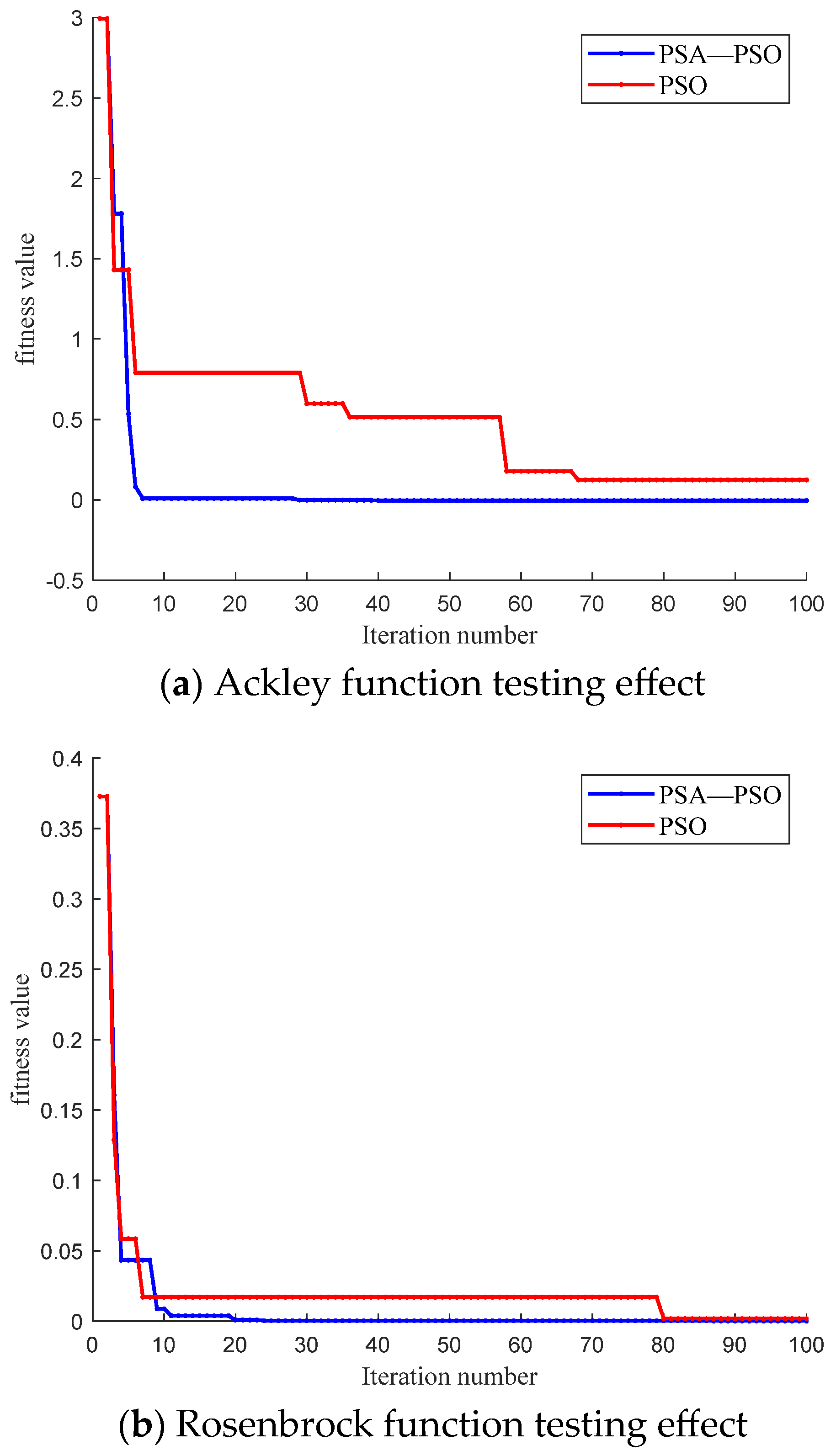
Figure 1. Structure of integrated green hydrogen production, storage, and supply HFS.
Energies 18 01583 g001
Figure 2. Principle of multi-time scale energy management strategy for port HFS.
Energies 18 01583 g002
Figure 3. PSA–PSO algorithm testing results under different test functions.
Energies 18 01583 g003
Figure 4. Flow chart of SMPC algorithm.
Energies 18 01583 g004
Figure 5. Flow chart of multi-time-scale energy management strategy.
Energies 18 01583 g005
Figure 6. Daily predicted wind and photovoltaic power generation curves.
Energies 18 01583 g006
Figure 7. Daily predicted hydrogen load curves.
Energies 18 01583 g007
Figure 8. Daily electricity price curve.
Energies 18 01583 g008
Figure 9. Upper–layer optimization results (scenario 1).
Energies 18 01583 g009aEnergies 18 01583 g009b
Figure 10. Upper–layer optimization results (scenario 2).
Energies 18 01583 g010aEnergies 18 01583 g010b
Figure 11. Fitness curves of different algorithms.
Energies 18 01583 g011
Figure 12. SMPC optimization results of scenario 1.
Energies 18 01583 g012
Figure 13. SMPC optimization results of scenario 2.
Energies 18 01583 g013
Figure 14. Control effect of different MPC (scenario 1).
Energies 18 01583 g014
Figure 15. Control effect of different MPCs (scenario 2).
Energies 18 01583 g015
Table 1. Comparison of the results of the two algorithms under different test functions.
Test FunctionAlgorithmOptimal ResultReal Optimal Result
AckleyPSO0.12380
PSA-PSO−0.00540
RosenbrockPSO0.00180
PSA-PSO0.00040
Table 2. Parameter settings of example analysis.
Parameters (Unit)Value
HHV (kWh/Kg)39.7
ηele0.7
Upper and lower limits of SOC0.9, 0.1
Upper and lower limits of LOH0.8, 0.2
Upper and lower limits of Elz power (KW)5000, 500
Upper and lower limits of LiB power (KW)−2000, 2000
LiB capacity (kWh)20,000
Mass of hydrogen storage tank (Kg)450
Operation and maintenance coefficients Elz and LiB (¥/KW)0.1, 0.1
Hydrogen price (¥/Kg)40
Upper and lower limits of grid power (KW)5000, −5000
Upper and lower limits of Elz power fluctuation (KW)−50, 50
Upper and lower limits of grid power fluctuation (KW)−50, 50
Weight of state variables Q1, Q21, 10
Weight of control variables R1, R210, 1
Weight of penalty variables Q3, Q480,000, 10,000
Table 3. Comparison of the effects of different algorithms.
AlgorithmCost (Scenario 1)/¥Cost (Scenario 2) /¥Convergence Speed (Scenario 1)Convergence Speed (Scenario 2)
GA37,79934,4708399
FOA29,12831,80044
FA41,09539,30856
PSO24,93930,1378285
PSA-PSO21,33922,1382521
Table 4. Sensitivity analysis results.
Scenario NameCost (Scenario 1)/¥Cost (Scenario 2)/¥
F221,33922,138
F320,31420,048
F422,68821,799
F422,81522,609
F521,53421,342
Table 5. Comparison results of MPC and SMPC (scenario 1).
AlgorithmElz Power Pflu/KWGrid Power Pflu/KW
MPC226.7325.85
SMPC22.3921.40
Table 6. Comparison results of MPC and SMPC (scenario 2).
AlgorithmElz Power Pflu/KWGrid Power Pflu/KW
MPC227.8626.85
SMPC23.7122.58
Disclaimer/Publisher’s Note: The statements, opinions and data contained in all publications are solely those of the individual author(s) and contributor(s) and not of MDPI and/or the editor(s). MDPI and/or the editor(s) disclaim responsibility for any injury to people or property resulting from any ideas, methods, instructions or products referred to in the content.

