Article

A Dynamic Power Flow Calculation Method for the “Renewable Energy–Power Grid–Transportation Network” Coupling System

1
State Grid Sichuan Electric Power Company, Chengdu 610041, China
2
State Grid Sichuan Economic Research Institute, Chengdu 610041, China
3
School of Electrical Engineering, Southwest Jiaotong University, Chengdu 610032, China
*
Author to whom correspondence should be addressed.
Energies 2025, 18(7), 1567; https://doi.org/10.3390/en18071567
Submission received: 20 February 2025 / Revised: 18 March 2025 / Accepted: 19 March 2025 / Published: 21 March 2025
(This article belongs to the Section F: Electrical Engineering)

Abstract

:
To address the issue of inaccurate power flow calculations in the asymmetric coupling system of a power grid and traction network, this paper proposes a dynamic power flow calculation method for the “renewable energy–power grid–transportation network” asymmetric coupled system. First, by utilizing the asymmetric characteristics of the traction transformer, the dynamic asymmetric nodal admittance matrix for the “renewable energy–power grid–transportation network” coupled system is established, which facilitates the construction of the mixed power flow equations for the coupling of the power grid and transportation network. Next, when analyzing the asymmetric coupling system of renewable energy, power grid, and transportation network in mountainous areas, it is necessary to allocate the power of electric multiple units (EMUs) to the three-phase (A, B, C) power distribution. To address this, a three-phase power balancing strategy is proposed, incorporating both the single-phase loads of EMUs and the output of renewable energy sources. Thus, a three-phase power balance strategy is proposed, incorporating the single-phase load of traction load units and renewable energy output. Finally, a simulation study is conducted using a real system of a regional power grid and traction network as a case example, demonstrating the suitability and effectiveness of the proposed model.

1. Introduction

In regional power grids with large-scale traction loads, such as those along mountainous railways, a coupled system naturally forms between the power grid and the traction network, as illustrated in Figure 1. In the figure, the layers of the power grid and traction network can be easily distinguished, with coupling achieved through traction transformers. With the integration of additional renewable energy sources into the power grid, a coupled renewable energy–power grid–transportation network system is formed, hereinafter referred to as the coupled system. Within this coupled system, the positions of the traction load change continuously over time, leading to variations in the system’s nodal admittance matrix. Furthermore, both the power output of the traction load and the output of renewable energy fluctuate over time. These cause the system power flow to constantly change dynamically. Consequently, the power flow calculations for the “renewable energy–power grid–transportation network” coupled system are of paramount importance for the dynamic characteristics and planning of the system.
The power flow calculations in traditional power systems have reached a highly mature level, encompassing classic methods such as the Newton–Raphson algorithm, PQ decomposition method, Gauss–Seidel algorithm, and the recently proposed holomorphic embedding method [1,2,3,4]. However, because the traction loads associated with traction load are single-phase loads and the power system operates as a three-phase system, these methods cannot be directly applied to traction power supply systems. To apply the aforementioned methods for power flow calculations in traction power supply systems, an equivalent transformation of the traction power system is required.
In addressing the power flow calculations for traction power supply systems, the sequential linear power flow method (SLPFM) is commonly employed to solve the current source iterative model [5,6,7,8,9]. Reference [6] treats the train as a power source, utilizing the train’s power to determine the train current, and subsequently applies SLPFM to only invert the nodal admittance matrix once at each simulation time step. Reference [8] constructed a unified mathematical model of the traction network, using a chain circuit model based on the transformation between three-phase and two-phase systems, taking into account the mutual influence between adjacent supply arms. Reference [9] describes the train drive system as a parallel static load model of an induction motor to perform power flow calculations for traction power supply systems based on train–network coupling. Reference [10] conducts power flow calculations for the train power source iterative model, using methods such as forward–backward substitution algorithms and the Newton–Raphson (NR) method based on the equivalent circuit of the traction network, which requires line merging or equivalent transformations when the traction network is complex. Reference [11] applies an improved PQ decomposition method to power flow calculations in traction power supply systems under direct supply, noting the challenges of decoupling lines in complex traction networks. The authors of [12] built a spatial state model of a fully parallel AT power supply system based on a chain network, useful for simulating steady-state and transient processes. Reference [13] proposes a power flow calculation method for the traction network based on a multi-port Thevenin equivalent circuit, which effectively enhances calculation speed compared to SLPFM. Reference [14] treats the entire AT traction network as a generalized node to perform power flow calculations using the NR method. These studies typically equate external power sources, focusing primarily on the modeling of the traction power supply system. Reference [15] further considers scenarios with multiple loads at the point of common coupling (PCC). Moreover, references [16,17,18,19] have applied SLPFM to harmonic power flow calculations in traction power systems. Reference [20] proposes a rapid power flow algorithm for traction power supply systems based on nodal analysis.
In summary, the existing models for traction power supply systems are predominantly based on current-type iterative models, which are unable to manage PV nodes within the power system. Generally, the upper-level grid is simplified as a slack node, making it impossible to conduct power flow calculations for asymmetric coupled systems between the power grid and traction network. And existing models cannot effectively deal with the “renewable energy–power grid–transportation network” power balance problem.
To address this issue, this paper proposes a dynamic power flow calculation method for the “renewable energy–power grid–transportation network” asymmetric coupled system, with the following main contributions:
  • Utilizing the asymmetric characteristics of traction transformers, a dynamic asymmetric nodal admittance matrix for the “renewable energy–power grid–transportation network” coupled system is established.
  • A three-phase power balance strategy that considers the single-phase loads of the traction load units and the output of renewable energy sources is proposed.
  • The dynamic power flow characteristics of the “renewable energy–power grid–transportation network” coupled system and the mutual influence between the renewable energy sources and traction load units are analyzed.

2. Construction of Dynamic Admittance Matrix for the “Renewable Energy–Power Grid–Transportation Network” Coupled System

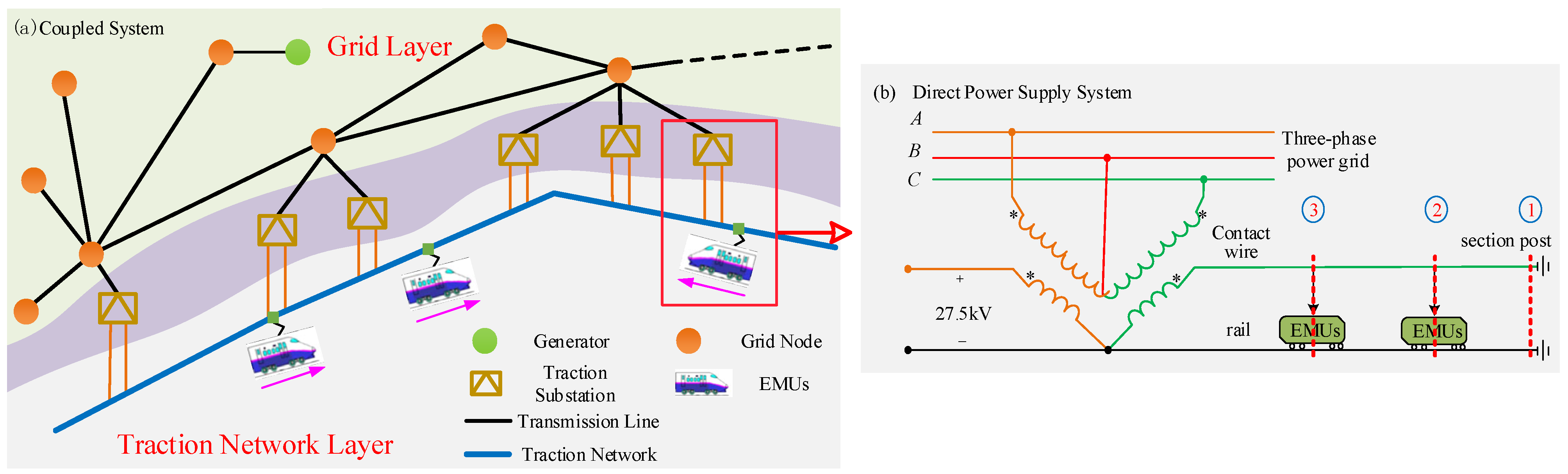
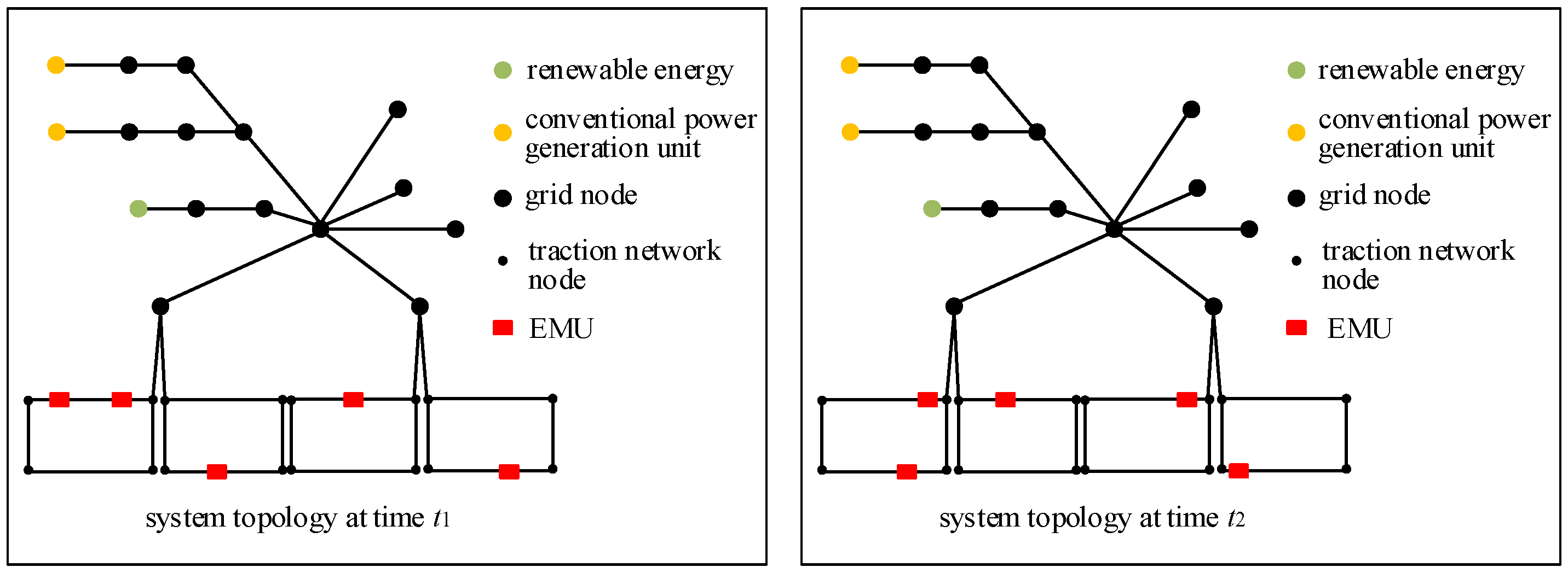
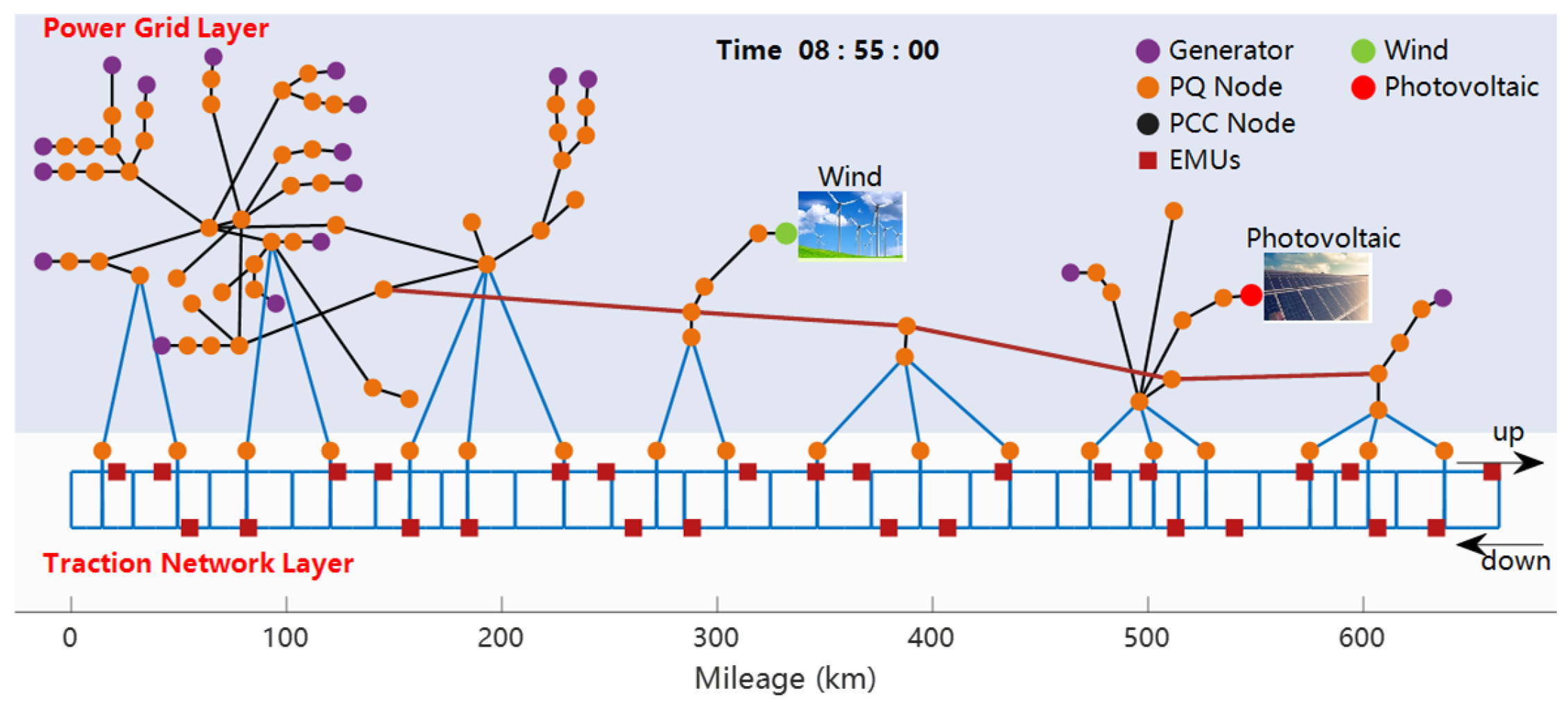
2.1. Construction of Dynamic Topological Structure for the Coupled System

The topology of a power system is naturally formed, with transmission lines serving as branches and power plants, traction substations, and loads acting as nodes. However, in traction power supply systems, due to the continuous movement of the EMUs, the topology is dynamically time-varying. A conventional approach to establishing such a topology is to consider each EMUs as a node and sectioning post as a single node. In the direct power supply system shown in Figure 2b, two EMUs operate on the right feeding arm, including one sectioning post, hence forming a chain structure with three nodes. The chain structure model is illustrated in Figure 3, where the locations of EMUs, AT substations, and sectioning posts (nodes) can be regarded as cross-sectional planes, with EMUs considered as loads.
Based on the above analysis, Figure 4 presents the topology of the coupled system composed of the local power grid and two traction substations at times t1 and t2, represented in the form of nodes and branches. When the EMUs are in operation, this topology varies with the position of the EMUs, forming a dynamic topology.
The dynamic nodal admittance matrix of the coupled system will be established below.

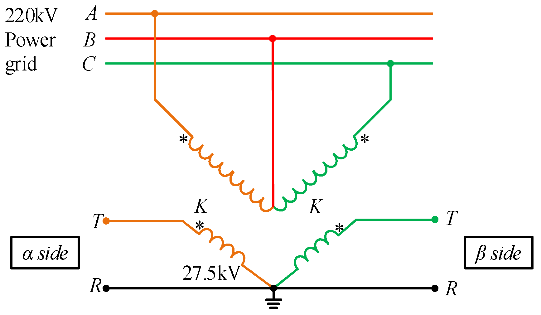
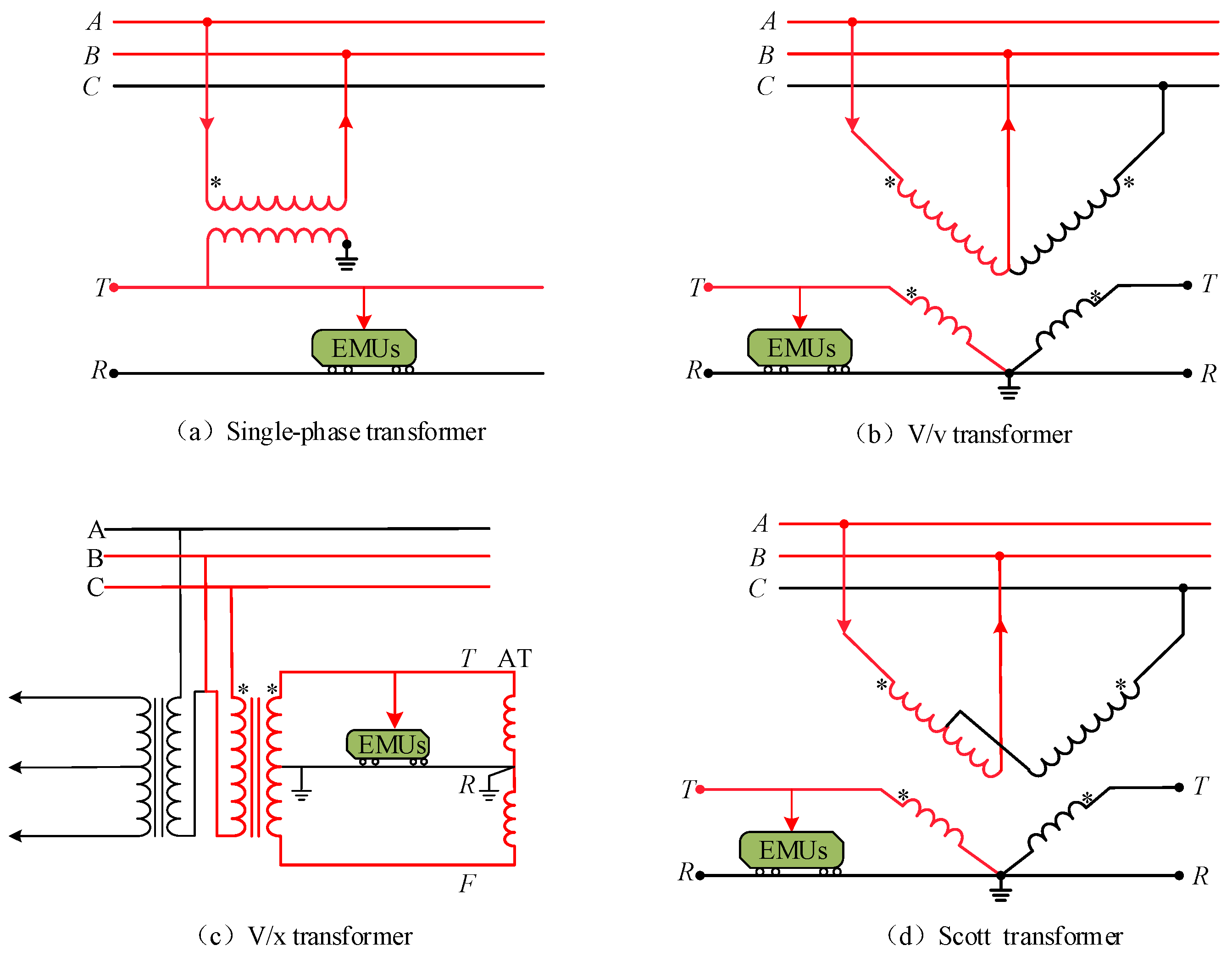
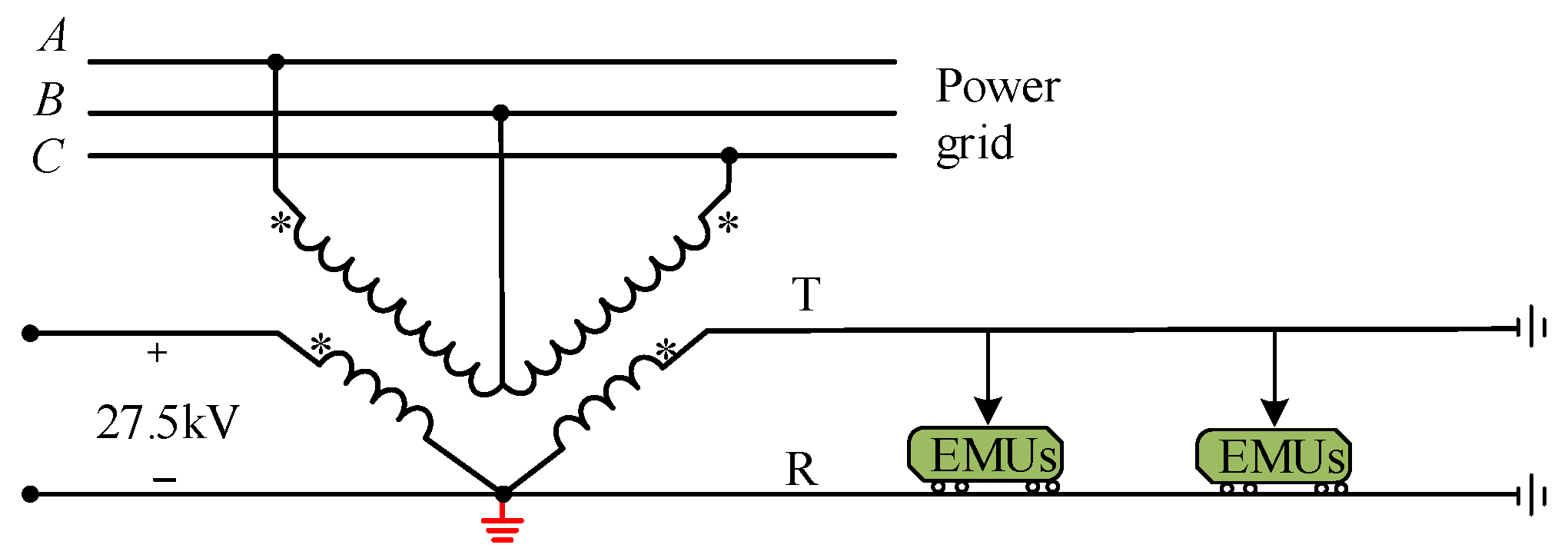
2.2. V/v Traction Transformer Branch Admittance Modeling

The V/v traction transformer is a key component in this modeling process, as illustrated in Figure 5. By formulating the voltage balance equations and magnetomotive force balance equations for the transformer, the nodal admittance equations can be derived, as shown in Equation (1).
The nodal admittance matrix on the alpha side of the V/v transformer is given by
I ˙ A I ˙ B I ˙ C I ˙ T I ˙ R I ˙ F = y T 1 1 0 k k 0 1 1 0 k k 0 0 0 0 0 0 0 k k 0 k 2 k 2 0 k k 0 k 2 k 2 0 0 0 0 0 0 0 U ˙ A U ˙ B U ˙ C U ˙ T U ˙ R U ˙ F
where
y T = y 1 y 2 k 2 y 1 + 2 y 2
In these equations, k represents the transformer turns ratio, while y 1 and y 2 denote the equivalent admittances of the high-voltage and low-voltage sides, respectively.

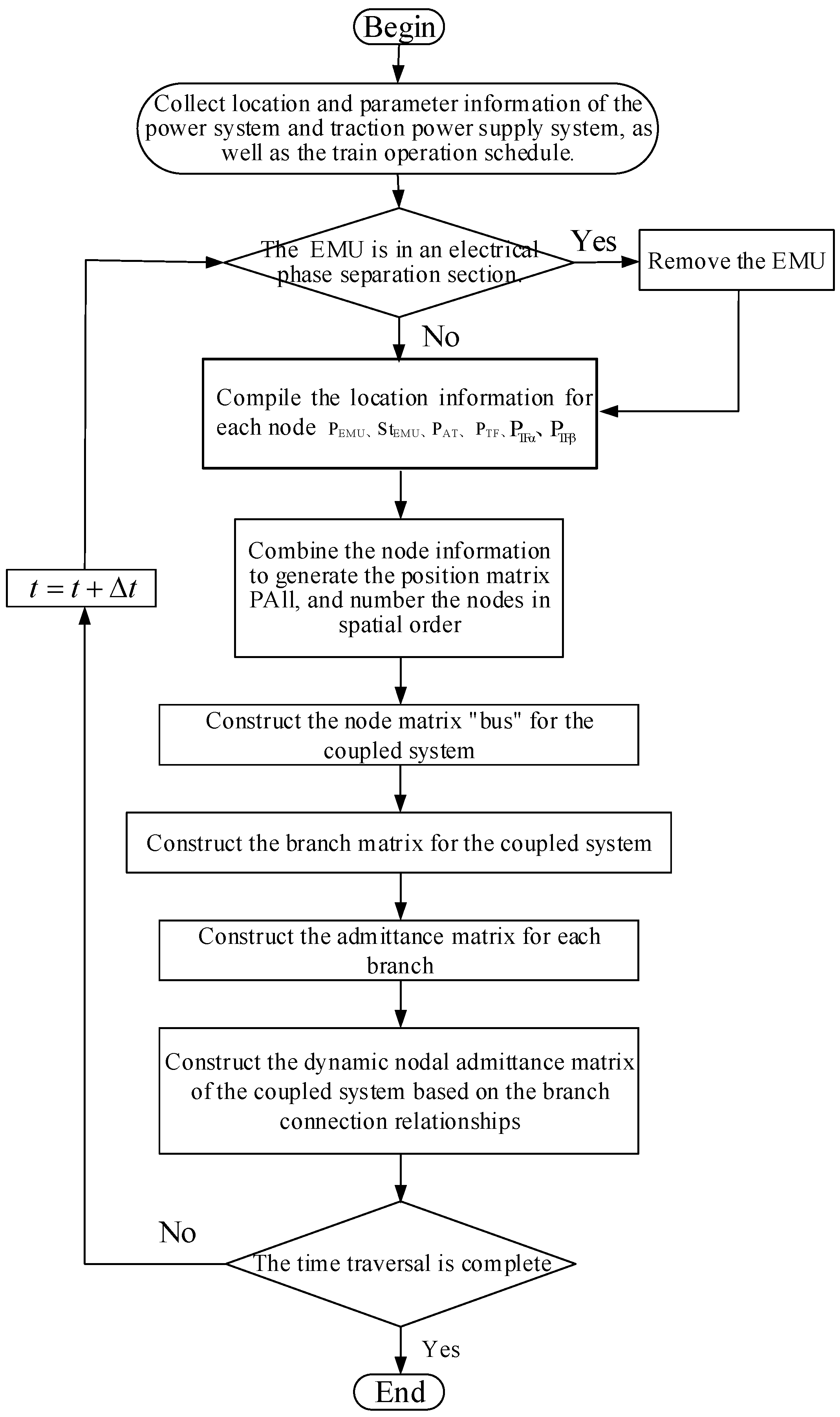
2.3. Construction of Dynamic Nodal Admittance Matrix for Coupled Systems

In the “renewable energy–power grid–transportation network” coupled system, the dynamic changes in the position of EMUs lead to continuous variations in the nodal admittance matrix of the entire system. Below is a method for constructing a dynamic nodal admittance matrix for the coupled system. The process is shown in Figure 6.
Step 1: Based on the train operation schedule, collect position information for each node. Specifically, sequentially represent the EMUs position information using PCRH, for example, PCRH = [5, 15]. The up/down direction of the EMUs is represented by StCRH, where elements in StCRH are either 1 or −1, with 1 indicating the up direction and -1 indicating the down direction. The position information of post stations or shunting points is represented by PAT, such as PAT = [0, 10, 20]. The position information of traction substations is represented by PTF, with the outlet positions of the left and right power supply arms denoted as PTFα and PTFβ, respectively.
Step 2: Determine if an EMUs is located within a neutral section. If it is, remove it; otherwise, proceed to the next step.
Step 3: Combine the node information from Step 1 to generate a position matrix PositionAll, and sort it in ascending order. If there are duplicate elements, remove them directly.
Step 4: Assign node numbers to EMUs, post stations, and traction substations in spatial order.
Step 5: Based on the node numbers from Step 4, and in combination with new energy nodes, generator nodes, and other nodes on the grid side, construct a node matrix (bus) for the coupled system. Each element in the PositionAll matrix constitutes a node, which is set as a load node.
Step 6: Adjacent nodes on the grid side form a branch, and adjacent nodes in the PositionAll matrix also form a branch, thereby constructing a branch connection matrix (branch).
Step 7: For each branch, construct a branch admittance matrix.
Step 8: Construct the nodal admittance matrix based on the branch connection relationships and the EMU up/down matrix StCRH, in conjunction with the branch admittance matrix. Two connection matrices are used: Cf for the branch-to-outgoing-node connection matrix and Ct for the branch-to-incoming-node connection matrix, with dimensions of nl × nb. The elements are defined as follows:
C f ( i , j ) = 1 , j = b r a n c h ( i , f ) C t ( i , k ) = 1 , k = b r a n c h ( i , t )
where i is the branch index, f is the outgoing node of branch i, and t is the incoming node of branch i. nl represents the number of branches, and nb represents the number of nodes.
Therefore, we have the following node voltage connection relationship and node injected current connection relationship:
V f = C f V , V t = C t V I = C f T I f + C t T I t
where I is the total node injected current vector, If is the injected current vector at the outgoing nodes, It is the injected current vector at the incoming nodes, V is the total node voltage vector, Vf is the voltage vector at the outgoing nodes, and Vt is the voltage vector at the incoming nodes.
Based on the branch admittance matrix, we have:
I f = [ Y f f ] V f + [ Y f t ] V t   = [ Y f f ] C f V + [ Y f t ] C t V   = ( [ Y f f ] C f + [ Y f t ] C t ) V I t = ( [ Y t f ] C f + [ Y t t ] C t ) V
where [Y] represents a matrix with elements Y on its diagonal.
Substituting Equation (4) into Equation (5), we obtain
I = C f T ( [ Y f f ] C f + [ Y f t ] C t ) V + C t T ( [ Y t f ] C f + [ Y t t ] C t ) V   = C f T ( [ Y f f ] C f + [ Y f t ] C t ) + C t T ( [ Y t f ] C f + [ Y t t ] C t ) V
Therefore, the nodal admittance matrix of the system is
Y b u s = C f T ( [ Y f f ] C f + [ Y f t ] C t ) + C t T ( [ Y t f ] C f + [ Y t t ] C t )   = C f T [ Y f f ] C f + C f T [ Y f t ] C t + C t T [ Y t f ] C f + C t T [ Y t t ] C t   = C f T Y f f d C f + C f T Y f t d C t + C t T Y t f d C f + C t T Y t t d C t
It should be noted that since the PositionAll matrix varies with time, Ybus also varies with time. Therefore, Ybus is the dynamic nodal admittance matrix of the coupled “renewable energy–power grid–transportation network” system.

3. Dynamic Power Flow Calculation for the Hybrid Asymmetric System of the “Renewable Energy–Power Grid–Transportation Network”

3.1. The Construction of Hybrid Power Flow Equations for the Coupled System of Power Grid and Transportation Network

In regional transmission networks with large-scale traction loads, such as those along mountainous railway lines, the power grid and the traction network naturally form a coupled system, interconnected through traction transformers. Generally, the power system is a three-phase transmission system, while the number of phases in the traction power supply system varies with the traction network’s power supply method. The direct power supply method with a return line is essentially a single-phase transmission system, where the contact wire (T) serves as the transmission phase and the rail (R) acts as the return path, thus formally appearing as a “two-phase transmission”. Additionally, the phases of the contact wires in the left and right supply arms of the traction network are usually different, depending on the type of traction transformer. Therefore, in this coupled system, the three-phase power flow is often unbalanced.
From the perspective of the entire system, when studying the coupled power flow characteristics of both the power grid side and the traction network side simultaneously, it is necessary to consider the power flow equations of the coupled system that encompass both sides. Therefore, it is essential to establish the correspondence between the phase sequences A, B, and C on the power grid side and the phase sequences T, F, and R on the traction side. The principle of phase sequence correspondence is based on the same-name terminals of the transformer windings. Figure 7 illustrates the phase sequence correspondence for a V/v traction transformer.
Therefore, based on the phase sequence correspondence between the power grid side and the traction side, the injection power equation of the coupled system can be written. Taking phase A as an example, the entire equation consists of two parts, as shown in Equations (8) and (9).
P i a = U i a j = 1 N P G m Ω P G ( G i j a m cos θ i a j m + B i j a m sin θ i a j m ) U j m + j = N P G + 1 N m Ω T N ( G i j a m cos θ i a j m + B i j a m sin θ i a j m ) U j m
Q i a = U i a j = 1 N P G m Ω P G ( G i j a m sin θ i a j m B i j a m cos θ i a j m ) U j m + j = N P G + 1 N m Ω T N ( G i j a m sin θ i a j m B i j a m cos θ i a j m ) U j m
G i j x y = g i j x y         j i k = 1 , k i n ( g i k x y + g i k x y o ) = g i i x y + k = 1 , k i n g i k x y j = i x , y Ω P G     o r     Ω T N
B i j x y = b i j x y         j i k = 1 , k i n ( b i k x y + b i k x y o ) = b i i x y + k = 1 , k i n b i k x y j = i x , y Ω P G     o r     Ω T N
where Pia represents the active power injected into phase A at node i, Qia represents the reactive power injected into phase A at node i, NPG denotes the set of nodes on the power grid side, and NTN denotes the set of nodes on the traction network side. ΩPG represents the set of transmission phases on the power grid side, with ΩPG = {a, b, c}. ΩTN represents the set of transmission phases on the traction network side; if the traction network uses direct power supply, then ΩTN = {T, R}.
For convenience, based on the phase sequence correspondence between the power grid side and the traction side, the basic injection power Equations (8) and (9) can be combined into the form shown in Equation (12).
P i a = U i a j = 1 N m Ω ( G i j a m cos θ i a j m + B i j a m sin θ i a j m ) U j m Q i a = U i a j = 1 N m Ω ( G i j a m sin θ i a j m B i j a m cos θ i a j m ) U j m Ω = a , b , c
Therefore, the three-phase injection power equation for any node i can be obtained as shown in Equation (13).
P i a = U i a j = 1 N m Ω ( G i j a m cos θ i a j m + B i j a m sin θ i a j m ) U j m Q i a = U i a j = 1 N m Ω ( G i j a m sin θ i a j m B i j a m cos θ i a j m ) U j m P i b = U i b j = 1 N m Ω ( G i j a m cos θ i a j m + B i j a m sin θ i a j m ) U j m Q i b = U i b j = 1 N m Ω ( G i j a m sin θ i a j m B i j a m cos θ i a j m ) U j m P i c = U i c j = 1 N m Ω ( G i j a m cos θ i a j m + B i j a m sin θ i a j m ) U j m Q i c = U i c j = 1 N m Ω ( G i j a m sin θ i a j m B i j a m cos θ i a j m ) U j m Ω = a , b , c

3.2. A Three-Phase Power Balance Strategy Considering Renewable Energy and Traction Loads

Currently, traction transformers commonly used in traction power supply systems include the single-phase transformer, the V/v transformer, the V/x transformer, and the Scott transformer. The wiring diagrams for each type of traction transformer are shown in Figure 8. It can be seen that for a single EMUs, its power is drawn from two phases of the power grid (either AB, BC, or AC phases). When considering an asymmetric coupled system for a “renewable energy–power grid–transportation network” in mountainous regions, it is necessary to consider the power conversion of the EMUs to the A, B, and C three-phase powers, and thereby establish a three-phase power balance strategy that takes into account renewable energy and traction loads.

3.2.1. The Conversion Relationship Between the Power of the EMUs and the Three-Phase Power at the High-Voltage Side of the Traction Transformer

For convenience, taking the V/v wiring traction transformer as an example (the situation for V/x wiring is consistent with that of V/v wiring), as shown in Figure 9, we will derive the conversion relationship between the power of the EMUs and the three-phase power when the EMUs is on the α side.
Assuming the phase of the A-phase voltage is 0, we have
U ˙ A = U A 0 U ˙ B = U B 120 U ˙ C = U C 120 U A = U B = U C
Assuming the angle of current of the EMUs on the alpha side and the voltage is θ, then we have
U ˙ α = U ˙ A U ˙ B K = 3 U A 30 K I ˙ α = I 30 θ
where I is the amplitude of the EMUs current I · α , and K is the transformer ratio.
Further, we can derive that:
I ˙ A = I 30 θ K I ˙ B = I 30 θ K
Therefore, the apparent power of the EMUs on the alpha side can be represented as:
S ˙ α = U ˙ α I ˙ α = 3 U A 30 K I θ 30   = 3 U A I cos θ K + j 3 U A I sin θ K   = P C R H + j Q C R H
where PCRH and QCRH represent the active power and reactive power of the EMUs on the alpha side, respectively.
The apparent power of phase A on the high-voltage side of the traction transformer is
S ˙ A = U ˙ A I ˙ A = U A K I θ 30   = U A I K cos θ 30 + j U A I K sin θ 30   = U A I K 3 2 cos θ + 1 2 sin θ + j U A I K 3 2 sin θ 1 2 cos θ   = P A + j Q A
By substituting Equation (17) into Equation (18), we can obtain the conversion relationship between the power of phase A on the high-voltage side of the traction transformer and the power of the EMUs, as shown in Equation (19)
P A = P C R H 2 + Q C R H 2 3 Q A = Q C R H 2 P C R H 2 3
The apparent power of phase B on the high-voltage side of the traction transformer is
S ˙ B = U ˙ B I ˙ B = U A 120 I ˙ A   = U A I K θ 150   = U A I K cos θ 150 j U A I K sin θ 150   = U A I K 3 2 cos θ 1 2 sin θ + j U A I K 3 2 sin θ + 1 2 cos θ   = P B + j Q B
By substituting Equation (17) into Equation (20), we can obtain the conversion relationship between the power of phase B on the high-voltage side of the traction transformer and the power of the EMUs, as shown in Equation (21).
P B = P C R H 2 Q C R H 2 3 Q B = Q C R H 2 + P C R H 2 3
Similarly, when the EMUs are on the β side, the conversion relationship between the power of phases B and C on the high-voltage side of the traction transformer and the power of the EMUs is given by Equation (22).
P B = P C R H 2 + Q C R H 2 3 Q B = Q C R H 2 P C R H 2 3 P C = P C R H 2 Q C R H 2 3 Q C = Q C R H 2 + P C R H 2 3

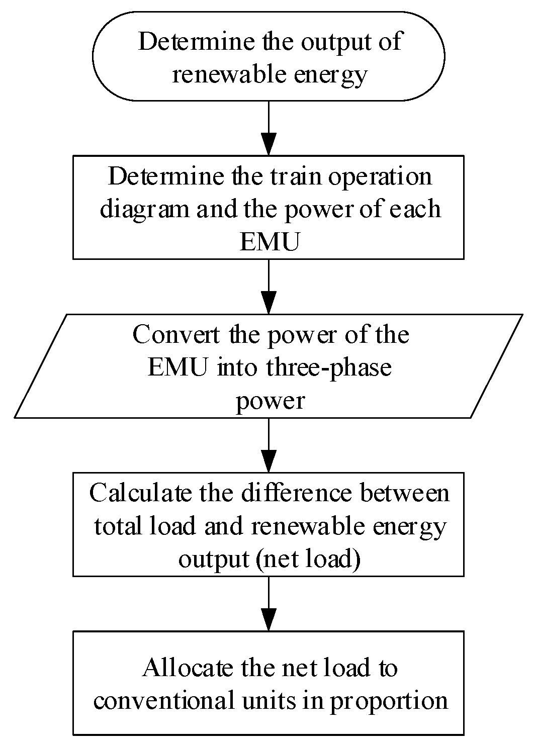
3.2.2. The Strategy Process for Power Balance Considering Renewable Energy and Traction Load

Due to the inclusion of renewable energy nodes in the system, in order to achieve the goals of energy conservation and emission reduction, priority is given to utilizing renewable energy output to supply power to loads during power flow calculations. Therefore, the strategy process for power balance considering renewable energy and traction load is shown in Figure 10. The specific steps are as follows:
Step 1: Determine the renewable energy output at each node.
Step 2: Determine the train operation schedule and obtain the power of each EMUs based on traction calculations.
Step 3: Convert the power of each EMUs into three-phase power based on the wiring configuration of the traction transformer.
Step 4: Calculate the difference between the total load and the renewable energy output, which is referred to as the net load.
Step 5: Allocate the net load to each conventional power generation unit based on their installed capacity ratio.

3.3. Solving the Nonlinear Equations for Hybrid Power Flow in a Coupled System

3.3.1. Matrix Partitioning

After processing various types of nodes, the hybrid power flow calculation equations for the coupled system can be formed. Suppose there is one slack node, m PV nodes, n1 grid-side PQ nodes, and n2 traction-side PQ nodes (where n1 + n2 = n) in the entire system network. Additionally, (m + 1) generator internal potential nodes are added, resulting in a total of (n + 2m + 2) nodes in the system. Let R represent the slack node and W represent the internal potential node of the slack node. Let S denote the set of PV nodes, S = {s1, s2, …, sm}. Let Z denote the set of all internal potential nodes for PV nodes, Z = {z1, z2, …, zm}. Let L represent the set of grid-side PQ nodes, L = {l1, l2, …, ln1}. Let Γ represent the set of traction-side PQ nodes, Γ = {γ1, γ2, …, γn2}. Define the following:
P R = P R a P R b P R c T , Q R = Q R a Q R b Q R c T P W = P W a P W b P W c T , Q W = Q W a Q W b Q W c T P S = P s 1 a P s 1 b P s 1 c P s m a P s m b P s m c T Q S = Q s 1 a Q s 1 b Q s 1 c Q s m a Q s m b Q s m c T P Z = P z 1 a P z 1 b P z 1 c P z m a P z m b P z m c T Q Z = Q z 1 a Q z 1 b Q z 1 c Q z m a Q z m b Q z m c T P L = P l 1 a P l 1 b P l 1 c P l n 1 a P l n 1 b P l n 1 c T Q L = Q l 1 a Q l 1 b Q l 1 c Q l n 1 a Q l n 1 b Q l n 1 c T P Γ = P γ 1 a P γ 1 b P γ 1 c P γ n 2 a P γ n 2 b P γ n 2 c T Q Γ = Q γ 1 a Q γ 1 b Q γ 1 c Q γ n 2 a Q γ n 2 b Q γ n 2 c T
In the equations, PR represents the three-phase active power matrix of the slack node and QR represents the three-phase reactive power matrix of the slack node. PW denotes the three-phase active power matrix of the internal potential node of the slack node, and QW denotes the three-phase reactive power matrix of the internal potential node of the slack node. PS represents the three-phase active power matrix of the PV nodes, and QS represents the three-phase reactive power matrix of the PV nodes. PZ denotes the three-phase active power matrix of the internal potential nodes of the PV nodes, and QZ denotes the three-phase reactive power matrix of the internal potential nodes of the PV nodes. PL represents the three-phase active power matrix of the grid-side PQ nodes, and QL represents the three-phase reactive power matrix of the grid-side PQ nodes. PΓ denotes the three-phase active power matrix of the traction-side PQ nodes, and QΓ denotes the three-phase reactive power matrix of the traction-side PQ nodes.
The voltage magnitude and phase are partitioned in the same block manner as shown in the equation.
U X = U R X T U W X T U S X T U Z X T U L X T U Γ X T T , X = A , B , C θ X = θ R X T θ W X T θ S X T θ Z X T θ L X T θ Γ X T T , X = A , B , C
where UA, UB, and UC represent the three-phase voltage magnitude matrices, while θA, θB, and θC represent the three-phase angle matrices, respectively.

3.3.2. Handling of Boundary Conditions for the Traction Power Supply System

For a direct power supply system, since there is no positive feeder line F, only two phases exist on the traction side. Therefore, we can assume that the voltage of the virtual positive feeder line is zero and does not participate in the iterative solution process of the equations, i.e.,
U ˙ Γ F = 0  
In addition, the neutral point on the secondary side of the traction transformer needs to be grounded. Therefore, the voltage at this point is zero and does not participate in the iterative solution process of the equations, as show in Figure 11.
Therefore, in light of the aforementioned boundary conditions, it is necessary to eliminate the variables from Equation (24) that do not participate in the iterative solution. Let U Γ X and θ Γ X denote the voltage magnitude matrix and phase angle matrix, respectively, after eliminating the variables on the traction side that do not participate in the iterative solution.

3.3.3. Handling of Boundary Conditions on the Power Grid Side

For generator nodes, remove the reactive power and voltage magnitude of PV nodes, and remove the voltage magnitude and phase angle of the slack node.
Combining Equations (23)–(25), and partitioning the admittance matrix, we can obtain the power flow iteration equation, as shown in Equation (26).
Δ P p Δ Q p = F p H p H p F p Δ θ p Δ U p = J T Δ θ p Δ U p
The Newton–Raphson iteration method is used for the solution. From the equation, the corrections Δ θ p ( k + 1 ) and Δ U p ( k + 1 ) for the (k + 1)th iteration can be obtained, thereby yielding a new solution.
θ p ( k + 1 ) U p ( k + 1 ) = θ p ( k ) U p ( k ) Δ θ p ( k + 1 ) Δ U p ( k + 1 )
This iterative calculation process is repeated until convergence is achieved for all nodes’ Δ θ < ε and Δ U < ε .

4. Case Study Analysis

A regional “renewable energy–power grid–transportation network” in China is used as a case study to analyze and verify the proposed method for power flow calculations in coupled systems. The topological structure at a specific moment is illustrated in Figure 12, which comprises 18 traction stations (all equipped with V/v connected transformers), 15 conventional hydropower units, and 2 new energy stations, with a total railway length of 663 km. The three-phase node scale is approximately 1000 nodes, which may vary depending on the operational schedule. The local load is set at 1000 MW, while the traction load is about 300 MW.
Based on the operational schedule shown in Figure 13, the conditions for high-speed train operations are established, with power flow calculations performed every 2 s to record the node voltage magnitudes and phase angles.

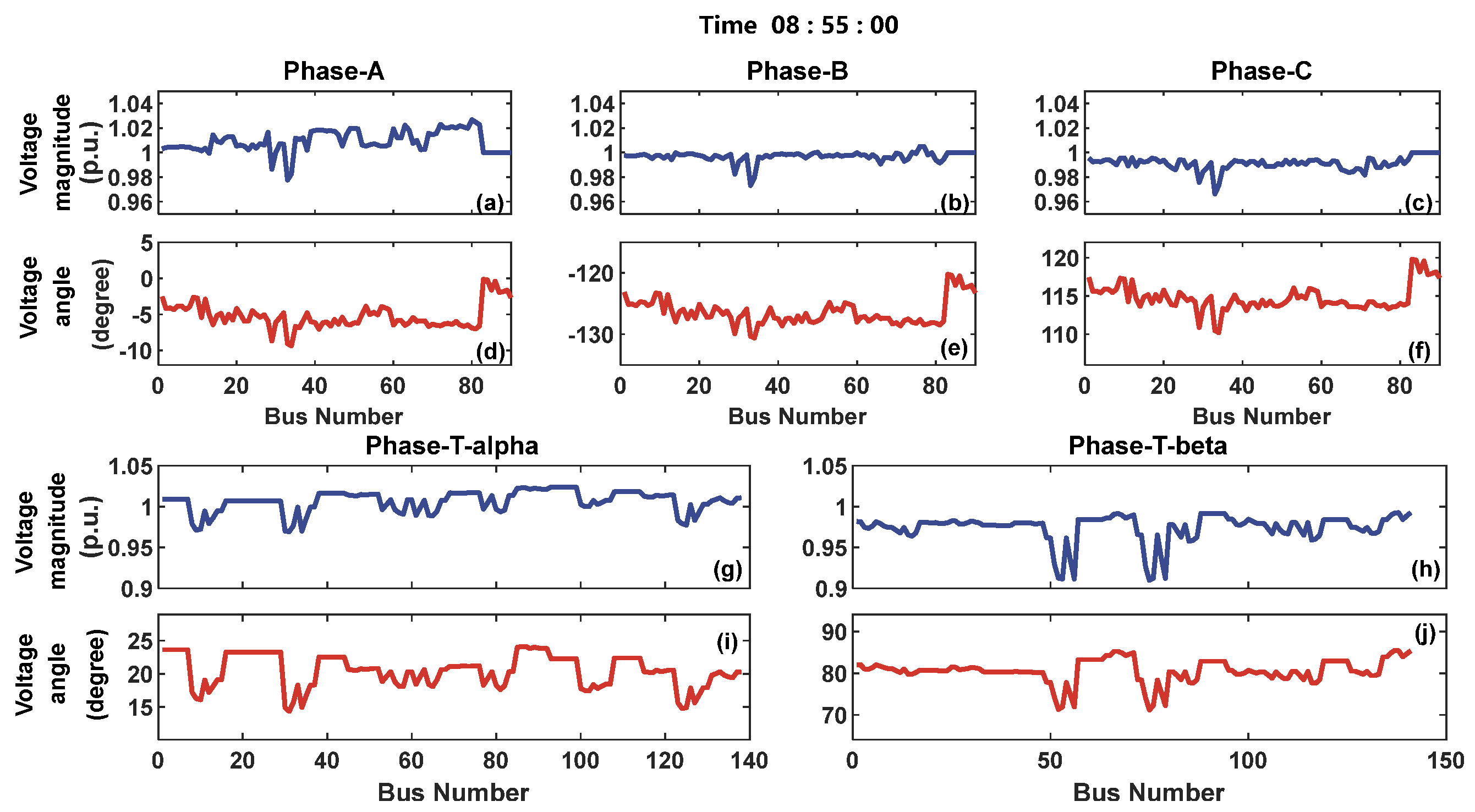
4.1. Analysis of Multi-Vehicle Single-Time Section Results

The computational results at 08:55:00 are presented in Figure 14, where subfigures (a) to (f) depict the three-phase node voltages and phase angles on the grid side, encompassing a total of 101 three-phase nodes. Subfigures (g) to (j) represent the voltage and phase angles at the traction side contact line nodes, including nodes on the alpha side (138 nodes) and the beta side (141 nodes). It is important to note that the horizontal axis in the figure does not represent node numbering but rather the number of nodes.
It can be observed that the voltage phase angles for phases A, B, and C are sequentially separated by 120°, with voltage magnitudes stabilizing around the per unit value of 1. Table 1 lists the average phase angles for the three phases on the grid side and the alpha and beta sides of the traction supply. The average phase angle for the traction alpha side is 20.44°, while the average phase angle for phase A on the grid side is −4.9439°, resulting in a difference of 25.3839°. Additionally, the average phase angle for the traction beta side is 80.5516°, compared to an average phase angle of 115.0173° for phase C on the grid side, which results in a difference of 34.4657°. This discrepancy is determined by the structure of the V/v transformer.

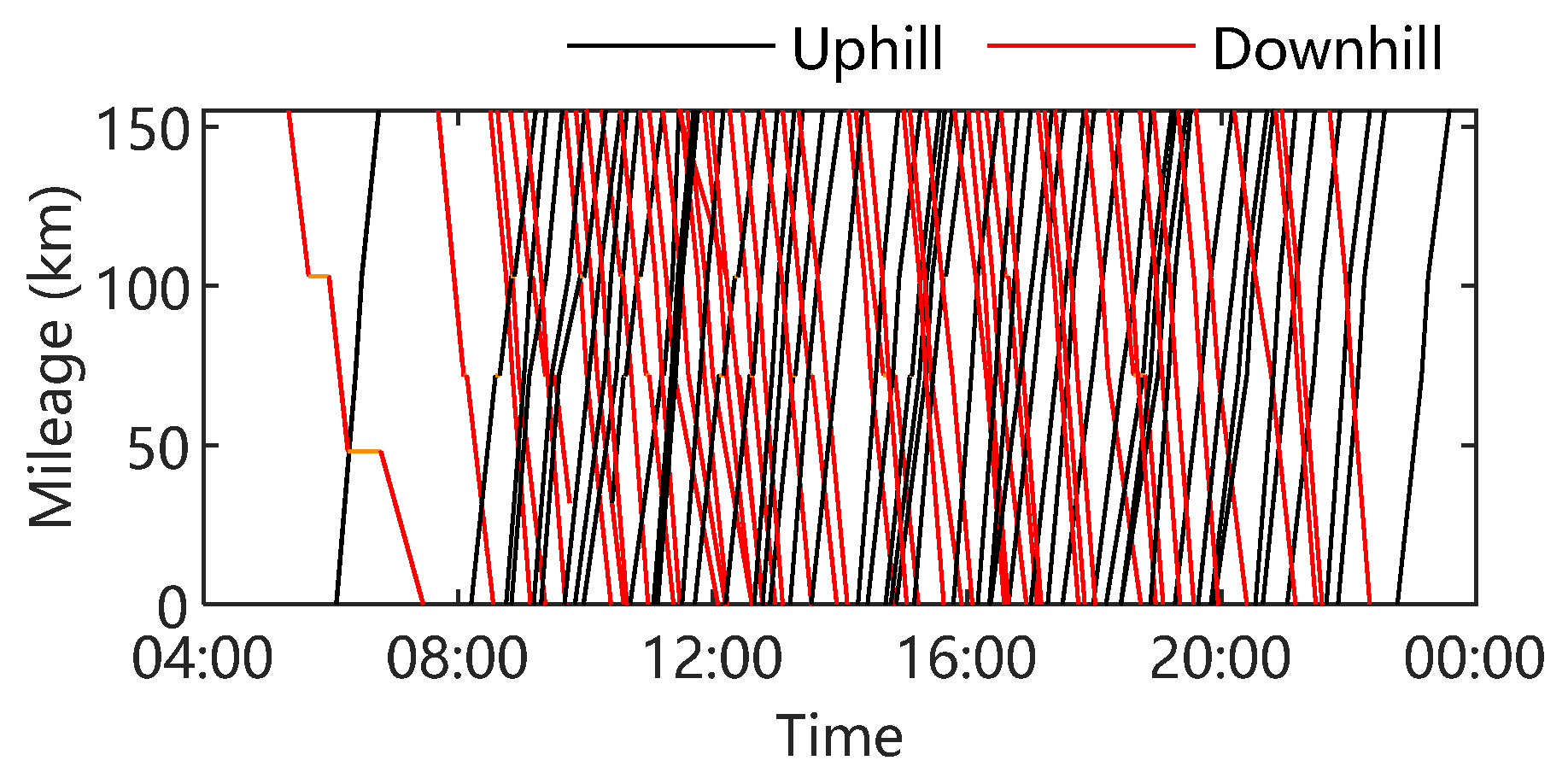
4.2. Analysis of Continuous Operation Conditions for Single Vehicles

Figure 15a illustrates the operational conditions of the last vehicle as it moves through the supply ranges of Traction Substation 2 and Traction Substation 3. The locomotive begins its ascent on an incline with a gradient of 30‰ and subsequently descends a slope with a gradient of 13.7‰ after passing through Traction Substation 2, encountering three-phase separation points during the process. Figure 15b illustrates the variation in the active power of the locomotive. During the uphill phase, the locomotive power is approximately 18.2 MW. In the downhill phase, the locomotive operates in regenerative braking mode, with a return power of approximately −4.8 MW. The power is considered to be zero during the neutral section passing.
Figure 15c,d show the variations in the pantograph voltage and phase of the EMUs, with the three-phase separation points dividing the curve into four segments. The first segment corresponds to the ascent, while the second to fourth segments pertain to the descent. A comparative analysis between the uphill traction condition (Figure 15e) and downhill braking conditions (Figure 15f–h) reveals that the pantograph voltage during braking operation is significantly higher than during traction, attributable to the locomotive’s regenerative power feedback. This phenomenon demonstrates the distinctive voltage elevation effect inherent in traction power supply systems.
Moreover, as indicated in Figure 15i–l, there are noticeable jumps in the phase of the pantograph voltage at both sides of each phase transition. One side approaches 30°, while the other side approaches 90°. This phenomenon is attributed to the different phase sequences of the power supply arms from the grid on either side of the phase transition, illustrating the dynamic characteristics of the high-speed train during operation.

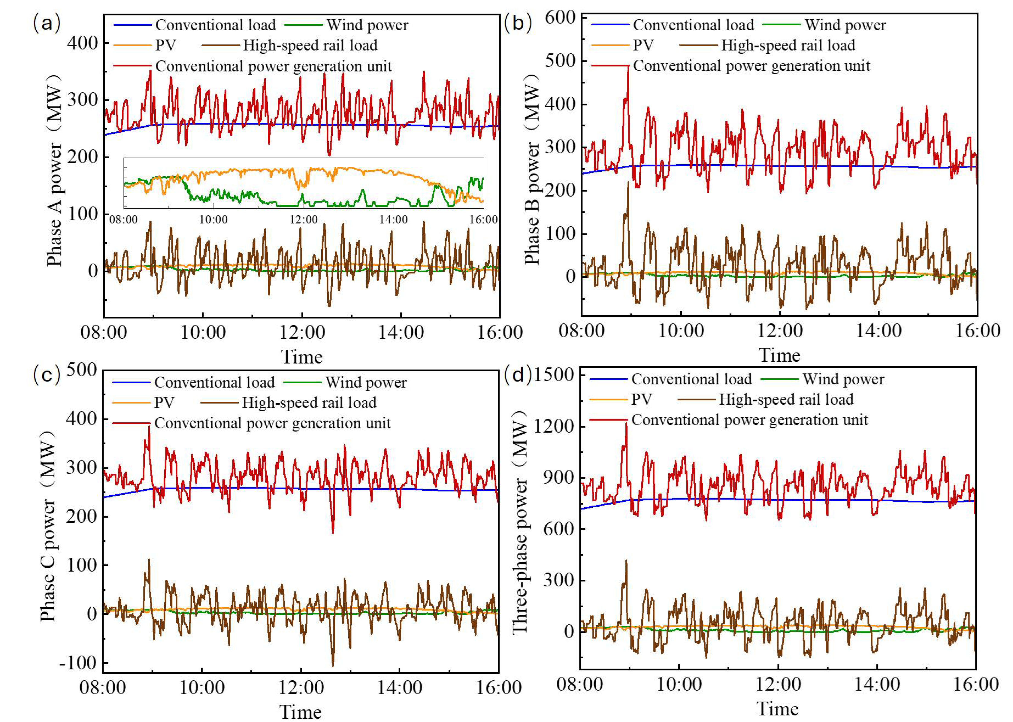
4.3. Analysis of System Operation Results

The system operation results at the time interval of 8:00 to 16:00 are illustrated in Figure 16. In the figure, subfigures (a) to (c) represent the power levels for phases A, B, and C, respectively, while subfigure (d) depicts the total three-phase power of the system. From the observations, it is evident that the influence of long steep grades leads to significant traction power demands and substantial, frequent regenerative braking power from the EMUs. This results in increased fluctuations in high-speed railway loads. During these pronounced fluctuations, conventional units also adjust to follow the variations, indicating that the three-phase power balance strategy proposed in this study, which takes into account renewable energy and traction loads, is effective in regulating the power of asymmetric coupling systems in mountainous regions.
Since the three-phase output from wind and photovoltaic sources is balanced, this analysis focuses on phase A. As shown in subfigure (a), although the output from wind and photovoltaic sources experience considerable fluctuations, the two sources exhibit good complementary characteristics. This complementary behavior mitigates the impact of these fluctuations on the overall system.
While the proposed dynamic power flow framework advances the analysis of renewable energy–power grid–transportation network coupled systems, two key limitations warrant attention.
Hybrid Asymmetric System Complexity: The algorithm requires the specialized handling of missing-phase dynamics in single-phase traction networks interfaced with three-phase grids. Future work could integrate phase-balancing techniques or adaptive machine learning models to simplify unbalanced condition resolution.
Computational Overhead: Dynamic admittance matrix updates and high-dimensional nonlinear equations impose significant computational costs. Although parallel computing offers partial mitigation, real-time deployment necessitates further optimizations, such as precomputed admittance templates or sparse solver integration. Addressing these challenges will enhance the framework’s scalability for large-scale, real-time applications.

5. Conclusions

This paper presents a dynamic power flow calculation method for a “renewable energy–power grid–transportation network” asymmetric coupling system. By utilizing the asymmetric characteristics of traction transformers, we establish a dynamic asymmetric nodal admittance matrix for the coupling system. This, in turn, allows us to develop a mixed power flow equation for the coupling system and propose a three-phase power balance strategy that considers renewable energy and traction loads. This strategy addresses the challenge of converting single-phase powers on the traction side to three-phase powers (A, B, C) on the grid side. Finally, simulations are conducted using a practical example of a regional power grid–traction network system, leading to the following conclusions:
  • In light of the severe fluctuations of high-speed railway loads in mountainous regions, the three-phase power balance strategy proposed in this study, which considers both renewable energy and traction loads, effectively regulates the power in such asymmetric coupling systems.
  • Due to the structural influence of the traction transformer, there is a significant difference in the average phase values between the three phases on the grid side and the alpha and beta phases on the traction side.
  • Under braking conditions, the pantograph voltage is significantly higher than that in traction mode compared to the regenerative power feedback from the locomotive, which manifests a distinct voltage elevation effect in the traction power supply system. At both sides of each neutral section, the phase angle exhibits jumps influenced by the different phase-sequence power supply from the grid.

Author Contributions

Conceptualization, B.L.; Methodology, Q.Z.; Investigation, J.L., Y.S. and Z.L.; Visualization, Q.Z.; Data curation, D.Z. All authors have read and agreed to the published version of the manuscript.

Funding

This work was supported by Science and Technology Project of State Grid Sichuan Electric Power Company (research on the joint planning method of hybrid asymmetrical system of a “renewable energy–power grid–transportation network” in high-altitude areas adapted to new energy access) (ERP: 52199624000B).

Conflicts of Interest

Author Bo Li was employed by State Grid Sichuan Electric Power Company. The remaining authors declare that the research was conducted in the absence of any commercial or financial relationships that could be construed as a potential conflict of interest.

References

  1. Trias, A. The Holomorphic Embedding Load Flow method. In Proceedings of the 2012 IEEE Power and Energy Society General Meeting, San Diego, CA, USA, 22–26 July 2012; pp. 1–8. [Google Scholar]
  2. Subramanian, M.K.; Feng, Y.; Tylavsky, D. PV bus modeling in a holomorphically embedded power-flow formulation. In Proceedings of the 2013 North American Power Symposium (NAPS), Manhattan, KS, USA, 22–24 September 2013; pp. 1–6. [Google Scholar]
  3. Rao, S.; Feng, Y.; Tylavsky, D.J.; Subramanian, M.K. The Holomorphic Embedding Method Applied to the Power-Flow Problem. IEEE Trans. Power Syst. 2016, 31, 3816–3828. [Google Scholar] [CrossRef]
  4. Chiang, H.D.; Wang, T.; Sheng, H. A Novel Fast and Flexible Holomorphic Embedding Power Flow Method. IEEE Trans. Power Syst. 2018, 33, 2551–2562. [Google Scholar] [CrossRef]
  5. Goodman, C.J.; Kulworawanichpong, T. Sequential linear power flow solution for AC electric railway power supply systems. WIT Trans. Built Environ. 2002, 61, 10. [Google Scholar]
  6. Goodman, C.J.; Kulworawanichpong, T. Sequential Linear Power Flow Solution for AC Electric Railway Power Supply Systems; WIT Press: Southampton, UK, 2002; pp. 531–540. [Google Scholar]
  7. Zhang, W.; Yang, S.; Zhang, J.; Ye, J.; Wu, M. A two-phase power flow algorithm of traction power supply system based on traction substation-network decoupling. Int. J. Electr. Power Energy Syst. 2023, 152, 109252. [Google Scholar] [CrossRef]
  8. He, J.W.; Li, Q.Z.; Liu, W.; Zhou, X.H. General mathematical model for simulation of AC traction power supply system and its application. Power Syst. Technol. 2010, 34, 25–29. [Google Scholar]
  9. Hongwei, C.; Guangchao, G.; Quanyuan, J. Power flow algorithm for traction power supply system of electric railway based on locomotive and network coupling. Autom. Electr. Power Syst. 2012, 36, 76–80+110. [Google Scholar]
  10. Fang, W.; Xiaoru, W. A power flow analysis method of traction power supply system based on constant-power load. Proc. CSU-EPSA 2015, 27, 59–64. [Google Scholar]
  11. Wan, Q.; Wu, M.; Chen, J.; Wang, Z.; Liu, X. Simulating calculation of traction substation’s feeder current based on traction calculation. Trans. China Electrotech. Soc. 2007, 22, 108–113. [Google Scholar]
  12. Xiaoqin, L.; Xiaoru, W. State-space model of high-speed railway traction power-supply system. Proc. CSEE 2017, 37, 857–868. [Google Scholar]
  13. Junqi, Z.; Mingli, W. Power flow algorithm for electric railway traction network based on multiple load port equivalence. Trans. China Electrotech. Soc. 2018, 33, 2479–2485. [Google Scholar]
  14. Mongkoldee, K.; Kulworawanichpong, T. Current-based Newton-Raphson power flow calculation for AT-fed railway power supply systems. Int. J. Electr. Power Energy Syst. 2018, 98, 11–22. [Google Scholar]
  15. Hui, W.; Wei, L.; Qunzhan, L.; Qing, M.; Tongtong, L. Dynamic power flow calculation of AC electrified railway based on unified chain circuit of source-network-load. J. China Electrotech. Soc. 2022, 42, 3936–3953. [Google Scholar]
  16. Hu, H.; He, Z.; Li, X.; Wang, K.; Gao, S. Power-Quality Impact Assessment for High-Speed Railway Associated with High-Speed Trains Using Train Timetable-Part I: Methodology and Modeling. IEEE Trans. Power Deliv. 2016, 31, 693–703. [Google Scholar] [CrossRef]
  17. Hu, H.; He, Z.; Wang, K.; Ma, X.; Gao, S. Power-Quality Impact Assessment for High-Speed Railway Associated with High-Speed Trains Using Train Timetable—Part II: Verifications, Estimations and Applications. IEEE Trans. Power Deliv. 2016, 31, 1482–1492. [Google Scholar] [CrossRef]
  18. Hu, H.; He, Z.; Wang, J.; Gao, S.; Qian, Q. Power Flow Calculation of High-speed Railway Traction Network Based on Train-network Coupling Systems. Proc. CSEE 2012, 32, 101–108. [Google Scholar]
  19. He, Z.; Hu, H.; Zhang, Y.; Gao, S. Harmonic Resonance Assessment to Traction Power-Supply System Considering Train Model in China High-Speed Railway. IEEE Trans. Power Deliv. 2014, 29, 1735–1743. [Google Scholar] [CrossRef]
  20. Mohamed, B.; Arboleya, P.; El-Sayed, I.; González-Morán, C. High-speed 2 × 25 kV traction system model and solver for extensive network simulations. IEEE Trans. Power Syst. 2019, 34, 3837–3847. [Google Scholar] [CrossRef]
Figure 1. Schematic diagram of the coupled system of “renewable energy–power grid–transportation network”.
Energies 18 01567 g001
Figure 2. Schematic diagram of node division for the traction power supply system.
Energies 18 01567 g002
Figure 3. The chain-type circuit structure of the traction network.
Energies 18 01567 g003
Figure 4. Schematic diagram of the coupled system’s topology at times t1 and t2.
Energies 18 01567 g004
Figure 5. Connection diagram of V/v wiring transformer under three-phase ABC incoming line configuration.
Energies 18 01567 g005
Figure 6. The construction process of the dynamic nodal admittance matrix for the coupled system.
Energies 18 01567 g006
Figure 7. The phase sequence correspondence between the traction side and the power grid side of a V/v traction transformer.
Energies 18 01567 g007
Figure 8. Summary of common traction transformer types.
Energies 18 01567 g008
Figure 9. The schematic diagram of the V/v connected traction transformer structure.
Energies 18 01567 g009
Figure 10. Consider a power balancing strategy for renewable energy and traction load.
Energies 18 01567 g010
Figure 11. Schematic diagram of the grounding structure of the direct power supply system.
Energies 18 01567 g011
Figure 12. Schematic diagram of the regional “renewable energy–power grid–transportation network”.
Energies 18 01567 g012
Figure 13. Train operation diagram (partial).
Energies 18 01567 g013
Figure 14. Calculation results at 08:55:00.
Energies 18 01567 g014
Figure 15. Simulation results analysis of single-unit locomotive.
Energies 18 01567 g015
Figure 16. System operation results analysis chart.
Energies 18 01567 g016
Table 1. Average voltage phase angles.
PhasesABC
Average Phase Angle (°)−4.9439−126.095115.0173
Phasesalphabeta
Average Phase Angle (°) 20.4480.5516
Disclaimer/Publisher’s Note: The statements, opinions and data contained in all publications are solely those of the individual author(s) and contributor(s) and not of MDPI and/or the editor(s). MDPI and/or the editor(s) disclaim responsibility for any injury to people or property resulting from any ideas, methods, instructions or products referred to in the content.

