Exploration of Training Strategies for a Quantile Regression Deep Neural Network for the Prediction of the Rate of Penetration in a Multi-Lateral Well

Abstract

In recent years, rate of penetration (ROP) prediction using machine learning has attracted considerable interest. However, few studies have addressed ROP prediction uncertainty and its relation to training data and model inputs. This paper presents the application of a quantile regression deep neural network (QRDNN) for ROP prediction on multi-lateral wells drilled in the Alvheim field of the North Sea. The quantile regression framework allows the characterization of the prediction uncertainty, which can inform the end-user on whether the model predictions are reliable. Three different training strategies for the QRDNN model are investigated. The first strategy uses individual hole sections of the multi-lateral well to train the model, which is then tested on sections of similar hole size. In the second strategy, the models are trained for specific formations encountered in the well, assuming the formation tops are known for both the training and test sections. The third strategy uses training data from offset wells from the same field as the multi-lateral well, exploring different offset–well combinations and input features. The resulting QRDNN models are tested on several complete well sections excluded from the training data, each several kilometers long. The second and third strategies give the lowest mean absolute percentage errors of their median predictions of 27.3% and 28.7% respectively—all without recalibration for the unknown test well sections. Furthermore, the third model based on offset training gives a robust prediction of uncertainty with over 99.6% of actual values within the predicted P10 and P90 percentiles.

1. Introduction

The cost of drilling wells for the exploration of hydrocarbon resources can vary between 30% and 60% of the average well costs [1], while for deep geothermal wells, it can constitute as much as 50% to 75% of the average cost per well [2]. In order to achieve significant cost reduction, it is necessary to reduce the effective drilling time and also the non-productive time associated with the mitigation of drilling incidents such as stuck pipe, loss of drilling fluid to the formation, drill-string twist-off, or equipment failure. The proper selection of drilling parameters, such as the drill-string revolutions per minute (RPM), weight on bit (WOB), and mud pump circulation rate can improve the rate of penetration (ROP) and also prevent the occurrence of drilling incidents, thus reducing both the effective drilling time and the non-productive time. To address this problem, advanced technical solutions for drilling parameter optimization [3] and autonomous decision-making while drilling [4] have been developed in recent years, and a successful demonstration of these technologies has been conducted on a full-scale test rig [5].

A key prerequisite to facilitate optimal drilling parameter selection is the availability of predictive models that can evaluate the ROP in response to different drilling parameter combinations. Earlier ROP models were based on empirical correlations among drilling parameters, with the most notable ones being the Maurer model [6], the Bingham model [7] and the Bourgoyne and Young model [8]. More recent efforts in this direction have been focused on including detailed descriptions of the physics of the cutting process [9] and drill bit wear mechanisms [10]. Physics-based ROP models, such as the ones mentioned earlier, require frequent re-calibration as the downhole conditions (e.g., rock strength, bit wear, or drill-string vibrations) change during drilling [11].

In the past decade, data-driven modeling and machine learning (ML), in particular, have become an attractive alternative to the physics-based modeling of drilling processes, with ROP prediction among its top applications in this area. Artificial intelligence techniques, including ML, have joined model-based approaches across various subsurface-energy-extraction applications [12,13]. A comprehensive literature review by Barbosa et al. [14] indicated that ML-based models can outperform traditional physics-based models in terms of ROP prediction accuracy and flexibility. Sabah et al. [15] compared data mining methods with several machine learning algorithms to evaluate their accuracy and effectiveness in predicting ROP. Khosravanian and Aadnøy [16] provide a recent comprehensive overview of different ML methods for ROP prediction, including artificial neural networks (ANNs), support vector machines, fuzzy inference systems, neurofuzzy models, and ensemble techniques. They emphasize the importance of data-driven modeling in optimizing drilling operations and achieving high ROP. Other commonly used ML algorithms for ROP modeling include random forests [17,18,19,20,21], support vector regression [22,23,24], gradient boosting [20,21,25], the K-Nearest-Neighbors algorithm [26] and recurrent neural networks [18,27,28]. Hybrid methods combining physics with ML are also starting to emerge [29,30], and physics-informed ANNs are starting to emerge in a wider context [31,32], but they are beyond the scope of the current study.

The most frequently used input features for ML-based ROP models are WOB, RPM, hole depth, mud pump rate, mud weight, bit diameter, rock strength and bit wear [14], while some models include more complex features such as bit hydraulics and cuttings transport [33]. Some ML-based ROP models have been deployed into ROP optimization workflows and advisory systems, with reported ROP improvements of up to 33% in field tests [25,34,35].

Despite these positive results, ML-based ROP-prediction models face several practical challenges that might hinder their robustness and acceptance in drilling automation and optimization workflows.

Firstly, when choosing training and test data sets for ROP models, one needs to take into account that drilling data are sequential, and therefore using a random train/test split may lead to models that perform well on the training and test sets but quite poorly when applied to other data sets [36].

Secondly, ROP modeling is affected by the data distribution shift, where the same values of the input variables may produce different ROP values in two different rock formations. To avoid this pitfall, [33] proposed training separate ANN models for individual formations, while [19] applied the same concept for random forest and ensemble ROP models. The results of both studies indicated lower prediction errors for the formation-specific models than models relying on training data from multiple formations, although it can be argued that models trained on a specific formation are more prone to overfitting to that formation. When formation data are hard to estimate, the use of transfer learning that uses part of the data from the well being drilled [37] or a continual learning framework [38] can improve the results.

Finally, DNN models are complex function approximators that are hard for the end user to interpret. One way to improve the interpretability of an ML model is by including a measure of confidence, or rather uncertainty, in its predictions. This information can be critical when the model is used in an advisory system or a fully automated system, such that the user can build trust in the recommendations or actions taken by the system. Only a few studies have addressed uncertainty in ROP prediction, whether for physics-based or ML-based models [14]. Uncertainty can be divided into aleatoric and epistemic [39]. Aleatoric uncertainty arises from the inherent variability in the data, and the output variable (in this case, ROP) is treated as a probability distribution when training the ML model. The epistemic uncertainty results from the choice of model and input features. Ambrus et al. [40] developed an ROP prediction model using a DNN with quantile regression to estimate the aleatoric uncertainty in the prediction. Bizhani and Kuru [39] accounted for both types of uncertainty using a Bayesian neural network for ROP prediction. Both approaches showed promising results on several publicly available drilling data sets.

Verification with practical data is needed to understand how training data selection, input features (including formation data), and uncertainty estimation techniques impact the robustness of ROP prediction. Additionally, it is essential to determine whether the estimated uncertainty can indicate when a trained model is not valid for a test section, even if the mean prediction error remains within acceptable limits.

In this work, we build on the quantile regression DNN (QRDNN) framework to address the aforementioned questions with an application in a multi-lateral well drilled in the Alvheim field in the North Sea and nearby offset wells. The main contribution of this work is the investigation of how the choice of data for training this QRDNN model can affect the prediction quality in terms of both accuracy and uncertainty.

The paper is organized as follows: Section 2 details the setup of experiments and data used in the study. Section 3 describes the methodology, including the model architecture, feature selection and training strategies, and the metrics used for evaluating the models. Section 4 shows the study results, followed by a discussion in Section 5 and the conclusions in Section 6.

2. Materials

2.1. Description of Alvheim Field and Drilling Operations

The Alvheim field is an oil and gas field located in the 25/4 block in the central part of the North Sea, in close proximity to the British sector [41]. Production was started in 2008 and exceeded 71.1 mboe/day as of 2021. The Alvheim area also includes the Boa, Vilje, Volund, Bøyla and Skogul fields, all of which are produced through the Alvheim floating production, storage, and offloading (FPSO) vessel.

A drilling program outlines the planned operations for the Alvheim trilateral production well (denoted as Well A), which is on the drilling schedule of the semisubmersible. This drilling program covers the following operations:

• Drill and case 36″ × 42″ hole;
• Drill and case 26″ hole including running blowout preventer (BOP) and riser;
• Drill and case 16″ hole;
• Drill and plug back 9 ½″ -observation pilot hole;
• Drill and case 12 ¼″ × 14 ¼″ hole;
• Run 10 ¾″ tie-back;
• Drill three 9 ½″ reservoir sections;
• Pull BOP and demobilize rig.

After running and cementing the 13 3/8″ casing, a 9 ½″ pilot hole was drilled to investigate a future development target. While pulling out of the 9 ½″ hole and when setting cement plugs for abandonment and kick off point (KOP) purposes, difficult wellbore conditions were encountered. The 12 ¼″ × 14 ¼″ hole was drilled down to target depth (TD) and experienced packing off, wellbore breathing, and hole-stability issues, mainly when pulling out of the hole. This resulted in the liner not being able to be run to TD, and the drilling team therefore decided to plug and abandon (P&A) the section. A cement plug was set as a baseline for the kicking of a new 12 ¼″ × 13 ½″ sidetrack (WellA_ST1_12.25in). While trying to kick off, a large number of fresh cavings were observed, meaning that the cement had not served its purpose.

The drilling team therefore decided to plug the hole back, pull the 13 3/8" casing and start from the 16″ section (WellA_ST2_16in). The 13 3/8″ casing was pulled, a KOP was set and a 16″ hole was drilled down to a 2097 m measured depth (MD). The 13 3/8″ casing was then run in and cemented in place. A second 12 ¼″ × 13 ½″ hole was drilled with a rotary steerable system down to 3490 m MD. It was not possible to pull out of the hole (POOH), so the drilling team decided to run a wiper trip; however, getting the wiper trip bottom hole assembly (BHA) down was challenging due to pack-offs/cavings. The drilling team therefore decided to give up the hole and P&A. A new KOP was set, and the drilling of a 12 ¼″ × 13 ½″ section was attempted for the third time. While tagging cement, a mixture of bad cement and cavings was found. The drilling team therefore decided to P&A the section, pull the 13 3/8″ casing and change the well design.

The new well design consisted of a 17 ½″ × 20″ hole drilled to TD with a 17″ liner, followed by drilling a 15.955" hole before running the 13 3/8″ casing to TD. Eight days were spent back-reaming and running in the hole due to cuttings/cavings coming in the return line before the 12 ¼″ × 13 ½″ hole was successfully drilled to TD and the 10 ¾″ liner was cemented with losses. The 9 ½″ section (WellA_ST4_9.5in) was drilled until 4767 m MD, where the drilling team decided to POOH and perform an out-of-hole sidetrack due to no contact with the reservoir. WellA_ST5_9.5in was drilled to the TD of 6023m MD, and screens were run to the bottom. WellA_WestLateral_9.5in (West Lateral) was drilled to the TD of 6381 m MD and completed with 5 ½″ screens.

WellA_EastLateral_9.5in (East Lateral) was drilled to 5107 m MD, where the drilling team decided to set TD due to hole instability issues. Screens were run to the bottom without any issues. Overall, all objectives of the well were accomplished in a very challenging scope. Three horizontal production multilateral branches were drilled and completed (WellA_ST5_9.5in, WellA_WestLateral_9.5in and WellA_EastLateral_9.5in). The final well schematic is provided in Figure 1, while the 3D well profile is plotted in Figure 2. The sidetracks WellA_ST1 and WellA_ST3 were not included in this study because they were less than 30 m long, which resulted in very few drilling data recorded for those sections.

Four different offset wells drilled in the Alvheim field before or around the same time as Well A were identified as part of the study: an observation well (Well B), an appraisal well (Well C), and two producers (Well D and Well E). These wells have long deviated or horizontal sections, similar to Well A, and some of them have multiple branches either by design or due to technical sidetracks. Their 3D profiles and different hole sections are shown in Figure 3. The individual sidetracks for each of these wells are denoted by the well name followed by the notation “ST1” or “ST2”; e.g., WellB_ST1 indicates the first sidetrack of Well B. These wells were selected based on geographical proximity to Well A to ensure that they were drilled through similar lithologies and also based on having comparable wellbore characteristics, such as multiple branches with similar inclination profiles and hole sizes as Well A. For each offset well, its well head was located within 10 km from that of Well A, a distance that was selected to satisfy the geographical proximity criterion.

2.2. Data Sets

For each of the wells used in the study, time series data of the surface measurements and drilling parameters were extracted from an internal company database containing drilling data from current and past operations. The average sampling rate of the time series was 1 Hz. The available measurements include bit and hole depth, traveling block height, surface torque and revolutions per minute (RPM), weight on bit (WOB), hook load, pump flow rate, standpipe pressure (SPP), and the drilling mud weight. The hole depth is not used as a direct input to the ROP prediction model, to avoid overfitting the model, but it serves as a conversion from time-based to depth-based outputs, which simplifies the analysis and visualization of the prediction results. Another relevant parameter for the drilling data sets is the hole size, which is not used as a direct input to the model, but it is rather used to split the data into smaller subsets to enable the training and testing of separate models for each hole section.

Table 1. Summary of Well A data sets.

Wellbore	Hole Size (in)	Depth Range (m)	ROP Q1–Q3 Range (m/h)
WellA_Pilot	26	219–857	39.2–85.8
WellA_Pilot	16	857–1902	50.6–102.4
WellA_Pilot	9.5	1902–3827	27.9–105.6
WellA_Mainbore	12.25 × 14.25	1920–3492	25.4–38.2
WellA_ST2	16	857–2097	34.0–81.5
WellA_ST2	12.25 × 13.5	2097–3490	21.0–34.1
WellA_ST4	17.5	847–1652	15.6–29.8
WellA_ST4	16	1652–2818	39.2–80.6
WellA_ST4	12.25 × 13.5	2818–3472	13.7–28.7
WellA_ST4	9.5	3472–4767	19.2–39.7
WellA_ST5	9.5	3898–6023	16.1–30.0
WellA_WestLateral	9.5	3405–6381	19.4–41.1
WellA_EastLateral	9.5	3321–5107	20.3–54.2

and

Table 2. Summary of offset–well data sets.

Wellbore	Hole Size (in)	Depth Range (m)	ROP Q1–Q3 Range (m/h)
WellB_Mainbore	26	216–862	42.2–70.0
WellB_Mainbore	16	862–1652	51.2–103.3
WellB_Mainbore	9.5	1652–2875	40.8–61.1
WellB_ST1	9.5	1740–3166	70.9–125.5
WellB_ST2	9.5	1948–3427	61.8–121.5
WellC_Mainbore	17.5	209–835	19.9–284.3
WellC_Mainbore	12.25	835–2783	98.0–152.5
WellC_Mainbore	8.5	2783–3201	10.9–36.0
WellC_ST1	12.25	855–2078	20.8–151.7
WellC_ST1	8.5	2078–3016	35.3–68.0
WellC_ST2	8.5	2078–4019	38.2–64.2
WellD_Mainbore	26	215–811	55.6–83.7
WellD_Mainbore	16	811–1887	44.1–70.5
WellD_Mainbore	13.5	1887–3020	13.6–28.9
WellD_Mainbore	9.5	3020–4873	29.0–43.0
WellE_Mainbore	26	221–840	42.9–86.3
WellE_Mainbore	16	840–2068	20.5–64.0
WellE_Mainbore	13.5	2068–3117	26.6–32.0
WellE_ST1	13.5	2006–2817	26.8–41.2
WellE_ST2	13.5	1997–2900	11.7–22.5
WellE_ST2	9.5	2900–6197	31.2–43.1
WellE_2ndLateral	9.5	2823–6190	20.6–40.2

provide summaries of the data sets separated by hole section from Well A and the offset wells, indicating the hole depth range and ROP interquartile range (Q1–Q3) for each section. All sections were drilled with polycrystalline diamond compact bits, except for the 26″ hole and the last 190 m of the 17.5″ hole, which used a roller cone bit. The selection of data sets for training and testing the model will be explained further in Section 3.4.

3. Methods

3.1. Data Preprocessing and Feature Selection

Before it can be used to train the ROP prediction model, the raw data are processed by filling gaps via linear interpolation to ensure that the model inputs have common time stamps. Linear interpolation was found to be adequate for this task given the average data sampling rate of 1 Hz. Since the focus is on ROP prediction, we only selected data intervals where the drill bit is on the bottom, i.e., where the recorded bit depth and hole depth are equal. Next is the removal of outliers, which is carried out by filtering out values that fall outside predefined ranges, for example, very large torque or pressure readings, which may be due to transients or erroneous sensor readings, and physically inconsistent values such as a negative WOB. Outlier removal is necessary to eliminate values that may skew the data distributions of inputs and predicted variables (ROPs). The last step of the preprocessing consists of scaling all input variables to the [0, 1] range using a Min-Max scaler [42]. Scaling is necessary to avoid having features that would become dominant in the training process due to their large values. For example, in a drilling operation, the WOB, measured in kilograms, is several orders of magnitude higher than the surface RPM, but the latter may have a higher effect on the ROP in soft formations [38].

To select suitable features for the prediction model, we use the Pearson correlation coefficient to identify which variables are the most correlated with ROP. Figure 4 shows the correlation score for different Well A data sets, where large positive or negative scores indicate a strong correlation (with 1 or −1 being the strongest), while values close to 0 indicate a weak correlation. The variables with the strongest positive correlation with ROP are WOB, surface RPM, flow rate, SPP, and surface torque, which we will therefore use as the main prediction inputs. Hook load has a fairly large negative correlation with ROP, but as the WOB and hook load are also quite strongly correlated, we do not select hook load as a prediction input. Flow rate and SPP are highly correlated with each other; therefore, we only use one of them as an input to the model. There is also a degree of positive correlation among WOB, surface RPM, and torque, but we will use each of them as inputs since they are also used in physics-based ROP models [9,43]. Increasing WOB, RPM or torque generally lead to higher ROP for the same formation strength [43], which supports the positive correlations found from the Pearson correlation analysis. On the other hand, the relationship among flow rate, SPP and ROP is more complex, as higher flow rate contributes to more efficient removal of the drill cuttings from the bit, facilitating higher ROP, while higher pressure reduces the ROP due to the chip hold-down effect [8]. To separately evaluate the impact of flow rate and SPP on the ROP prediction, we select three input sets for the ROP prediction model as follows:

• Input set 1 (IS 1): WOB, surface RPM, surface torque;
• Input set 2 (IS 2): WOB, surface RPM, surface torque, SPP;
• Input set 3 (IS 3): WOB, surface RPM, surface torque, flow rate.

Alternative feature selection methods such as feature ranking using statistical analysis [44] or feature importance based on a random forest ROP predictor [19] could also be explored but are beyond the scope of our study.

Figure 4. Correlation scores for Well A 16″ sections (top) and 9.5″ sections (bottom).

Figure 4. Correlation scores for Well A 16″ sections (top) and 9.5″ sections (bottom).

3.2. Quantile Regression

In statistical modeling, quantile regression is used for estimating the uncertainty of a predicted variable expressed using conditional quantiles [45]. Quantile regression neural networks provide an extension of linear quantile regression to non-linear modeling [46]. In recent years, quantile regression neural network models have been successfully applied to financial predictions [47], pharmaceutical modeling [48], wind turbine fault detection [49], and electrical load forecasting [50]. Quantile regression applied to ROP prediction enables the estimation of the uncertainty due to unknown downhole conditions such as the formation strength or the bit wear state, which can account for the change of individual drilling parameters’ impact on ROP.

Mathematically, finding the q-th quantile for a neural network model $f(\mathbf{x},\mathbf{w})$, where $\mathbf{x}$ is the input vector and $\mathbf{w}$ are the network weights, can be expressed as the minimization problem [47]:

$$\underset{\mathbf{w}}{min}\left(\sum _{i|y_i\ge f(\mathbf{x},\mathbf{w})}q|y_i-f(\mathbf{x},\mathbf{w})|+\sum _{i|y_i<f(\mathbf{x},\mathbf{w})}(1-q)|y_i-f(\mathbf{x},\mathbf{w})|+\lambda \sum _j{w}_j^2\right)$$

(1)

where $\lambda$ is a regularization parameter. The neural network weights are trained by minimizing the quantile loss function given in Equation (2) [50]:

$${\mathcal{L}}_q={\displaystyle \frac{1}{N}}\sum _{i=1}^{N}max[(q-1)(y_i-{\widehat{y}}_i),q(y_i-{\widehat{y}}_i)]$$

(2)

where N is the number of samples in the prediction interval, $y_i$ is the target value, ${\widehat{y}}_i$ is the predicted value, and q is the quantile. For $q=0.5$, this corresponds to the Mean Absolute Error (MAE) or the P50 estimate, while $q=0.1$ and $q=0.9$ give the P10 and P90 estimates, respectively. The loss defined by Equation (2) ensures that the N prediction outputs correspond to q quantiles.

3.3. Model Architecture

The machine learning problem in our study is formulated as a quantile regression where the predicted (output) variable is a time series of ROP with Q conditional quantiles, for the next P time steps, i.e, $[{\widehat{y}}_{t+1}^j,{\widehat{y}}_{t+2}^j,...,{\widehat{y}}_{t+P}^j],j=1,..Q$. The input is a multivariate time series $[{\mathbf{x}}_{t-M+1},{\mathbf{x}}_{t-M+2},...,{\mathbf{x}}_t]$, where $\mathbf{x}$ is a vector containing the input features for the current time step t and the previous $M-1$ time steps; see Figure 5. In this study, we use 100 time steps for both the input and output series; therefore, $M=P=100$.

The QRDNN model is based on the architecture presented in [40] and implemented using the Keras deep learning library [42]. The input consists of a two-dimensional array, with the first dimension given by the number of time steps (M) and the second dimension by the number of input features (F) used for the ROP prediction task. The neural network consists of three 1D convolution layers, which apply the convolution operation given by [51]:

$$(x\ast w)\left(t\right)=\sum _{i=0}^{k-1}x(t+i)w\left(i\right)$$

(3)

where x is the input sequence, w is the kernel, k is the kernel size, and $(x\ast w)\left(t\right)$ represents the convolution of x and w at position t. The input is propagated through each convolution layer, resulting in a feature map:

$$Z_c=f_a(x\ast w+b)$$

(4)

where $x\ast w$ is the convolution operation between the input and kernel weights, b is a bias term, and $f_a$ is the activation function. The first convolution layer contains 16 feature maps (channels), the second layer contains 32 and the third layer contains 64. Each layer has a kernel size $k=3$. All three convolution layers use the rectified linear unit (ReLU) activation function.

After each convolution step, batch normalization is applied to improve the convergence of the training process [52]. The final convolution layer is followed by a dropout regularization operation that randomly removes neurons during each training iteration in order to alleviate overfitting [53]. The dropout rate, which represents the fraction of neurons removed, is set to 0.5. Next comes the max-pooling layer, which reduces the spatial dimension of the feature maps, consolidating them to only the principal elements. This is followed by a fully connected layer, $Z_f$, with a 2-dimensional output, as described in Figure 5. The fully connected layer uses a linear activation function. The full architecture is summarized in Figure 6, while the hyperparameters are summarized in

Table 3. Neural network hyperparameters.

Number of neurons	880
Convolutional kernel size	3
Dropout rate	0.5
Activation functions	ReLU (convolution layers)
	Linear (fully connected layer)
Adam optimizer learning rate	0.001
Batch size	100
Maximum training epochs	500
Consecutive training epochs for early stopping	100

.

The weights and biases of each layer are computed using backpropagation, using the gradient of the loss function $\mathcal{L}$ with respect to the weights and biases. For the loss function, we take the quantile loss function that was given in Equation (2) and average it over all the Q quantiles and the P prediction steps, which gives

$$\mathcal{L}={\displaystyle \frac{1}{PQ}}\sum _{j=1}^Q\sum _{k=1}^{P}max[(q_j-1)(y_{t+k}-{\widehat{y}}_{t+k}^j),q_j(y_{t+k}-{\widehat{y}}_{t+k}^j)]$$

(5)

The training process uses the Adam stochastic gradient descent algorithm [54] with a batch size equal to 100. The last 20% of the data are from the training set used for validation during the training phase. An early stopping criterion is implemented based on the same loss function evaluated on the validation data set. If this value does not improve after 100 consecutive training epochs, the training is stopped and the weights from the epoch with the lowest validation loss are saved. In this way, we can reduce overfitting on the training data. Hyperparameter tuning was performed manually while monitoring the convergence of the training and validation loss functions. The hyperparameters that were tuned were the number of neurons, the batch size, the maximum number of training epochs, and the dropout rate. The Adam optimizer used the default learning rate of 0.001.

3.4. Training Strategies

This section describes several strategies for training the ROP prediction model depending on the availability of data about formations and offset wells.

3.4.1. Hole-Size-Specific Training

In the first strategy, we train models only on selected data sets from Well A. Two data sets for a specific hole size are used for training the models, and the remaining data from the same hole section are used for testing the model. This training strategy results in three different models, with the train/test data sets summarized in

Table 4. Train/test data split for Well A with first training strategy.

Model	Training Sets	Test Sets
16″ hole	WellA_Pilot 16″	WellA_ST2 16″
	WellA_ST4 16″
12.25″ hole	WellA_Mainbore 12.25″ × 14.25″	WellA_ST4 12.25″ × 13.5″
	WellA_ST2 12.25″ × 13.5″
9.5″ hole	WellA_WestLateral 9.5″	WellA_ST4 9.5″
	WellA_EastLateral 9.5″	WellA_ST5 9.5″

. For the 9.5″ hole size, we only focused on the reservoir sections, since they are similar in trajectory and ROP values (see Figure 2 and Table 1). At this stage, we disregarded the data sets from the 26″ and 17.5″ hole sections, since they do not have any counterparts in Well A.

3.4.2. Formation-Specific Training

The second strategy involves training formation-specific ROP models based on the formations drilled in Well A. This results in nine different models, three for the 16″ hole and six for the 12.25″ hole, summarized in

Table 5. Train/test data split for Well A with the second training strategy.

Model	Training Sets	Test Sets
16″ hole	WellA_Pilot 16″	WellA_ST2 16″
Grid formation	WellA_ST4 16″
16″ hole	WellA_Pilot 16″	WellA_ST2 16″
Upper Hordaland group	WellA_ST4 16″
16″ hole	WellA_Pilot 16″	WellA_ST2 16″
Lower Hordaland group	WellA_ST4 16″
12.25″ hole	WellA_Mainbore 12.25″ × 14.25″	WellA_ST4 12.25″ × 13.5″
Undifferentiated Hordaland	WellA_ST2 12.25″ × 13.5″
12.25″ hole	WellA_Mainbore 12.25″ × 14.25″	WellA_ST4 12.25″ × 13.5″
Balder formation	WellA_ST2 12.25″ × 13.5″
12.25″ hole	WellA_Mainbore 12.25″ × 14.25″	WellA_ST4 12.25″ × 13.5″
Balder Tuff formation	WellA_ST2 12.25″ × 13.5″
12.25″ hole	WellA_Mainbore 12.25″ × 14.25″	WellA_ST4 12.25″ × 13.5″
Sele formation	WellA_ST2 12.25″ × 13.5″
12.25″ hole	WellA_Mainbore 12.25″ × 14.25″	WellA_ST4 12.25″ × 13.5″
Lista formation	WellA_ST2 12.25″ × 13.5″
12.25" hole	WellA_Mainbore 12.25″ × 14.25″	WellA_ST4 12.25″ × 13.5″
Heimdal formation	WellA_ST2 12.25″ × 13.5″

. The 9.5″ reservoir sections only feature the Heimdal formation, therefore we do not train distinct models for the 9.5″ hole size. This strategy requires explicit knowledge of formation tops in both the training and test sections, and we further assume that the exact depths are known, which in practice may not be the case.

3.4.3. Training Based on Offset Wells

The third strategy involves training on data from the offset wells described in Table 2 on the different hole sizes. The resulting ROP models are then tested on individual data sets from Well A. Since there are multiple possible combinations of training sets in the offset wells, we design three different training sets for each hole size (26″, 16″, 12.25″ and 9.5″), labeled OW1, OW2 and OW3. This results in 12 different models (three for each hole size), as described in

Table 6. Offset–well training sets.

Model	OW1 Training Sets	OW2 Training Sets	OW3 Training Sets
			WellB_Mainbore 26"
26" hole	WellB_Mainbore 26"	WellD_Mainbore 26"	WellD_Mainbore 26"
		WellE_Mainbore 26"	WellE_Mainbore 26"
			WellB_Mainbore 16"
16" hole	WellB_Mainbore 16"	WellD_Mainbore 16"	WellD_Mainbore 16"
		WellE_Mainbore 16"	WellE_Mainbore 16"
	WellC_Mainbore 12.25"	WellE_Mainbore 13.5"	WellD_Mainbore 13.5"
12.25" hole	WellC_ST1 12.25"		WellE_ST1 & WellE_ST2 13.5"
			WellB_Mainbore 9.5"
	WellB_Mainbore 9.5"	WellD_Mainbore 9.5"	WellB_ST1 & WellB_ST2 9.5"
9.5" hole	WellB_ST1 9.5"	WellE_ST2 9.5"	WellD_Mainbore 9.5"
	WellB_ST2 9.5"	WellE_2ndLateral 9.5"	WellE_ST2 9.5"
			WellE_2ndLateral 9.5"

. Each of these models is trained with the three different input sets, as described in Section 3.1.

3.5. Model Evaluation

3.5.1. Accuracy Metrics

To evaluate the ROP prediction and compare accuracy for different models, we use the errors associated with the median (P50) of the model prediction.

• Mean absolute error (MAE): evaluates the average difference between the median (P50) model predictions (${\widehat{y}}_i$) and the true values ($y_i$) for a given data set. The MAE is calculated as

  $$MAE={\displaystyle \frac{1}{N}}\sum _{i=1}^N|y_i-{\widehat{y}}_i|$$

  (6)

  where N is the number of data samples.
• Mean absolute percentage error (MAPE): evaluates the percentage deviation between the median predictions and the true values:

  $$MAPE={\displaystyle \frac{1}{N}}\sum _{i=1}^N{\displaystyle \frac{|y_i-{\widehat{y}}_i|}{max(ϵ,|y_i\left|\right)}}\times 100\%$$

  (7)

  where $ϵ$ is a small positive number used for avoiding undefined results for $y_i=0$. MAPE below 20% is considered good forecasting, a MAPE between 20% and 50% represents reasonable forecasting, and a model with MAPE above 50% is generally considered inaccurate [55].

We use the MAE as a first-pass evaluation of the mean prediction accuracy of the ROP model. We note that the ROP, measured in m/h, can vary from single-digit values up to several hundred m/h within the same well. Therefore, a low MAE in well sections where the average ROP is in the single-digit range may still produce a fairly large percentage error; therefore, we also include MAPE in the model evaluation.

3.5.2. Robustness Metrics

In addition to traditional single best prediction, quantile regression model estimates other percentile values. The consistency of this probabilistic prediction with the uncertainties in the true data is called robustness.

Let us introduce the prediction confidence (interval) value $\alpha$, defined as the difference between the highest and the lowest predicted quantile values (assuming symmetric prediction; the lower quantile is $q_L={\displaystyle \frac{1-\alpha }{2}}$, and the upper quantile is $q_U={\displaystyle \frac{1+\alpha }{2}}$. We use two $\alpha$-dependent metrics to evaluate the robustness of the probabilistic estimators:

• Sharpness is given as the average value of the forecast “width” between the lower and the upper quantiles (assuming symmetry around the median) [56]:

  $$SH\left(\alpha \right)={\displaystyle \frac{1}{N}}\sum _{i=1}^N(U_i^{\alpha }-L_i^{\alpha })$$

  (8)

  where $U_i^{\alpha }$ and $L_i^{\alpha }$ are the predictions for the upper and lower quantiles, respectively. Sharpness does not consider the true values, so it is purely a measure of the forecast uncertainty. Throughout our presentation of the results, we will refer to large values of this metric as “low sharpness” and small values as “high sharpness”.
• Absolute average coverage error (AACE) is defined as the average inconsistency between the true values contained within a prediction interval and the nominal confidence value ($\alpha$) [56]:

  $$AACE\left(\alpha \right)=|\alpha -{\displaystyle \frac{1}{N}}\sum _{i=1}^{N}CO(i,\alpha )|\times 100\%$$

  (9)

  where

  $$CO(i,\alpha )=\left\{\begin{array}{cc}1,\hfill & L_i^{\alpha }\le y_i\le U_i^{\alpha }\hfill \\ 0\hfill & otherwise\hfill \end{array}\right.$$

  (10)
  $AACE=0$ implies that the percentage of the test data values that fall within the predicted interval is equal to the nominal confidence value $\alpha$. It is undesirable when the prediction interval covers all the true values, since it indicates that the uncertainty prediction is too wide.

Sharpness and AACE are both useful for estimating the confidence in the predictions, which is important when the ROP model is used in a drilling optimization workflow. Sharpness does not require the true distribution of ROP values for comparison, so it can be readily computed for a prediction interval. AACE takes into account both the predictions and the true data and indicates whether the model replicates the uncertainty in the true data. The inclusion of these two metrics provides insight into the model robustness, which is not available from conventional regression metrics such as MAE and MAPE.

3.6. Implementation

All the methods for training and evaluating the QRDNN models are implemented in the Python programming language with the Keras deep learning library [42]. The software code is integrated with a web-based drilling advisor application [57], which is linked to a database containing drilling data from current and past operations, and associated well data (well architecture, surveys, prognosed formation tops, mud logging data, etc.).

4. Results

The results from the different training strategies are detailed in this section. The model outputs are computed by moving a window of 100 time steps over the input time series from the test sets and predicting the ROP for the next 100 steps. For the initial window, we keep all points in the prediction horizon, while for subsequent windows we store only the prediction at the 100th step, we average the predictions for selected quantiles (P10, P50, P90) and the true ROP over a 0.1 m measured depth interval and use these averaged values both for plotting and computing the evaluation metrics described in Section 3.5. The P50 curve is used for MAE and MAPE, while the P10 and P90 curves are used for sharpness and AACE. This gives a confidence interval $\alpha$ = 0.8.

4.1. Models Trained on Hole-Size-Specific Data

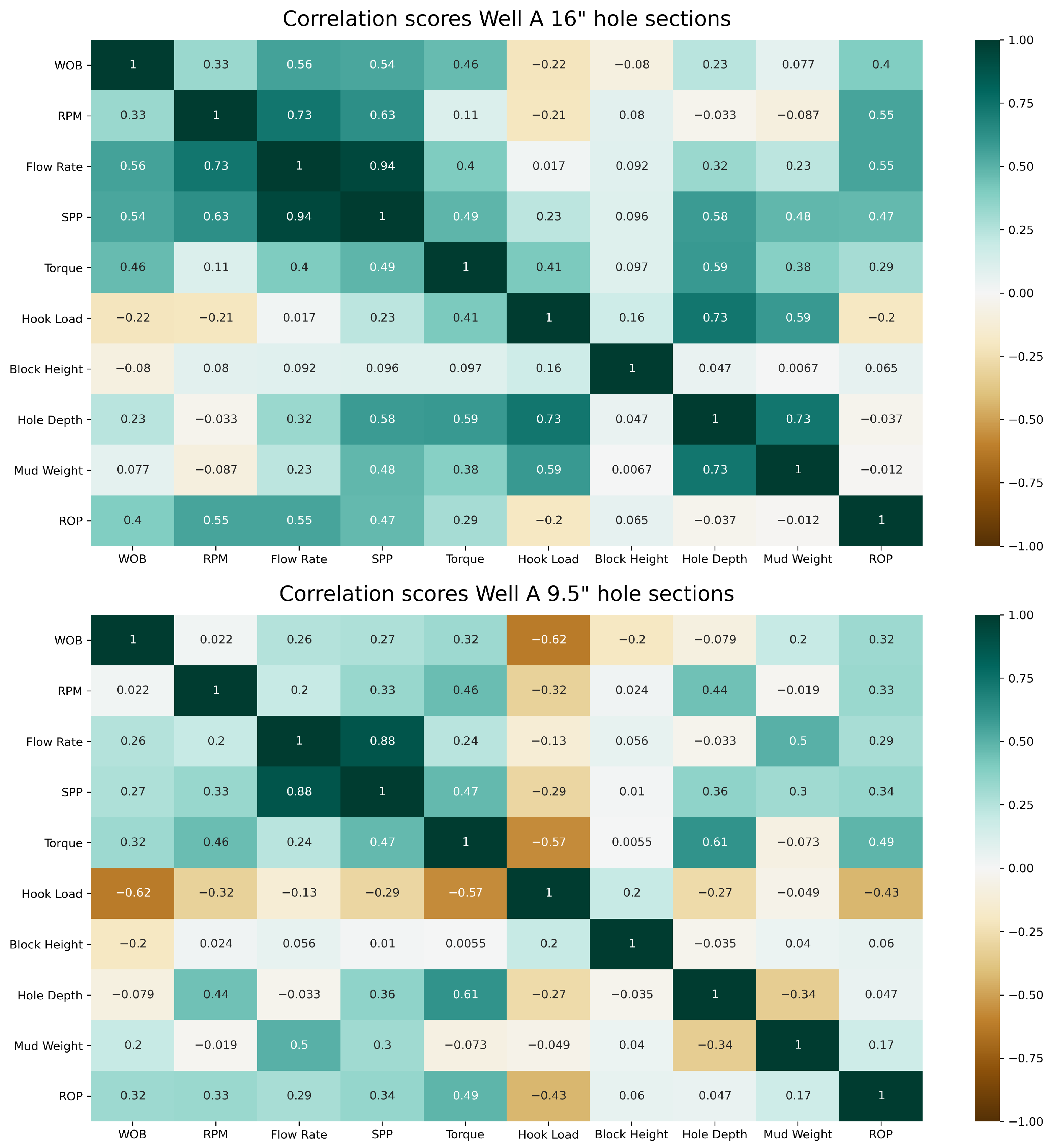
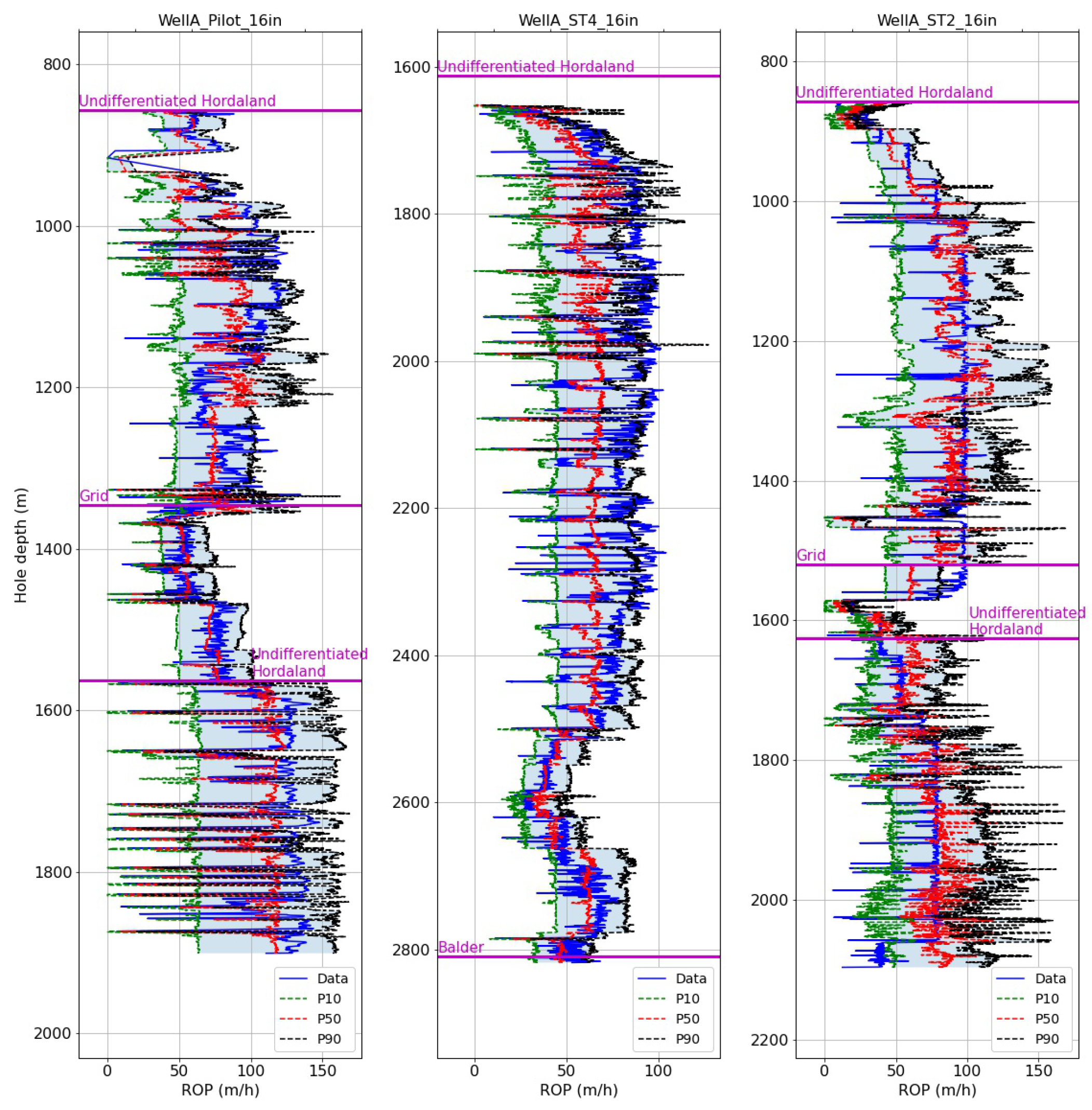
We start with the ROP predicted by models trained on Well A data sets with the hole-size-specific training strategies. In all these cases, the input feature set consists of WOB, surface RPM, surface torque and SPP, which were found to give the best results on the Well A test data sets. Figure 7 shows the depth-averaged true ROP (solid blue curve) and the predicted P10/P50/P90 (dashed curves) for the 16″ hole sections. The formation tops are annotated on the plots at the measured depths where they were encountered in each section. For the test data set (WellA_ST2_16in), the P50 curve follows the true curve quite well, and captures abrupt changes like the drop in ROP in the grid formation and around 1450 m. This results in MAE and MAPE values of of 15.7 m/h and 31.3%, respectively. The shaded light blue area between the P10 and P90 curves indicates the sharpness of the prediction, which appears wide for most of the section, spanning 100 m/h at certain depths.

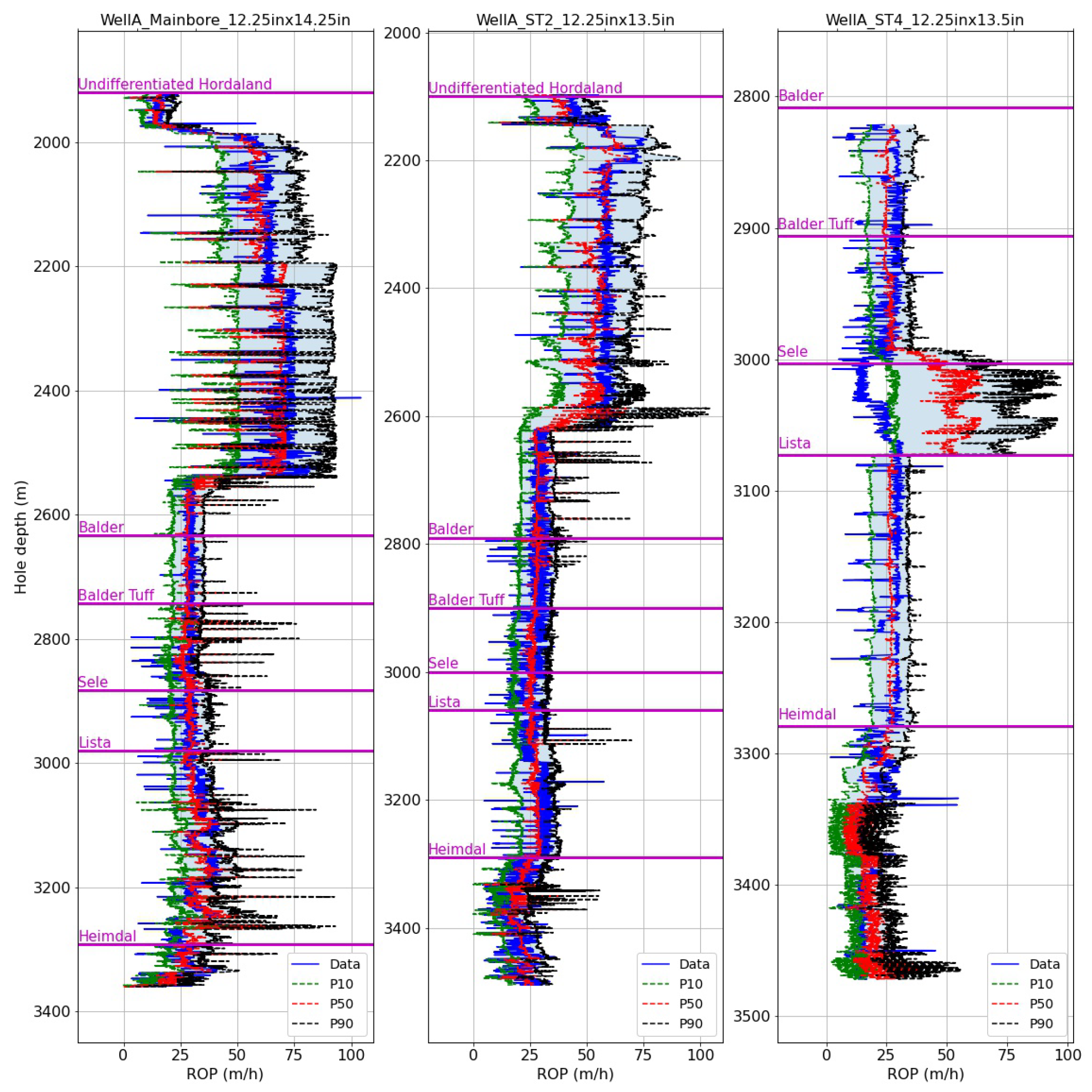
Figure 8 show the depth-averaged ROP and the predicted values for the 12.25″ sections with the hole-size-specific models. In all sections, below a depth of 2600 m, the ROP was limited to 15–30 m/h to achieve the required dogleg severity and also to deal with mud losses. The P50 curve tracks the true ROP curve very well for the training sections (WellA_Mainbore_12.25in × 14.25in, WellA_ST2_12.25in × 13.5in) and also for the test section (WellA_ST4_12.25in × 13.5in) with the exception of the Sele formation. The predictions in the Heimdal formation are close to the true ROP but quite noisy. Overall, this resulted in an MAE of 7.98 m/h and a MAPE of 43.8% for the test section.

Finally, Figure 9 displays the prediction results for the 9.5″ hole sections. The first two plots correspond to the training sections, while the last two are the test sections. The model performance is evaluated in Figure 10. The MAE and MAPE are higher on the test sections, with 10 m/h and 32.4%, respectively, for WellA_ST4_9.5in and 11.3 m/h and 56.7% for WellA_ST5_9.5in. The higher percent error for WellA_ST5_9.5in can be explained by the overall lower ROP values and reduced prediction accuracy around hard stringers compared to WellA_ST4_9.5in. The AACE for both test sections is around 10%, which is comparable to the first training section, and the sharpness is in the same range as well (24–30 m/h).

4.2. Models Trained on Formation-Specific Data

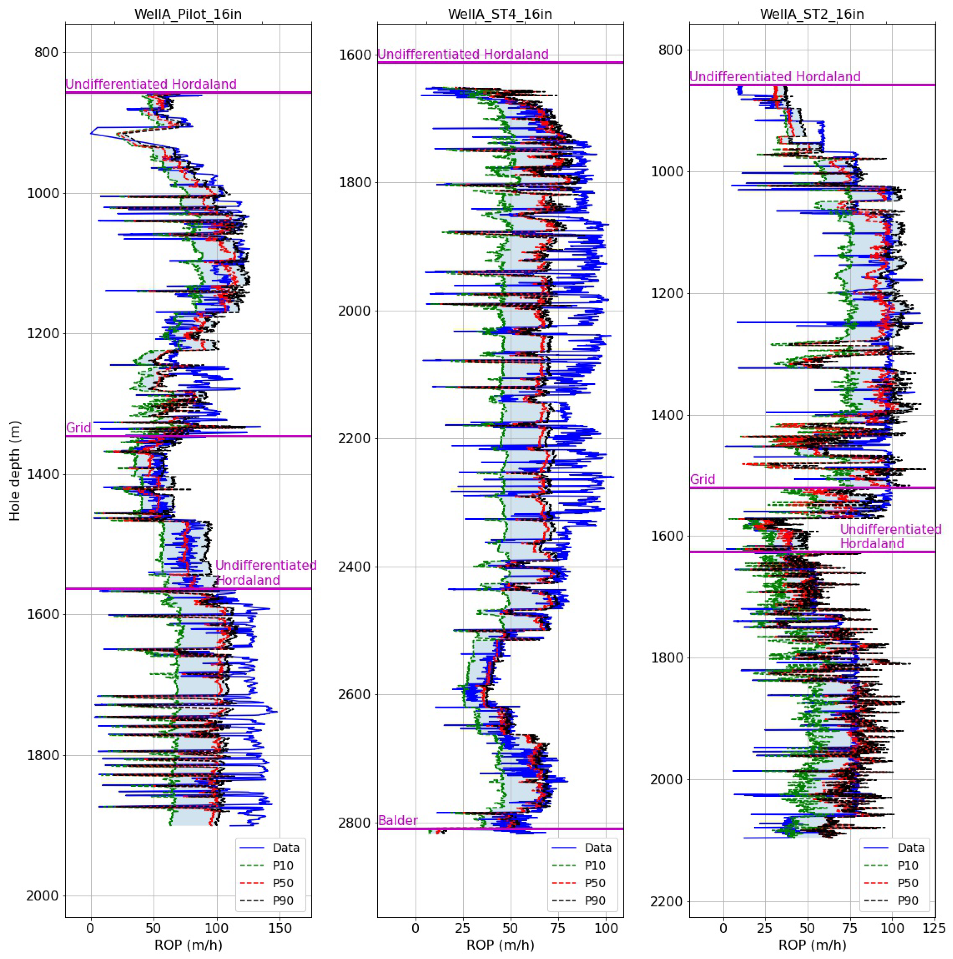
In this section, we show results for the models trained with the formation-specific strategy. As in Section 4.1, the models use WOB, surface RPM, surface torque and SPP as inputs. Figure 11 shows the results for the 16″ sections. For the test set (WellA_ST2_16in), the P50 curve follows the true curve closely for most of the section, while the span between the P10 and P90 curves is around 25 m/h. The MAE and MAPE on the test section are 13.5 m/h and 27.3%, respectively. The test set errors are notably lower than for the first training set (WellA_Pilot_16in), which achieved 19.6 m/h MAE and 29.2% MAPE with the formation-specific training strategy.

The results for the 12.25″ sections with formation-specific models are shown in Figure 12. In this case, the P50 prediction for the test section has an MAE of 6.21 m/h and a MAPE of 30.3%. This is an improvement compared to the results with the hole-size-specific strategy (Figure 8), coming mainly from the better prediction in the Sele formation. Also, the predictions with the formation-specific models are less noisy in the Heimdal formation compared to the hole-size-specific strategy. This highlights the advantage of the formation-specific training strategy, which can account for changes in the relationship between ROP and surface parameters due to differences in rock properties, whereas a model trained on an entire hole section would be less likely to capture these changes.

4.3. Comparison of Models Trained on Hole-Size-Specific and Formation-Specific Data

In this section, we compare the performance of the hole-size-specific and formation-specific models based on the four evaluation metrics. Figure 13 shows the overall performance comparison between the above training strategies on the 16″ sections. The cells are color-coded, with dark green indicating the lowest values for each metric and dark red the highest. For the test set (WellA_Pilot_16in), the MAE is lower with the formation-specific models (13.5 m/h compared to 15.7 m/h for hole-size-specific models), while the MAPE is also improved from 31.3% to 27.3%. While low AACE and high sharpness are considered better from an individual metric point of view, for the overall model performance, a balance between sharpness and AACE should be considered. With the hole-size-specific models, the test set AACE is 0.39%, while for the formation-specific models, it is 28.1%. This corresponds to a sharpness of about 24 m/h, compared to 59 m/h obtained with the hole-size-specific model. The AACE is significantly lower on the test set than on the training sets in the formation-specific case, which can be explained by the large number of ROP observations outside the P10–P90 range (see Figure 11).

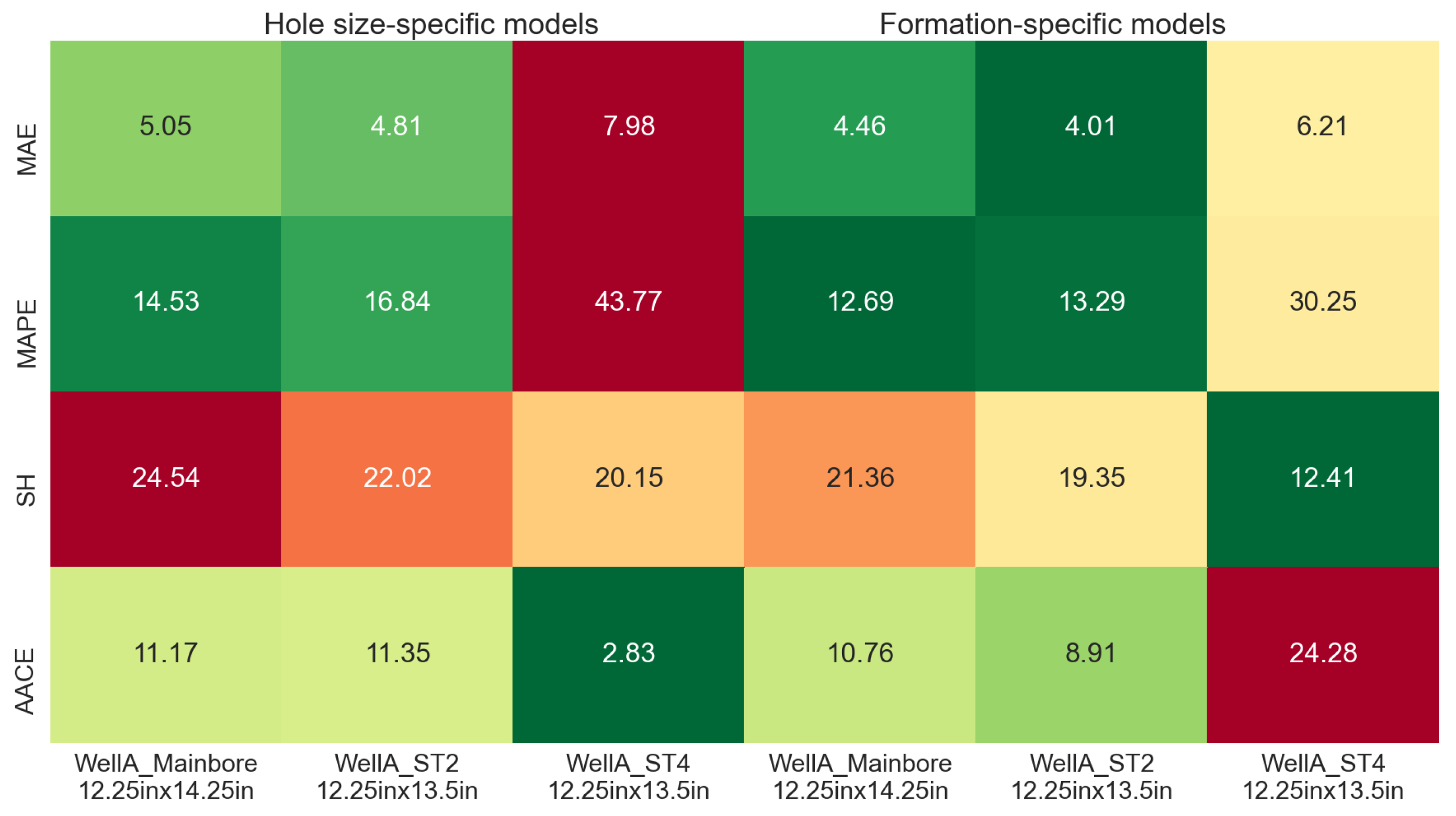
The performance of the different models for the 12.25″ sections is summarized in Figure 14. For the test set (WellA_ST4_12.25in × 13.5in), the MAE is reduced from 7.98 m/h with the hole-size-specific models to 6.21 m/h with the formation-specific models, and the MAPE is significantly improved from 43.8% to 30.3% The formation-specific strategy resulted in higher sharpness and higher AACE on the test section compared to the hole-size-specific strategy, while for the training sections, both sharpness and AACE were slightly improved, which may indicate the possible overfitting of the models.

4.4. Models Trained on Offset–Well Data

In this section, we present some results from the offset–well training strategy applied on the Well A data sets. Each model is tested on the corresponding hole sections from Well A, including 26" and 17.5", which both use the 26" hole models, since offset–well data for the 17.5" section were very limited. In addition to different offset–well groups, we also evaluate the three different input sets, as explained in Section 3.4. To provide some representative examples of how the predictions compare with different training and input sets, we choose WellA_Mainbore_12.25in × 14.25in and WellA_ST4_9.5in as the test sets. 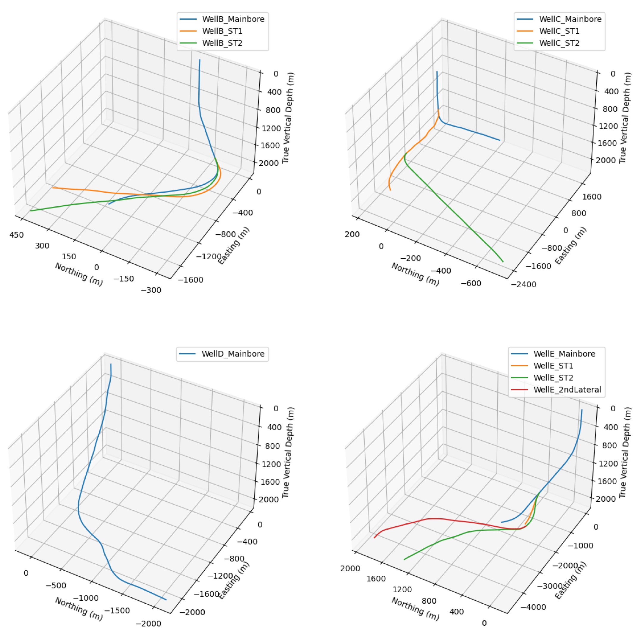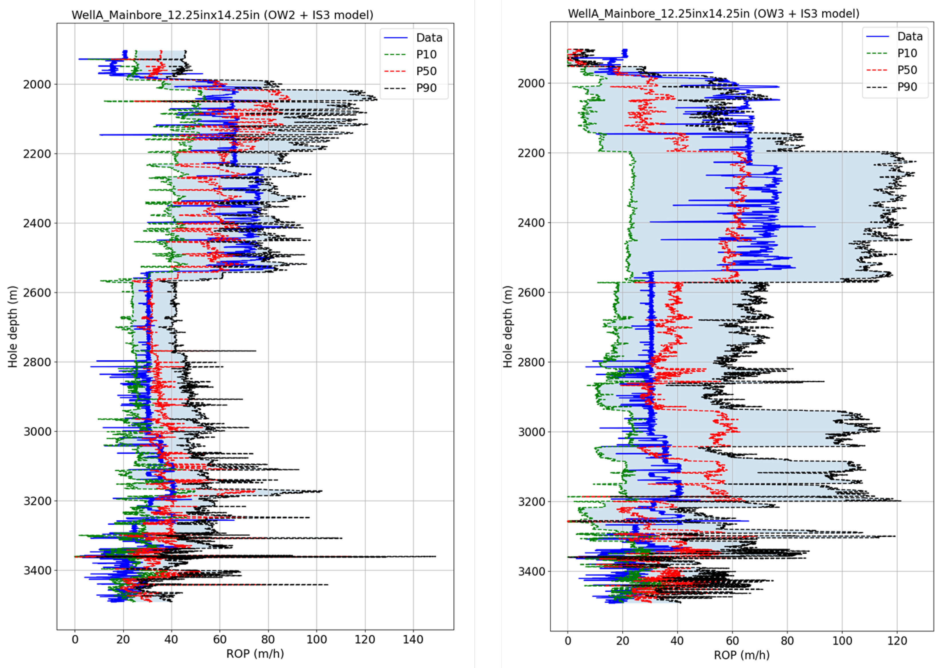Figure 15 shows the ROP predictions for WellA_Mainbore_12.25in × 14.25in with two different offset–well training sets (OW2 and OW3) for input set 3. The first combination gives the MAE of 10.1 m/h and 34.5% MAPE, while the second one gives the MAE of 14.4 m/h and 42.9% MAPE. The first model has a tighter prediction interval, corresponding to a sharpness of 31 m/h, while the second one has a sharpness of 58.6 m/h, which correspond to AACE values of 4.13% and 2.4%, respectively. These differences can be explained by having more diverse training data in OW3 compared to OW2, which introduces some uncertainty in the prediction and widens the gap between the P10 and P90 curves. The offset–well training set OW3 contains data from WellD_Mainbore_13.5in, WellE_ST1_13.5in and WellE_ST2_13.5in, while OW2 contains only data from WellE_Mainbore_13.5in, which has about three times fewer data points than the OW3 data set. Also, WellE_Mainbore_13.5in recorded less variation in the ROP than the three data sets comprising OW3 (see Table 2), and the ROP range observed in WellE_Mainbore_13.5in was closer to the one in WellA_Mainbore_12.25in × 14.25in. This can explain both the lower MAPE and narrower prediction interval obtained with the OW2 model compared to the OW3 model.

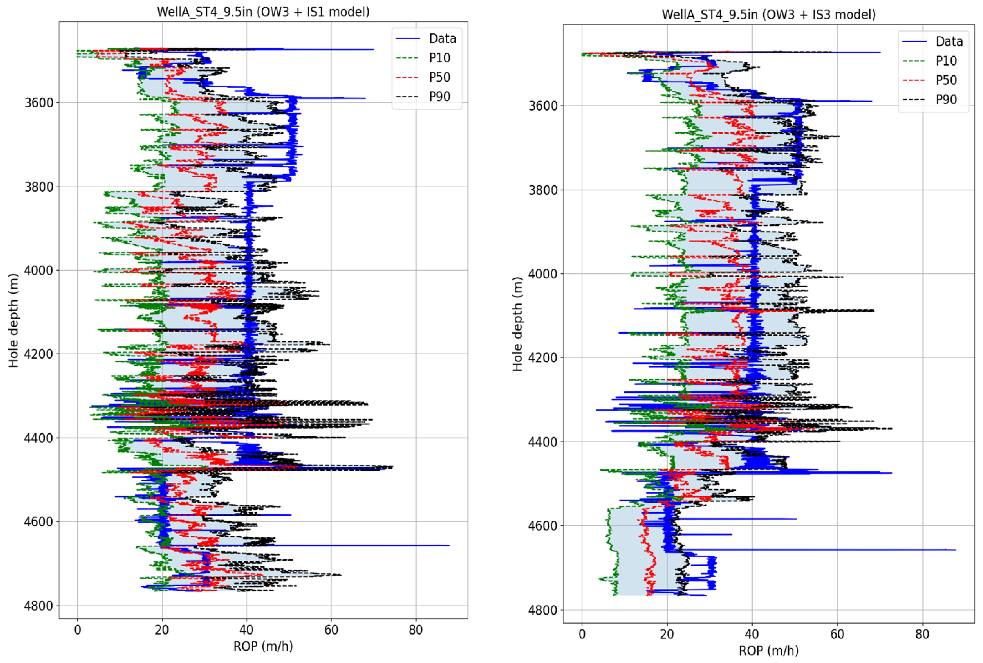
Figure 16 illustrates the ROP predictions for WellA_ST4_9.5in with the OW3 training set for input set 1 and input set 3. The first setup results in the MAE of 12.7 m/h and 36.8% MAPE, while the second one has 8.99 m/h MAE and 28.7% MAPE. The two offset–well models are comparable in terms of sharpness (21.5 m/h for the first one and 21.7 m/h), but the second one has a lower AACE at 15.1% compared to 31.5% for the first one. This can be confirmed by inspecting the plots in Figure 16, where the true ROP curve on the right plot falls within the prediction interval for most of the section, while the one on the left plot falls out of it at several depths. The improvement in coverage of the true data, as well as the reduction in MAE and MAPE, can be explained by the additional input feature used in the model training, in this case, the flow rate.

The complete evaluation for the different combinations of offset–well training sets and input feature sets is summarized in Figure A1, Figure A2, Figure A3 and Figure A4 in Appendix A, but in this section, we only provide the key findings of this study. We analyze the results separately for the upper (26″, 17.5″, and 16″), intermediate (12.25″), and lower (9.5″) hole sections. A summary of this analysis is provided in

Table 7. Offset–well ROP model performance summary. MAE and sharpness are given in m/h, MAPE and AACE is given in %.

Test Set	Best Model	MAE	MAPE	Sharpness	AACE
WellA_Pilot_26in	OW3 + IS2	21	31.7	41.8	19.7
WellA_ST4_17.5in	OW2 + IS1	11.0	50.7	17.7	17.5
WellA_Pilot_16in	OW3 + IS2	24.3	36.6	50.4	23.3
WellA_ST2_16in	OW3 + IS2	18.3	37.1	49.0	12.8
WellA_ST4_16in	OW3 + IS2	16.4	28.9	49.6	2.14
WellA_Mainbore_12.25in × 14.25in	OW2 + IS3	10.1	34.5	31.0	4.13
WellA_ST2_12.25in × 13.5in	OW2 + IS3	12.2	41.3	18.9	31.3
WellA_ST4_12.25in × 13.5in	OW3 + IS1	7.45	31.1	18.8	6.06
WellA_Pilot_9.5in	OW1 + IS3	26.2	38.4	56.7	18.2
WellA_ST4_9.5in	OW3 + IS3	8.99	28.7	21.7	15.1
WellA_ST5_9.5in	OW2 + IS1	8.55	32.2	21.1	11.3
WellA_WestLateral_9.5in	OW2 + IS3	10.8	33.0	21.5	27.2
WellA_EastLateral_9.5in	OW1 + IS2	18.8	55.1	36.1	32.7

, which indicates the best model in terms of combined accuracy and robustness for each test set and the corresponding evaluation metrics.

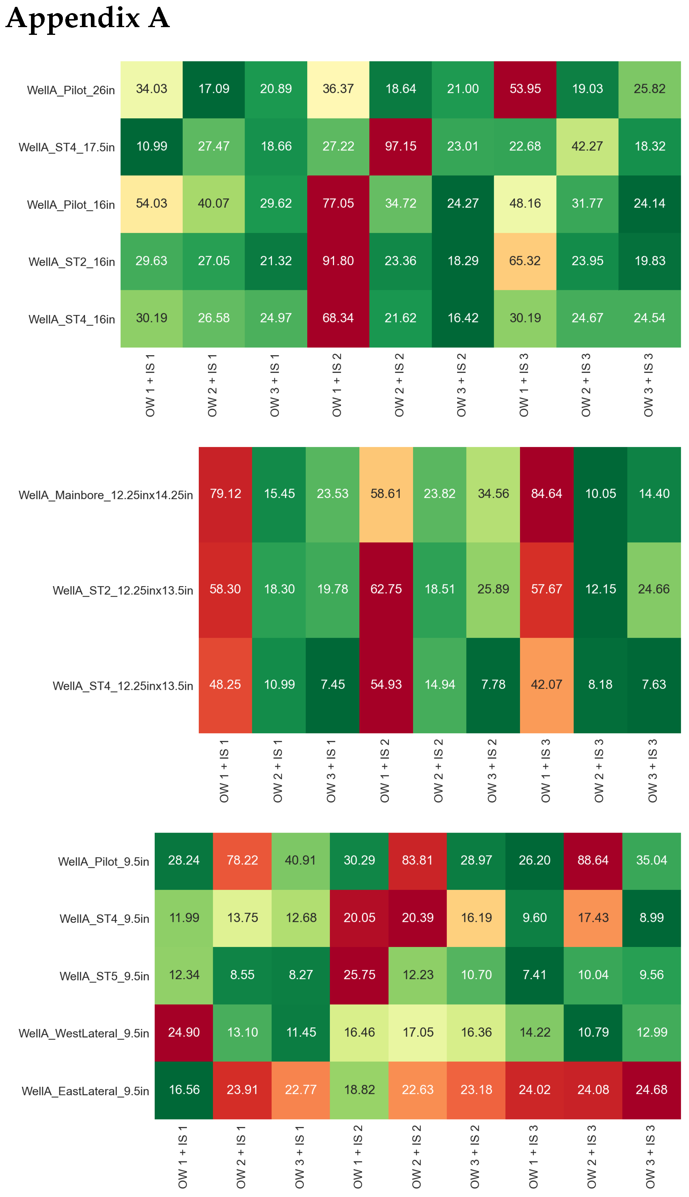
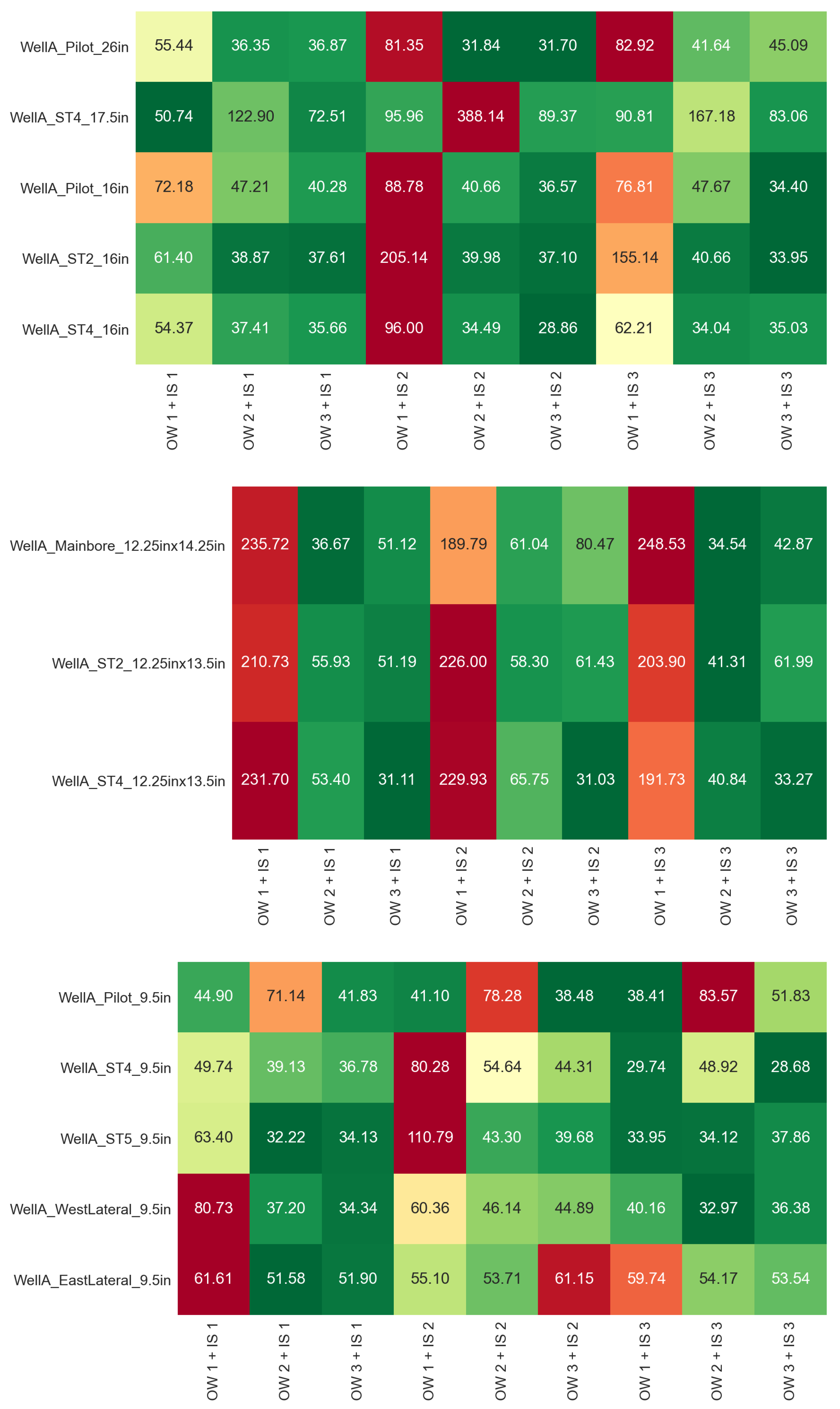
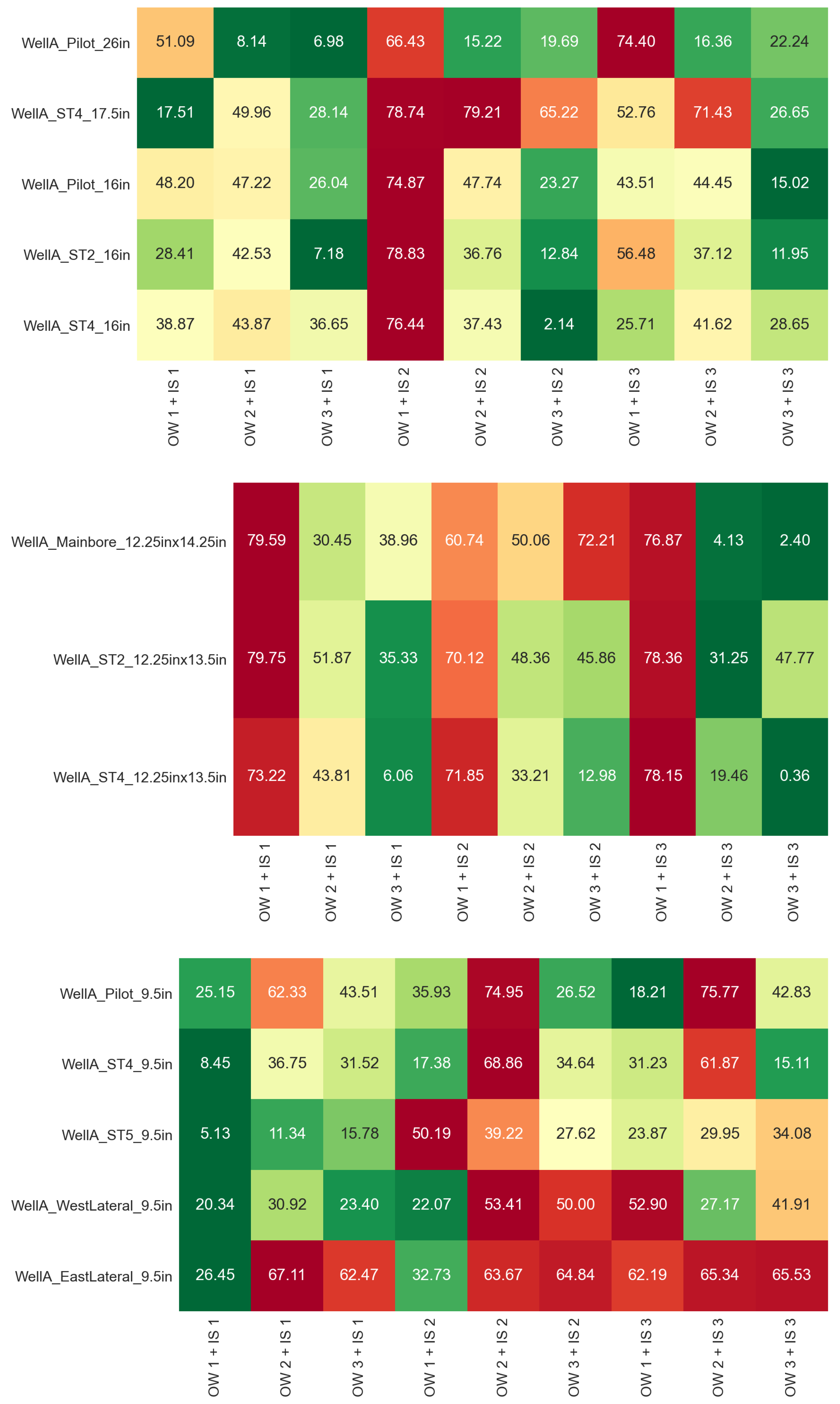
For the upper hole sections, the lowest prediction errors overall are obtained with training set OW3 and input set 2, which gives a MAPE of 31.7% for WellA_Pilot_26in, 89.3% for WellA_ST4_17.5in, 36.6% for WellA_Pilot_16in, 37.1% for WellA_ST2_16in, and 28.9% for WellA_ST4_16in. The results for WellA_ST4_17.5in are quite inaccurate in terms of MAPE (the lowest error is 50.7% with training set OW2 and input set 1), but we recall that it uses the model trained for 26″ hole data and also that part of it was drilled with a roller cone bit, which can explain the reduced accuracy. The AACE generally follows the MAPE, with values as low as 6.98% for WellA_Pilot_26in and 2.14% for WellA_ST4_16in. Regarding the sharpness of the predictions, some models produce a very narrow range of predictions, for example, training set OW1 and input set 2, having a sharpness value as low as 0.72 m/h, whereas the AACE is above 75%.

For the intermediate hole sections, the prediction errors are generally lower, with the combination of training set OW2 and input set 3 and also with training set OW3 and input set 1. The best results in terms of MAPE are 34.5% for WellA_Mainbore_12.25in × 14.25in, 41.3% for WellA_ST2_12.25in × 13.5in, and 31.1% for WellA_ST4_12.25in × 13.5in. The lowest AACE values are reported for training set OW3 and input set 3, going as low as 0.36% for WellA_ST4_12.25in × 13.5in, which is lower than the AACE obtained with the models trained on the 12.25″ hole sections from Well A. On the other hand, training set OW1 with any input combination resulted in very poor accuracy, with a MAPE in excess of 190% and also large values of AACE, despite having low sharpness. These large errors can be explained by the fact that all the intermediate sections in Well A, training set OW2 and training set OW3 were drilled with an under-reamer, whereas the ones in training set OW1 did not use an under-reamer, which likely resulted in different drilling performance. The sharpness for the best-performing models is in the range of 13–25 m/h, which is similar to the range observed for the 12.25″ sections trained on Well A data.

For the lower hole sections (9.5″), there is no single model that outperforms the other ones in terms of combined accuracy and robustness. The best models result in a MAPE of 38.4% for WellA_Pilot_9.5in, 28.7% for WellA_ST4_9.5in, 32.2% for WellA_ST5_9.5in, 33.0% for WellA_WestLateral_9.5in and 55.1% for WellA_EastLateral_9.5in. For WellA_ST4_9.5in and WellA_ST5_9.5in, these results show an improvement compared to the model trained on the Well A 9.5″ sections themselves. 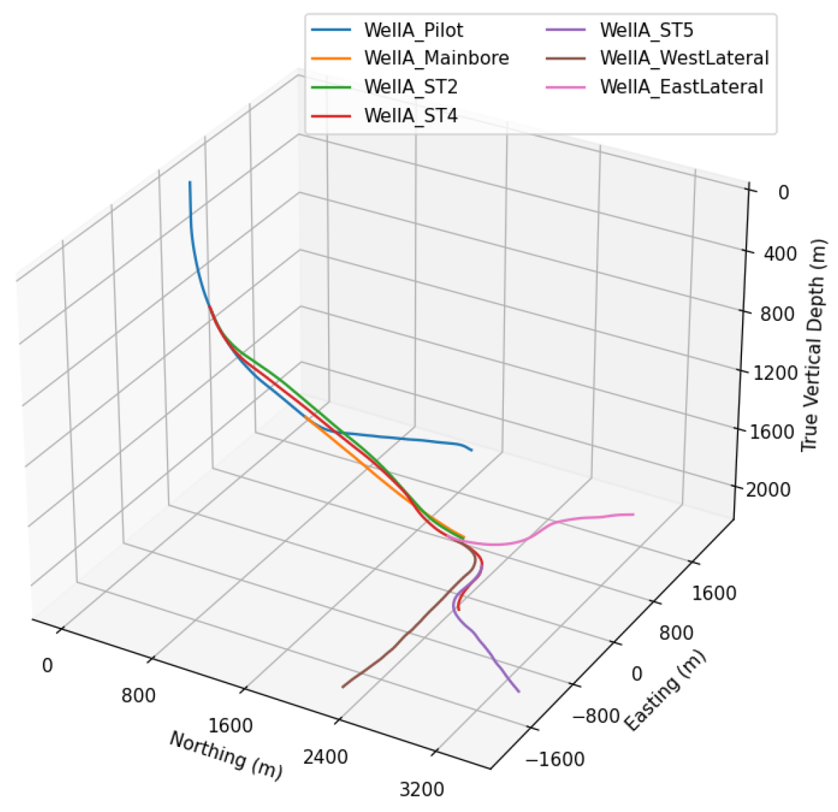Even for the other training set and input combinations, the MAPE stays below 50% for most cases, which can be considered within reasonable accuracy according to [55]. Regarding the AACE, the combination of the training set OW1 and input set 1 achieved the lowest values overall (8.45% for WellA_ST4_9.5in and 5.13% for WellA_ST5_9.5in), but this comes with a higher MAPE and reduced sharpness. The majority of 9.5″ section models trained on offset wells have a sharpness around 15–20 m/h, compared to 24 m/h and above, which was reported for the model trained on Well A. Comparing this against AACE, it can be concluded that a sharpness around 20–30 m/h is preferable as it generally results in lower AACE for the 9.5″ hole sections. Some of the worst results, in terms of both MAPE and AACE, are recorded for WellA_PilotA_9.5in, which stands out among all the 9.5″ hole sections due to its larger overall ROP and different well inclination (see Table 1 and Figure 2). Also, the MAPE and AACE reported on WellA_EastLateral_9.5in are on average very high, which could be due to the presence of hard stringers and vibrations that may cause very different downhole conditions from the ones in the training sections, which affects the relationship between ROP and the surface drilling parameters. Therefore, it may be preferable to use this entire section or at least part of it for training the ROP model, as in Section 4.1.

5. Discussion

Data-driven models for ROP prediction rely on large amounts of training data, either from different sections of the same well or from the nearby offset wells. Our model, based on the offset–well data, achieves predictions with good accuracy and robustness. As mentioned above, the presence of downhole vibrations may impact the relationship between ROP and the surface drilling parameters, leading to prediction errors. To improve model performance, inputs from downhole mechanical measurements (e.g., RPM, WOB, and torque measured in the BHA) could be added to the ROP model for wells where such downhole measurements are available. Another source of prediction error can be related to the geological and mechanical parameters of the rock formations drilled, which were not available from the drilling operation reports analyzed as part of our study. With the formation-specific training strategy, this error was reduced, but possible uncertainty related to the depth where a formation is encountered across different wells can also contribute to the prediction errors. In addition, short, hard stringer intervals interbedded in a softer formation are difficult to capture in the training data. If rock mechanical parameters are available, it would be possible to identify the hard stringers and use a separate ROP model training strategy for the intervals containing hard stringers.

In our study, we observed that not all offset–well data are relevant or useful for training the model. To ensure that the model is accurate and reliable, it is important to carefully select the offset–well data that are used for training the ROP models. ML and similarity analysis can help in the selection of representative training data sets.

One criterion that can be considered in this selection process is the distance to the target well, such that the model is trained on data that are geographically relevant, and similar lithologies are encountered during the drilling process. Lithology information can further improve the training, but if it is available, the uncertainty in the formation tops should be taken into account. Another criterion is to select offset wells that were drilled during a similar time period, as the target well can ensure that the model is trained on data that are more relevant to the current drilling conditions and operational practices. Selecting offset–well sections that have a similar well trajectory and orientation (vertical/inclined/horizontal) to the target well can also help improve the model quality.

The type of drill bit used (polycrystalline diamond compact, roller cone, or hybrid bit) and other downhole equipment (e.g., under-reamer, rotary steerable system, or downhole motor) should be the same as in the target well. The drilling platform type should also be similar, particularly for offshore drilling, where rig heave can have a significant impact on the drilling process and sensor readings. Here, the information on whether an active or passive heave compensation system is present could also be relevant. Finally, the selection process should prioritize offset wells that did not experience any drilling incidents, such as high levels of vibration, drill bit damage, stuck pipes or lost circulation, such that the model is trained only on data that are representative of normal drilling conditions. On the other hand, those wells or sections can be used to train dedicated models accounting for degradation in drilling conditions, for example, ROP models corresponding to different degrees of bit wear, which could be used to detect bit wear from real-time data in the target well.

Further work on this topic should explore the application of the QRDNN model in the context of data-driven drilling optimization by using the model predictions with the provided measure of confidence to aid in the selection of drilling parameters that maximize ROP while staying within operational constraints.

6. Conclusions

We presented an application of quantile regression deep neural network (QRDNN) models for the prediction of the rate of penetration (ROP) in a multi-lateral well drilled in the North Sea. Given the highly uncertain conditions of offshore drilling over several kilometers, QRDNNs provide not only a best-guess prediction (the median) but also an uncertainty range (from P10 to P90), offering valuable insight into potential variations in drilling performance without any additional calibration.

We analyzed the sensitivity of the results to inputs: a feature set comprising WOB, surface RPM, surface torque, and flow rate yielded the best performance in most cases. However, the primary focus was training data selection for the QRDNN model to balance accuracy and robustness. Three training strategies were evaluated based on hole size, formation tops, and offset–well data. The key quantitative findings are as follows:

• The hole-size-specific training strategy produced accurate predictions on the training sets, but the mean absolute percentage error (MAPE) on test sets from the same well was relatively high, with a MAPE of 31.3% on the 16″ hole section, 43.8% on the 12.25″ section, and 32.4% and 56.7%, respectively, on two 9.5″ hole sections. On the other hand, the absolute average coverage error (AACE) was below 10% for all the test sections evaluated.
• The formation-specific training strategy reduced the MAPE, producing a result of 27.3% for the 16" test section and 30.3% for the 12.2" test section. At the same time, the AACE increased above 24% for both test sections due to narrower prediction intervals (outer-quantile overfitting) compared to the first strategy.
• The offset–well training strategy achieved a MAPE as low as 31.7% for the test well 26″ hole section, 28.9% for the 16″ hole sections, 31.1% for the 12.25″ hole sections, and 28.7% for the 9.5″ hole sections. The observed AACE was also low: 6.98% for 26″, 2.14% for 16″, 0.36% for 12.25″, and 5.13% for 9.5″ hole sections respectively. We observed that the inclusion of more offset wells in the training set reduced the MAPE and AACE and estimated more uncertainty in the predictions.

Thus, we recommend the offset–well training strategy for QRDNN-based ROP prediction. Within this approach, including more offset wells in the training set ensures lower prediction errors and better uncertainty estimation. This combination provides both accurate predictions and a quantifiable measure of confidence, making QRDNNs a valuable data-driven tool for drilling performance optimization.