Design and Analysis of a Quasi-Biaxial Solar Tracker

Abstract

Inspired by C. Alexandru, to achieve a balance between tracking accuracy and equipment cost and between single-axis tracking brackets and dual-axis tracking brackets, a kind of quasi-biaxial solar tracker, whose approximate two-axis motions are driven by a single motor, is studied in this paper. Firstly, considering the changes in the total number of sunny days and declination angle in a certain period of time, the characteristic day of the tracker in this period is set. Then, based on the variations in the Sun’s azimuth and elevation angle on the characteristic day, a quasi-biaxial solar tracker mechanism is designed. Its azimuth angle movement is directly driven by a single motor, while the elevation angle movement is driven by the same motor through a bevel gear and a cam mechanism. The solar irradiance of the photovoltaic module of the solar tracker is analyzed using PVsyst software. Through 3D modeling-aided design, a prototype of the solar tracker is built and then relative experiments are conducted to study the performance of the quasi-biaxial solar tracker. Simulation analysis and physical model experiments show that the quasi-biaxial solar tracker works and achieves a relative compromise between tracking accuracy and cost.

1. Introduction

With the depletion of traditional fossil energy sources and growing environmental concerns [1,2,3], the search for clean, sustainable energy sources is urgent. As global energy demand continues to increase, renewable energy’s competitiveness is rapidly improving. Research shows that it is expected to account for half of global energy use in 2035, and the energy mix will continue to decarbonize [4]. Solar energy is a type of energy generated by solar radiation [5], which is increasingly being emphasized due to its non-polluting and sustainable generation. Solar energy can be used to generate thermal energy or it can be converted into electricity through photovoltaic (PV) systems [6]. When sunlight hits a photovoltaic module, photons excite electrons in the semiconductor material, prompting them to move, which creates an electric current [7]. Solar photovoltaic (PV) technology is now playing an important role in a number of fields, and building-integrated photovoltaic (BIPV) technology, in particular, has considerable potential in the utilization of solar energy [8,9,10,11,12]. The strength of the current generated by a photovoltaic module depends greatly on the amount of solar radiation energy it receives. Therefore, PV brackets play an important role in improving the yield of PV power generation systems. By using PV brackets, the PV modules can be maximized to be perpendicular to the incident light from the sun, and the power generation efficiency of the PV modules can be improved.

In order to enhance the power generation efficiency of photovoltaic modules, many scholars have carried out a large number of in-depth research in the field of photovoltaic power generation since Finster [13] designed a mechanical solar tracking system in 1962. In 1975, McFee [14], in an effort to increase the efficiency of energy harvesting per unit of time, proposed a new tracking system that utilized a central collector to gather the light concentrated by the surrounding reflector units and determine the position of the sun based on the data reflected by each reflector unit. Abdallah et al. [15] designed an open-loop, programmable logic controller-controlled, dual-axis solar tracking bracket that increased the solar irradiation energy received by the PV modules by 41.34% compared to a fixed bracket oriented in a due south direction with a tilt angle of 32°. Song et al. [16] designed a dual-axis tracking bracket system based on a fiber optic composition, which consists of two feedback loops that utilize an angle encoder and a specific array of wide-area diodes for angular adjustment, resulting in a tracking accuracy error of the PV module within 0.1°. Gabe et al. [17] designed a two-axis tracking bracket system consisting of a mechanical structure and an electrical system, which was utilized to accurately determine the position of maximum solar radiation even under cloudy weather conditions using the system’s control logic. The current status, constraints, and future trends of the sustainable development of solar photovoltaic (PV) tracking technology have been studied by Yang Zihan et al. [18]. The results of these studies not only enhance the economic efficiency of solar tracking systems but also their environmental adaptability [19,20,21,22,23]. However, of the many designs, almost all of them are to improve the tracking accuracy in the working process to increase additional revenue, and there are few articles directly targeting the optimization design of PV bracket construction cost. The reason for this is that the PV tracking bracket structure can be optimized in a small space, and the relevant design manuals can be referenced to a single form of design.

PV brackets can be categorized into fixed brackets [24], single-axis tracking brackets [25,26], and dual-axis tracking brackets [27] according to the number of rotating axes [28,29,30]. Compared with fixed brackets, single-axis tracking brackets usually only track changes in solar azimuth or elevation angle, and can obtain an additional 10–25% power generation gain on the basis of only a 7–10% increase in investment [17,31,32]; dual-axis tracking brackets can track changes in solar azimuth and elevation angle at the same time, which significantly improves the power generation gain, but the cost is also relatively high [33,34,35,36,37].

Aiming to seek a balance between the power generation efficiency of PV systems and system cost, C. Alexandru proposed a single motor-driven dual-axis solar tracking mechanism [38], and its simulation analysis shows that this bevel gear-cam type mechanism can produce an effect close to dual-axis tracking, and the solar radiation received by its PV modules will be significantly higher than that of fixed PV brackets but lower than that of a dual-motor-driven dual-axis tracking system, characterized by minimizing the use of drive motors and achieving a certain balance between tracking effect and equipment cost, but the study does not give the verification results of the physical system. Inspired by it, this paper carries out the design, simulation, and analysis of a single-motor-driven quasi-biaxial PV bracket system, which is a solar tracking mechanism that can be driven by a single motor. It utilizes a mechanical transmission to achieve the simultaneous tracking of PV modules to the sun’s azimuth and elevation angles, and experimental validation is carried out.

2. Design Principle of the Quasi-Biaxial Solar Tracker

According to the movement law of the sun, combined with the movement form and characteristics of the dual-axis tracking bracket, a new type of solar tracking bracket is proposed [38], which utilizes a mechanical transmission device to replace the motor that drives the rotation of the elevation axis, and realizes the simultaneous tracking of the PV module to the sun’s azimuth angle and elevation angle by a driving motor. In this paper, this tracking bracket mechanism is called quasi-biaxial and its design principle is given in this section.

Every day, the sun rises in the east and sets in the west due to the rotation of the Earth. From the heliocentric theory, it can be seen that the Earth is rotating around the Sun. In order to facilitate people the analysis of the Sun’s motion, this paper assumes that the Sun is around the Earth in a circular motion, as shown in Figure 1, and this circular motion is called the Sun’s apparent motion. To specifically describe the position of the Sun, the Sun’s position is usually labeled using the Sun’s azimuth $\gamma$ [39] and elevation angles $\alpha$ [40], where azimuth is 0° to the due south, negative to the east, and positive to the west [39]. Therefore, the PV tracking bracket needs to track the changes in solar azimuth angle and solar elevation angle, respectively, to realize the accurate tracking of the PV module to the Sun’s position [41].

The solar elevation angle $\alpha$ is calculated by the following formula [40]:

$$\sin \alpha =\sin \delta \cdot \sin \phi +\cos \phi \cdot \cos \omega$$

(1)

The solar azimuth angle $\gamma$ is given by [39]

$$\sin \gamma ={\displaystyle \frac{\cos \delta \cdot \cos \omega }{\cos \alpha }}$$

(2)

where $\phi$ is the local latitude [40] and $\delta$ is the angle of declination, which is the angle of the line between the Sun and the center of the Earth and the plane of the equator, as specified by the following formula [42,43]:

$$\delta =0.3723+23.2567\sin \theta +0.1149\sin 2\theta -0.1712\sin 3\theta -0.758\cos \theta +0.3656\cos 2\theta +0.0201\cos 3\theta ,$$

(3)

where $\theta ={\displaystyle \frac{2\pi (n-n_0)}{365.2422}}$, $n$ is the accumulation day [21].

$\omega$ is the time angle and is calculated as [40]

$$\omega =(S-{\displaystyle \frac{4\times (120-jd)}{60}}+{\displaystyle \frac{E_t}{60}}-12)\times 15$$

(4)

$S$ is Beijing time and $jd$ is the longitude of the location. $E_t$ is the time difference, calculated as [44]

$$E_t=0.0028-1.9857\sin \theta +9.9059\sin 2\theta -7.0924\cos \theta -0.882\cos 2\theta$$

(5)

$\theta$ in Equation (5) is the same as the formula for $\theta$ in Equation (3).

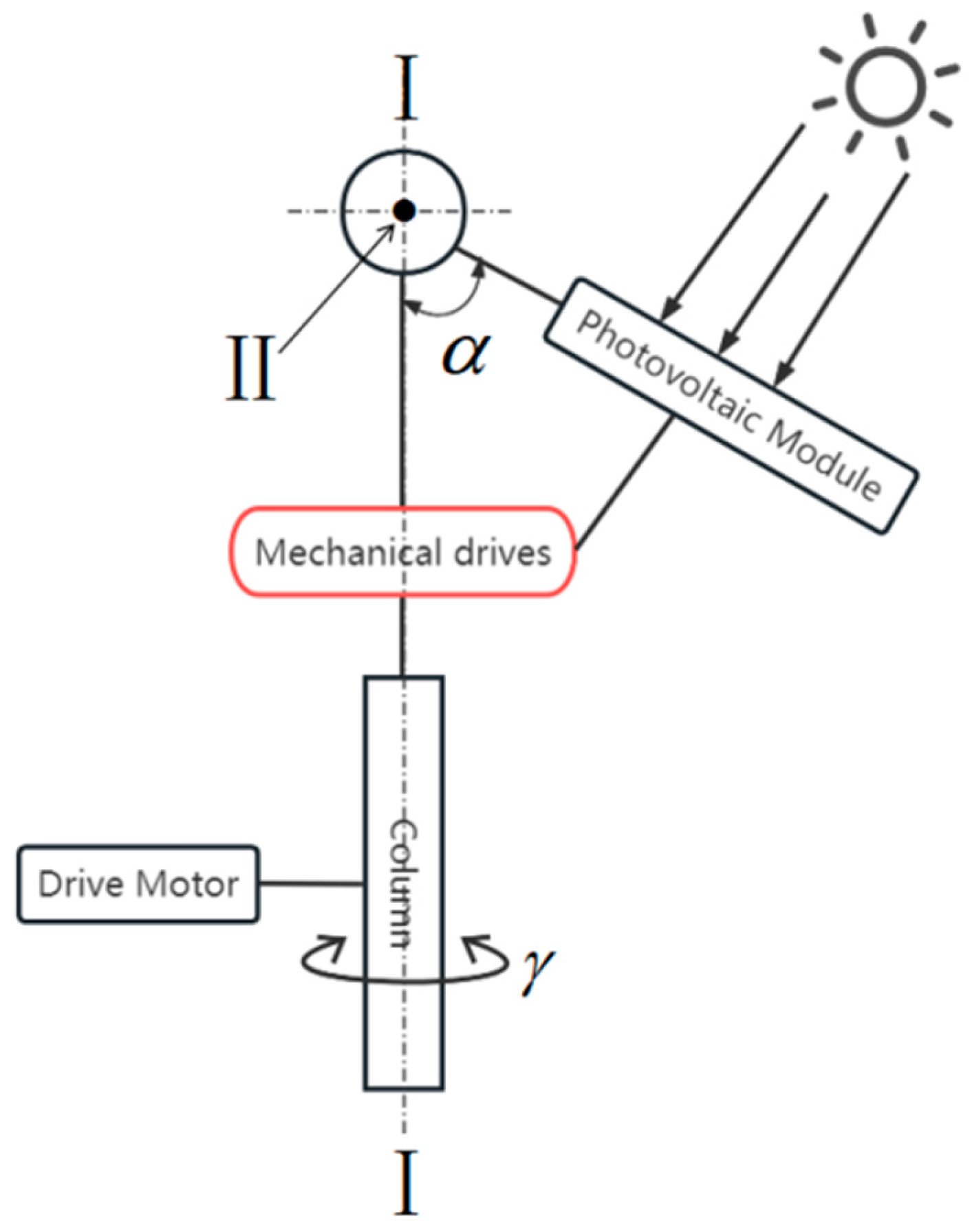
The structural principle schematic of the quasi-biaxial solar tracker shown in Figure 2 takes the azimuth dual-axis tracking system as the design model [45], and its main motion axis is perpendicular to the ground, which provides good stability for the overall structure. By setting motor 1 as the power source of the overall device, the photovoltaic module is driven to rotate horizontally by means of time control to realize the tracking of the azimuth angle of the sun by the photovoltaic module; at the same time, a mechanical transmission device is used to replace the motor that drives the elevation axis, so as to realize the tracking of the Sun’s elevation angle by the photovoltaic module.

Its azimuth axis $Ⅰ$ and elevation axis $Ⅱ$ have the following main characteristics when tracking the Sun:

(1)

The spatial positions of the azimuth and elevation axes are perpendicular to each other: $Ⅰ\perp Ⅱ$;

(2)

The angular speeds of rotation of the azimuth and elevation axes are different: ${\omega }_{Ⅰ}\ne {\omega }_{Ⅱ}$;

(3)

The azimuth and elevation axes rotate according to the azimuth and elevation angles of the Sun, respectively, and the rotation range of the azimuth axis is much larger than that of the elevation axis: ${\theta }_{Ⅰ}>{\theta }_{Ⅱ}$.

The azimuth and elevation axis have the same rotation period: $T_{Ⅰ}=T_{Ⅱ}$.

The pattern of the Sun’s movement throughout the year is as follows: in the spring the Sun is located near the equator; in the summer the Sun is located between the equator and the meridian of the inner return; in the fall the Sun is once again located near the equator; and in the winter the Sun is located between the equator and the meridian of the southern return. The Sun, centered on the equator, sweeps back and forth between the Tropic of Cancer and the Tropic of Capricorn, once a year, in a continuous cycle that creates the phenomenon of sequential alternation of seasons on Earth throughout the year. Due to the Sun’s different daily declination angles and the differences in the formulae for calculating total and direct irradiance on clear days, the Sun’s elevation angle is different every day, adding difficulties to the design of the mechanical drive and placing higher demands on the tracking control system [46,47,48].

In order to simplify the tracking system, the year is divided into several time periods with similar solar path characteristics based on the changing pattern of the total number of clear-sky radiation days. For a certain period of time, calculate the average value of the Sun’s declination angle for all the days in the period of time, select the day in the period of time when the Sun’s declination angle is closest to the average value as the “characteristic day” in the period of time, and use the rule of change of the Sun’s elevation angle of that day to represent the change of the Sun’s elevation angle of each day in the whole period of time.

The theoretical light intensity of the Sun at a given time can be calculated from the Belyand theoretical equation, which is given as [49,50,51]

$$I={\displaystyle \frac{I_{sc}\cdot {\sin }^2\alpha }{f+\sin \alpha }}$$

(6)

where $I_{SC}$ is the solar system number of size: $I_{SC}=1367\pm 7\begin{array}{}\end{array}{\mathrm{W}/\mathrm{m}}^2$; $\alpha$ is the solar elevation angle; $f$ is the Castroff coefficient, which is determined by the state of atmospheric transparency and is used to characterize the effect on the amount of radiation as the content of the different components of the atmosphere varies. On an ideal clear day with good atmospheric transparency, the $f$-value varies less during the day and can be considered to be constant, as specified in the following formula [21]:

$$f=0.133+0.084\times \ln (1+e)$$

(7)

where $e$ is the local ground water vapor pressure.

Let $A=\sin \delta \cdot \sin \phi$, $B=\cos \delta \cdot \cos \phi$; then, Equation (1) is $\sin \alpha =A+B\cdot \cos \omega$, which is brought into Equation (6), and the total number of sunny radiant days in a day’s time can be obtained by integrating over time [52,53].

Using $dt={\displaystyle \frac{T}{2\pi }}\cdot d\omega$ to convert time differentiation into diagonal differentiation, we have

$${\displaystyle {\int }_{t_1}^{t_2}Idt={\displaystyle {\int }_{{\omega }_1}^{{\omega }_2}Id\omega }}$$

(8)

where ${\omega }_1$ and ${\omega }_2$ are the time angles at the beginning and end of a time period, respectively, and when ${\omega }_1=-\arccos (\tan \delta \cdot \tan \phi )$ and ${\omega }_2=\arccos (\tan \delta \cdot \tan \phi )$, the equation is the formula for calculating the total daily value of total radiation on a clear day.

The division of the time period and the selection of the characteristic days take into account two main factors: the total number of sunny radiation days and the angle of declination. Based on the relationship between the total number of radiant days and the angle of declination on a clear day, combined with the formula for the angle of declination, the equation for the relationship between the total number of radiant days and cumulative days is expressed as follows [54]:

$$H_{(N)}=a+b\cdot \sin ({\displaystyle \frac{2\cdot \pi \cdot n}{365}}-d)$$

(9)

The total number of sunny radiation days in a year is obtained by using Equation (8), and the values of parameters $a$, $b$, and $d$ in Equation (9) are solved based on the values obtained from the calculation results, and then substituted into Equation (9), which is the relationship equation between the total number of sunny radiation days and the cumulative number of days.

For example, the total number of sunny radiant days in a year is divided into three intervals corresponding to the four seasons of the year: spring, summer, fall, and winter, with spring and fall as one interval, located between the summer months of winter. The specific segmentation nodes are as follows:

$$H_{(14)}=H_{(\min )}+(1-{\displaystyle \frac{\sqrt{2}}{2}})\times {\displaystyle \frac{H_{(\max )}+H_{(\min )}}{2}}$$

(10)

$$H_{(23)}=H_{(\max )}-(1-{\displaystyle \frac{\sqrt{2}}{2}})\times {\displaystyle \frac{H_{(\max )}-H_{(\min )}}{2}}$$

(11)

where $H_{(\max )}$ is the maximum value of the total number of sunny radiation days in a year and $H_{(\min )}$ is the minimum value.

As shown in Figure 3, when $H_{(n)}=H_{(14)}$, the corresponding product days $n_1$ and $n_4$ are solved, and when $H_{(n)}=H_{(23)}$, the corresponding product days $n_2$ and $n_3$ are solved. The year was divided into four time periods based on the resulting product days: $n_1\to n_2$, $n_2\to n_3$, $n_3\to n_4$, and $n_4\to n_1$ of the second year, and the mean value of the angle of declination within each time period was calculated, and the day with the angle of declination closest to the mean value within the time period was used as the characteristic day of the time period.

3. Structural Design of Quasi-Biaxial Solar Tracker

The overall structure is shown in Figure 4, including an azimuth angle tracking mechanism and an elevation angle tracking mechanism, which mainly consists of parts such as a 1—bracket base; 2—drive motor; 3—column; 4—beam; 5—photovoltaic module frame; 6a, 6b—bevel gear; 7—fixed support guide bearing; 8—drive shaft; 9—cam; 10—cam follower; 11—cam follower fixing support, and so on. While in the bracket base 1 provides good stability for the overall device; the drive motor 2 is fixed inside the bracket base 1, and the output shaft of the drive motor 2 passes through the opening at the top of the bracket base and is connected to the column 3 via a flange coupling; the beam 4 is connected to the column 3 via a two-way connector fixture; the beam 4 is fitted with a pin holder, which is connected to the photovoltaic module frame 5 by means of a pin, and the photovoltaic modules are mounted on the photovoltaic module frame 5; a fixed support guide bearing 7 is bolted to the side of the column 3; the drive shaft 8 is connected to the fixed support guide bearing 7 by means of an interference fit, and a keyway is provided on the drive shaft 8, and the vertical bevel gear 6b and the cam 9 are fixed to the drive shaft 8 by means of a key connection and a shaft-end retaining ring; the horizontal bevel gear 6a is in contact with the upper-end surface of the bracket base 1 by means of its own gravity and is fixed to the bracket base 1 by means of a key connection; and the cam follower 10 is held by the cam follower fixing support 11 restricting its 5 degrees of freedom so that the cam follower 10 can only slide axially within the end fixing ring of the cam follower fixing support 11; one end of the cam follower 10 is connected to the contoured surface of the cam 9, and the other end slides on the backside of the photovoltaic module frame 5 by means of a roller. In the azimuth tracking mechanism, the photovoltaic module frame is directly connected to the drive motor through the beam and column, and the drive motor drives the photovoltaic group frame to rotate horizontally, realizing the tracking of the Sun’s azimuth angle. The elevation angle tracking mechanism is mounted on the side of the column, through the bevel gear mechanism and cam mechanism, to realize the PV module to the Sun’s elevation angle tracking. A fixing bracket is provided in the center of the cam follower to support the cam follower and limit its degrees of freedom. The drive motor operates in conjunction with the bevel gear mechanism and cam mechanism to enable the PV module to track the Sun’s azimuth angle while tracking the Sun’s elevation angle.

According to the motion characteristics of the tracking bracket and the tracking principle, the design of the mechanical transmission device needs to meet the following requirements at the same time:

(1)

The azimuth axis needs to generate an additional motion in the vertical direction to power the rotation of the elevation axis as it rotates horizontally;

(2)

The mechanism causes the photovoltaic module to produce a rotation of the elevation axis that needs to be less than the rotation of the motor-driven azimuth axis;

(3)

The mechanism needs to change the rotational speed of the azimuth axis to the desired rotation speed of the elevation axis;

(4)

The azimuth and elevation axes need to start and finish work at the same time.

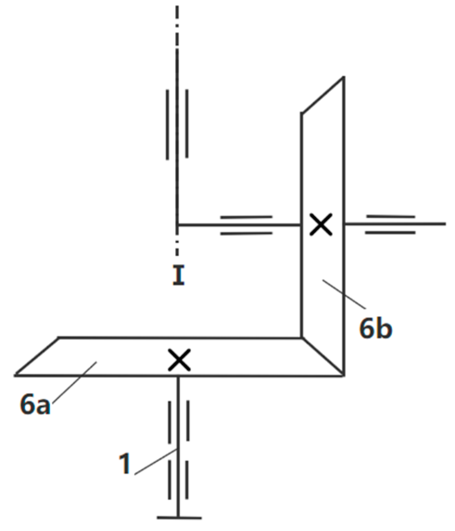
Figure 5 shows a sketch of the movement of the bevel gear mechanism, wherein the use of the bevel gear transmission mechanism can rack the horizontal rotation of the bracket at the same time and additionally obtain a vertical direction of movement to ensure that the rotation axis changes. The horizontal bevel gear 6a is rigidly connected to the base of the bracket, and the vertical bevel gear forms a gear-mating relationship with it and moves in a circular motion around the bracket base 1 or azimuth axis I along with the overall device, providing a power source for the cam to rotate. In order to satisfy the rotation of the azimuth and elevation axis as a one-day cyclic cycle change, the transmission ratio between the two bevel gears is 1:1.

The cam and vertical bevel gear are installed in the same shaft, with the bevel gear as the active part, cam as a follower, cam follower for the roller direct-acting follower, and photovoltaic modules connected to the use of the space triangular geometric relationship can make the cam follower action on the photovoltaic modules produced by the effect of the movement in line with the changing law of the Sun’s elevation angle, which realizes the photovoltaic modules on the Sun’s elevation angle of the tracking.

As shown in Figure 6, when the cam follower is placed horizontally, the cam structure size is too large, and jamming occurs during the push period, so the spatial structure size of the cam is reduced by changing the tilt angle of the cam follower in order to reduce the long axis of the cam while the structure size of the cam follower remains unchanged. The distance between the center of rotation of the cam and the frame of the PV module is calculated as follows:

$$l_{AB}={\displaystyle \frac{l_{BO}\cdot \sin (90°-\beta )}{\sin (90°-\alpha +\beta )}}$$

(12)

$$l_{AO}={\displaystyle \frac{l_{BO}\cdot \sin \alpha }{\sin (90°-\alpha +\beta )}}$$

(13)

where $\alpha$ is the sun elevation angle and $\beta$ is the tilt angle of the cam follower.

The maximum change in the length of $AO$ while tracking the solar elevation angle is the difference between the maximum and minimum values of $AO$: $\Delta AO=l_{AO(\max )}-l_{AO(\min )}$. According to the change range of the Sun’s elevation angle which can be introduced to the change range of $AO$, and take the value of $\beta$ when $\Delta l_{AO}$ is as small as the tilt angle of the cam follower, you can minimize the structural size of the cam mechanism.

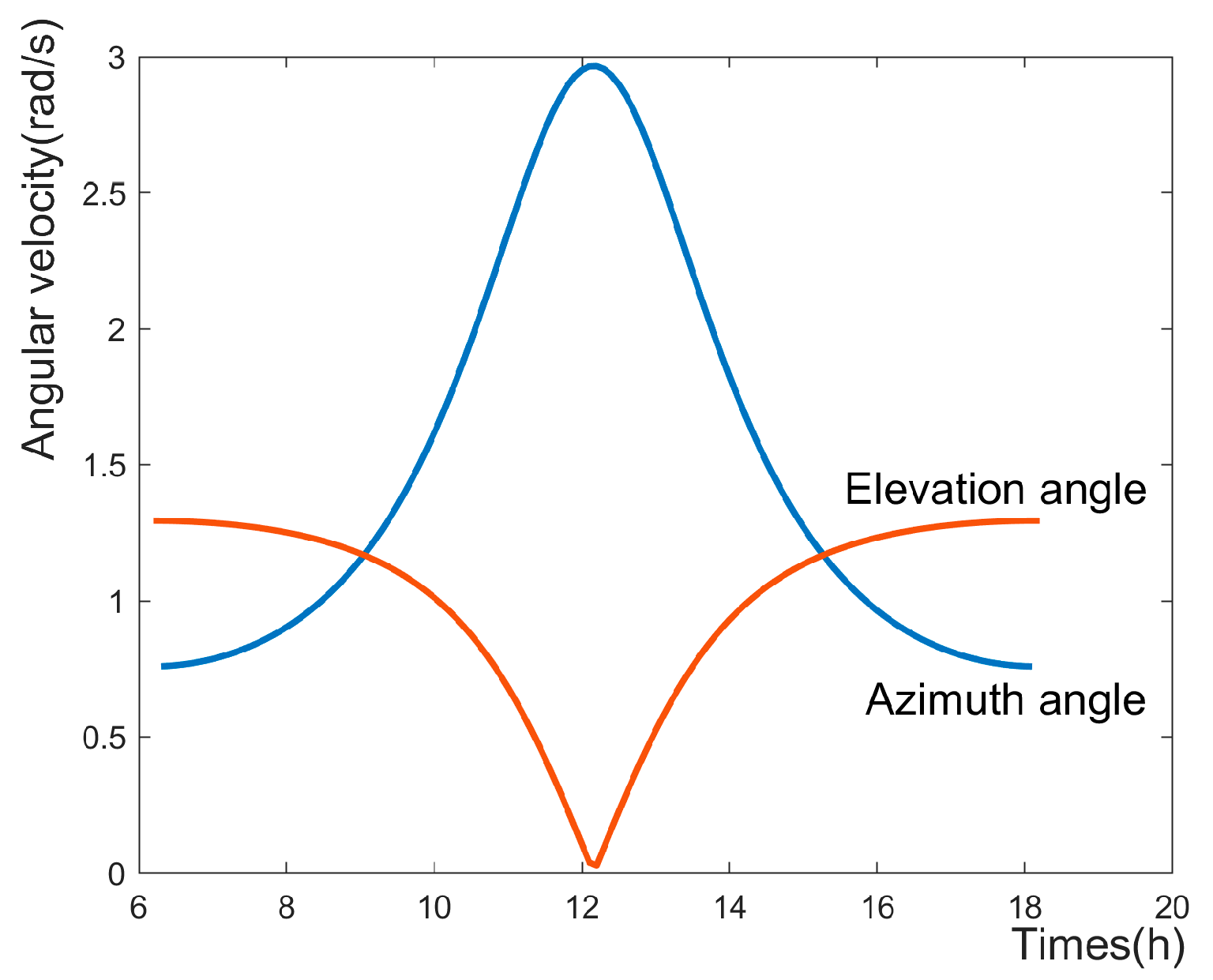
The angular speeds of the Sun’s azimuth and elevation angles are different throughout the day, so in order to avoid the cams alternating between accelerating and decelerating repeatedly during operation, resulting in a self-locking situation where the pressure angle is too large, the cams are made to perform only accelerating or decelerating motions during operation.

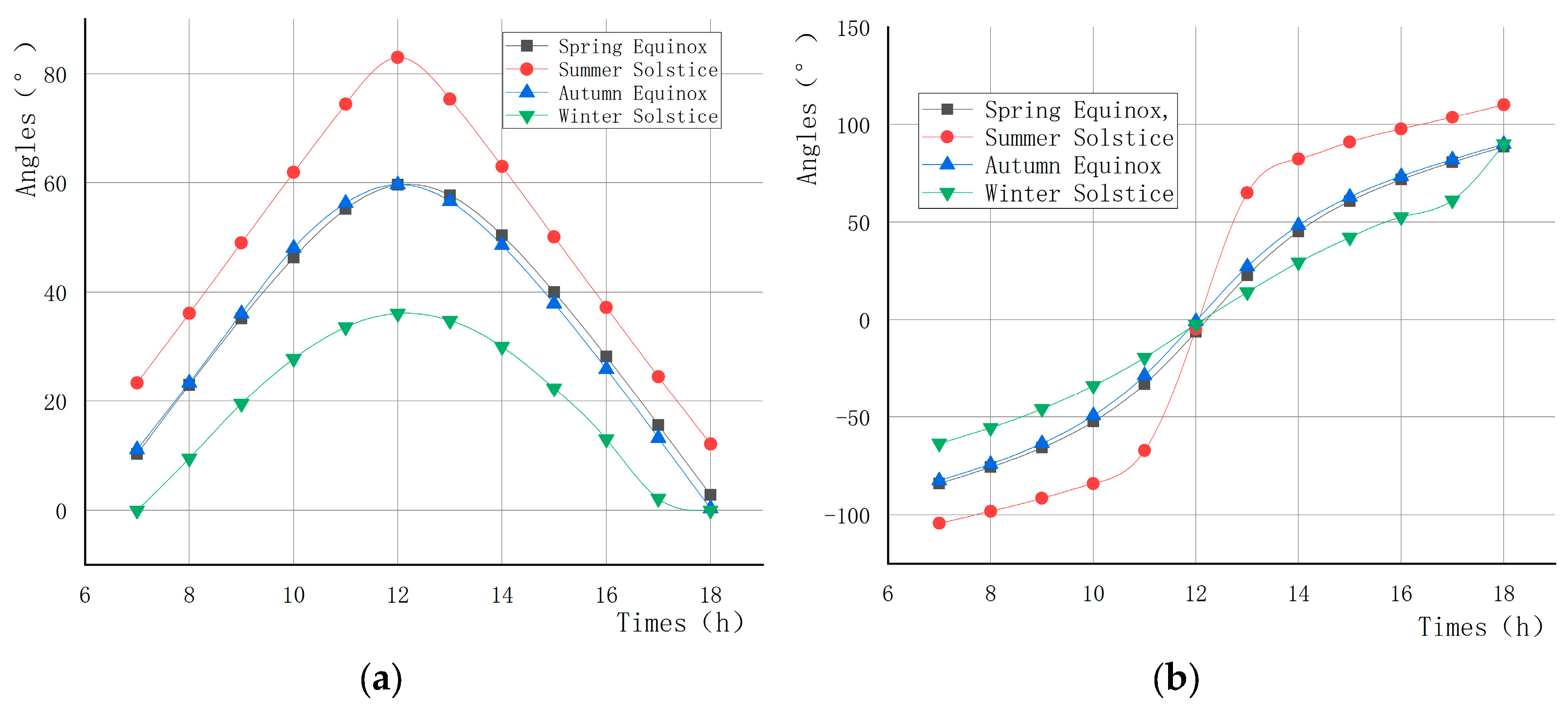
As shown in Figure 7, MATLAB software is used to calculate and plot the variation curves of the angular velocity ${\omega }_{\gamma }$ of the solar azimuth and the angular velocity ${\omega }_{\alpha }$ of the elevation angle, respectively. The moment when the azimuth angular velocity ${\omega }_{\gamma }$ and the elevation angular velocity ${\omega }_{\alpha }$ are equal for the first time is taken as the start time of the cam push period, and the moment when they are equal for the second time is taken as the end time of the cam push period, i.e., the cam is only accelerating or decelerating during the push period, which avoids the self-locking phenomenon of the cam having too large a pressure angle during the push period.

The cam pressure angle is the high vice contact point of the positive pressure direction and of the cam follower force action point of the linear velocity direction of the acute angle, and the pressure angle of the expression of the cam used in this paper for the roller direct-acting follower plane rotary cam mechanism is [55]

$$\alpha =\arctan ({\displaystyle \frac{\frac{ds}{d\varphi }-\eta E}{S_b+S}})$$

(14)

where is $E$ eccentricity distance; $\eta$ is the sign coefficient of eccentricity distance, which is 1 for left offset and −1 for right offset, and the offset schematic is shown in Figure 8; ${\displaystyle \frac{ds}{d\varphi }}$ is the cam follower’s class speed; $S_b+S$ is the perpendicular distance between the center of the cam follower roller’s circle in the cam follower’s motion direction and the center of the cam’s rotation.

The contour curve equations of the cams are obtained based on the motion inversion using analytical geometry calculations, and the specific design process is as follows: According to a specific day of the Sun’s elevation angle of the movement trajectory of photovoltaic components of the angle change rule of the elevation axis, the use of spatial triangular geometric relationship to obtain the cam follower’s movement law, combined with the angular speed of the cam rotation change rule, can help to obtain the cam contour curve. Therefore, the cam structure of the four seasons can be replaced according to the change rule of the solar elevation angle in a year to improve the tracking accuracy of the photovoltaic bracket on the solar elevation angle.

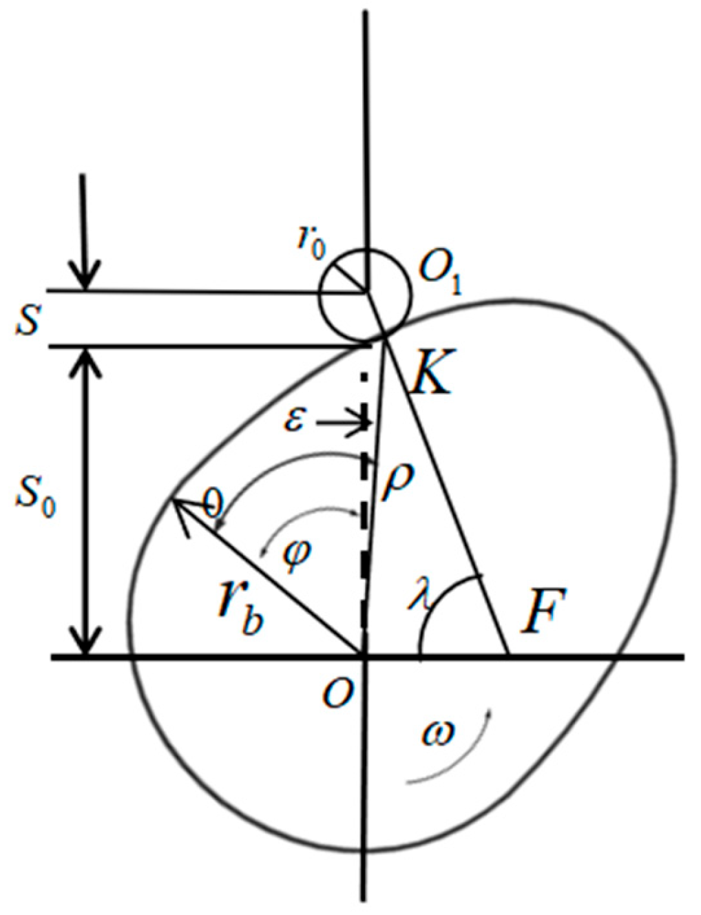
Based on the solar azimuth and elevation angles and the local latitude, the theoretical profile equation of the cam is obtained using the following analytical method:

$$\left\{\begin{array}{l}\rho =\sqrt{{({\displaystyle \frac{ds}{d\varphi }})}^2+{(\sqrt{\Delta S^2+{({\displaystyle \frac{ds}{d\varphi }})}^2}-r_0{}^2)}^2-2{\displaystyle \frac{ds}{d\varphi }}\cdot (\sqrt{\Delta S^2+{({\displaystyle \frac{ds}{d\varphi }})}^2-r_0})\cdot \cos \lambda }\\ \theta =\varphi +\epsilon \end{array}\right.$$

(15)

where ${\displaystyle \frac{ds}{d\varphi }}$ is the class speed of the cam follower, $\Delta S$ is the length of $AO$ minus the length of the cam follower, $r_0$ is the radius of the roller, $\lambda$ is the angle between the line connecting the center of the roller and the point of contact of the cam surface and the horizontal, $\varphi$ is the angle of rotation of the cam, and $\epsilon$ is the angle between the line connecting the center of the roller and the center of rotation of the cam and the line connecting the point of contact of the cam surface and the center of rotation of the cam, and the specific positions and sizes of the individual parameters are expressed as shown in Figure 9 [56].

The formulae for each parameter are as follows:

$${\displaystyle \frac{ds}{d\varphi }}={\displaystyle \frac{{\omega }_{\alpha }\cdot l_{AB}}{{\omega }_{\gamma }\cdot {\cos }^2\alpha }}$$

(16)

$$\lambda =\arctan ({\displaystyle \frac{\Delta S}{ds/d\varphi }})$$

(17)

$$\Delta S=l_{AO}-l_{cam\begin{array}{}\end{array}follower}$$

(18)

$$\epsilon =\arcsin ({\displaystyle \frac{r_0\cdot \cos \lambda }{\rho }})$$

(19)

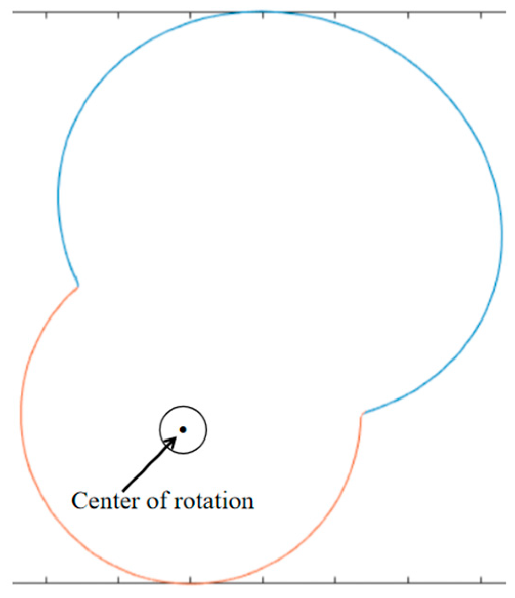
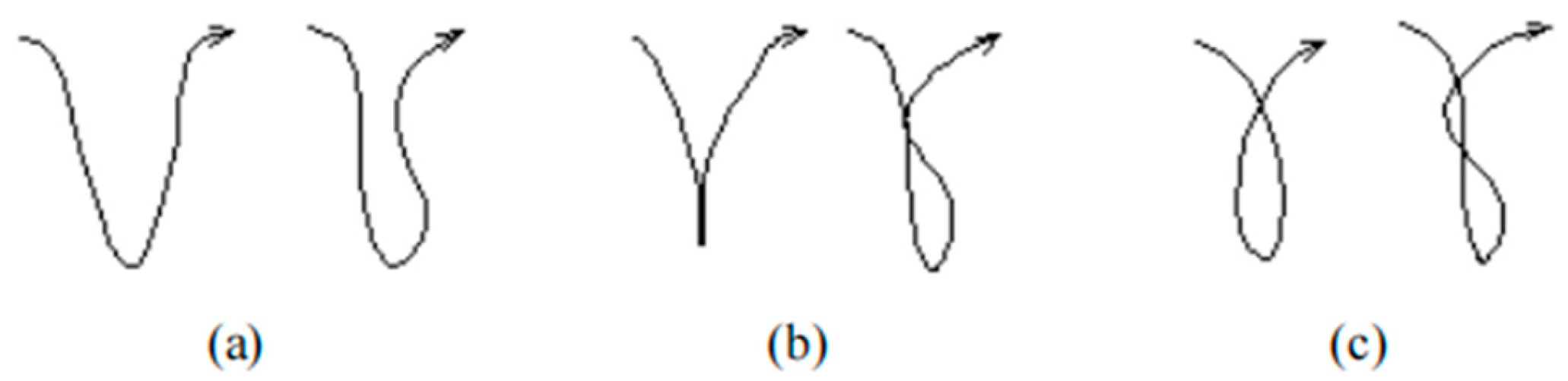
Taking place in Wuhan City as an example, which is located at 114°35′ E longitude and 30°38′ N latitude, the contour curve of the cam is calculated and plotted according to Equations (15)–(19), as shown in Figure 10, and it is found that the cam contour line has an obvious concave portion in the near-rest period at the junction of the push period and the return period. As shown in Figure 11, when the cam roller passes through the lower concave part of the cam surface, the running trajectory of the roller center may appear as (a) phase separation, (b) tangent, (c) intersection of three types; if the cam follower roller parameters are not selected reasonably, the running trajectory of the cam follower roller will appear in the intersection phenomenon, as shown in Figure 11c. At this time, the pressure angle of the cam mechanism changes dramatically, resulting in the cam mechanism self-locking. This paper refers to this phenomenon as the cam mechanism of the top cut phenomenon [57].

When the cam follower is a pointed follower, i.e., when the cam follower’s roller radius is 0, the cam follower passes through the concave portion of the cam surface with the roller center generating a running track, as shown in Figure 11a, and at this time, there is no top-cutting in the cam mechanism. When the cam follower stands for the roller follower, with the gradual increase in the cam follower roller radius, the cam surface in and out of the concave part of the two parts of the roller center of the running track will gradually close. When the cam follower roller radius increases to a certain extent, the roller center will produce the running track shown in Figure 11b, and reach the critical point of the cam self-locking. If the radius of the cam follower roller is larger than the critical value, it will produce a running trajectory as shown in Figure 11c, at which time the pressure angle of the cam mechanism increases sharply and the cam mechanism undergoes top-cutting.

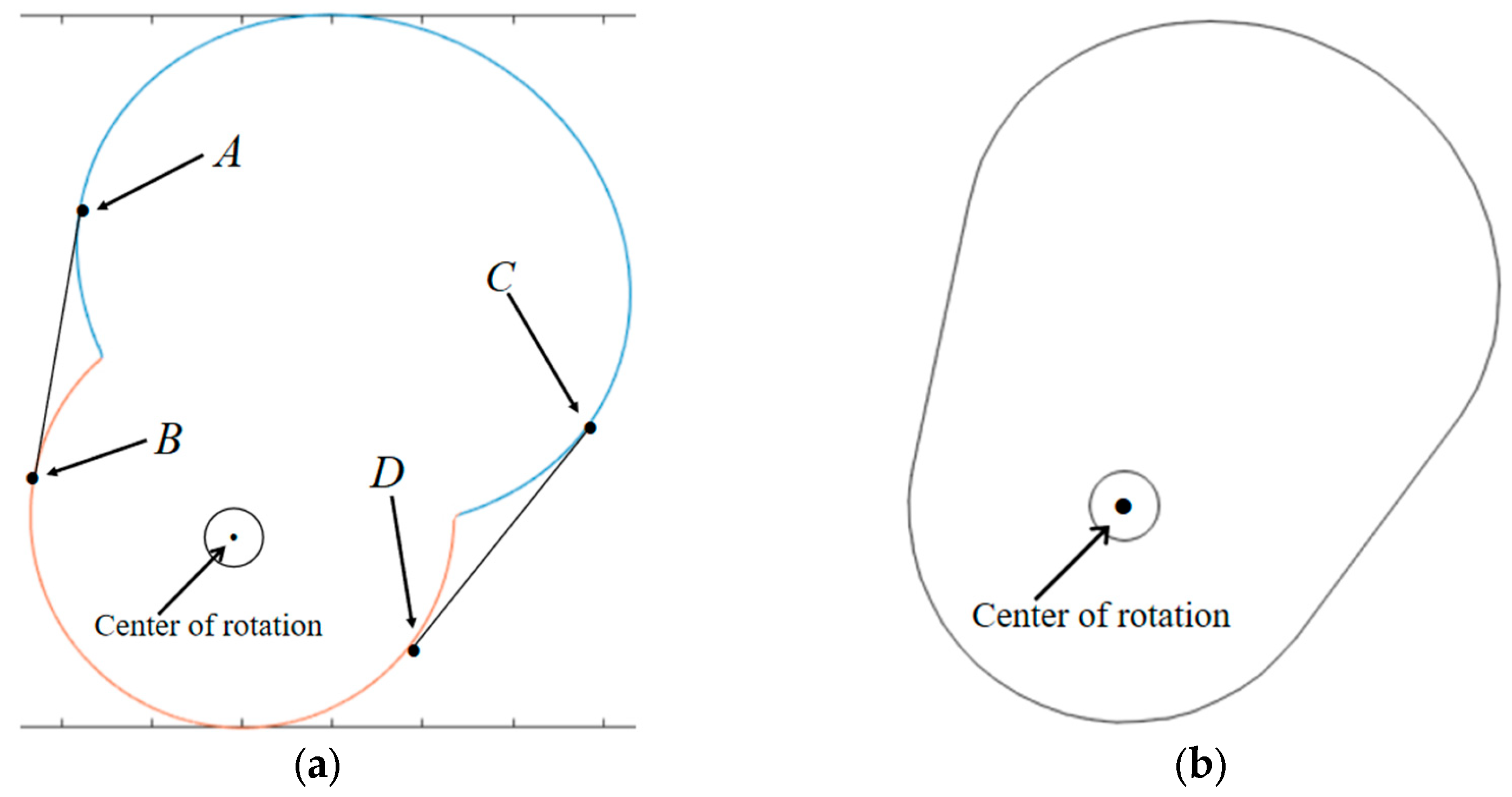
Due to the existence of corners in the theoretical cam profile curve, the cam follower is a roller direct-acting follower, which is affected by the diameter of the roller, and the cam needs to be engineered in order to avoid the phenomenon of hair top-cutting. As shown in Figure 12a, according to the characteristics of the cam contour curve in the near-rest period and the push period, corresponding to the two parts of the curve to find the tangent line slope of the same point, that is, $K_A=K_B$, $K_C=K_D$, will be used to correct the angle of the convex contour line of the two–two connection, and the corrected cam contour curve is shown in Figure 12b. The correction of both convex contour lines makes the cam mechanism smooth and flat during the working process and avoids the phenomenon of top-cutting, which causes the pressure angle to change and thus affects the normal working condition.

At this time, the tracking accuracy of the tracking bracket on the Sun’s elevation angle will be reduced, but due to the two corresponding specific times for the morning sunrise as well as evening sunset, the Sun’s light intensity is not high at this time. Even if this time is completely tracked, the additional power generation gain generated by the PV module is also minimal, so in practice, the loss of power generation generated during this time period is negligible.

4. Adaptability Analysis of Quasi-Biaxial Tracker

In order to illustrate the adaptability of the quasi-biaxial tracking system to different conditions, this chapter analyzes the position of the Sun at different latitude and longitude regions and during different seasons, as well as explains how the quasi-biaxial tracking system adapts to the different conditions.

4.1. Adaptation to Different Latitudes

Considering the differences in the solar position in different regions, the solar position trajectories in different regions at the same time are compared and analyzed, and the azimuth and elevation angles of the Sun in different regions are calculated according to Equations (1) and (2). As shown in Figure 13, the MATLAB (2021b) software is used to calculate and plot the solar position changes in the Wuhan area with the Shanghai area and Shenzhen area, where the latitude of the Wuhan and Shanghai areas is the same and the longitude is different; the longitude of the Wuhan and Shenzhen areas is the same and the latitude is different.

According to the comparison of solar azimuth and elevation angles in different regions in Figure 13, it can be seen that the changes in solar azimuth angle in different latitude regions in one day are exactly the same, but the changes in solar elevation angle have different trajectories; the solar azimuth angle in different longitude regions is the same, and the changes in elevation angle are also the same, and the changes in azimuth and elevation angle in Shanghai are advanced in overall time due to the time difference.

Therefore, in order to adapt to the differences in solar position in different regions, it is necessary to change the corresponding parameters in the quasi-biaxial tracking system. For regions with the same latitude, it is only necessary to change the start and end tracking time of the control system, and there is no need to change the parameters of the cam mechanism in order to adapt to the changes in the Sun’s position; for regions with different latitudes, the Sun’s azimuthal trajectory is the same, and there is no need to change the tracking strategy of the control system; for the differences in the elevation angle, it is necessary to change the parameters of the cam mechanism in order to adapt to the changes in the Sun’s elevation angle at different latitudes.

4.2. Adaptation to Different Seasons

Taking the area where Wuhan Textile University is located as an example, the changes in solar elevation angle and azimuth angle for four special days of Spring equinox, Summer solstice, Autumn equinox, and Winter solstice in the year 2024 are calculated based on Equations (1) and (2), which are shown in the following Figure 14:

From Figure 14, it can be seen that the Sun’s elevation angle takes the shape of a parabola and reaches its maximum at 12 noon. The Sun’s elevation angle is at its maximum on the Summer Solstice and at its minimum on the Winter Solstice, and the magnitude of the Sun’s elevation angle varies between the Winter Solstice and Summer Solstice over the course of the year. The azimuth angle takes the shape of a cubic function curve, changing slowly at sunrise and sunset and more rapidly at noon.

Since the azimuth angle is tracked by the motor directly driving the photovoltaic module, it is only necessary to change the calculation parameters of the azimuth position of the Sun in the control system to correctly calculate the azimuth angle of the Sun and drive the photovoltaic module to track it accurately. Since the mechanical device has the disadvantage of output uniqueness, for the change in the Sun’s elevation angle in the four seasons of the year, the cam mechanism with different parameters can be replaced according to the change rule of the Sun’s azimuth and elevation angle in a specific period of the year, in order to improve the tracking accuracy of the photovoltaic bracket for the Sun’s elevation angle.

5. Simulation and Analysis

Taking the area where Wuhan Textile University is located, which is located at 114°35′ E longitude and 30°38′ N latitude, as an example, the performance of different types of brackets was analyzed and compared indirectly by simulating and modeling the solar irradiance received by PV modules applying different bracket types.

5.1. Design of Simulation Conditions

Simulation 1: Select a representative date in a year of the Sun’s change law as the simulation of the solar motion model. The simulation of the selected date of 22 September 2024, according to Equations (1) and (2), is performed to obtain the day of the Sun’s elevation angle and azimuth angle of the movement trajectory, and MATLAB software is used to draw the obtained sun azimuth angle and elevation angle of the change curve, as shown in Figure 15. The intensity of solar radiation received by PV modules with three types of brackets applied on that day is simulated and analyzed according to the law of motion of the Sun on that day. Where the two drive motors of the dual-axis tracking bracket are tracked according to the azimuthal curve and the elevation angle curve, the drive motor of the quasi-biaxial solar tracker designed in this paper is tracked according to the azimuthal curve. The day is located in the Autumn Equinox of the local time, at which time the optimal inclination angle of the fixed bracket is 40°, so the optimal inclination of the fixed bracket on that day is fixed to the due south direction with an inclination angle of 40°. PVsyst (7.4) software was used to simulate the variation in solar irradiation intensity received by the PV modules applying the three types of brackets during the day, and the results obtained were compared and analyzed.

Simulation 2: The elevation angle of the Sun changes every day in a year, but the elevation angle tracking mechanism of the bracket designed in this paper has only one kind of motion law without changing the cam mechanism. Considering the influence of the change in the Sun’s elevation angle on the performance of the bracket in all the seasons, this simulation sets the simulation period as a one-year time, and the date is from 1 January 2024 to 31 December 2024. Analyze and compare the solar irradiance received by PV modules applying dual-axis tracking brackets, quasi-biaxial tracking brackets, and optimal inclination fixed brackets. The dual-axis tracking bracket tracks accurately according to the daily Sun movement pattern; the drive motor of the quasi-biaxial tracking bracket is tracked according to the daily Sun azimuth change. Since this simulation does not replace the cam mechanism of the quasi-biaxial tracking bracket in one year, and its elevation angle tracking mechanism can only track one kind of solar elevation change law, the inclination angle of the fixed bracket is likewise not adjusted in one year. According to the change rule of the solar elevation angle of the simulation site in a year, the inclination angle of the optimal inclination fixed bracket in a year is calculated to be 33°, so the optimal inclination fixed bracket in the simulation is fixed in the south direction, and the inclination angle is 33°. Thanks to the use of the same PVsyst software on the application of the dual-axis tracking bracket, quasi-biaxial tracking bracket, and the annual optimal inclination angle of the fixed bracket of the PV module subjected to solar irradiance simulation experiments, the simulation results obtained make it possible to analyze and further validate the effectiveness of the bracket design.

5.2. Simulation Results Analysis

Simulation Result 1: Taking the variation curve of the Sun in Figure 15 as the law of motion of the tracking program, the solar irradiance received by the PV modules applying the three types of brackets is analyzed and compared using the PVsyst software, and the simulation results are shown in Figure 16. The three curves in the figure show the variation curves of solar irradiance to which the PV modules are subjected with the application of a dual-axis tracking bracket, a quasi-biaxial solar tracker designed in this paper, and an optimal inclination fixed bracket. The comparison of the simulation results shows that the solar irradiance of the PV modules applying the type of bracket designed in this paper is slightly lower than that of the dual-axis tracking bracket and significantly higher than that of the optimal inclination fixed bracket, which indirectly indicates that the performance of the quasi-biaxial solar tracker designed in this paper is higher than that of the optimal inclination fixed bracket and slightly lower than that of the dual-axis tracking bracket with two drive motors.

Simulation Results 2: The solar irradiance per moment on the unit square meter of the PV module is obtained by simulating the solar irradiance received by the PV modules applying a dual-axis tracking bracket, quasi-biaxial tracking bracket, and annual optimal inclination fixed bracket in one year. The daily solar irradiance is integrated to obtain the total value of the energy of solar irradiance received by the PV module in a day, which in turn gives the total value of the energy of solar irradiance received per unit area of the PV module in each month, as shown in

Table 1. Total value of solar radiation energy received by PV modules per month.

Months	Dual-Axis Tracking Bracket (Wh/m2)	Quasi-Biaxial Solar Tracker (Wh/m2)	Fixed Bracket with 33° Inclination (Wh/m2)
1	94,527	86,623.1	78,772.5
2	82,191.6	72,866.5	68,493
3	131,161.6	121,467.4	111,153.9
4	142,763	134,451.8	120,985.6
5	155,174.5	145,086.2	12,9312.1
6	137,725.5	134,904.5	119,761.3
7	173,038.7	169,036.8	147,896.3
8	170,100.9	166,635.7	145,385.4
9	154,308.1	147,920.5	130,769.6
10	132,696.3	123,623.4	112,454.5
11	108,585.7	100,583.5	91,248.5
12	92,882.2	84,884.2	77,401.8

. Figure 17 shows the variation curves of the total monthly irradiance value of the PV modules applying the three types of brackets. Overall, since the dual-axis tracking bracket can accurately track the position of the Sun at all times, and the quasi-biaxial tracking bracket can adjust the orientation of the PV module with the change in the Sun’s position, the monthly receipts of the solar irradiance per unit area of the PV module applying the dual-axis tracking bracket are higher than those of the PV module applying the quasi-biaxial tracking bracket and the annual optimal inclination fixed bracket. Also, the monthly reception of solar irradiance of PV modules applying a quasi-biaxial tracking bracket is higher than that of PV modules applying an annual optimal inclination fixed bracket and slightly lower than that of PV modules applying a dual-axis tracking bracket. Similarly indirectly, the quasi-biaxial tracking bracket was demonstrated to have higher performance than the optimal inclination fixed bracket and slightly lower than the dual-axis tracking bracket.

The results of Simulation 1 and Simulation 2 reveal that the solar irradiation intensity received by the surface of the PV module applying the quasi-biaxial tracking bracket is significantly higher than that of the PV module applying the optimal inclination fixed bracket. This difference indicates that the PV system with the application of a quasi-biaxial tracking bracket is able to obtain more total solar irradiation under the same operating time and environmental conditions. Since the output capacity of a PV module is positively related to the amount of solar irradiation it receives, and increasing the amount of solar radiation captured can be converted into more power generation, total irradiation can be used to assess the ability of a PV module to generate power. Therefore, a PV system applying a quasi-biaxial tracking bracket generates more electricity than an optimally inclined fixed system with the same conversion efficiency as the PV module.

The effectiveness of the bracket design was verified through one-day and one-year simulation experiments conducted in the area where Wuhan Textile University is located. The bracket can effectively increase the solar irradiance received by the PV modules not only on the day of the design day but also every day of the year, thus improving the overall system power generation efficiency.

6. Economic Analysis of Quasi-Biaxial Tracker Systems

In this part, the LCOE economic analysis of the quasi-biaxial tracking system is carried out in the region of Wuhan Textile University as an example, and an economic comparative study is conducted with the dual-axis tracking system.

6.1. Calculation of Electricity Generation from Photovoltaic Systems

The amount of electricity generated by PV modules in a PV system based on the solar radiation received by the PV modules is calculated by the following formula:

$$EP={\displaystyle {\int }_{t_0}^{t_1}{\eta }_{ps}\cdot A\cdot G_s\left(t\right)dt}$$

(20)

where EP is the electricity generation of the PV module; ${\eta }_{ps}$ is the conversion efficiency of the PV module; $A$ is the area of the PV module; $G_S$ is the light irradiance in the standard state; $t_0$, $t_1$ are the time when the PV module receives the beginning and the end of the solar radiation.

Assuming that the conversion efficiency of the PV module ${\eta }_{ps}$ is 100% and the area $A$ of the PV module is 1 m², the amount of electricity generated by the PV module is $EP={\displaystyle {\int }_{t_0}^{t_1}{G}_S\left(t\right)}dt$, which is numerically equal to the total value of solar radiation energy received by the PV module.

Taking the area where Wuhan Textile University is located as an example, the power generation of PV modules is calculated based on the solar radiation received by PV modules of the dual-axis tracking system and quasi-biaxial tracking system in Figure 15, and the specific values are shown in

Table 2. Electricity generation from different racking systems.

Photovoltaic System Types	Electricity Generation (kWh)
Dual-axis tracking system	1575.2
Quasi-Biaxial Tracking System	1488.1

.

6.2. Economic Analysis of PV Systems

LCOE is a widely used metric for evaluating the economic feasibility of PV systems. LCOE is the discounted ratio of all costs incurred by a PV electricity generation project over its entire life cycle to the entire amount of grid-ready electricity and is equal to the ratio of the sum of the costs incurred over the life cycle of the project to the present value of the total amount of electricity generated by the equipment over its life-cycle service. The formula for calculating LCOE is as follows:

$$LCOE={\displaystyle \frac{C_0+{\displaystyle {\sum }_{t=1}^T\frac{C_t\cdot {\left(1+i\right)}^t}{{\left(1+j\right)}^t}}}{{\displaystyle {\sum }_{t=1}^T\frac{E_t\cdot {\left(1-d\right)}^t}{{\left(1+j\right)}^t}}}}$$

(21)

In Equation (21), $C_0$ is the initial capital expenditure of the project, $T$ is the projected life of the project or the contract time, $t$ is the operating life of the system, $C_t$ is the cost of the project at time “$t$”, $i$ is the inflation rate, $d$ is the degradation rate of the PV modules, $j$ is the discount rate, and $E_t$ is the amount of energy produced at time “$t$”.

The LCOE of a PV power project mainly includes construction investment costs and operation and maintenance costs, of which the initial investment costs include PV cells, mounting brackets, wires, inverters, and land rental funds. As shown in

Table 3. LCOE cost components for PV electricity generation systems.

	Investment Projects	Unit (of Measure)	Reference Value
Initial investment	Photovoltaic Module	yuan/W	1.82
	Quasi-Biaxial Tracking Bracket Equipment	yuan/W	2
	Dual-axis tracking bracket Equipment	yuan/W	4.8
	Monitoring Systems	yuan/W	0.15
	Survey, design, equipment installation, and site fees	yuan/W	1.1
	Inverter	yuan/W	0.545
	Land rental costs	yuan/W	0.05
Maintenance costs	Maintenance costs of equipment and materials	yuan/W	Acquisition cost * 0.3%
	Cleaning labor costs	yuan/W	0.02
	Labor wage	yuan	55,000
Additional information	Discount rate	%	5
	Project Life Cycle	annum	25
	Inflation rate	%	7.4
	Annual degradation rate of photovoltaic cells	%	0.5

, the initial investment and maintenance cost information can be obtained based on the existing information and the calculation of the relevant parameters of the study site.

In this paper, a 1 MW PV system is installed in the Wuhan area as an example, located at 30°38′ N latitude and 114°35′ E longitude. In order to reduce the maintenance cost of the system, the quasi-biaxial tracking system uses a cam mechanism in one year. Based on the cost data in Table 3, the total cost of the quasi-biaxial tracking PV system and the dual-axis tracking PV system is calculated, and the LCOEs under different bracket types of the PV system are calculated by combining the power generation of each of the two PV systems, and the specific results are shown in

Table 4. LCOE and related parameters of different stent systems.

Projects	Quasi-Biaxial Tracker	Dual-Axis Tracker
First year’s electricity generation (MWh)	1488.1	1575.2
Total life cycle cost (ten thousand yuan)	992.2	1333.8
Cost of investment (ten thousand yuan)	561.5	846.5
LCOE (yuan/kWh)	0.4415	0.5935

. The LCOE of the quasi-biaxial tracking system is 0.4415 Yuan/kWh, and that of the biaxial tracking system is 0.5835 Yuan/kWh. The main reason for this difference is that the initial investment cost of the dual-axis tracking system is 50.75% higher than that of the quasi-biaxial tracking system, and the total power generation is only 5.85% higher.

The above analysis shows that, in Wuhan, the LCOE of the PV system with the quasi-biaxial tracking bracket is lower than that of the dual-axis tracking bracket, which indicates that the quasi-biaxial tracking system has lower power generation cost and better economic competitiveness compared to the dual-axis tracking system.

7. Experimental Validation

In order to further verify the feasibility of this design, the required components are designed and machined, and a small experimental verification platform is constructed to verify the performance of the quasi-biaxial solar tracker designed in this paper.

7.1. Experimental Design

Wuhan Textile University is the region selected as an example, with 22 September 2024, as the design date. The change law of the Sun’s elevation angle on that day and the average value of the Sun’s elevation angle change in a year are closest to the Sun’s movement trajectory on that day, which serves as the basis for obtaining the specific parameters of the parts, after the engineering design, manufacturing, and processing of the relevant parts of the bracket designed in this paper.

In order to simulate the role of the quasi-biaxial tracking system in enhancing the power generation efficiency in a real working environment, two different types of weather, representative of sunny and cloudy days, are selected for the comparative test of the power generation efficiency of the two systems, in which 22 September 2024, is selected as the experimental data for sunny days, and 30 September 2024, is selected as the experimental data for cloudy days. The output power of the PV modules in the two types of weather is compared and analyzed, thus verifying the role of the quasi-biaxial tracking system in enhancing the power generation efficiency.

Figure 18 shows the experimental test site, which can be compared with the best inclination fixed bracket to analyze the output power of its PV modules. For the optimal inclination fixed bracket tilt angle of 40°, fixed for the due south direction, the quasi-biaxial tracking bracket designed in this paper is used at this time for the initial position of the Sun before the Sun rises. ARDUINO is used to control the drive motor and to change the speed of rotation once every six minutes, and to achieve the tracking of photovoltaic modules to the solar azimuth, the specific angle of rotation and speed of the day and the Sun’s azimuth change in line within the same day.

Figure 19 shows the output PV line of the PV module, located on the backside of the PV panel. The peak power of the PV module is 25 W, the open-circuit voltage is 21.67 V, and the short-circuit current is 1.67 A. The open-circuit voltage and short-circuit current of the PV module are measured and recorded every hour, and the output power of the PV module is calculated as the product of the measured voltage and current.

7.2. Analysis of the Experimental Result

Analysis of experimental results under sunny weather: The experimental test results are shown in

Table 5. Measured open-circuit voltage and short-circuit current of a photovoltaic module on a sunny day.

Times (h)	Quasi-Biaxial Solar Tracker		Fixed Bracket with 40° Inclination
	Voltage (V)	Current (A)	Voltage (V)	Current (A)
6	19.2	0	19.2	0
7	19.9	0.16	19.9	0.03
8	21.7	0.4	21.7	0.14
9	22.2	0.64	21.9	0.35
10	23.1	0.95	22.9	0.61
11	22.9	1.13	22.6	0.88
12	22.5	1.22	22.6	1.24
13	22.8	1.22	22.4	1.23
14	22.8	1.17	22.4	0.7
15	22.2	0.96	22.0	0.36
16	22.0	0.6	21.8	0.2
17	21.9	0.33	21.7	0.1
18	20.6	0.15	20.2	0.04
19	19.5	0	19.3	0

. Applying the quasi-biaxial solar tracker designed in this paper with the optimal inclination fixed bracket of the PV module, the open-circuit voltage is almost the same, the short-circuit current of the PV module is greater than that of the optimal inclination fixed bracket in the morning and afternoon, and the short-circuit currents of the two are almost equal in the middle of the day when the light intensity is greater. The output power of the two PV modules obtained from the calculation is shown in Figure 20. Comparing the output power of the two bracket types, it can be seen that the output power of the PV module with the optimal inclination fixed bracket is lower, and the total output power of the PV module with the application of the quasi-biaxial solar tracker is much larger than that of the PV module with the optimal inclination fixed bracket during the working cycle, so it can be seen that the PV module with the application of the bracket designed in this paper produces more electricity under the same working environment. The PV modules with the bracket type designed in this paper generate more power in the same working cycle.

Analysis of experimental results under cloudy weather: The experimental test results are shown in

Table 6. Measured open-circuit voltage and short-circuit current of photovoltaic components on cloudy days.

Times (h)	Quasi-Biaxial Solar Tracker		Fixed Bracket with 40° Inclination
	Voltage (V)	Current (A)	Voltage (V)	Current (A)
6	19	0	19.1	0
7	19.5	0.03	19.9	0.02
8	21.5	0.03	21.7	0.01
9	21.9	0.04	21.7	0.02
10	22.1	0.06	22.5	0.04
11	22.7	0.06	22.3	0.07
12	22.5	0.08	22.3	0.08
13	22.6	0.06	22	0.06
14	22.1	0.05	21.9	0.05
15	22.2	0.04	21.8	0.04
16	21.9	0.04	21.6	0.03
17	21.7	0.01	21.5	0.01
18	19.2	0	19.2	0
19	19	0	19.1	0

. The open-circuit voltage and short-circuit current of the PV modules, applying the quasi-biaxial tracking bracket designed in this paper, the optimal inclination fixed brackets are almost equal. By calculating the output power changes of the two PV modules, as shown in Figure 21, it can be seen that, in cloudy and rainy weather, the intensity of the Sun’s rays is very weak, the output power of the PV module is very low, and the application of quasi-biaxial tracking bracket PV modules and the total output power of the optimal inclination of the PV modules of the fixed-angle bracket is almost the same. It can be seen that the PV modules applying the type of mounts designed in this paper have almost no difference with the fixed bracket under the rainy weather working environment, so the tracking of the Sun position by the quasi-biaxial tracking system can be suspended to reduce the operating cost during rainy weather.

Through the experimental analysis of the two types of photovoltaic systems in different weathers, it can be seen that the quasi-biaxial tracking bracket can obviously improve the output power of the photovoltaic modules in sunny weather, when the precise tracking of the Sun’s position can be enough to improve the power generation of the photovoltaic system better. However, in cloudy and rainy weather, due to the weak intensity of the Sun’s light, the output power of the PV modules in both the tracking system and the fixed system is very low. So in cloudy and rainy weather, the tracking system can be suspended to track the Sun in order to reduce the cost of the tracking system.

8. Discussion

In order to better balance the relationship between the power generation efficiency of the PV system and the system cost, this paper presents a systematic design of a single motor-driven dual-axis solar tracking bracket, with an azimuth angle tracking mechanism and an elevation angle tracking mechanism based on the Sun’s motion law. A mechanical transmission containing a bevel gear mechanism and a cam mechanism is used to replace the motor driving the elevation axis, and the tracking of the PV module to the Sun in two directions is achieved by minimizing the number of motors. At the same time, the cam mechanism can be replaced to change the shape of the cam’s contour to enable the PV module’s elevation axis to track at different angles, so that the bracket can be adapted to all days of the year. The bracket adds an azimuth tracking mechanism to the azimuth single-axis tracking bracket, which increases the tracking accuracy of the Sun to a certain extent. Although the tracking accuracy of the elevation axis of this bracket is lower than that of the dual-axis tracking bracket, the reduction in the number of drive motors for the expensive parts has resulted in a relative reduction in the cost of construction as well as the cost of maintenance at a later stage. This ultimately improves the economic efficiency of the PV power generation system during the production cycle. The feasibility of the bracket design is finally verified by simulation and physical experiment, which provides a reference value for the design and research of PV tracking brackets. However, due to the mechanical device having a certain hard drive relationship, the output power of the designed bracket has the disadvantages of uniqueness, the structure of the same cam can not adapt to the change in the Sun’s elevation angle across the latitude region and the four seasons of the year, and it cannot reach the tracking accuracy of the dual-axis tracking bracket with two drive motors outside a specific date, so in the future research can be continued in-depth from this perspective to truly realize the accurate tracking of the Sun by photovoltaic modules.

9. Conclusions

• By replacing the drive motor that drives the elevation axis with a mechanical transmission that includes a bevel gear mechanism and a cam mechanism, the tracking of the Sun by the PV module in both directions is achieved with a minimized number of motors.
• Changing the profile shape of the cams by replacing the cam mechanism enables the PV module elevation axis to track different angle changes, so the bracket can be adapted to all days of the year.
• Although the tracking accuracy of the elevation axis of this mount is lower than that of the dual-axis tracking bracket, the reduction in the number of drive motors for the expensive parts results in a relative reduction in the cost of construction as well as the cost of maintenance in the later stages, which ultimately improves the economic efficiency of the photovoltaic power generation system during the production cycle.
• The feasibility of the bracket design is verified by simulation and physical experiment, which provides a reference value for the design and research of PV tracking brackets.

References

1. Zhang, G.; Zeng, G.; Li, C.; Yang, X. Impact of PDO and AMO on interdecadal variability in extreme high temperatures in North China over the most recent 40-year period. Clim. Dyn. 2020, 54, 3003–3020. [Google Scholar] [CrossRef]
2. King, A.; Karoly, D.; Henley, B. Australian climate extremes at 1.5 °C and 2 °C of global warming. Nat. Clim. Chang. 2017, 7, 412–416. [Google Scholar] [CrossRef]
3. Jacobs, K.L.; Buizer, J.L.; Moser, S.C. The third US national climate assessment: Innovations in science and engagement. Clim. Chang. 2016, 135, 1–7. [Google Scholar] [CrossRef]
4. Zhang, G.; Zeng, G.; Yang, X.; Jiang, Z. Future Changes in Extreme High Temperature over China at 1.5 °C–5 °C Global Warming Based on CMIP6 Simulations. Adv. Atmos. Sci. 2021, 38, 253–267. [Google Scholar] [CrossRef]
5. Racharla, S.; Rajan, K. Solar tracking system—A review. Int. J. Sustain. Eng. 2017, 10, 72–81. [Google Scholar] [CrossRef]
6. Yao, Y.; Hu, Y.; Gao, S.; Yang, G.; Du, J. A multipurpose dual-axis solar tracker with two tracking strategies. Renew. Energy 2014, 72, 88–98. [Google Scholar] [CrossRef]
7. Green, M.; Dunlop, E.; Hohl-Ebinger, J.; Yoshita, M.; Kopidakis, N.; Hao, X. Solar cell efficiency tables (version 57). Prog. Photovolt. Res. Appl. 2021, 29, 3–15. [Google Scholar] [CrossRef]
8. Mangherini, G.; Diolaiti, V.; Bernardoni, P.; Andreoli, A.; Vincenzi, D. Review of Façade Photovoltaic Solutions for Less Energy-Hungry Buildings. Energies 2023, 16, 6901. [Google Scholar] [CrossRef]
9. Mangherini, G.; Sollazzo, L.; Diolaiti, V.; Gawronska, M.; Sanna, C.; Damiano, A.; Vincenzi, D. Long-Term Reliability of Semi-Transparent Photovoltaic Panels Based on Luminescent Solar Concentrators. Energies 2025, 18, 674. [Google Scholar] [CrossRef]
10. Mangherini, G.; Baccega, E.; Diolaiti, V.; Vincenzi, D. Integration of Phase Change Material into PV Windows to Improve the Efficiency of Semi-Transparent Panels Based on Luminescent Solar Concentrator Technology. Sustainability 2024, 16, 11148. [Google Scholar] [CrossRef]
11. Mangherini, G.; Bernardoni, P.; Baccega, E.; Andreoli, A.; Diolaiti, V.; Vincenzi, D. Design of a Ventilated Façade Integrating a Luminescent Solar Concentrator Photovoltaic Panel. Sustainability 2023, 15, 9146. [Google Scholar] [CrossRef]
12. Bernardoni, P.; Mangherini, G.; Gjestila, M.; Andreoli, A.; Vincenzi, D. Performance Optimization of Luminescent Solar Concentrators under Several Shading Conditions. Energies 2021, 14, 816. [Google Scholar] [CrossRef]
13. Finster, C. El heliostato de la Universidad santa maria. Scientia 1962, 119, 5–20. [Google Scholar]
14. McFee, R.H. Power collection reduction by mirror surface non flatness and tracking error for a central receiver solar power system. Appl. Opt. 1975, 14, 1493–1502. [Google Scholar] [CrossRef]
15. Abdallah, S.; Nijmeh, S. Two axes sun tracking system with PLC control. Energy Convers. Manag. 2004, 45, 1931–1939. [Google Scholar] [CrossRef]
16. Song, J.; Zhu, Y.; Jin, Z.; Yang, Y. Daylighting system via fibers based on two-stage sun-tracking model. Sol. Energy 2014, 108, 331–339. [Google Scholar] [CrossRef]
17. Gabe, I.J.; Bühler, A.; Chesini, D.; Frosi, F. Design and implementation of a low-cost dual-axes autonomous solar tracker. In Proceedings of the 2017 IEEE 8th International Symposium on Power Electronics for Distributed Generation Systems (PEDG), Floria-nópolis, Brazil, 17–20 April 2017. [Google Scholar]
18. Yang, Z.; Xiao, Z. A Review of the Sustainable Development of Solar Photovoltaic Tracking System Technology. Energies 2023, 16, 7768. [Google Scholar] [CrossRef]
19. Tomson, T. Discrete two-positional tracking of solar collectors. Renew. Energy 2008, 33, 400–405. [Google Scholar] [CrossRef]
20. Huang, B.J.; Sun, F.S. Feasibility study of one axis three positions tracking solar PV with low concentration ratio reflector. Energy Convers. Manag. 2007, 48, 1273–1280. [Google Scholar] [CrossRef]
21. Bentaher, H.; Kaich, H.; Ayadi, N.; Hmouda, M.B.; Maalej, A.; Lemmer, U. A simple tracking system to monitor solar PV panels. Energy Convers. Manag. 2014, 78, 872–875. [Google Scholar] [CrossRef]
22. Skouri, S.; Ali, A.B.; Bouadila, S.; Salah, M.B.; Nasrallah, S.B. Design and construction of sun tracking systems for solar parabolic concentrator displacement. Renew. Sustain. Energy Rev. 2016, 60, 1419–1429. [Google Scholar] [CrossRef]
23. Eldin, S.A.S.; Abd-Elhady, M.S.; Kandil, H.A. Feasibility of solar tracking systems for PV panels in hot and cold regions. Renew. Energy 2016, 85, 228–233. [Google Scholar] [CrossRef]
24. Poulek, V. Testing the new solar tracker with shape memory alloy actors. In Proceedings of the 1994 IEEE 1st World Conference on Photovoltaic Energy Conversion-WCPEC (A Joint Conference of PVSC, PVSEC and PSEC), Waikoloa, HI, USA, 5–9 December 1994; Volume 1. [Google Scholar] [CrossRef]
25. Sumathi, V.; Jayapragash, R.; Bakshi, A.; Akella, P.K. Solar tracking methods to maximize PV system output—A review of the methods adopted in recent decade. Renew. Sustain. Energy Rev. 2017, 74, 130–138. [Google Scholar] [CrossRef]
26. Ferdaus, R.A.; Mohammed, M.A.; Rahman, S.; Salehin, S.; Mannan, M.A. Energy efficient hybrid dual axis solar tracking system. J. Renew. Energy 2014, 2014, 629717. [Google Scholar] [CrossRef]
27. Singh, R.; Kumar, S.; Gehlot, A.; Pachauri, R. An imperative role of sun trackers in photovoltaic technology: A review. Renew. Sustain. Energy Rev. 2018, 82, 3263–3278. [Google Scholar] [CrossRef]
28. Zulkafli, R.S.; Bawazir, A.S.; Amin, N.A.M.; Hashim, M.S.M.; Majid, M.S.A.; Nasir, N.F.M. Dual axis solar tracking system in Perlis, Malaysia. J. Telecommun. Electron. Comput. Eng. 2018, 10, 91–94. [Google Scholar]
29. Neagoe, M.; Visa, I.; Burduhos, B.G.; Moldovan, M.D. Thermal load based adaptive tracking for flat plate solar collectors. Energy Procedia 2014, 48, 1401–1411. [Google Scholar] [CrossRef]
30. AL-Rousan, N.; Isa, N.A.M.; Desa, M.K.M. Correlation analysis and MLP/CMLP for optimum variables to predict orientation and tilt angles in intelligent solar tracking systems. Int. J. Energy Res. 2021, 45, 453–477. [Google Scholar] [CrossRef]
31. Mehdi, G.; Ali, N.; Hussain, S.; Zaidi, A.A.; Shah, A.H.; Azeem, M.M. Design and fabrication of automatic single axis solar tracker for solar panel. In Proceedings of the 2019 2nd International Conference on Computing, Mathematics and Engineering Technologies (iCoMET), Sukkur, Pakistan, 30–31 January 2019. [Google Scholar] [CrossRef]
32. Gutiérrez, S.; Rodrigo, P.M. Energetic analysis of simplified 2-position and 3-position North-South horizontal single-axis sun tracking concepts. Sol. Energy 2017, 157, 244–250. [Google Scholar] [CrossRef]
33. Dandu, S.C.R.; Sarla, A. Sun Tracking System. Bachelor’s Degree Thesis, Blekinge Institute of Technology, Karlskrona, Sweden, 2022. [Google Scholar]
34. Abdelghani-Idrissi, M.A.; Khalfallaoui, S.; Seguin, D.; Vernières-Hassimi, L.; Leveneur, S. Solar tracker for enhancement of the thermal efficiency of solar water heating system. Renew. Energy 2018, 119, 79–94. [Google Scholar] [CrossRef]
35. Jamroen, C.; Komkum, P.; Kohsri, S.; Himananto, W.; Panupintu, S.; Unkat, S. A low-cost dual-axis solar tracking system based on digital logic design: Design and implementation. Sustain. Energy Technol. Assess. 2020, 37, 100618. [Google Scholar] [CrossRef]
36. Hammoumi, A.E.; Motahhir, S.; Ghzizal, A.E.; Chalh, A.; Derouich, A. A simple and low-cost active dual-axis solar tracker. Energy Sci. Eng. 2018, 6, 607–620. [Google Scholar] [CrossRef]
37. Fahad, H.M.; Islam, A.; Islam, M.; Hasan, M.F.; Brishty, W.F.; Rahman, M.M. Comparative analysis of dual and single axis solar tracking system considering cloud cover. In Proceedings of the 2019 International Conference on Energy and Power Engineering (ICEPE), Dhaka, Bangladesh, 14–16 March 2019. [Google Scholar] [CrossRef]
38. Alexandru, C. Modelling and simulation of a single-motor bi-axial sun tracking mechanism. IOP Conf. Ser. Mater. Sci. Eng. 2022, 1256, 012021. [Google Scholar]
39. Ahmad, S.; Shafie, S.; Kadir, M.Z.A.A. Power feasibility of a low power consumption solar tracker. Procedia Environ. Sci. 2013, 17, 494–502. [Google Scholar] [CrossRef]
40. Zhang, P.; Zhou, G.; Zhu, Z.; Li, W.; Cai, Z. Numerical study on the properties of an active sun tracker for solar streetlight. Mechatronics 2013, 23, 1215–1222. [Google Scholar] [CrossRef]
41. Deb, G.; Roy, A.B. Use of solar tracking system for extracting solar energy. Int. J. Comput. Electr. Eng. 2012, 4, 42. [Google Scholar]
42. Şenpinar, A.; Cebeci, M. Evaluation of power output for fixed and two-axis tracking PVarrays. Appl. Energy 2012, 92, 677–685. [Google Scholar] [CrossRef]
43. Perpiñán, O. Cost of energy and mutual shadows in a two-axis tracking PV system. Renew. Energy 2012, 43, 331–342. [Google Scholar] [CrossRef]
44. Koussa, M.; Cheknane, A.; Hadji, S.M.H.S.N.; Haddadi, M.; Noureddine, S. Measured and modelled improvement in solar energy yield from flat plate photovoltaic systems utilizing different tracking systems and under a range of environmental conditions. Appl. Energy 2011, 88, 1756–1771. [Google Scholar] [CrossRef]
45. Abdollahpour, M.; Golzarian, M.R.; Rohani, A.; Zarchi, H.A. Development of a machine vision dual-axis solar tracking system. Sol. Energy 2018, 169, 136–143. [Google Scholar] [CrossRef]
46. Bazyari, S. A study on the effects of solar tracking systems on the performance of photovoltaic power plants. J. Power Energy Eng. 2014, 2, 718. [Google Scholar] [CrossRef]
47. Zheng, J.; Yan, J.; Pei, J.; Liu, G. Solar tracking error analysis of fresnel reflector. Sci. World J. 2014, 2014, 834392. [Google Scholar] [CrossRef] [PubMed]
48. Nuwayhid, R.Y.; Mrad, F.; Abu-Said, R.J.R.E. The realization of a simple solar tracking concentrator for university research applications. Renew. Energy 2001, 24, 207–222. [Google Scholar] [CrossRef]
49. Yilmaz, S.; Ozcalik, H.R.; Dincer, F. The analysis on the impact of the roof angle on electricity energy generation of photovoltaic panels in Kahramanmaras, Turkey—A case study for all seasons. J. Renew. Sustain. Energy 2015, 7, 023133. [Google Scholar] [CrossRef]
50. Cañada, J.; Utrillas, M.P.; Martinez-Lozano, J.A.; Pedrós, R.; Gómez-Amo, J.L.; Maj, A. Design of a sun tracker for the automatic measurement of spectral irradiance and construction of an irradiance database in the 330–1100 nm range. Renew. Energy 2007, 32, 2053–2068. [Google Scholar] [CrossRef]
51. Ahmad, S.; Shafie, S.; Ab Kadir, M.Z.A.; Ahmad, N.S. On the effectiveness of time and date-based sun positioning solar collector in tropical climate: A case study in Northern Peninsular Malaysia. Renew. Sustain. Energy Rev. 2013, 28, 635–642. [Google Scholar] [CrossRef]
52. Cruz-Peragón, F.; Casanova-Peláez, P.J.; Díaz, F.A.; López-García, R.; Palomar, J.M. An approach to evaluate the energy advantage of two axes solar tracking systems in Spain. Appl. Energy 2011, 88, 5131–5142. [Google Scholar] [CrossRef]
53. Talebizadeh, P.; Mehrabian, M.A.; Abdolzadeh, M. Prediction of the optimum slope and surface azimuth angles using the Genetic Algorithm. Energy Build. 2011, 43, 2998–3005. [Google Scholar]
54. Liu, Y. Design of a Tilted Single-Axis Intermittent Solar Tracking System. Bachelor’s Thesis, Xi’an Engineering University, Xi’an, China, 2018. (In Chinese). [Google Scholar]
55. Shi, Y.; Xu, Z. Cam Mechanism Design; Shanghai Science and Technology Press: Shanghai China, 1995; pp. 89–90. (In Chinese) [Google Scholar]
56. Wu, Y.; Li, G.; Yang, M.; Qian, X. Instantaneous Velocity Center Method for the Design of Cam Profiles. Mech. Sci. Technol. Aerosp. Eng. 1998, 53–54. (In Chinese) [Google Scholar] [CrossRef]
57. Hong, Z. A Study on the Methods for the Precision Analysis and Synthesis of the Mechanisms. Bachelor’s Thesis, Tianjin University, Tianjin, China, 2004. (In Chinese). [Google Scholar]
Figure 1. Solar apparent motion trajectory.
Energies 18 01554 g001
Figure 2. Structural principle of quasi-biaxial solar tracker.
Energies 18 01554 g002
Figure 3. Total number of sunny radiation days and the fitted curve.
Energies 18 01554 g003
Figure 4. Geometric model of quasi-biaxial solar tracker. The main components include the following: 1—bracket base; 2—drive motor; 3—column; 4—beam; 5—photovoltaic module frame; 6a—horizontal bevel gear; 6b—vertical bevel gear; 7—fixed support guide bearing; 8—drive shaft; 9—cam; 10—cam follower; 11—cam follower fixing support.
Energies 18 01554 g004
Figure 5. Diagram of bevel gear mechanism drive. The main components include the following: 1—bracket base; I—azimuth axis; 6a—horizontal bevel gear; 6b—vertical bevel gear.
Energies 18 01554 g005
Figure 6. Tilt variation of cam follower. (a) State of the cam follower before optimization; (b) State of the cam follower after optimization.
Energies 18 01554 g006
Figure 7. Variation curves of azimuth and elevation angular velocity.
Energies 18 01554 g007
Figure 8. Calculation and analysis of pressure angle of cam mechanism. (a) Left offset cam mechanism; (b) Right offset cam mechanism.
Energies 18 01554 g008
Figure 9. Structural analysis sketch of cam mechanism.
Energies 18 01554 g009
Figure 10. Theoretical profile curves of cams in Wuhan.
Energies 18 01554 g010
Figure 11. Types of trajectory curves for roller centers. Where (a) phase separation, (b) tangent, and (c) intersection.
Energies 18 01554 g011
Figure 12. Optimized profile curves of front and rear cams. (a) Optimization of the front convex contour line; (b) Optimization of the rear convex contour line.
Energies 18 01554 g012
Figure 13. Variation in solar azimuth and elevation angle between Wuhan and Shanghai and Shenzhen. (a) Variation in solar azimuth angle between Wuhan and Shanghai; (b) Variation in solar elevation angle between Wuhan and Shanghai; (c) Variation in solar azimuth angle between Wuhan and Shenzhen; (d) Variation in solar elevation angle between Wuhan and Shenzhen.
Energies 18 01554 g013
Figure 14. Variation in solar azimuth and elevation angle through the seasons. (a) Variation in the Sun’s elevation angle through the seasons; (b) Variation in the Sun’s azimuth angle through the seasons.
Energies 18 01554 g014
Figure 15. Variation curves of solar azimuth and elevation angle.
Energies 18 01554 g015
Figure 16. Variation curve of irradiance to which PV modules are exposed during a day.
Energies 18 01554 g016
Figure 17. Variation curve of total monthly solar irradiance received by PV modules.
Energies 18 01554 g017
Figure 18. Test site.
Energies 18 01554 g018
Figure 19. Output lines of photovoltaic modules.
Energies 18 01554 g019
Figure 20. Output power of PV modules during sunny weather.
Energies 18 01554 g020
Figure 21. Output power of photovoltaic modules during rainy weather.
Energies 18 01554 g021