Development of WHED Method to Study Operational Stability of Typical Transitions in a Hydropower Plant and a Pumped Storage Plant

Abstract

This study proposes the water hammer energy difference (WHED) method based on unsteady flow energy and continuity equations, as well as the propagation laws of water hammer in closed pipes, and verifies its accuracy. Additionally, the parameter evolution patterns of typical transient conditions in pumped storage power plants are investigated based on WHED. The application of WHED in the transient processes of hydropower plants (HPs) is validated by experiments, showing a maximum error of about 7% between numerical and experimental results under conditions of initial load increase followed by decrease (H_R = 184 m). Additionally, WHED was validated under two critical conditions in pumped storage plants (PSPs): 90% load rejection in generating mode and emergency power-off in pumping mode. In PSPs, the results of WHED are consistent with those obtained using the method of characteristics (MOC), with a maximum fault tolerance rate Δ < 3%. Notably, WHED offers superior time efficiency when analyzing hydraulic transitions in complex pipe networks, as it directly considers boundary conditions at both ends of the pipeline and hydraulic machinery, whereas MOC requires dividing the pipeline into multiple segments with a series of boundary points. Lastly, WHED’s energy parameters are used to describe flow stability from a physics perspective, explaining the causes of pressure fluctuations during transient periods in HPs and PSPs. These findings offer valuable references and guidance for the safe operation of PSPs and HPs.

1. Introduction

The development of clean energy is a crucial approach to mitigating the global energy crisis faced by all countries both now and in the future [1,2]. As shown in Figure 1, the main use of clean energy is for power generation, with pumped storage plants (PSPs) significantly contributing to grid instability by compensating for the instability caused by renewable energy sources like photovoltaic and wind energy [3,4]. PSPs meet grid requirements by adapting their operation conditions, further aiding in the construction of a clean and smart grid [5,6]. In addition, to meet the dynamic demands of the power grid, more hydropower plants (HPs) are gradually transitioning from base load to load regulation roles. Regulating HPs and PSPs involves long-term and frequent operation under transitional conditions [7,8,9]. For example, the installed capacity of the PSP case in this study is 1.2 million kW (according to the plan of the National Energy Administration of China, by the end of 2025, the installed capacity of pumped storage power plants in China is expected to reach 62 million kW. Based on this figure, the case study power plant accounts for approximately 1.9% of the total installed capacity). Its annual auxiliary grid acceptance of new energy power is more than 200 million kW·h, and this includes an annual average of more than 1500 unit startups and shutdowns [10,11]. Consequently, transitions of regulated plants directly determine the success of the new energy grid connection and the stability of the grid operation, and failure can even lead to paralysis of the entire new energy grid system.

Transitions of PSPs include about 24 situations, such as transitioning from stationary to power generation or pumping with a full load, from a no load condition to full load in generating mode, and from phase modulation to a full load in pumping mode, among others [12,13]. Switching between generating and pumping modes with a full load involves experiencing pumping, braking, generating, and reverse pumping zones. These transient periods not only have significant impact on the unit, but the active power also increased by a factor of two compared to the rated condition in a short period [14,15]. Almost all operating PSPs and HPs today encounter dynamic problems, such as exceeding vibration and noise parameters, and even failures or accidents of units. Therefore, the operation stability of PSPs and HPs is a crucial issue studied by scholars in the field of hydroelectricity [16,17].

The water hammer phenomenon is a significant topic in fluid mechanics, with its discovery and research dating back to the 19th century. Scientists have conducted both theoretical studies and experimental validations to clarify the propagation characteristics of water hammer, with mitigating its adverse effects becoming a key research focus [18]. With advancements in computational technology, numerical simulation has become an essential approach for studying water hammer. In addition to using computational fluid dynamics (CFD) to predict water hammer effects, some researchers have proposed a simplified convolution integral method, which significantly improves the computational efficiency of water hammer simulations while maintaining high accuracy [19]. The public literature shows accidents caused by high water hammer pressure in many hydropower plants, which cause huge economic losses and human casualties [20,21]. The safety and stability of hydropower plants are key issues studied by scholars around the world, wherein the guarantee calculation of regulation in the pre-scientific phase is necessary for all plant engineering [22,23]. Suitable adjusting cases include the number of operating units, moving laws of guide vanes and valves, different water levels in the upper reservoir, etc., having significant influence on the stability and safety of the system, like the maximums of speed and pressure.

Effective engineering methods applied to improve the operating stability of PSPs and HPs include optimizing the guide vane closure law and placing the surge tank in a suitable position [24,25,26]. Reasonable flow control laws can significantly reduce pressure fluctuation. For example, pressure fluctuating amplitudes can be reduced by 25–35% if guide vanes are closed before the unit exits the grid, compared to when the unit is disconnected from the grid while the guide vanes remain open [27,28]. Co-adjustment of the guide vane and valves is another way to improve fluid stability, especially during the load rejection process of PSPs [26,29]. Aside from emergencies, the initial conditions of PSP and HP transitions are crucial for transient operation stability. Thus, regular switching of PSP and HP conditions can help adjust parameters of the initial condition first [30]. The above research pertains to the constructed and operating PSPs and HPs. However, during the pre-feasibility stage of PSPs and HPs, how can we explain the fluid stability in the flow passage? Consequently, developing a method to investigate transient conditions of PSPs and HPs with higher precision and better timeliness is the main objective of this work.

The one-dimensional (1D) linear method, three-dimensional (3D) numerical simulation, and combinations of 1D and 3D methods in different flow sections are the main approaches to investigate the transient characteristics of PSPs and HPs. The 1D linear method, based on finite differences, is widely used to calculate runner speed and mass-flow of PSPs and HPs. The traditional linear method is unable to characterize the evolution of water hammer from a physical point of view, and it is also computationally inefficient, whereas WHED can overcomes these limitations. Three-dimensional numerical simulation, on the other hand, provides full visualization and can investigate the external properties of structures [31,32]. However, 3D numerical simulation requires substantial computational resources, especially for fine computations, and it is not suitable for the pre-feasibility stage since only the hydraulic structures are designed, not the unit structure. For constructed and operating PSPs or HPs, some scholars adopt the 3D numerical method for the unit and the 1D approach for other sections like the water diversion system (WDS). This approach saves computational resources but reduces study precision due to variability between 1D and 3D data [33,34]. Some published works optimize the computational process of transitions in PSPs using partial overlap algorithms, reducing errors caused from the exchange of 1D and 3D results, but increasing operational difficulty and requiring more computational resources [35,36].

This work proposes a method of water hammer energy difference (WHED) to analyze the transient characteristics of PSPs and HPs under various conditions. The principles and derivation of WHED are introduced in Section 2. Section 3 presents the validation of WHED through two critical conditions of PSPs, with comparisons to physical model experiments. Section 4 discusses the application of WHED in the regulation insurance project of a PSP in China. Section 5 provides conclusions.

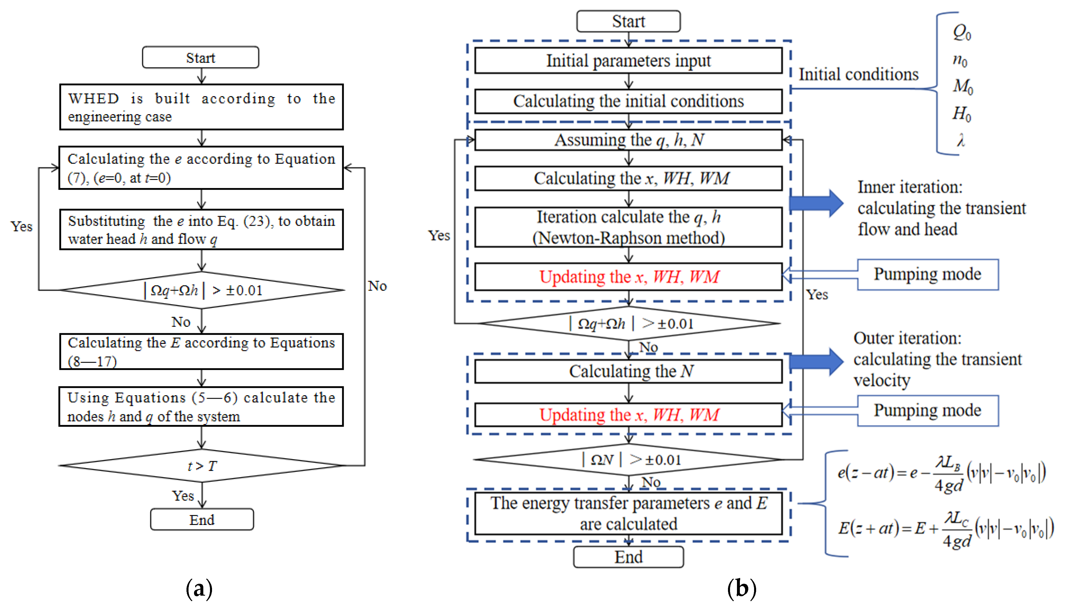
2. Method of Water Hammer Energy Difference (WHED)

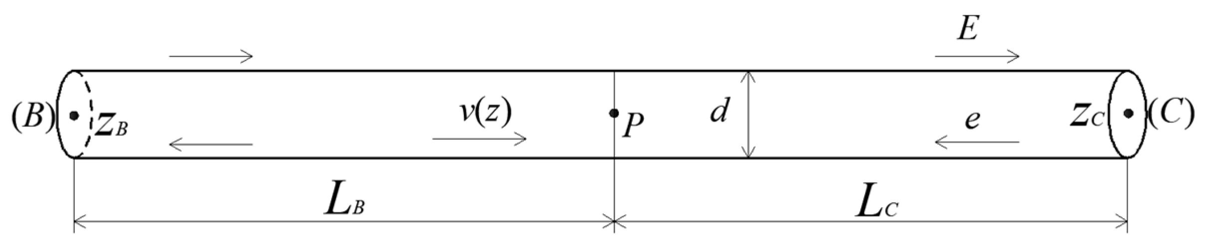
2.1. Fundamental Theory of WHED

The WHED simulates the generation, propagation, transmission, reflection, and attenuation of water hammer in a closed pipeline, based on the energy and continuity equations for unsteady flow. Transient parameters are calculated by analyzing the energy of the water hammer at each time step. Assuming that the pipe wall is an incompressible rigid body and the water inside the closed pipe is an ideal fluid, the fluid satisfies the equations of motion and continuity. Water hammer in pipes is essentially the transmission of pressure waves [37]. The fluid particle at any moment can be described by Equation (1). The energy of transient fluid at a certain moment consists of potential energy ${\displaystyle \frac{dH}{2}}$, kinetic energy ${\displaystyle \frac{adv}{2g}}$, and loss term ${\displaystyle \frac{\lambda dl}{2d}}{\displaystyle \frac{v\left|v\right|}{2g}}$.

$$dH\pm {\displaystyle \frac{a}{g}}dv+{\displaystyle \frac{\lambda v\left|v\right|}{2gd}}dl=0$$

(1)

The initial water head and flow velocity at the center of the pipe are defined as H₀ and v₀. H₀ and v₀ are substituted into Equation (1), making a difference with the current moment (H and v) results in Equation (2), which represents the energy change of a fluid particle in the pipeline. Equation (2) is the basic expression of WHED.

$${\displaystyle \frac{d}{dl}}\left({\displaystyle \frac{H-H_0}{2}}\pm {\displaystyle \frac{a}{2g}}\left(v-v_0\right)\right)=-{\displaystyle \frac{\lambda }{4gd}}\left(v\left|v\right|-v_0\left|v_0\right|\right)$$

(2)

Figure 2 shows a random fluid particle P in the pipeline, flanked by points B (L_B = z − z_B) and C (L_C = z_C − z), where the water flows from B to C. Integrating the length l in Equation (2) along the pipe yields Equations (3) and (4). Assuming the valve at B is closed, a positive wave in the same direction as the incoming flow appears to the right of B and propagates towards C. When this positive wave arrives at C, a negative wave is produced due to reflection, which propagates towards B in the opposite direction of the main flow. Thus, in the later analysis, a positive wave is directly caused by the movement of components like valves, whereas a negative wave is directly generated by the positive wave arriving at the next node. Defining $E={\displaystyle \frac{H-H_0}{2}}-{\displaystyle \frac{a}{2g}}\left(v-v_0\right)$ and $e={\displaystyle \frac{H-H_0}{2}}+{\displaystyle \frac{a}{2g}}\left(v-v_0\right)$ as transfer parameters of positive and negative energy, summing and differing E and e give Equations (5) and (6), respectively.

$${\displaystyle \frac{H-H_0}{2}}+{\displaystyle \frac{a}{2g}}\left(v-v_0\right)={\left[{\displaystyle \frac{H-H_0}{2}}+{\displaystyle \frac{a}{2g}}\left(v-v_0\right)\right]}_B-{\displaystyle \frac{\lambda L_C}{4gd}}\left(v\left|v\right|-v_0\left|v_0\right|\right)$$

(3)

$${\displaystyle \frac{H-H_0}{2}}-{\displaystyle \frac{a}{2g}}\left(v-v_0\right)={\left[{\displaystyle \frac{H-H_0}{2}}-{\displaystyle \frac{a}{2g}}\left(v-v_0\right)\right]}_C-{\displaystyle \frac{\lambda L_B}{4gd}}\left(v\left|v\right|-v_0\left|v_0\right|\right)$$

(4)

$$H-H_0=E+e$$

(5)

$$Q-Q_0=\pm {\displaystyle \frac{g}{aA}}\left(e-E\right)$$

(6)

In Equation (6), “−” is used when the pressure wave propagation direction is the same as the mainstream and “+” otherwise. Knowing the head, flow velocity, and wave velocity at the initial moment, the flow information at any moment can be solved by Equations (5) and (6). Substituting E and e into Equations (3) and (4) yields Equations (7) and (8), which describe the relationship among energy transfer parameters.

$$e\left(z-at\right)=e_B-{\displaystyle \frac{\lambda L_B}{4gd}}\left(v\left|v\right|-v_0\left|v_0\right|\right)$$

(7)

$$E\left(z+at\right)=E_C+{\displaystyle \frac{\lambda L_C}{4gd}}\left(v\left|v\right|-v_0\left|v_0\right|\right)$$

(8)

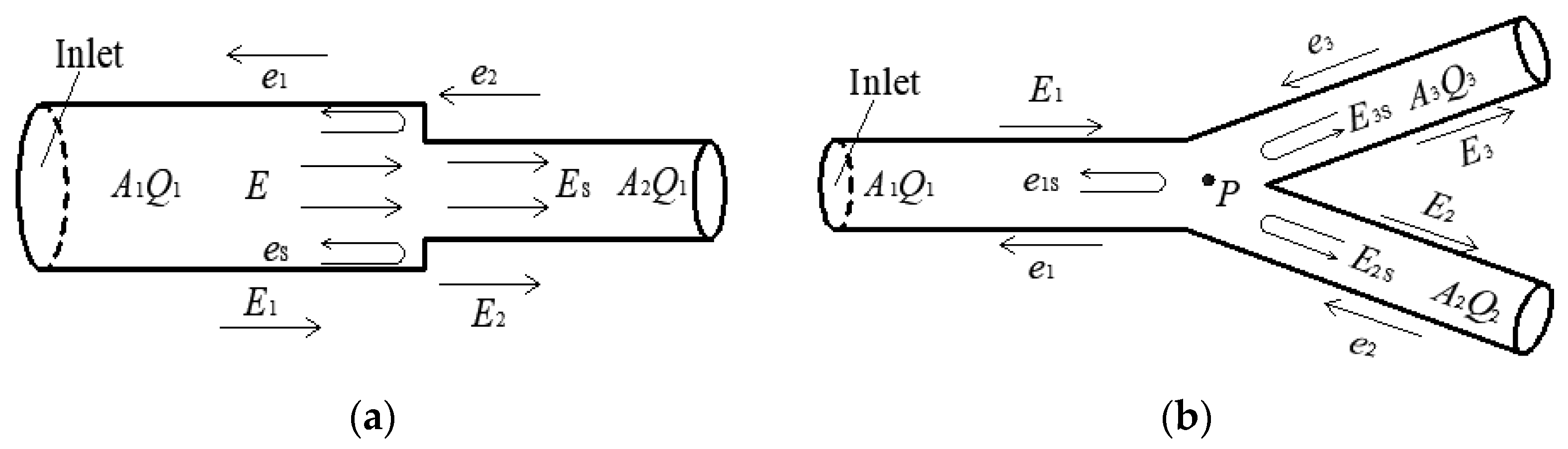
2.2. Pipeline with Varying Diameter and Bifurcated Conduit

Figure 3a shows a pipe with different diameters, where the flow direction is from A₁Q₁ to A₂Q₂. Part of wave energy E_S keeps propagation towards A₂Q₂, while the other part e_S travels in the opposite direction. Consequently, energy transfer parameters at the change in pipe diameter can be written as Equations (9)–(12).

$$E_1={\displaystyle \frac{H-H_0}{2}}-{\displaystyle \frac{a}{2g}}\left(v_1-v_{1,0}\right)$$

(9)

$$E_2={\displaystyle \frac{H-H_0}{2}}-{\displaystyle \frac{a}{2g}}\left(v_2-v_{2,0}\right)$$

(10)

$$e_1={\displaystyle \frac{H-H_0}{2}}+{\displaystyle \frac{a}{2g}}\left(v_1-v_{1,0}\right)$$

(11)

$$e_2={\displaystyle \frac{H-H_0}{2}}+{\displaystyle \frac{a}{2g}}\left(v_2-v_{2,0}\right)$$

(12)

E₁ and e₂ come from the previous node and can be solved directly using Equations (7) and (8). However, e₁ and E₂ are caused by the reflected waves. Solving these four equations jointly (Equations (9)–(12)) results in Equations (13) and (14).

$$e_1={\displaystyle \frac{A_1-A_2}{A_1+A_2}}{E}_1+{\displaystyle \frac{2A_2}{A_1+A_2}}{e}_2$$

(13)

$$E_2={\displaystyle \frac{2A_1}{A_1+A_2}}{E}_1+{\displaystyle \frac{A_2-A_1}{A_1+A_2}}{e}_2$$

(14)

Figure 3b displays a bifurcated conduit, where the flow direction is from A₂Q₂ to A₁Q₁ and A₃Q₃. Forward waves E₁, E₂, and E₃ move in the same direction as the mainstream, while the reflected waves e₁, e₂, and e₃ move in the opposite direction. e_1S, E_2S, and E_3S are parts of the reflected waves caused by E₁, e₂ and e₃, respectively, when E₁, e₂, and e₃ pass through point P. E₁, e₂, and e₃ come from the previous node, so they can be solved using Equations (7) and (8). e₁ is a confluence of e₂ and e₃, while E₁ is dispersed into E₂ and E₃. Thus, e₁, E₂, and E₃ can be solved using Equations (15)–(17), which are derived from Equations (9)–(12).

$$e_1={\displaystyle \frac{A_1-A_2-A_3}{A_1+A_2+A_3}}{E}_1+{\displaystyle \frac{2A_2}{A_1+A_2+A_3}}{e}_2+{\displaystyle \frac{2A_3}{A_1+A_2+A_3}}{e}_3$$

(15)

$$E_2={\displaystyle \frac{2A_1}{A_1+A_2+A_3}}{E}_1+{\displaystyle \frac{A_2-A_1-A_3}{A_1+A_2+A_3}}{e}_2+{\displaystyle \frac{2A_3}{A_1+A_2+A_3}}{e}_3$$

(16)

$$E_3={\displaystyle \frac{2A_1}{A_1+A_2+A_3}}{E}_1+{\displaystyle \frac{2A_2}{A_1+A_2+A_3}}{e}_2+{\displaystyle \frac{A_3-A_1-A_2}{A_1+A_2+A_3}}{e}_3$$

(17)

2.3. Boundary Conditions of Pump Turbine

The pump turbine is the core of a PSP, and the complete characteristic curves of the unit should be considered when determining boundary conditions. It is worth mentioning that this work also considered the energy transfer parameters from the upstream and downstream. The following Equations (18)–(20) belong to the improved Suter transfer method, used to quantitatively characterize the curves of a unit [38].

$$WH(x,y)={\displaystyle \frac{y^2}{{\left(n_{11}/n_{11r}\right)}^2+{\left(Q_{11}/Q_{11r}\right)}^2}}={\displaystyle \frac{h}{N^2+q^2}}{y}^2$$

(18)

$$WM(x,y)={\displaystyle \frac{M_{11}+k_1}{M_{11r}}}y=\left({\displaystyle \frac{m}{h}}+{\displaystyle \frac{k_1}{M_{11r}}}\right)y$$

(19)

$$x=\left\{\begin{array}{c}\hfill \arctan \left({\displaystyle \frac{Q_{11}/Q_{11r}+k_2}{n_{11}/n_{11r}}}\right)=\arctan \left({\displaystyle \frac{q+k_2\sqrt{h}}{N}}\right), N\ge 0\hfill \\ \hfill \pi +\arctan \left({\displaystyle \frac{Q_{11}/Q_{11r}+k_2}{n_{11}/n_{11r}}}\right)=\pi +\arctan \left({\displaystyle \frac{q+k_2\sqrt{h}}{N}}\right), N<0\hfill \end{array}\right.$$

(20)

The positive wave near the upstream side of the pump turbine does not reach the next node at the initial time, so it has no reflected waves, meaning e₁ = 0. Similarly, the pump turbine near the downstream has e₂ = 0. Combining e₁ = 0 and e₂ = 0 with Equations (5) and (6) yields Equations (21) and (22). Ignoring the main losses of the pump turbine, such as hydraulic, volume, and mechanical losses, $H_t=H_1-H_2$. Substituting Equations (21) and (22) into $H_t=H_1-H_2$ results in Equation (23), which is the expression of the pump turbine boundary.

$$H_1-H_{1,0}=2e_1-{\displaystyle \frac{a\left(Q_1-Q_{1,0}\right)}{A_{1}g}}$$

(21)

$$H_2-H_{2,0}=2e_2+{\displaystyle \frac{a\left(Q_2-Q_{2,0}\right)}{A_{2}g}}$$

(22)

$$h{H}_r=2\left(e_1-e_2\right)-{\displaystyle \frac{a_1}{A_{1}g}}\left(q{Q}_r-Q_{t0}\right)+{\displaystyle \frac{a_2}{A_{2}g}}\left(q{Q}_r-Q_{t0}\right)+H_{1,0}-H_{2,0}$$

(23)

Equation (23) uses subscripts 1 and 2 to distinguish the parameters near the upstream side and downstream side, while the subscript 0 represents the initial time.

3. Validation of WHED in an HP

The WDS of one HP is built in the lab, as shown in Figure 4a. The arrangement consists of one pipe and three machines, and the schematic is shown in Figure 5 and the pipeline parameters are shown in

Table 1. Pipeline parameters of the WDS.

Number	Length (m)	Pipe Diameter (m)	Area (m2)	Wave Velocity (m/s)	Roughness
1	493.42	11	94.99	1319	0.015
2	7.8	11	94.99	1319	0.015
3	19.3	6.35	31.65	1157.66	0.012
4	65.55	6.35	31.65	1157.66	0.012
5	53.20	6.35	31.65	1157.66	0.012
6	19.3	6.35	31.65	1157.66	0.012
7	65.55	6.35	31.65	1157.66	0.012
8	53.20	6.35	31.65	1157.66	0.012
9	19.3	6.35	31.65	1157.66	0.012
10	65.55	6.35	31.65	1157.66	0.012
11	53.20	6.35	31.65	1157.66	0.012

. The placement of the pressure sensors is described in a previous study [31], and three valves are used to control the flow. To accurately capture the dynamic variation of water hammer pressure in the pressure pipeline, the physical model utilizes both pressure sensors and a high-speed camera to collect pressure and surge water level data in the surge tank. More than 40 pressure sensors are installed in the test rig. This study primarily focuses on the validation of calculations using the pressure sensors H₁, H₂, and H₃, located at the downstream end of pressure pipelines No. 1 to No. 3, as shown in Figure 4a, along with the pressure sensor H_B at the bottom of the surge tank. Additionally, the surge water level H_W recorded by the high-speed camera is also validated. The following four points are included in this experiment:

(1)

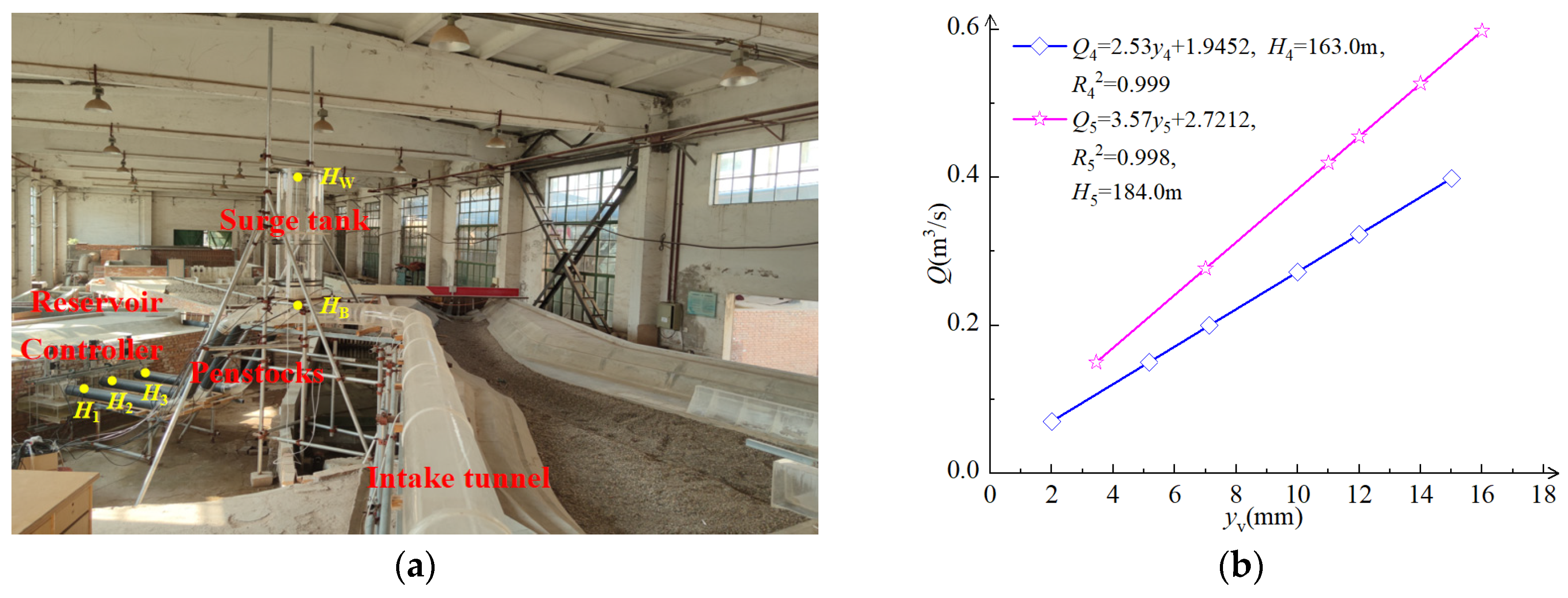
The overflow weir regulates the water level in the upper reservoir, and the flow rate is determined by the gauging weir in conjunction with the regulating valve.

(2)

A high-speed camera records the changes in waves within the surge tank.

(3)

The signal acquisition system monitors from 0 to 350 s.

(4)

The wave velocity a is measured by quickly cutting off the water flow using a gate to produce water hammer waves. The pressure sensors at both ends of the pipe record the first wave time t₁, which is used to calculate the water hammer wave velocity (a = l/t₁).

In order to ensure that the model experiment can accurately reflect the operation of the actual project, the model test is designed with the Froude criterion. The relationship of the water hammer wave velocity scale (${\delta }_c$) and the geometric scale (${\delta }_l$) is ${\delta }_c={\delta }_l^{0.5}$. The water hammer wave velocity of the pressure pipe is 1157.66 m/s, which is obtained by considering the hydropower station (1100 m/s). The difference is caused by pipe materials, which is polyvinyl chloride (PVC).

To capture the transient characteristics in the WDS, pressure sensors with a range of 0–100 kPa are arranged at different locations in the pipelines and the surge well, and a video camera is used to record the changing water level in the surge [31]. Pressure signals are collected by a directly attached storage system, and sampling frequency of all sensors is 1000 Hz. The geometric scale of the test model is 42.87.

This paper analyzes the transient characteristics at five special positions, as shown in Figure 4a: H₁, H₂, and H₃ are located at the end of the WDS; H_B is at the bottom of the surge tank; and H_W represents the wave in the surge tank. Detailed information on the four transitions is shown in

Table 2. Four transient conditions of HP.

Conditions	Description
ET1	Upstream reservoir—184 m, three units rejecting loads at the same time
ET2	Upstream reservoir—163 m, three units rejecting loads at the same time
ET3	Upstream reservoir—184 m, two units operating at full load, one unit increasing to full load, and then three units rejecting loads at the same time
ET4	Upstream reservoir—163 m, two units operating at full load, one unit increasing to full load, and then three units rejecting loads at the same time

, where 163 m and 184 m are the minimum and normal storage levels of the upper reservoir in the HP, respectively.

Figure 4b shows the flow control laws under different conditions. The trend of the test results is linear. In Equation (24), R² is the linear correlation coefficient, sum of squares of residuals (SSR) and total sum of squares (TSS) are the regression and total sum of squares, respectively. Both SSR and TSS are greater than 0.99, indicating that the accuracy of the test bench control module is high.

$$R^2=1-{\displaystyle \frac{SSR}{TSS}}$$

(24)

The application steps of WHED in HP are shown in Figure 6a, where Ωq, Ωh, and ΩN represent the differences between the predicted and calculated values. Figure 6b illustrates the calculation procedure of the transient conditions detailed in this paper. It should be noted that the red steps in Figure 6b are not included in the research in generating mode (conditions of the turbine model are in the first quadrant).

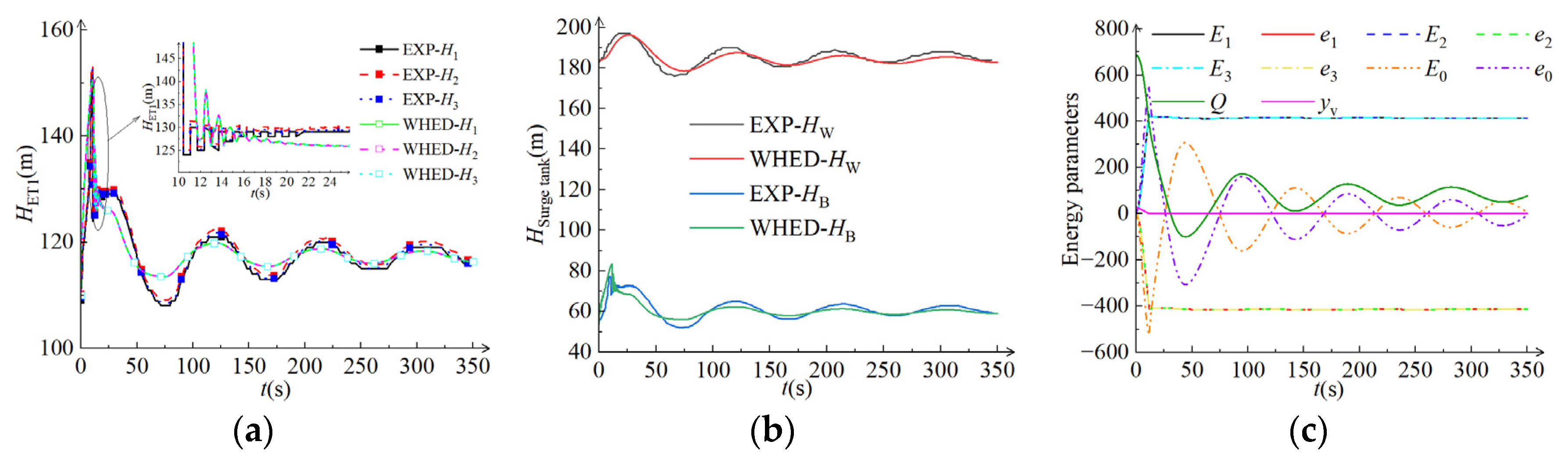
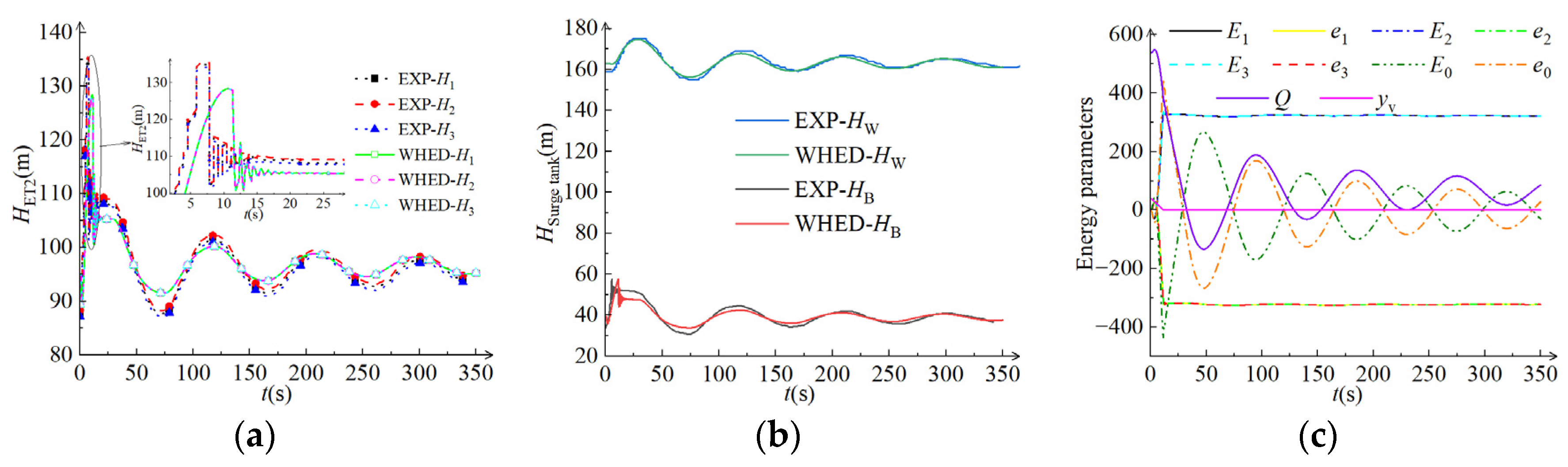
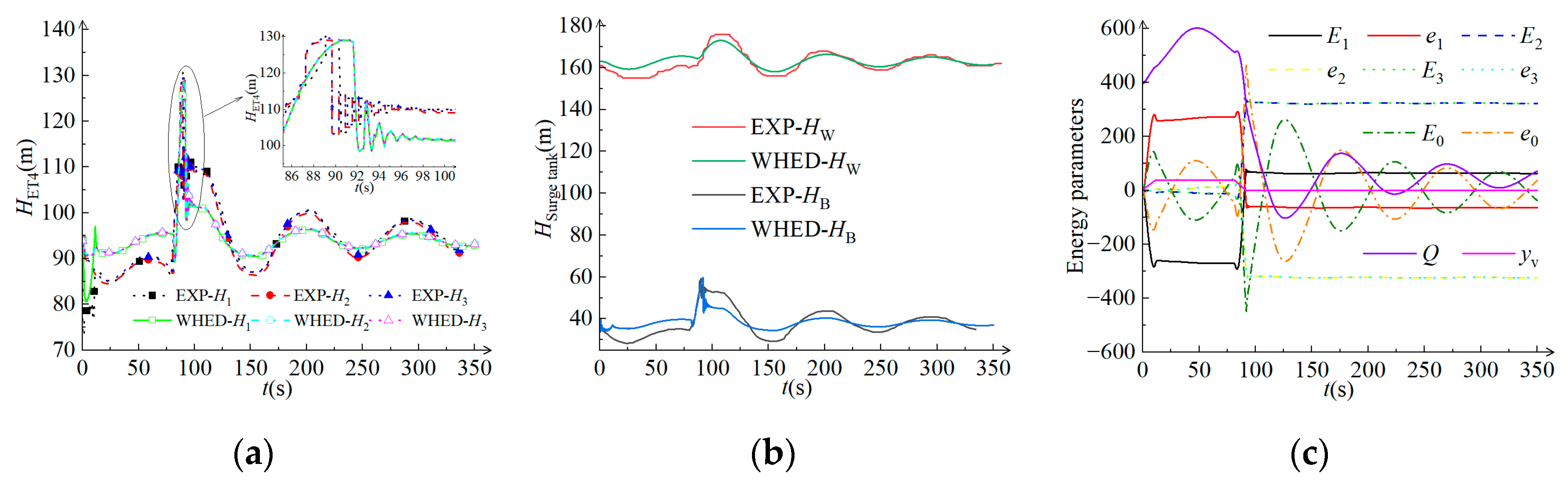
3.1. Comparative Analysis of Numerical and Experimental Results

The calculating data of WHED are consistent with the experiment results. Defining ${\Delta }_1={\displaystyle \frac{\left|WHED-Experiment\right|}{Experiment}}\times 100\%$ to measure the difference between the experiment and WHED, Δ_1max of H is only 4.8%. The model pipe in the laboratory is made of PVC for measuring wave velocity, while the hydropower plant uses steel for the WDS. Due to the different elastic moduli of the two materials, their wave velocities differ. In this work, the wave velocity of the steel pipe used in the plant is adopted, which results in the calculated values slightly lagging behind the experimental data. Validation of numerical simulations has been completed in the previous stage [31].

Pressure changes at the end of the WDS and the water level in the surge tank of ET1 are shown in Figure 7a,b. Valve closure causes a rapid rise in pressure at the end of the WDS (H_max = 153 m). Part of the water flows into the surge tank, causing H_W to start increasing while H₁, H₂, and H₃ gradually decrease. After four waves, H_B and H_W reach stable values (H_wmax = 198 m), with Δ_1max of H_w being only 1.1%.

The changes in valve opening (y_v), flow rate (Q), and energy transfer parameters (E and e) are shown in Figure 7c. The subscripts 1, 2, and 3 indicate the energy transfer parameters at the end of three pipelines of the WDS, while the subscript 0 represents the surge tank. e increases in the negative direction when E reaches the reservoir end. The reflection flow (e) arrives at the end of pipes at t = 1.1, then a positive direct water hammer appears in the pipeline because the valves have not been fully closed, accompanied by a rapid rise in pressure at the ends of pipes. E₀ and e₀ at the surge tank increase in the negative and positive directions, respectively, exhibiting opposite trends compared with E and e at pipe ends, which is consistent with the regulating function of the surge tank. The shrinking fluctuations of E₀ and e₀ after their maximum values are caused by oscillatory changes in flow.

Figure 8 shows that ET2 has a similar situation to ET1, but the maximum H at the end of WDS and H_w are 18 m and 20 m smaller than those in ET1, primarily due to different reservoir levels (H_R). The pressure at each position experiences four waves before stabilization, with Δ_1max of H at the end of the WDS being about 4.9% and Δ_1max of H_w around 1.8%. The trends of the energy transfer parameters for ET1 and ET2 illustrate the key role played by the surge tank for pressure stabilization within the system.

Valve closure at the pipe ends brings the flow to 0, causing E₁, E₂, and E₃ to first increase and then stabilize. However, the surge fluctuation in the regulating well leads to pulsations in E₀ and e₀, with their pulsation amplitudes gradually shrinking and stabilizing, as shown in Figure 8c. These reasons also apply to the changes in energy parameters in the later figures of this case.

H at the end of the WDS and H_W and H_B exhibit different change trends in Figure 9. Firstly, the pressure of H₁ decreases due to the larger valve opening from t = 0 to 75 s (H_1min = 105 m), accompanied by smaller H_W and H_B. The pressure at H₂ and H₃ experiences small fluctuations from t = 0 to 75 s (H_min = 113 m), influenced by the surge tank. e₀ decreases and then increases at the startup of one unit, reflecting the change in water flow in the surge tank from outflow to inflow.

At t = 75 s, three units start to reject the full load, causing a rapid pressure rise (H_max = 146 m) similar to ET1. However, the maximum H is smaller in ET3 than in the simple load rejection condition, as pressure fluctuations at the end of the load increase offset some of the fluctuations at the beginning of load rejection. After t = 75 s, e₀ rises and then falls, with its subsequent three waveforms gradually decaying. The changing trends of WHED and experimental results are essentially the same, with Δ_1max of H₁, H₂ (H₃), and H_w being 6.9%, 6.8%, and 3.3%, respectively.

As Figure 10 shows, the changing characteristics of ET4 under both WHED and experimental conditions are similar to ET3. The maximum pressure at the end of the WDS of ET4 is 15 m smaller than in ET3, for the same reason as the difference between ET1 and ET2, caused by lower H_R. Δ_1max of H₁, H₂, and H₃ are approximately 4.6%, while Δ_1max of H_w is 3.8%. H_w of the surge tank first drops and then rises, with a total of four waveforms appearing in the two stages. Compared with ET3, H_wmax is reduced by 19 m.

WHED is utilized in four transient conditions of HP. Compared to the experimental results, the maximum error Δ_1max of each parameter is smaller than 7%, demonstrating the good reliability of WHED. The reservoir level significantly affects the pressure fluctuation amplitude (lower H_R corresponds to smaller maximum values), but it has no effect on the pressure development trends.

3.2. Stability Analysis of Pressure Parameters in WDS of HP

Multidimensional scaling (MDS) is employed to quantitatively analyze the parameters from the transient conditions listed in Table 2, defining u in Equation (25) as a measure of safety, where u₁ is the fluctuating amplitude of parameters as shown in Equation (26), and u₂ denotes the change rate of parameters as expressed in Equation (27).

u = c₁u₁ + c₂u₂

(25)

$$u_1={\displaystyle \frac{\left|c_{\max }\right|-c_r+\left|c_{\min }\right|-c_r}{2}}$$

(26)

$$u_2={\displaystyle \frac{c_{\max }-c_0}{t}}$$

(27)

In the above two expressions, c_max, c_min, and c_r are the maximum, minimum, and rated values of H₁, H₂ (H₃), and H_w, respectively. $c_1={\displaystyle \frac{{\overline{u}}_1}{{\overline{u}}_1+{\overline{u}}_2}}$, $c_2={\displaystyle \frac{{\overline{u}}_2}{{\overline{u}}_1+{\overline{u}}_2}}$, ${\overline{u}}_1$ and ${\overline{u}}_2$ are the average values of u₁ and u₂. A larger u₁ indicates a greater change in parameters, while a bigger u₂ signifies a faster change in parameters.

Table 3. u₁, u₂, and u of four transitions in Table 2.

Conditions	H1			H2 (H3)			Hw
	u1	u2	u	u1	u2	u	u1	u2	u
ET1	19.51	3.71	17.14	19.61	3.71	16.91	8.82	0.49	8.49
ET2	19.65	3.56	17.24	19.05	3.56	16.42	9.09	0.42	8.74
ET3	19.92	3.88	17.51	15.84	3.83	13.79	7.17	0.12	6.89
ET4	22.06	3.65	19.29	18.92	3.72	16.34	6.84	0.17	6.57

lists the calculated results of u₁, u₂, and u for the transitions in Table 2.

The u₁ of H₁ follows the order ET4 > ET3 > ET2 > ET1, demonstrating that the load regulation mode significantly influences the flow regime. During ET3 and ET4, where one unit increases to full load and then rejects the full load, the u₁ of wave superposition pulsation in these two phases is larger compared to ET1 and ET2. The magnitude pattern of u₂ for H₁, H₂, and H₃ is consistent with u₁. Notably, u₁ and u₂ of H₁ at lower reservoir levels (ET2 and ET4) are higher, while u₁ and u₂ of H₂ and H₃ show the opposite trend. The u values of H₁ are consistently higher than the u values of H₂ and H₃, which indicates that H₁ has stronger fluctuations than H₂ and H₃. The difference in u from H₁, H₂, and H₃ in ET1 and ET2 conditions is less than 1, while the difference in u from H₁, H₂, and H₃ in ET3 and ET4 conditions is about 3, which illustrates that the combined condition (first increasing and then decreasing the load) has a larger pressure fluctuation compared with a single process with load decrement. This further highlights the important impact of load regulation patterns on system safety.

A comprehensive parameter $\overline{u}$ is defined as the weighted average values of q, h, and N in Equation (28). Here, ${\overline{u}}_{H_1}$, ${\overline{u}}_{H_2(H_3)}$, and ${\overline{u}}_{H_w}$ are the average values of u from H₁, H₂ (H₃), and H_w. $c={\overline{u}}_{H_1}+{\overline{u}}_{H_2(H_3)}+{\overline{u}}_{H_w}$, and the calculating results of these quantities are presented in

Table 4. The weighted values of H₁, H₂ (H₃), and H_w.

Conditions	${\overline{\mathit{u}}}_{{\mathit{H}}_1}/\mathit{c}$	${\overline{\mathit{u}}}_{{\mathit{H}}_2({\mathit{H}}_3)}/\mathit{c}$	${\overline{\mathit{u}}}_{\mathit{H}\mathit{w}}/\mathit{c}$	$\overline{\mathit{u}}$
ET1	7.34	6.60	1.53	15.47
ET2	7.13	6.40	1.52	15.05
ET3	7.46	5.38	1.26	14.10
ET4	8.22	6.37	1.18	15.77

. From a comprehensive perspective, the safety order of the conditions in Table 1 is ET3 > ET2 > ET1 > ET4. ET3 exhibits the best performance, while ET4 represents the worst case, with the latter value of $\overline{u}$ being reduced by 1.67 compared to the former condition.

$$\overline{u}={\displaystyle \frac{{\overline{u}}_{H_1}}{c}}+{\displaystyle \frac{{\overline{u}}_{H_2(H_3)}}{c}}+{\displaystyle \frac{{\overline{u}}_{H_{\mathrm{w}}}}{c}}$$

(28)

3.3. Coupled Computation of 1D WHED with 3D Numerical Simulation

The one-dimensional water hammer energy difference calculation method is coupled with the three-dimensional numerical simulation method to calculate the time-dependent variations of flow parameters in the diversion system of a hydropower station. The flow rate at the inlet of the diversion pipe and the pressure at the end of the pressure pipeline are calculated using the one-dimensional energy difference method, which then serves as the boundary conditions for the 3D numerical simulation. A 3D model of the diversion system is established, and meshing is performed. As shown in Figure 11a, five grid configurations (2.6 million, 4.15 million, 5.78 million, 6.0 million, 6.3 million) were tested for grid-independence validation, using the ratio of H/HEXP as the evaluation criterion (where H and HEXP represent the numerical and experimental heads, respectively). When the grid count reached 5.78 million, the H/HEXP ratio stabilized.

A steady state was achieved by filling the diversion system with water, a task completed in previous work [30]. Based on this, the coupled calculation was performed by transferring data from the 1D water hammer energy difference method to the 3D numerical simulation in a one-way manner, while monitoring the surge level in the regulating well during the 1D–3D coupled calculation. Figure 11b presents the comparison between the one-dimensional and three-dimensional coupled results and the model test results for four experimental conditions. The water level trends in the regulating well are largely consistent. The maximum computational deviation for the four experimental conditions is approximately 1.9%, indicating good coupling performance.

The turbulence kinetic energy (TKE) in the diversion system for each experimental condition is shown in Figure 12a–d, with each image depicting the moment when the water level in the regulating well reaches its maximum value. Conditions ET1 and ET2 represent load shedding scenarios, with the turbulence intensity in ET2 being more severe than in ET1. Conditions ET3 and ET4 involve first increasing load and then shedding load, where the turbulence intensity in ET4 is more pronounced than in ET3. This indicates that turbulence in the regulating well is more intense under low water level transition conditions. High-TKE regions are concentrated around the impedance holes, where the turbulence intensity is most severe. In all four conditions, irregular flow extends from the impedance hole into the regulating well, with turbulence intensity gradually decreasing as it is influenced by the water pressure in the regulating well. The maximum turbulent kinetic energy in the low-water conditions, ET2 and ET4, is higher than that in the high-water conditions, ET1 and ET3, with the maximum TKE value being approximately twice that of ET1 and ET3.

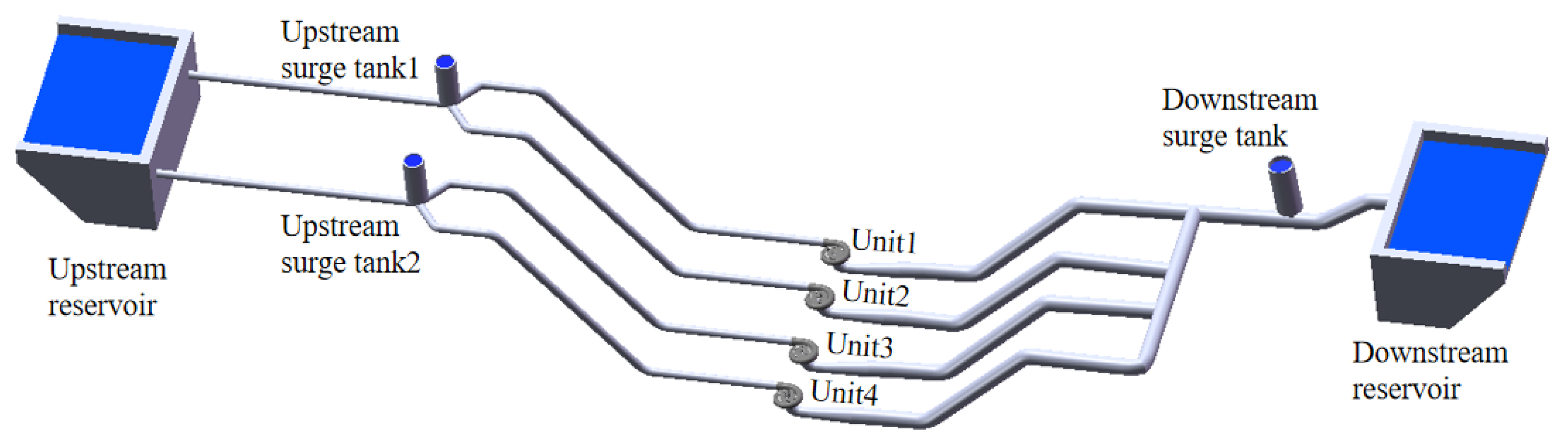
4. Validation and Application of WHED in a Pumped Storage Plant

An operating PSP in China is depicted in Figure 13. Since its commissioning and operation until the end of 2020, this PSP has consumed a total of 9.578 billion kW·h of clean energy and has generated a total of 7.833 billion kW·h of electricity. Eight frequently used transient conditions of the PSP case are investigated using WHED, as shown in

Table 5. Typical transitions.

Designation	Transitions	Description
TC0	Load rejection (Generation mode)	Upstream reservoir—normal water level Initial state—the rated condition Load rejection—guide vanes spend 15 s from 100% to 10% opening
TC1	Load increment (Generation mode)	Upstream reservoir—normal water level Initial state—generating mode with 30% load Load increment—guide vanes spend 20 s from 30% to 100% opening
TC2	Load reduction (Generation mode)	Upstream reservoir—normal water level Initial state—the rated condition Load reduction—guide vanes spend 15 s from 100% to 30% opening
TC3	Shutdown (Generation mode)	Upstream reservoir—normal water level Initial state—the rated condition Shutdown—guide vanes spend 15 s from 100% to 10% opening
TC4	Startup (Generation mode)	Upstream reservoir—normal water level Initial state—shutdown Shutdown—guide vanes spend 20 s from 10% to 100% opening
PC0	Power outage (Pumping mode)	Downstream reservoir—normal water level Initial state—the rated condition Shutdown—guide vanes spend 15 s from 50% to 10% opening
PC1	Shutdown (Pumping mode)	Downstream reservoir—normal water level Initial state—the rated condition Shutdown—guide vanes spend 40 s from 50% to 10% opening
PC2	Startup (Pumping mode)	Downstream reservoir—normal water level Initial state—shutdown Shutdown—guide vanes spend 12 s from 10% to 50% opening

. The validation cases include critical working conditions such as load rejection under generating mode (TC0) and accidental power outage under pumping mode (PC0). This Chinese PSP includes upper and lower reservoirs, two water diversion systems with two upstream surge tanks, four units, and one downstream surge tank on the pipeline between the unit and lower reservoir. Both MOC and WHED are employed to calculate the parameter changes under transient conditions. The computational programs for MOC and WHED were completed in a previous study by the authors [39]. The operation process of WHED and the calculation procedure of transitions are shown in Figure 6.

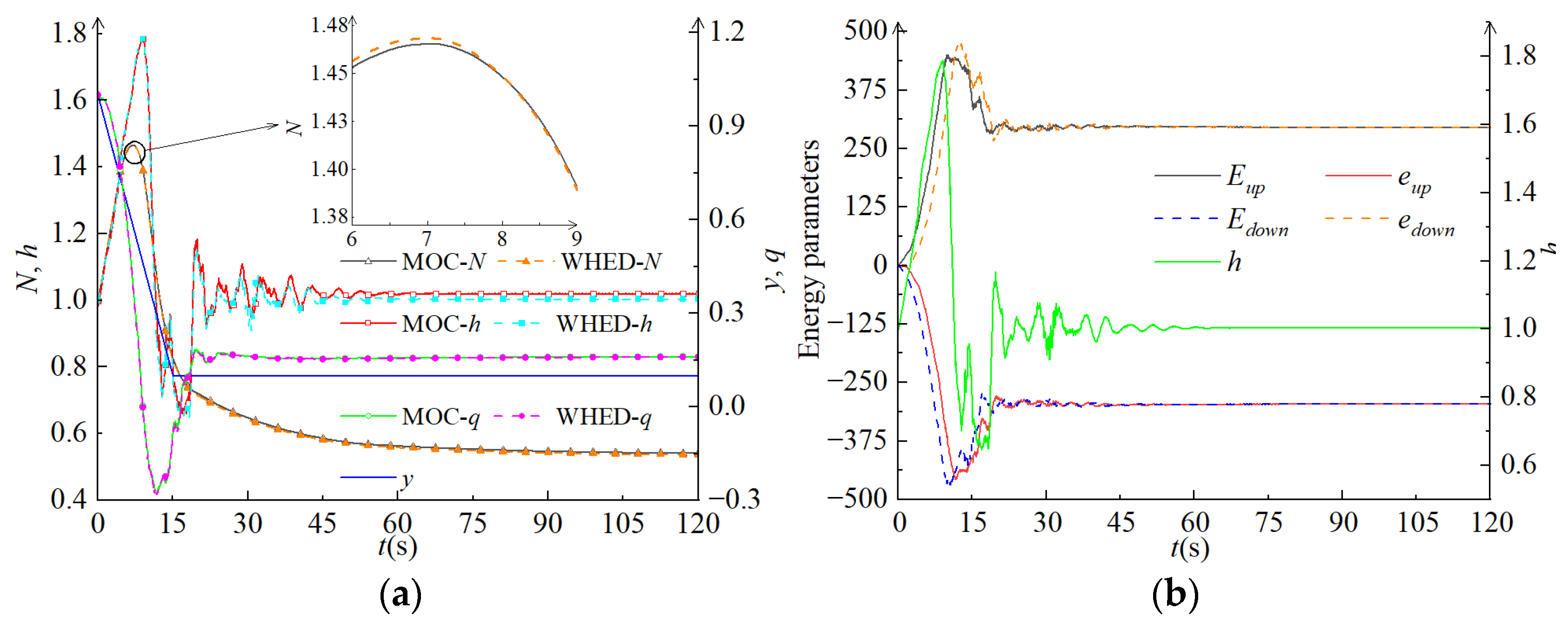
4.1. Validation of Dangerous Working Conditions

Figure 14a,c present the complete characteristic curves of the pump turbine belonging to the PSP shown in Figure 13, while Figure 14b,d display the modified forms using the Suter method, which will be used in subsequent calculations. S₁ in Figure 14a represents the initial point of TC0, corresponding to the normal water level in the upper reservoir and the rated condition of the turbine. During TC0, guide vanes take 15 s to move from y₀ to 10% y₀, following the guide vane closure law y = 1 − 0.06t. S₂ in Figure 14a marks the initial state of PC0, where the lower reservoir is at the normal water level and the pump operates under rated conditions. In PC0, the guide vanes take 15 s to move from 50% y₀ to 10% y₀, with the guide vane closure law y = 0.5 − 0.0267t. For PC0, a braking mechanism can be used to stop the hydraulic machine quickly in emergency situations, although shutting down by guide vane closure is a comparatively longer process.

Figure 15a demonstrates the fluctuations in rotation speed, torque, and mass-flow during TC0. The flow continues to decrease until it reaches 0 at t = 8.9 s. Subsequently, a reflux appears in the system, reaching a maximum value of q_max = −0.285, and it takes 30 s to stabilize at q = 0.155. The rotation speed increases sharply and then decreases (N_max = 1.47 at t = 7 s) due to the unit experiencing runaway before braking during the load rejection period. The pressure initially rises and then falls (h_max = 1.79, h_min = 0.66). The first wave ends at t = 19 s, followed by small pressure fluctuations around h = 1. These fluctuations persist for about 45 s, as the unit’s operating point repeatedly passes through the braking zone and the reverse pump zone at the end of the load rejection process. In addition, the water level pulsation causes the pressure to converge more slowly compared to the flow and rotation speed.

The vector sum of positive and negative energy transfer parameters corresponds the pressure change between the initial moment and any given time (Equation (5)). Figure 15b illustrates that the forward and reflected waves in the pipelines exhibit similar change patterns, with initial upward trends followed by downward tendencies, ultimately leading to the stabilization of all variables. The differences in parameter values and propagation times are primarily attributed to variations in pipe lengths and the discrepancies in the energy carried by each pressure wave. For instance, as shown in Figure 15b, near the upstream region, E_up > 0, e_up < 0, and the vector sum of E_up and e_up > 0, indicating the occurrence of a positive water hammer. E_up reaches its maximum value at t = 10.1 s, coinciding with the first peak in pressure h. E_up decreases immediately after t = 10.1 s. The change in e_up is similar to E_up, but with an opposite value, causing their vector sum to gradually declines, indicating a pressure reduction. e_up reaches its maximum at t = 11.8 s, corresponding to the first trough in pressure h. After t = 12.4 s, minor fluctuations appear in the curves of E_up and e_up, which correspond to small fluctuations in h. The vector sum of E_up and e_up equals 0 at t = 60 s, demonstrating that the system has reached a new stable operating state. The water hammer phenomenon on the downstream side is completely opposite to that on the upstream side. On the upstream side, the initial water hammer pressure wave moves counter to the mainstream direction, whereas on the downstream side, it aligns with the mainstream direction.

Figure 16 illustrates the continuous decrease in rotation speed under the PC0 condition. After t = 43.3 s, the unit enters the reverse pump zone, where it begins rotating in the opposite direction, with its rotation speed increasing to around N = 0.557. The initial sharp drop in rotational speed is caused by the disconnection between the motor and the unit. Subsequently, the unit begins to rotate in the opposite direction, leading to increased reflux, which causes the unit to enter the turbine zone in reverse and accelerate toward a runaway condition. The flow declines from the beginning until t = 7.11 s, when backflow appears at the unit outlet. The main cause of this backflow at t = 7.11 s is the unit entering the braking zone, where the rotation speed reaches 0. The maximum backflow is q_max = 0.3 at t = 10.4 s and eventually stabilizes at approximately q = 0.16.

Figure 16b shows that E_up < 0 and e_up > 0, with the vector sum of E_up and e_up < 0, indicating the presence of a negative water hammer in the system. E_up decreases to a minimum at t = 9.93 s, while e_up initially increases, causing their sum to rise slowly and resulting in an upward trend in pressure. At t = 11.28 s, corresponding to the maximum value of e_up, the pressure h reaches its peak value. Small fluctuations in E_up and e_up are observed under both critical conditions (TC0: −294.4 to −327.4 and PC0: 294.5 to 328.2). Following the first waves of E_up and e_up, the pressure fluctuates within the range of 0.985 to 1.145 during this stage. The sum of E_up and e_up reaches 0 after 106.5 s under the PC0 condition, indicating that the system has reached a new stabilized state.

To measure the differences between MOC and WHED, the relative error ${\Delta }_2={\displaystyle \frac{\left|WHED-TLM\right|}{TLM}}\times 100\%$ is calculated as the absolute difference between MOC result and WHED result, divided by MOC. Two partial enlargements in Figure 15a and Figure 16a show N (Δ₂ = 0.2%) at TC0 and h (Δ₂ = 1.8%) at PC0 calculated by WHED and MOC, respectively.

Table 6. Comparison between WHED and MOC under TC0 and PC0.

		Nmax	Nmin	hmax	hmin	qmax	qmin
	WHED	1.469	0.541	1.796	0.673	1.010	−0.277
TC0	MOC	1.465	0.537	1.794	0.659	1.000	−0.285
	Δ2	0.2%	0.7%	0.1%	1.9%	1.0%	2.8%
	WHED	0.560	−0.957	1.305	0.543	0.301	−0.709
PC0	MOC	0.557	−0.956	1.297	0.533	0.298	−0.717
	Δ2	0.5%	0.1%	0.6%	1.8%	1.0%	1.1%

shows the other parameters’ Δ₂. The minor differences at TC0 are: Δ_2N = 0.7%, Δ_2h = 1.9%, and Δ_2q = 2.8%. The minor differences at PC0 are: Δ_2N = 0.5%, Δ_2h = 1.8%, and Δ_2q = 1.1%. Table 2 also elaborates that the Δ₂ values of N_min, h_min, and q_min are larger at TC0 than that at PC0, whereas the Δ₂ values of N_max, h_max, and q_max are vice versa. The Δ₂ is smaller than 3%, which interprets the credibility of WHED. Furthermore, WHED has several advantages over MOC:

(1)

WHED adopts energy transfer parameters from the initial and calculating time, using Equations (3)–(8) to derive boundary equations that solve the system. However, MOC uses two adjacent nodes at the previous moment to build the characteristic functions for the calculating moment. The functions constructed by each pair of nodes are generally different, making MOC more complicated than WHED.

(2)

WHED has better timeliness because it only needs to calculate the boundary conditions of the two endpoints of the target segment. By dynamically considering the wave propagation time, WHED allows for a larger time step, significantly improving computational efficiency. Conversely, MOC requires dividing the pipeline into multiple sections and constructing equations with adjacent nodes, requiring a smaller time step and the processing of a large amount of unnecessary nodes.

(3)

WHED provides a clear physical interpretation by analyzing changes in energy transfer parameters to explain pressure changes under transient conditions. However, MOC relies on characteristic equations based on the finite difference method, which do not directly characterize the causes of changes in the system’s flow regimes.

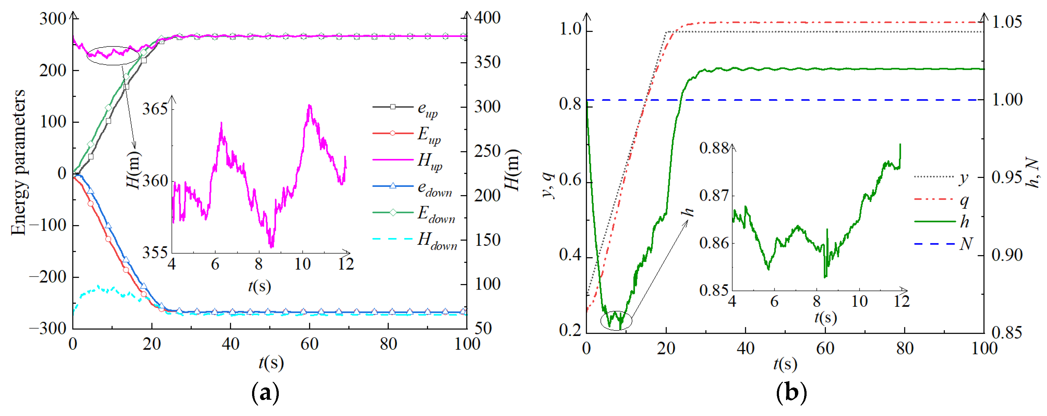
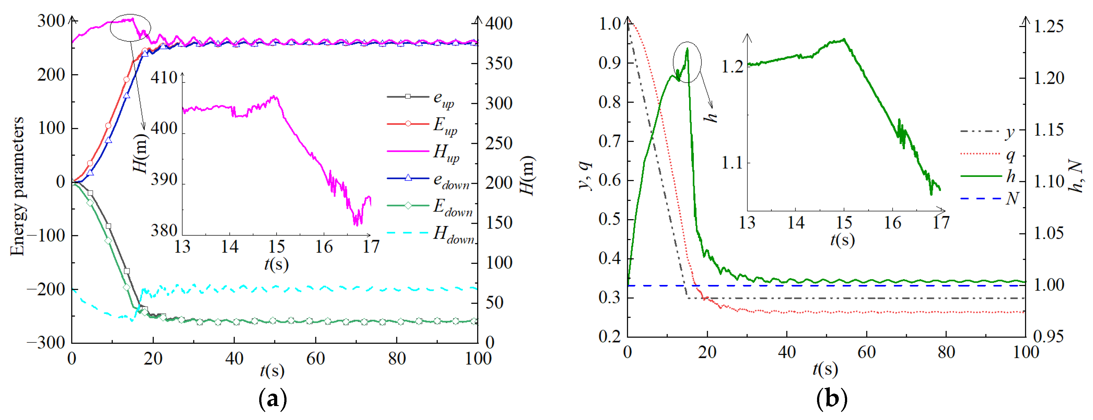
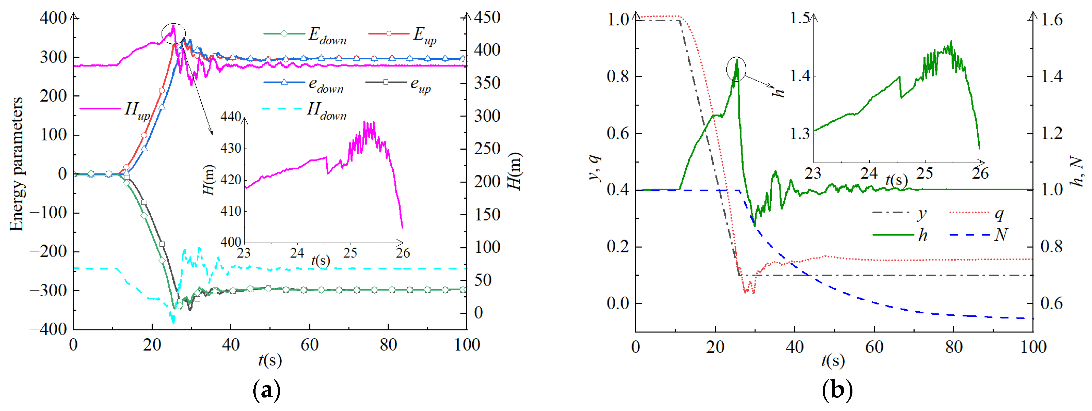
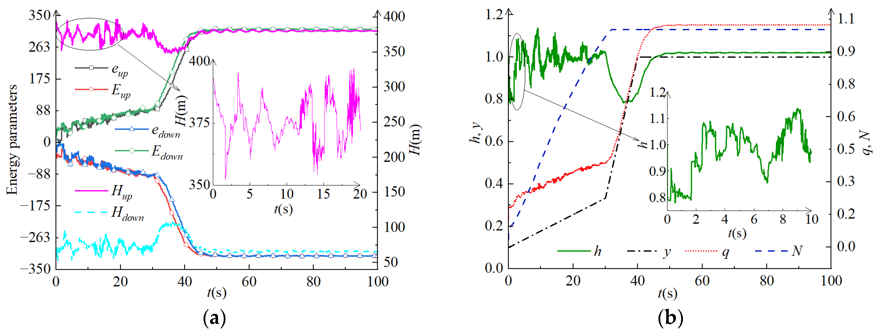
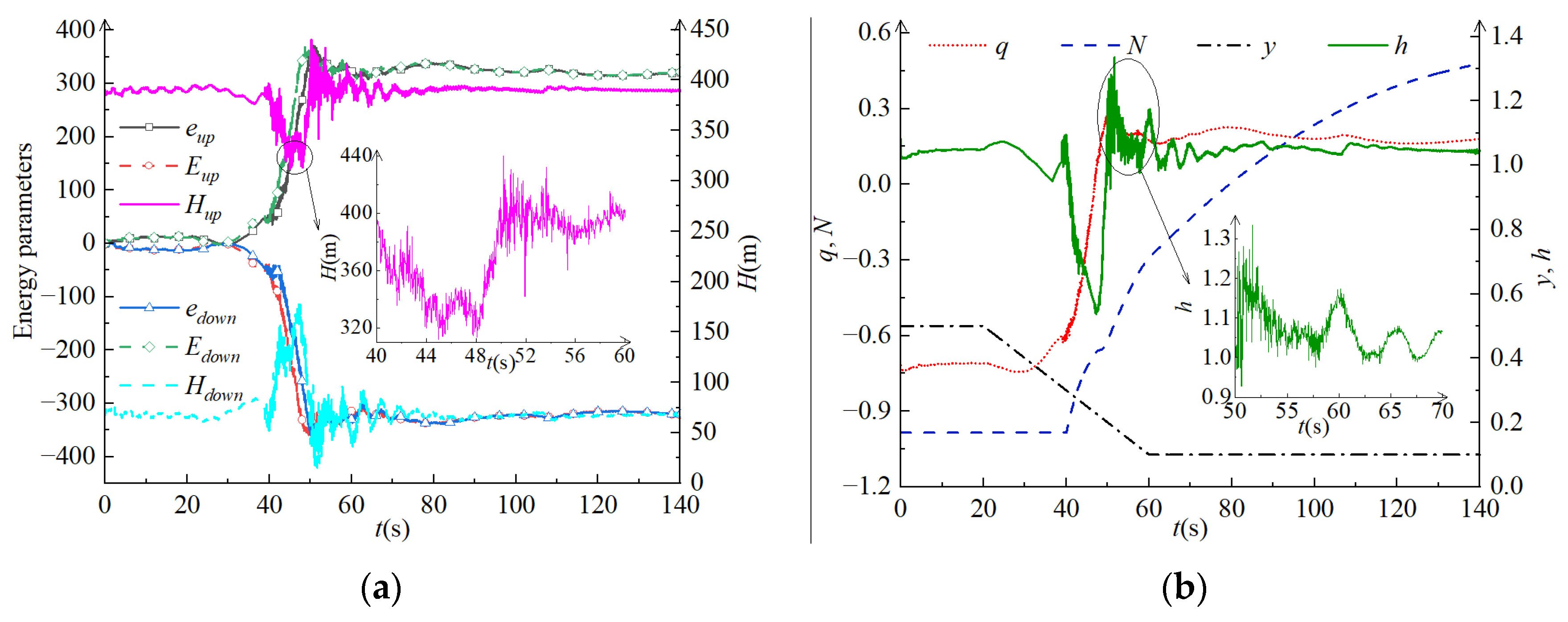
4.2. Calculation and Analysis of Generation Conditions

Figure 17a shows the continuous movement of the guide vane (y = 0.035t + 0.3) at TC1. Taking the upstream side as an example, the sum of E_up and e_up < 0 indicates the occurrence of a negative water hammer on the upstream side. E_up < 0 and the water hammer wave is a decompression wave, and the negative waves are reflected from positive waves (e_up > 0 represents boost waves). The head rises and falls through four waves, with the water hammer wave causing changes in each parameter. The pressure minimized at t = 8.6 s (H_upmin = 355.6 m), and positive waves always appear before negative waves. The sum of E_up and e_up begins to increase gradually, which signifies pressure H_up growth. Finally, the sum of E_up and e_up reaches 0, indicating that the system is in a stable state. The propagations of pressure waves on both the upstream and downstream sides are similar. However, the changing trends of energy parameters and pressure near the downstream side are opposite to those near the upstream side, of which E_max, e_max, H_est, and the times to peaks or valleys are shown in

Table 7. Energy transfer parameters near the upstream and downstream sides at TC1.

TC1	Emax	emax	Hest (m)	T (s)
Upstream side	−265.8	265.7	355.6	8.6
Downstream side	265.7	−265.2	99.1	9.3

. TC1 (70% load increase) and TC0 (90% load rejection) have opposite changing rules of energy transfer parameters, wherein E and e of TC1 reach stable states after the maximums, but E and e of TC0 keep fluctuating due to the machinery jumping between turbine and pump working areas. Thus, TC0 has more pressure waves than TC1, and the minimum of TC0 is 11.8% smaller than that of TC1. For instance, the maximum values of E_up and e_up at TC1 are about 0.59 times those belonging to TC0, and the minimum pressure is about 1.32 times higher.

As shown in Figure 17b, the flow rate q increases with the guide vane opening, reaching a maximum at t = 24 s (q_max = 1.02). The unit’s rotation speed N remains constant, similar to TC2. Two small fluctuations in h and H_up occur within the range of 4–12 s. The pressure changing trends on the upstream and downstream sides are opposite, as h can be calculated by Equation (23). The pressure reaches its minimum at t = 8.2 s (h_min = 0.852), after which it rises to h = 1.02 and basically remains stable. During the load rejection of TC0, the unit transitions through three different conditions: the turbine zone, braking zone, and reverse pump zone. In contrast, TC1 remains within the turbine zone. Consequently, the fluctuation amplitudes of the parameters are smaller at TC1 compared to TC0.

The guide vane closure law at TC2 is y = 1 − 0.0467t, as shown in Figure 18a. On the upstream side of the unit, the vector sum of E_up and e_up > 0, indicating the presence of a positive water hammer. E_up > 0 represents a positive pressure wave, while e_up < 0 indicates a decreasing wave due to the reflection of E_up. H first rises and then falls, reaching a maximum value of H_upmax = 407.08 m. Both the sum of E_up and e_up and the pressure reach their maximum values at t = 15.1 s. Moreover, E_up and e_up have their extreme values at t = 21.8 s and t = 23.6 s, respectively. Eventually, the sum of E_up and e_up returns to 0, indicating that the system has entered a new stabilized operating state. The pressure peaks and troughs of the energy parameters near the upstream and downstream sides at TC2 are shown in

Table 8. Energy transfer parameters near the upstream and downstream sides at TC2.

TC2	Emax	emax	Hest (m)	T (s)
Upstream side	258.27	−258.69	407.08	15.1
Downstream side	−257.46	257.63	28.06	15.2

. The numeric symbols of E_max and e_max are influenced by positive and negative waves, which correspond to the increasing directions of energy transfer parameters. TC2 (70% load decrease) and TC0 (90% load rejection) have similar flow changing trends, as well as the developing tendencies of energy transfer parameters. TC2 and TC1 are identical in that the energy transfer parameter mainly undergoes a fluctuation, because both of them are in the turbine area, and they have similar maximums of E and e (about 250).

As shown in Figure 18b, the flow rate q decreases with the closing of the guide vane, eventually being reduced to q_min = 0.26. The pressure experiences an upward wave (h_max = 1.23), ultimately stabilizing about h = 1.0. Both TC1 and TC2 remain in power generation mode, allowing the flow and pressure to converge quickly. TC2 is in the turbine zone like TC1, with the maximum values of E_up and e_up at TC2 being about 0.57 times those at TC0, and the maximum pressure is reduced by 31.3% compared with TC0.

As shown in Figure 19a, the guide vane remains stationary until t = 11 s. After this point, during TC3, the guide vane closure follows the law y = 1 − 0.06t. On the upstream side of the unit, the sum of E_up and e_up > 0, indicating a positive water hammer. E_up > 0 means the water hammer is a boost wave, with the maximum pressure H_upmax = 438.73 m appearing at t = 25.24 s. A buck wave e_up < 0 is caused by the reflection of E_up. Similar to TC2, E_up peaks (t = 28.1 s) earlier than e_up, leading to a gradual decrease in the vector sum of E_up and e_up and the pressure. TC3 is a normal shutdown, wherein the unit leaves the power grid after reducing 70% of the load, with the second stage of the remaining 20% load reduction being the same as TC0. Fluctuations of E_up and e_up lasted for 42 s, with their sum equaling 0. The energy transfer parameters at TC3 are shown in

Table 9. Energy transfer parameters near the upstream and downstream sides at TC3.

TC3	Emax	emax	Hest (m)	T (s)
Upstream side	347.86	−348.22	438.73	25.24
Downstream side	−349.21	350.68	−17.46	25.47

, with H_est appearing 10 s later compared to the TC2 condition, because the guide vanes start to close after a 10 s delay. Furthermore, TC3 exhibits a more pronounced water hammer phenomenon, shedding an additional 20% load compared to TC2, with the E_max and e_max being about 1.5 times greater than those in TC2.

The parameters changes of the pump turbine are shown in Figure 19b. The flow experiences downward waves (q_min = 0.04 at t = 29.5 s), then it gradually increases to a stable value of q = 0.155 over 29 s. The rotation speed remains essentially constant until the guide vane opening reaches 10% y₀. After this point, the unit disconnects from the power grid and enters the braking condition, where the rotation speed decreases. During the initial shutdown period, the pressure experiences a significant increasing wave (h_max = 1.45, h_min = 0.88), followed by some small fluctuations (0.88–1.07) after t = 27.9 s. Comparing the interval between the maximum and minimum values at TC0 (h_max = 1.79, h_min = 0.66), the range at TC3 is narrower, which shows that closing the guide vane before disconnecting from the power grid effectively reduces pressure fluctuation amplitudes.

It should be noted that after the peaks and troughs of the energy transfer parameters, their developments are consistent with those at TC0, as the unit has entered the braking zone. Additionally, since only 20% of the load is reduced at TC3, the maximum values of E_up and e_up are approximately 0.76 times those at TC0.

Figure 20a depicts the two stages of TC4. On the upstream side of unit, E_up < 0, e_up > 0, and the sum of E_up and e_up < 0, indicating the presence of a negative water hammer in this side. During the first 30 s, both E_up and e_up exhibit upward trends, with their sum oscillating between positive and negative, causing the pressure to fluctuate between 353 m and 396 m. In the second stage, as the guide vane rapidly opens, E_up and e_up experience significant increases, and their sum < 0 amplifies the pressure decrease. E_up and e_up start to magnify after t = 35.9 s, as does the pressure. Ultimately, the absolute values of E_up and e_up equalize. The energy transfer parameters on the downstream side at TC4 show the opposite circumstance compared to the upstream side, as listed in

Table 10. Energy transfer parameters near the upstream and downstream sides at TC4.

TC4	Emax	emax	Hest (m)	T (s)
Upstream side	−308.49	309.35	348.6	35.87
Downstream side	307.37	−307.57	36.81	36.09

. TC4 (startup at generating mode) and TC1 (70% load increase) are load increasing processes, and they have similar trends in E and e. The first 30% load increment at TC4 is the beginning of TC1, hence the energy transfer parameters at TC1 are 21.9% smaller than that of TC4. The last 70% load change at TC4 is same as TC1, and they become stable after a wave.

Figure 20b further shows the two stages of TC4. In the first stage (y = 0.008t + 0.1), the flow gradually increases (t = 30 s, q = 0.39), and the rotation speed rises rapidly, stabilizing around N = 1. h and H_up follow similar trends, experiencing downward waves (h_min = 0.78 at t = 0.6 s). The unit moves from the braking zone to runaway zone, then enters the turbine condition, causing the pressure to undergo five waves (h_max = 1.14). In the second stage (y = 0.067t + 0.33), the guide vane takes 10 s to open from 30% y₀ to 100% y₀, while the rotation speed remains constant because the unit is connected to the power grid in the first stage. However, the flow continues to increase, reaching a stable value of approximately q = 1.02, and the pressure undergoes a downward wave, stabilizing around h = 1.02. The second stage is similar to TC1, with the minimum pressure at TC4 being 0.93 times that at TC1. Both TC1 and TC4 involve load increasing conditions, but TC4 experiences a condition switch from the braking zone to the turbine zone in its first stage, hence its final values of E_up and e_up in the second stage being about 1.15 times greater than TC1.

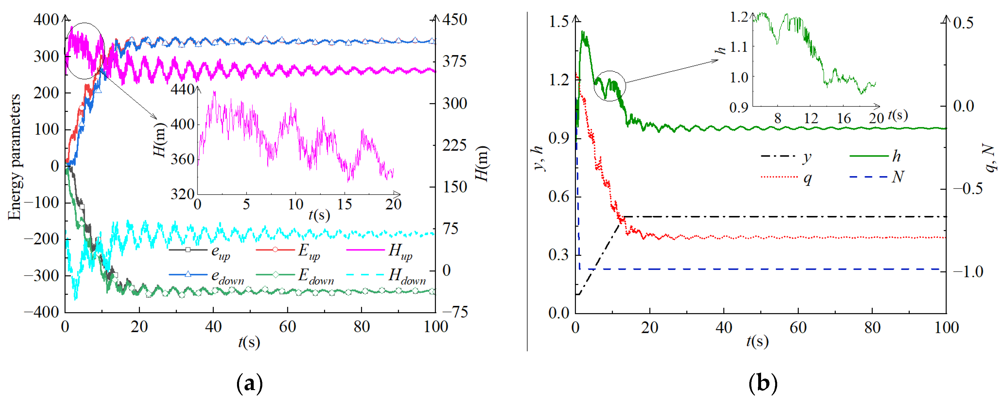
4.3. Calculation and Analysis of Pumping Conditions

As shown in Figure 21a, the energy transfer parameters on the upstream side of the unit before t = 20 s exhibit small fluctuations (−4.03 to −13.46 for E_up and 0.75 to 13.04 for e_up). At t = 30 s, the vector sum of E_up and e_up < 0 represents a negative water hammer. E_up < 0 signifies a buck wave, and the boost wave (e_up > 0) appears after reflection of E_up. At t = 49.9 s, E_up peaks while e_up is still rising, resulting in a gradual increase in their sum and the pressure. e_up reaches its maximum value at t = 50.8 s, while the pressure also reaches the maximum after 1.44 s. PC1 and PC0 share some similarities, such as the evolution trends of E_up and e_up, which exhibit small fluctuations after their peaks (−306.91 to −337.32 for E_up and 307.96 to 336.88 for e_up). The pressure fluctuation range is 341.7 m to 439.8 m. Finally, the vector sum of E_up and e_up equals 0. The energy transfer parameters on the downstream side at PC1 show the opposite circumstance compared with that of the upstream side, as listed in

Table 11. Energy transfer parameters near the upstream and downstream sides at PC1.

PC1	Emax	emax	Hest (m)	T (s)
Upstream side	−370.59	370.05	311.73	44.97
Downstream side	369.64	−370.45	159.29	42.63

. Comparing the shutdown periods of PC1 and TC3, E_max and e_max have opposite signs.

Figure 21 shows two stages at PC1. In the first stage, without guide vane movement before t = 20 s, parameters like flow remain essentially unchanged. The guide vane closure law is y = 0.5 − 0.01t in the second stage after t = 20 s, leading to a decrease in flow as the guide vane closes, while the rotation speed remains unchanged. The guide vane opening is 30% y₀ at t = 40 s, and the power supply is cut off at this moment. Reflux appears at t = 46.8 s, reaching a maximum of q_max = 0.28. The main flow takes about 52 s to stabilize at q = 0.17. The rotation speed drops to 0 at t = 79.4, after which the reverse flow causes the unit to start rotating in the opposite direction, with a final reverse speed of around N = 0.48. The pressure experiences a downward wave (h_min = 0.55, h_max = 1.27), taking 80 s to stabilize at h = 1.04. PC0 and PC1 are shutdown transitions under pumping mode, differing in guide vane closure time and power outage time. These differences are reflected in results such as the extreme values of pressure (with h_min and h_max at PC1 being 1.06 and 0.94 times those at PC0) and the extreme values of E_up and e_up around ±365 and ±355 at PC0. From the viewpoint of time, the pressure and energy transfer parameters reach their maximum values at PC0 about 40 s earlier than at PC1, due to faster guide vane closure at PC0.

As Figure 22a shows, on the upstream side of the unit, the vector sum of E_up and e_up > 0 represents a positive water hammer. E_up > 0, and the H_up rises to 143% of its original value. e_up < 0 appears after the reflection from E_up, continuing to rise even though E_up peaks at t = 18.1 s. Their vector sum decreases along with lower pressure. Lastly, the sum of E_up and e_up returns to 0, indicating the system has reached a new stable state.

Table 12. Energy transfer parameters near the upstream and downstream sides at PC2.

PC2	Emax	emax	Hest (m)	T (s)
Upstream side	348.77	−348.17	438.58	1.83
Downstream side	−344.34	344.12	−50.14	2.58

provides information on energy transfer parameters near the downstream side at PC2.

Figure 22b shows a sharp rise in rotation speed due to motor connection at PC2, with the rotation speed reaching N = 1 within 1 s. The pressure quickly reaches its maximum (h_max = 1.43 at t = 1.8 s) after the unit is powered on. h and H_up show similar trends, with a small fluctuation at t = 8 s. h declines as the guide vanes are further opened, stabilizing at h = 0.96 after 55 s. The maximum flow is q_max = −0.8 at t = 23.4 s.

4.4. Stability Analysis of Parameters (Pressure, Flow Rate, and Rotating Speed)

MDS is used to quantitatively analyze the parameters from transient conditions in Table 5. u, u₁, and u₂ are defined by Equations (25)–(27). In these expressions, c_max, c_min, and c_r are the maximum, minimum, and rated values of q, h, and N, respectively.

Table 13. u₁, u₂, and u of PSP conditions.

Conditions	q			h			N
	u1	u2	u	u1	u2	u	u1	u2	u
TC0	0.64	0.11	0.587	0.57	0.09	0.498	0.47	0.07	0.418
TC1	0.39	0.03	0.345	0.08	0.02	0.071	0.00	0.00	0.000
TC2	0.36	0.03	0.327	0.11	0.02	0.097	0.00	0.00	0.000
TC3	0.39	0.06	0.357	0.30	0.03	0.260	0.23	0.01	0.201
TC4	0.38	0.01	0.343	0.17	0.07	0.155	0.42	0.03	0.369
PC0	0.50	0.10	0.460	0.39	0.06	0.341	0.29	0.01	0.254
PC1	0.49	0.04	0.445	0.37	0.03	0.319	0.24	0.01	0.210
PC2	0.49	0.04	0.445	0.24	0.04	0.210	0.50	0.20	0.461

lists the calculated results of u₁, u₂, and u under the transitions in Table 4.

The u₁ of q follows the order TC0 > PC0 > PC1 = PC2 > TC3 = TC1 > TC4 > TC2. Comparing the startup and shutdown conditions of two modes, u₁ of PC1 and PC2 are approximately 25% larger than that of TC3 and TC4, mainly due to more obvious reflux in pumping mode. h, N, and q have similar tendencies in these four conditions, with the pumping mode exhibiting a wider fluctuation range of parameters. The u₂ of h at TC3 and TC4 is larger than that of PC1 and PC2, whereas the u₂ of q and N differ from that of h. The u₂ of q and N are larger at PC2 than at TC4, but they are greater than or equal to PC1 in TC3.

Under generation conditions in Table 5, the parameters of TC0 have the highest u₁, with the maximum and minimum u₁ of q and h differing by factors of about 2 and 7 times, respectively. The maximum and minimum u₁ of N are 0.47 and 0. As for pumping states in Table 5, the u₁ of q and h at PC0 obtain maximum values, whereas the u₁ of N reaches the maximum at PC2. The change pattern of u₂ is similar to u₁, illustrating the consistency of the two prediction results of system safety. u of N in two startup conditions (PC2 and TC4) are the largest, followed by u of q and h. However, u of q in other conditions is larger than u of h, with the smallest being u of N. A comprehensive parameter $\overline{u}$ is defined as the weighted average of q, h, and N in Equation (29).

$$\overline{u}={\displaystyle \frac{{\overline{u}}_q}{c}}+{\displaystyle \frac{{\overline{u}}_h}{c}}+{\displaystyle \frac{{\overline{u}}_N}{c}}$$

(29)

${\overline{u}}_q$, ${\overline{u}}_h$, and ${\overline{u}}_N$ are the average values of u from q, h, and N, respectively. $c={\overline{u}}_q+{\overline{u}}_h+{\overline{u}}_N$, and the calculated results of these parameters are presented in

Table 14. The weighted values of q, h, and N.

Conditions	${\overline{\mathit{u}}}_{\mathit{q}}/\mathit{c}$	${\overline{\mathit{u}}}_{\mathit{h}}/\mathit{c}$	${\overline{\mathit{u}}}_{\mathit{N}}/\mathit{c}$	$\overline{\mathit{u}}$
TC0	0.27	0.13	0.11	0.51
TC1	0.16	0.02	0.00	0.18
TC2	0.15	0.03	0.00	0.18
TC3	0.16	0.07	0.05	0.28
TC4	0.16	0.04	0.10	0.30
PC0	0.21	0.09	0.07	0.37
PC1	0.20	0.09	0.06	0.35
PC2	0.20	0.06	0.12	0.38

. The order of condition safety is TC2 = TC1 > TC3 > TC4 > PC1 > PC0 > PC2 > TC0. TC1 and TC2 exhibit the best safety, whereas TC0 shows the worst case, with the $\overline{u}$ of TC0 being approximately 2.5 times that of TC1 and TC2.

5. Conclusions

This work proposes a method called WHED used for guarantee calculation of regulation for HPs and PSPs. The WHED calculation results for HPs show good agreement with experimental data, demonstrating WHED’s reliability. Furthermore, WHED and MOC are used to analyze the generating and pumping modes of PSPs, with results revealing WHED’s superiority over MOC. Energy parameters are defined to characterize the operational stability of transitions, while MSD is applied to explore the stability of transient parameters.

The key findings of this study include the following three aspects.

(1)

A key contribution of this paper is the proposal of WHED: WHED employs energy transfer parameters to characterize system stability, which makes it possible to explain the operations of HPs and PSPs from a physical point of view, and it further breaks the limitation of MOC being limited to mathematical analyses. Thus WHED does not need to take into account the Courant condition in its calculation. Also, WHED can be used with a large time step condition so that it can directly calculate the transient parameters of the target node, improving calculation speed by about 4 times compared with MOC.

(2)

The behavior of core parameters in WHED: Negative energy waves are always reflected from positive energy waves, meaning that the negative energy transfer parameter appears later than the positive energy transfer parameter. The energy transfer parameter reflects the energy variation in the system, and the pattern of energy transfer on the upstream side is opposite to that on the downstream side. The regulating well can effectively reduce water hammer pressure, so the energy transfer parameter in the regulating well changes in the opposite direction to that in the pipeline. Larger load adjustments correspond to greater changes in energy transfer parameters and increased system instability. The positive and negative values of the energy transfer parameters indicate different types of water hammer, with positive values corresponding to positive water hammer as pressure increases. The system is stable when the sum of the positive and negative energy transfer parameters equals zero.

(3)

This paper verifies the accuracy of WHED by comparing it with model tests and MOC. Due to limitations of the test bench, the wave speed used in the model experiment differs from that in the calculation, resulting in a larger discrepancy in the model test compared to the calculation verification. The smallest error occurs in the TC0 condition, demonstrating that the water hammer energy difference calculation method is highly reliable based on the comparison of results. Additionally, the one-dimensional and three-dimensional coupled calculations highlight the broad applicability of WHED in scientific research. The coupling performance is well validated through comparison with experimental results, and CFD simulations of TKE distribution in the regulating well show that turbulence is more intense in the low-water-level transition condition.

Stable operation of transitions in the regulated plants can effectively reduce wind and solar abandonment rates and enhance their power acceptance capacity, and it further contributes to the construction of new energy power grids. WHED’s application to investigate transient characteristics of more PSPs and HPs and analyze the impact of unstable transitions on the grid will be the next study for the authors.

References

1. Liu, X.; Ni, Y.; Sun, Y.; Wang, J.; Wang, R.; Sun, Q. Multi-VPPs power-carbon joint trading optimization considering low-carbon operation mode. J. Energy Storage 2024, 83, 110786. [Google Scholar]
2. Ma, X.; Zhai, Y.; Zhang, T.; Yao, X.; Hong, J. What changes can solar and wind power bring to the electrification of China compared with coal electricity: From a cost-oriented life cycle impact perspective. Energy Convers. Manag. 2023, 289, 117162. [Google Scholar] [CrossRef]
3. Morabito, A.; Hendrick, P. Pump as turbine applied to micro energy storage and smart water grids: A case study. Appl. Energy 2019, 241, 567–597. [Google Scholar]
4. Ali, M.; Ahmad, M.; Koondhar, M.A.; Akram, M.S.; Verma, A.; Khan, B. Maximum power point tracking for grid-connected photovoltaic system using adaptive fuzzy logic controller. Comput. Electr. Eng. 2023, 110, 108879. [Google Scholar] [CrossRef]
5. Oskouei, M.Z.; Yazdankhah, A.S. Scenario-based stochastic optimal operation of wind, photovoltaic, pump-storage hybrid system in frequency-based pricing. Energy Convers. Manag. 2015, 105, 1105–1114. [Google Scholar] [CrossRef]
6. Fang, G.; Chen, G.; Yang, K.; Yin, W.; Tian, L. How does green fiscal expenditure promote green total factor energy efficiency?-Evidence from Chinese 254 cities. Appl. Energy 2024, 353, 122098. [Google Scholar] [CrossRef]
7. Luo, X.Q.; Zhu, G.J.; Feng, J.J. The technology progress and development trend of hydraulic turbine. J. Hydroelectr. Eng. 2020, 39, 1–18. (In Chinese) [Google Scholar]
8. Chen, Y.; Deng, C.; Wu, H.; Li, D.; Chen, M.; Peng, P.; Zhao, Y. Multi-stage Soft Coordinated Control of Variable Speed Pumped Storage Unit in the Process of Mode Conversion Under the Generation Condition. Proc. CSEE 2021, 41, 5258–5274. (In Chinese) [Google Scholar]
9. Hu, J.; Yang, J.; He, X.; Zhao, Z.; Yang, J. Transient analysis of a hydropower plant with a super-long headrace tunnel during load acceptance: Instability mechanism and measurement verification. Energy 2023, 263, 125671. [Google Scholar] [CrossRef]
10. Zhao, H.J.; Liu, S.B.; Zhang, Y.H. Study on reservoir ice regime of Pushihe pumped-storage power station. Water Power 2019, 45, 90–94. (In Chinese) [Google Scholar]
11. Yuan, B.; Li, C.; Feng, Y. Partition of operating regions in turbine mode for No.4 unit of Pushihe pumped storage power station. Water Resour. Power 2017, 35, 153–157. (In Chinese) [Google Scholar]
12. Lu, J.; Wu, G.; Zhou, L.; Wu, J. Finite Volume method for modeling the load-rejection process of a hydropower plant with an air cushion surge chamber. Water 2023, 15, 682. [Google Scholar] [CrossRef]
13. Ma, Z.; Zhu, B. Pressure fluctuations in vaneless space of pump-turbines with large blade lean runners in the S-shaped region. Renew. Energy 2020, 153, 1283–1295. [Google Scholar] [CrossRef]
14. Nasir, J.; Javed, A.; Ali, M.; Ullah, K.; Kazmi, S.A.A. Capacity optimization of pumped storage hydropower and its impact on an integrated conventional hydropower plant operation. Appl. Energy 2022, 323, 119651. [Google Scholar] [CrossRef]
15. Yang, Z.; Liu, Z.; Cheng, Y.; Zhang, X.; Liu, K.; Xia, L. Differences of Flow Patterns and Pressure Pulsations in Four Prototype Pump-Turbines during Runaway Transient Processes. Energies 2020, 13, 5296. [Google Scholar] [CrossRef]
16. Li, Z.; Bi, H.; Karney, B.; Wang, Z.; Yao, Z. Three-dimensional transient simulation of a prototype pump-turbine during normal turbine shutdown. J. Hydraul. Res. 2017, 55, 520–537. [Google Scholar] [CrossRef]
17. Su, W.-T.; Li, X.-B.; Xia, Y.-X.; Liu, Q.-Z.; Binama, M.; Zhang, Y.-N. Pressure fluctuation characteristics of a model pump-turbine during runaway transient. Renew. Energy 2021, 163, 517–529. [Google Scholar] [CrossRef]
18. Henclik, S. Analytical solution and numerical study on water hammer in a pipeline closed with an elastically attached valve. J. Sound Vib. 2018, 417, 245–259. [Google Scholar] [CrossRef]
19. Urbanowicz, K.; Bergant, A.; Stosiak, M.; Deptuła, A.; Karpenko, M.; Kubrak, M.; Kodura, A. Water Hammer Simulation Using Simplified Convolution-Based Unsteady Friction Model. Water 2022, 14, 3151. [Google Scholar] [CrossRef]
20. Yang, Z.; Cheng, Y.; Xia, L.; Meng, W.; Liu, K.; Zhang, X. Evolutions of flow patterns and pressure fluctuations in a prototype pump-turbine during the runaway transient process after pump-trip. Renew. Energy 2020, 152, 149–1159. [Google Scholar] [CrossRef]
21. Hou, J.; Li, G.H.; Li, X.X.; Wu, X.M.; Chen, Y.M. Transient Process of Complex Hydraulic System; China & Water Power Press: Beijing, China, 2019. (In Chinese) [Google Scholar]
22. Zhang, L.; Wu, Q.; Ma, Z.; Wang, X. Transient vibration analysis of unit-plant structure for hydropower station in sudden load increasing process. Mech. Syst. Signal Process. 2019, 120, 486–504. [Google Scholar] [CrossRef]
23. Telikani, A.; Rossi, M.; Khajehali, N.; Renzi, M. Pumps-as-Turbines (PaTs) performance prediction improvement using evolutionary artificial neural networks. Appl. Energy 2023, 330, 120316. [Google Scholar] [CrossRef]
24. Zhang, Y.; Xu, Y.; Zheng, Y.; Rodriguez, E.F.; Liu, H.; Feng, J. Analysis on Guide Vane Closure Schemes of High-Head Pumped Storage Unit during Pump Outage Condition. Math. Probl. Eng. 2019, 2019, 8262074. [Google Scholar] [CrossRef]
25. Yu, X.; Zhang, J.; Zhou, L. Hydraulic Transients in the Long Diversion-Type Hydropower Station with a Complex Differential Surge Tank. Sci. World J. 2014, 2014, 241868. [Google Scholar] [CrossRef] [PubMed]
26. Li, H.; Wan, Z.; Huang, W.; Zeng, M.; Fang, J.; Xie, J. Robust comprehensive evaluation of guide vane closure law in hydraulic turbines in moderately-high head hydropower plants. J. Tsinghua Univ. (Sci. Technol.) 2023, 63, 125–133. (In Chinese) [Google Scholar]
27. Wang, Y.; Zhang, J.; Xu, T.; Liu, Y.; Yao, T.; Wang, K.; Zhang, M. Air valve arrangement criteria for preventing secondary pipe bursts in long-distance gravitational water supply systems. Aqua-Water Infrastruct. Ecosyst. Soc. 2023, 72, 1566–1581. [Google Scholar] [CrossRef]
28. Trivedi, C.; Gandhi, B.K.; Cervantes, M.J.; Dahlhaug, O.G. Experimental investigations of a model Francis turbine during shutdown at synchronous speed. Renew. Energy 2015, 83, 828–836. [Google Scholar] [CrossRef]
29. Ye, J.; Do, N.C.; Zeng, W.; Lambert, M. Physics-informed neural networks for hydraulic transient analysis in pipeline systems. Water Res. 2022, 211, 118828. [Google Scholar] [CrossRef]
30. Chen, S.; Wang, J.; Zhang, J.; Yu, X.; He, W. Transient behavior of two-stage load rejection for multiple units system in pumped storage plants. Renew. Energy 2020, 169, 1012–1022. [Google Scholar] [CrossRef]
31. Mao, X.; Zhong, P.; Wang, Y.; Tan, Q.; Cui, Q. Study on the evolution of transient flow field in WDS based on numerical and experimental methods. J. Energy Storage 2023, 73, 108996. [Google Scholar] [CrossRef]
32. Zhang, W.; Deng, J.; Wang, P.; Wang, Y. Study on similitude method for turbine considering working fluid physical properties variation. Appl. Energy 2023, 338, 120930. [Google Scholar] [CrossRef]
33. Zhang, P.; Cheng, Y.; Xue, S.; Hu, Z.; Tang, M.; Chen, X. 1D-3D coupled simulation method of hydraulic transients in ultra-long hydraulic systems based on OpenFOAM. Eng. Appl. Comput. Fluid Mech. 2023, 17, 2229889. [Google Scholar] [CrossRef]
34. Bi, H.; Chen, F.; Wang, C.; Wang, Z.; Fan, H.; Luo, Y. Analysis of dynamic performance in a pump-turbine during the successive load rejection. IOP Conf. Ser. Earth Environ. Sci. 2021, 774, 012152. [Google Scholar] [CrossRef]
35. Cherny, S.; Chirkov, D.; Bannikov, D.; Lapin, V.; Skorospelov, V.; Eshkunova, I.; Avdushenko, A. 3D numerical simulation of transient processes in hydraulic turbines. IOP Conf. Ser. Earth Environ. Sci. 2010, 12, 012071. [Google Scholar] [CrossRef]
36. Zhang, X.-X.; Cheng, Y.-G.; Yang, J.-D.; Xia, L.-S.; Lai, X. Simulation of the load rejection transient process of a francis turbine by using a 1D-3D coupling approach. J. Hydrodyn. 2014, 26, 715–724. [Google Scholar] [CrossRef]
37. Cheng, Y.C.; Zhang, J.B.; Chen, G.; Zhang, D. Automatic Regulation of Water Turbine; China Water & Power Press: Beijing, China, 2010. (In Chinese) [Google Scholar]
38. Zheng, Y.; Zhang, J. Hydro Unit Transition Process; Peking University Press: Beijing, China, 2008. (In Chinese) [Google Scholar]
39. Mao, X.L.; Wen, G.Q. Pumped Storage Power Station Power Generation Mode Full Load Condition and Pumping Mode Power Off Condition Transition Process Calculation Software, version 2023SR1542053; Northwest A & F University: Xianyang, China, 2023. (In Chinese)
Figure 1. PSP cooperates with power generation by clean energy.
Energies 18 01549 g001
Figure 2. Propagation of pressure wave in pipeline.
Energies 18 01549 g002
Figure 3. Parameters of transfer energy in pipeline with varying diameter and bifurcated conduit. (a) A pipe with different diameters; (b) Bifurcated conduit.
Energies 18 01549 g003
Figure 4. The information of experiment. (a) The layout of test bench; (b) Flow control laws.
Energies 18 01549 g004
Figure 5. Schematic diagram of HP. (The triangle in the figure represents the water level line, 1–11 represents the pipeline number, and the parameters are shown in Table 1).
Energies 18 01549 g005
Figure 6. The flow charts of calculation in HP. (a) Application steps of WHED; (b) The calculation process of transient conditions.
Energies 18 01549 g006
Figure 7. WHED and experiment results at ET1. (a) Pressure of H1, H2, and H3; (b) Pressure of HW and HB; (c) Energy transfer parameters.
Energies 18 01549 g007
Figure 8. WHED and experiment results at ET2. (a) Pressure of H1, H2, and H3; (b) Pressure of HW and HB; (c) Energy transfer parameters.
Energies 18 01549 g008
Figure 9. WHED and experiment results at ET3. (a) Pressure of H1, H2, and H3; (b) Pressure of HW and HB; (c) Energy transfer parameters.
Energies 18 01549 g009
Figure 10. WHED and experiment results at ET4. (a) Pressure of H1, H2, and H3; (b) Pressure of HW and HB; (c) Energy transfer parameters.
Energies 18 01549 g010
Figure 11. The 1D WHED coupling 3D numerical simulation. (a) Grid-independence validation; (b) Coupling performance validation.
Energies 18 01549 g011
Figure 12. TKE distribution in regulating well under 4 experimental conditions. (a) ET1; (b) ET2; (c) ET3; (d) ET4.
Energies 18 01549 g012
Figure 13. Layout of one PSP in China.
Energies 18 01549 g013
Figure 14. The complete characteristic curves of pump turbine. (a) n11-Q11; (b) x-WH; (c) n11-M11; (d) x-WM.
Energies 18 01549 g014
Figure 15. The results of TC0 condition. (a) Rotation speed, flow, and pressure; (b) Energy transfer parameters.
Energies 18 01549 g015
Figure 16. The results of PC0 condition. (a) Rotation speed, flow, and pressure; (b) Energy transfer parameters.
Energies 18 01549 g016
Figure 17. Calculation results of TC1 condition. (a) Energy transfer parameters; (b) Rotation speed, flow, and pressure.
Energies 18 01549 g017
Figure 18. Calculation results of TC2 condition. (a) Energy transfer parameters; (b) Rotation speed, flow, and pressure.
Energies 18 01549 g018
Figure 19. Calculation results of TC3 condition. (a) Energy transfer parameters; (b) Rotation speed, flow, and pressure.
Energies 18 01549 g019
Figure 20. Calculation results of TC4 condition. (a) Energy transfer parameters; (b) Rotation speed, flow, and pressure.
Energies 18 01549 g020
Figure 21. Calculation results of PC1 condition. (a) Energy transfer parameters; (b) Rotation speed, flow, and pressure.
Energies 18 01549 g021
Figure 22. Calculation results of PC2 condition. (a) Energy transfer parameters; (b) Rotation speed, flow, and pressure.
Energies 18 01549 g022