Research on Diagnostic Methods for Zero-Value Insulators in 110 kV Transmission Lines Based on Spatial Distribution Characteristics of Electric Fields

Abstract

Porcelain insulators in power systems are subject to prolonged mechanical and electrical loads, as well as environmental factors such as climate variations. These conditions often lead to degradation of insulation performance and structural damage, resulting in a decrease in insulation resistance and the formation of cracks, which in turn produce “zero-value” insulators. The presence of zero-value insulators significantly increases the risk of pollution flashovers and electrical arcing, with flashover occurrences possible even under normal operating voltages. This poses a severe threat to the safe and stable operation of the power grid. This study develops a high-fidelity simulation model of insulator strings containing zero-value defects for a 110 kV transmission line. The impact of variations in the position and quantity of zero-value insulators on the spatial electric field distribution is analyzed in detail. Based on the electric field changes, a detection method for zero-value insulators is proposed. Additionally, a prediction model for the electric field strength of insulators with zero-value defects is developed using a Multilayer Perceptron (MLP) neural network. A spatial electric field distribution database for insulator strings containing zero-value defects is also established. The accuracy of the model is validated through laboratory testing.

1. Introduction

The insulator, as a core component of overhead transmission lines, is essential for the stable and safe operation of the power grid [1,2]. Porcelain insulators, known for their superior insulating properties, are susceptible to internal degradation when exposed over time to complex environmental conditions and high voltages. This degradation, affecting the adhesive within the porcelain, leads to a continuous decrease in internal resistance, eventually resulting in zero-value insulators [3,4]. In overhead lines, the presence of zero-value insulators significantly increases the risk of insulator string breakage or detachment, posing a serious threat to grid stability. Therefore, monitoring the condition of insulators is of critical importance to ensure grid safety [5,6,7].

Traditional insulator inspection methods, such as insulation resistance testing and spark gap testing, involve high-risk, contact-based procedures requiring personnel to ascend transmission towers. These methods are labor-intensive and time-consuming, and the insulation resistance method requires a power outage [8]. In light of these challenges, researchers have explored non-contact methods, including ultraviolet and infrared imaging. However, these techniques are often vulnerable to environmental interference, leading to potential issues of missed or false detections [9,10,11]. To enhance the efficiency of zero-value detection, the electric field distribution method has emerged as a promising alternative. This approach leverages the spatial electric field characteristics of insulators to enable non-contact inspection. It offers greater immunity to environmental factors, lower detection costs, and yields relatively accurate measurements.

Research has been conducted on insulator degradation detection based on the electric field distribution method. M. Ramesh et al. used an electro-optic probe based on the Pockels effect to measure electric fields, demonstrating differences between defective and healthy insulators [12]. Yangchun Cheng et al. proposed a novel live detection method for zero-value insulators and verified experimentally that the location of zero-value insulators could be identified by changes in the electric field distribution curve [13]. Yi Xu et al. developed a detection device based on electric field distribution principles; however, the device requires scanning the entire insulator string’s field distribution curve, resulting in low detection efficiency [14]. To improve detection efficiency, Dongdong Zhang et al. introduced an innovative focus on local electric field detection, demonstrating its effectiveness in identifying zero-value insulators through simulation, opening a new pathway for improving detection efficiency in transmission lines [15].

Currently, the majority of research is confined to purely simulation analyses, lacking essential experimental validation, and thus fails to offer definitive guidance on the optimal detection distance in field inspections. Furthermore, there exists a significant data deficiency concerning the spatial electric field distribution characteristics of porcelain insulator strings. To address these issues, this study employed finite element simulation techniques to investigate the detection of degraded insulators. A testing platform for degraded insulator detection was developed, and the effects of detection distance, the position of zero-value insulators, and their quantity on the electric field distribution of insulator strings were systematically analyzed. The distribution patterns of electric field intensity under various zero-defect conditions in insulator strings were subsequently revealed. Furthermore, a multi-layer perceptron (MLP) neural network model was utilized to construct a spatial electric field distribution dataset for insulator strings with zero-value defects, leading to the establishment of a corresponding database. The findings of this study provide robust theoretical and data support for field detection of zero-value insulators based on the electric field method.

2. Simulation Model of Suspension Insulator Strings

In this section, a 1:1 three-dimensional electric field simulation model of a tower-insulator string was established using Comsol 6.2 finite element simulation software. Based on electrostatic principles, a method for calculating the electric field distribution within the insulator string and its surrounding space was proposed, along with boundary conditions for the entire electric field simulation model.

2.1. Model Development

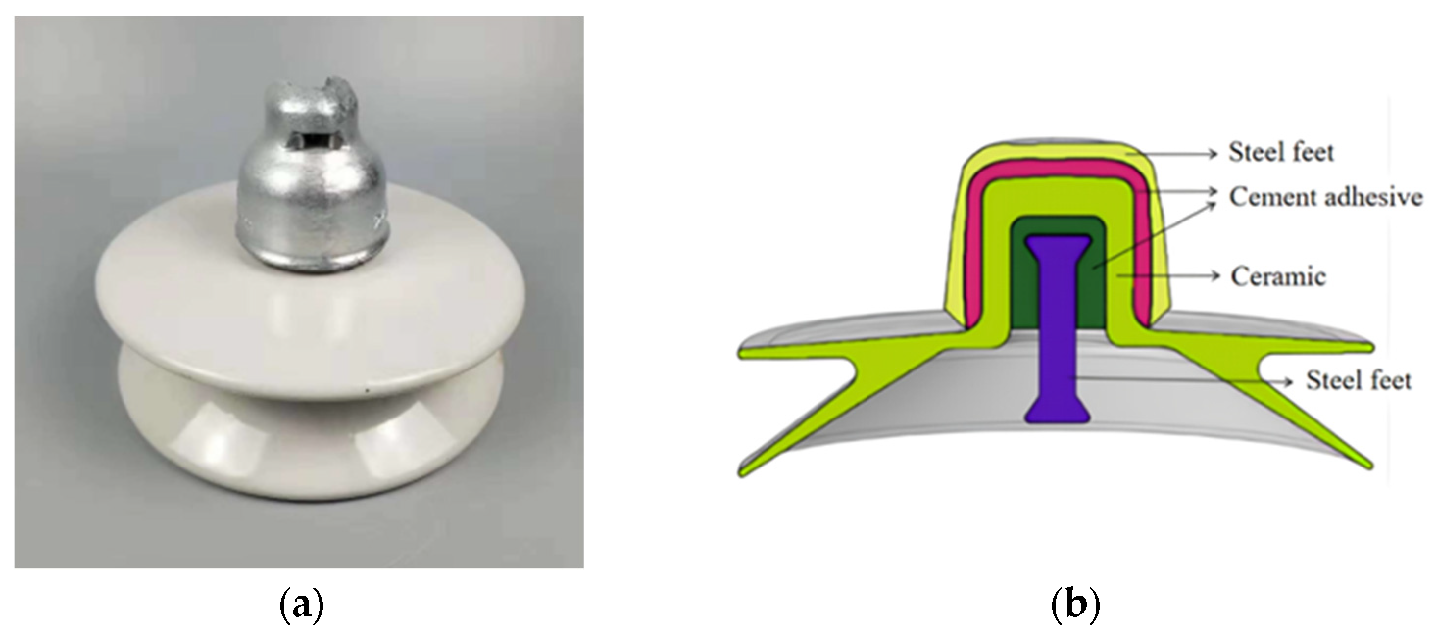
The U70BP-160 porcelain insulator (Dalian Insulator Group T&D Co., Ltd. Dalian, China) was selected as the study object, and a 3D simulation model was created in Comsol, as shown in Figure 1b. The model includes key components: the ceramic steel feet, steel cap, and cement adhesive. The porcelain insulator has a height of 146 mm and a diameter of 280 mm, with the steel cap’s maximum diameter being 100 mm.

For zero-value insulators, the primary areas of degradation are at the connections among the steel cap, porcelain body, and steel feet. In this model, through-connections between the steel cap, porcelain, and cement adhesive were created, and the entire through-region was set as a conductive metal material to simulate a zero-value defect. The relative permittivity of the defect area is configured to be at least 1000 times that of the surrounding non-metal conductors.

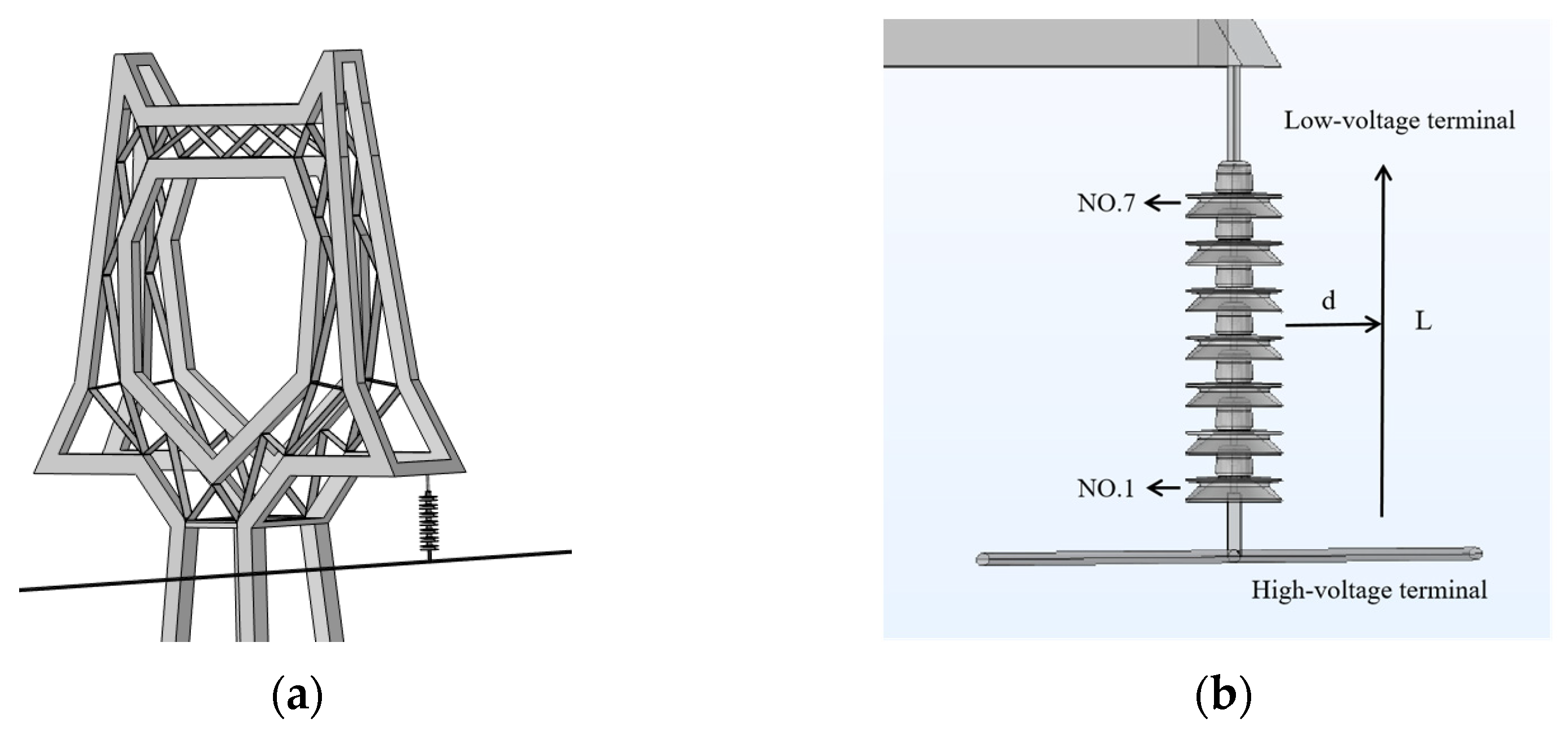
As shown in Figure 2, the model includes the tower, insulator string, upper and lower fittings, conductor, and an air domain surrounding the insulator string. The electrical configuration comprised a seven-unit U70BP-160 porcelain insulator string. A 20-m conductor assembly with surrounding air domains (radially extending 5 m from the insulator string) was computationally modeled to characterize the spatial electric field distribution. Figure 3 shows the porcelain insulator string model, composed of seven identical insulators numbered from 1 to 7 from bottom to top, where Insulator 1 is connected to the conductor and Insulator 7 is connected to the tower. The parameter d represents the distance from various measurement points to the outer edge of the insulator string, with the electric field detection path along the straight line L, defined as the axial direction in space. Internal component dimensions and material properties were specified, and each part of the insulator was populated with corresponding materials.

An electrostatic analysis approach was applied for simulation calculations, with primary material parameters outlined in

Table 1. Key material parameters for electric field calculation.

Materials	Relative Permittivity
Steel Cap, Steel Foot	1 × 108
Cement Binder	14
Ceramic Components	6
Conductor	1000
Pole Tower	2000
Fittings	1000

. The electric field simulation employs electrostatic field boundary conditions, where an AC phase voltage of 63.5 kV is applied to the high-voltage end of the insulator string (conductor, connecting hardware, and steel foot of the first insulator). The tower, the steel cap of the last insulator, and the connecting hardware are grounded, with the air domain enforced at 0 potential.

2.2. Finite Element Calculation Method and Boundary Condition Setup

In the three-dimensional electrostatic field model presented in this paper [16], the potentials of the tower, conductor, and insulator satisfy Poisson’s equation based on the principles of electrostatics, as shown in Equation (1).

$${\nabla }^2\phi ={\displaystyle \frac{{\partial }^2\phi }{\partial {\mathrm{x}}^2}}+{\displaystyle \frac{{\partial }^2\phi }{\partial y^2}}+{\displaystyle \frac{{\partial }^2\phi }{\partial z^2}}=-{\displaystyle \frac{\rho }{\epsilon }}$$

(1)

In these equations, ∇² denotes the Laplace operator, ε represents the permittivity of the dielectric medium, ρ is the spatial charge density, and φ is the electric potential.

To obtain the electric field distribution characteristics of a ceramic insulator string, it is necessary to establish an electric field control equation specific to the insulator string. A 63.5 kV AC phase voltage is applied to the high-voltage end of the insulator string, and the electric field within and around the surrounding air is analyzed. Assuming the influence of space charges is negligible, the solution can be derived using the electrostatic field method. In the simulation model presented, the influence of space charges on the electric field simulation is neglected. Consequently, the resulting potential function Φ satisfies the following equation:

$${\nabla }^2\phi =0$$

(2)

In the simulation calculations for the test model, first-type boundary conditions are uniformly applied as follows:

$$\phi {|}_{{\Gamma }_0}=0$$

(3)

$$\phi {|}_{{\Gamma }_{\mathrm{k}}}=U_0$$

(4)

In these equations, ${\mathsf{\Gamma }}_0$ represents the boundary of the air region and the ground, while ${\mathsf{\Gamma }}_{\mathrm{k}}$ denotes the high-potential simulation model. Equations (2) through (4) collectively define the boundary conditions for the entire electric field simulation model.

3. Spatial Electric Field Distribution Characteristics of Insulator Strings Under Various Conditions

This section investigates the impact of detection distance (20 mm to 2000 mm) on the electric field distribution of a 110 kV insulator string through simulation. The effects of the position and number of zero-value insulators under different conditions (single insulators, double insulators with discontinuous zero-value defects, and double insulators with continuous zero-value defects) on the electric field intensity are also analyzed. A comparison between the zero-value defects and normal conditions reveals the specific influence of detection distance and zero-value conditions on the electric field distribution.

3.1. Effects of Detection Distance on the Spatial Electric Field of Insulator Strings

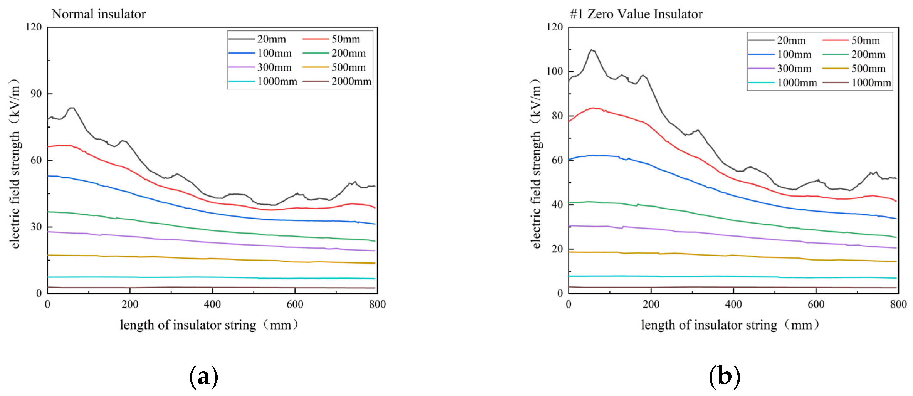
In 110 kV insulator strings, the electric potential decreases uniformly from the high-voltage end to the low-voltage end, with field intensity highest near the high-voltage end, diminishing in the middle, and slightly increasing near the low-voltage end. To investigate the effects of detection distance and zero-value defects on the spatial electric field distribution, the first insulator was set as a zero-value insulator and spatial electric field distribution simulations were conducted across a range of detection distances from 20 mm to 2000 mm. The resulting electric field intensity distribution curves are shown in Figure 3.

Analysis of Figure 3a reveals that, under normal conditions, the electric field strength increases as the detection point moves closer to the insulator string, exhibiting a “U” shaped distribution. At d = 20 mm, the field strength fluctuates due to the insulator’s shape, while at d = 2000 mm, it becomes nearly linear. Figure 3b indicates that the #1 zero-value insulator causes significant distortion, particularly at 100 mm, with the distortion effect decreasing along the string. The comparison reveals that the zero-value effect is most pronounced at 20 mm, with the response diminishing beyond 300 mm. Therefore, the detection distance should be maintained between 20 mm and 300 mm to accurately capture the electric field changes.

3.2. Effects of Zero-Value Insulator Position on the Spatial Electric Field of Insulator Strings

To investigate the effect of insulator degradation location on the surrounding field strength, simulations were conducted by varying the relative permittivity to model conditions with single, discontinuous dual, and continuous dual zero-value insulators. The electric field distribution of the insulator string was analyzed under each condition to obtain spatial electric field characteristic curves, allowing for a comparison of how different degradation locations impact field strength variation.

3.2.1. Electric Field Distribution Characteristics with a Single Zero-Value Insulator

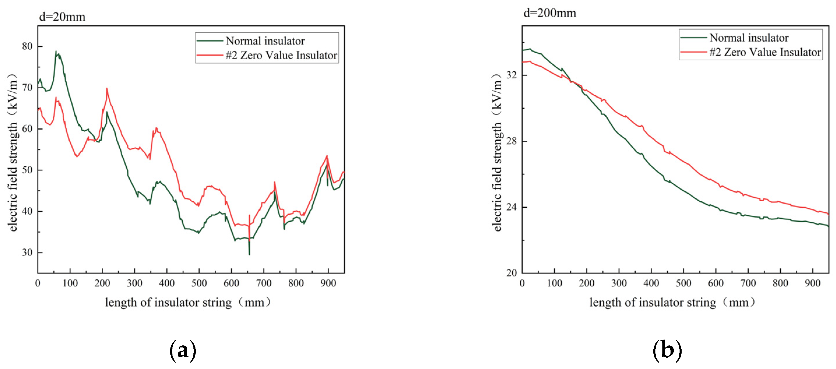
In the single insulator zero-value scenario, where the second insulator is set as zero-value, the electric field distribution at d = 20 mm and d = 200 mm is compared, as shown in Figure 4. Under normal conditions, the electric field transitions from a fluctuating shape to a smoother “U” shape as the distance increases. With the #2 zero-value insulator, the electric field is significantly distorted at that location, with a maximum distortion rate of 30% at d = 20 mm. The field decreases below the zero-value insulator and increases above it, with a smooth transition at the zero-value point, demonstrating the significant impact of the zero-value insulator on the surrounding electric field.

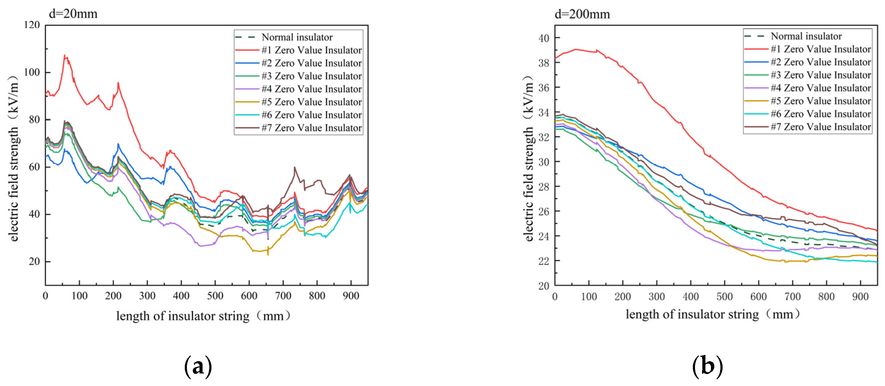
To further analyze the impact of the location of a single degraded insulator on the electric field distribution, simulations were conducted with insulators 1 through 7 set as zero-value insulators. The electric field distributions at d = 20 mm and d = 200 mm were then compared. Figure 5 compares the electric field variations under normal conditions and with zero-value insulators at different positions. Under normal conditions, the electric field decreases from the high-voltage end (No. 1) to the low-voltage end (No. 7) before increasing again. The zero-value insulators significantly affect the field distribution, especially at the high-voltage end (No. 1), where the peak electric field reaches 109.6 kV/m and the distortion rate is 50% at d = 20 mm. This study shows that the location of insulator degradation, particularly at the high-voltage and tower ends, significantly influences the electric field distribution.

3.2.2. Electric Field Distribution Characteristics with Discontinuous Double Zero-Value Insulators

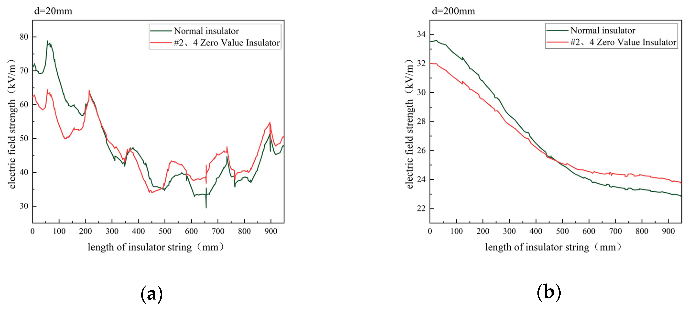
Building on the analysis of a single zero-value condition, the effect of discontinuous dual zero-value insulators (#2 and #4) on the electric field distribution outside the insulator string was further examined, as shown in Figure 6. When Insulators #2 and #4 were set as zero-value, the electric field distribution showed significant changes at both d = 20 mm and d = 200 mm. Each degraded insulator had an effect similar to that of a single zero-value unit; however, the simultaneous degradation of both insulators intensified field distortion, with a maximum distortion rate of 25% at d = 20 mm. Increased detection distance led to a reduction in overall electric field strength and a lower distortion rate, indicating that the impact of electric field distortion diminishes with distance.

3.2.3. Electric Field Distribution Characteristics with Continuous Double Zero-Value Insulators

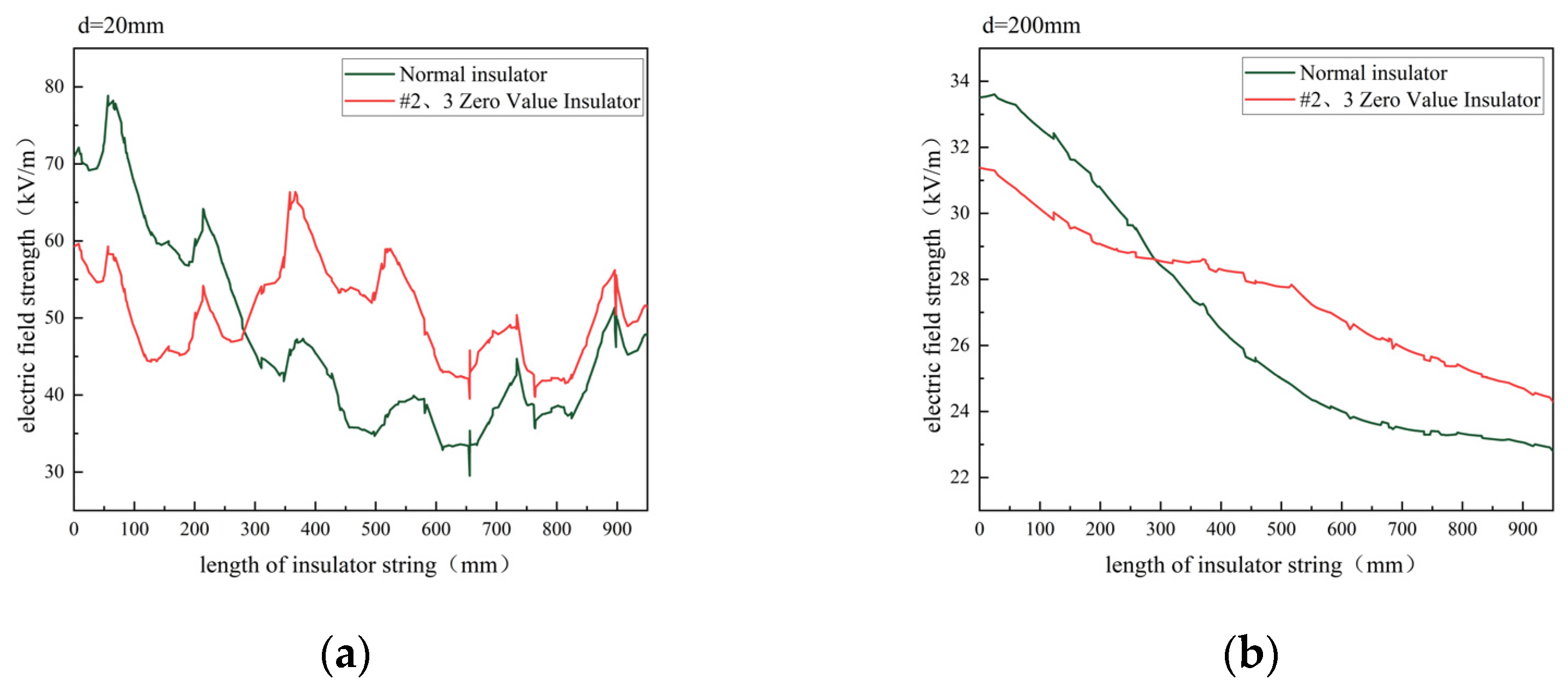
To investigate the influence of continuous dual zero-value insulators on the electric field distribution, Insulators #2 and #3 were set to zero-value, and electric field distribution measurements were taken at d = 20 mm and d = 200 mm, as depicted in Figure 7. Field strength was found to weaken below the zero-value area and strengthen above, with a smooth transition at the defect boundary. Continuous degradation caused more significant changes in the electric field than single-unit degradation, with a maximum distortion rate of 52.8% at d = 20 mm. The electric field intensity increased by approximately 20 kV/m near the third zero-value insulator compared to normal conditions.

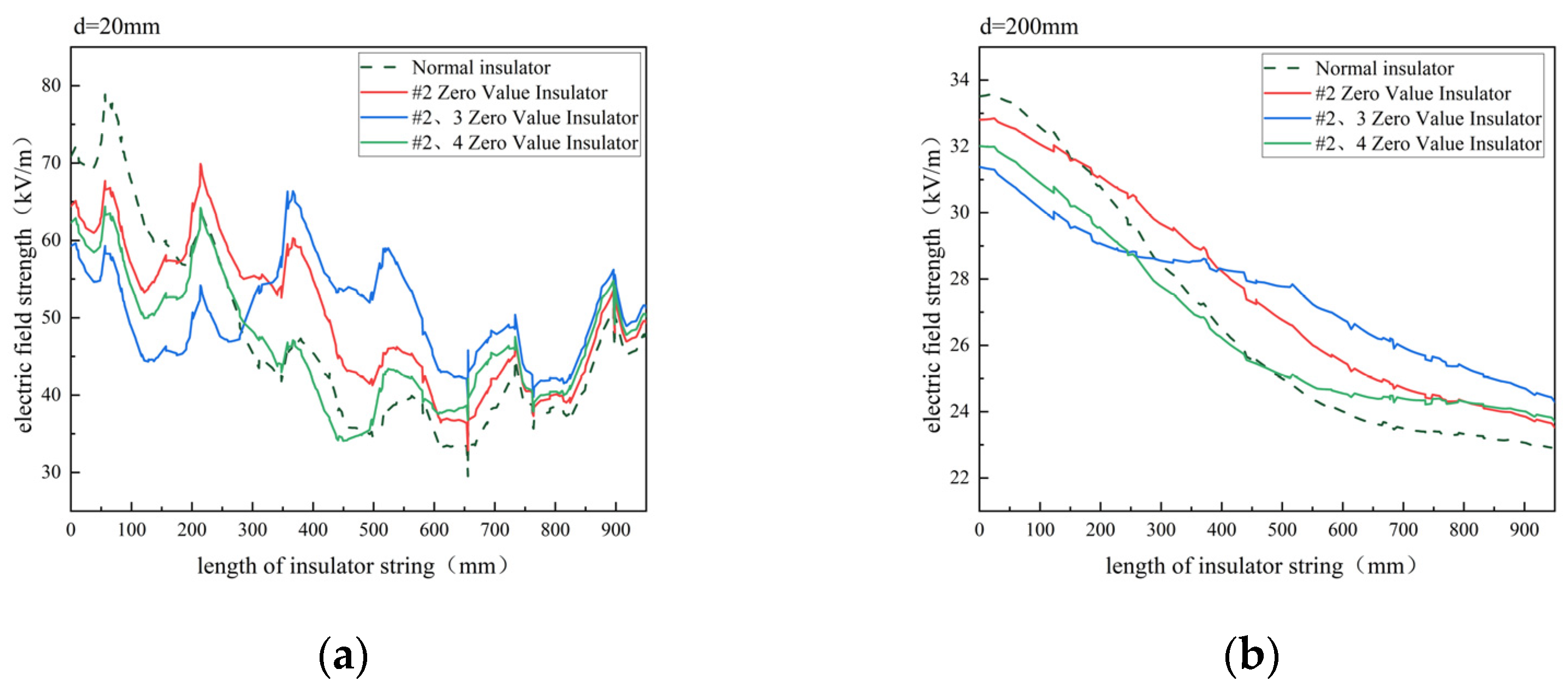
Comparative analysis of normal, single zero-value, discontinuous dual, and continuous dual degradation cases revealed that increasing detection distance reduces the impact of degraded insulators on the spatial electric field. As shown in Figure 8, degradation location significantly affects the spatial electric field, particularly at the high-voltage end and the tower connection, with less influence in the middle. The effect of continuous dual degradation on spatial electric field variation was found to be greater than that of discontinuous degradation and single-unit degradation.

4. Intelligent Prediction Algorithm for Insulator String Electric Field Based on MLP Neural Network

Simulation data can only capture the electric field distribution characteristics at specific distances, making it challenging to comprehensively reveal variations across all distances. To facilitate on-site testing and data analysis, a multi-layer perceptron (MLP) neural network model was employed to construct a spatial electric field distribution dataset for insulator strings with zero-value defects. Based on this dataset, a corresponding database was established.

4.1. Multilayer Perceptron Neural Network Model

In this study, an MLP neural network combined with four different optimization algorithms was first employed to perform linear fitting of the target, establishing a three-layer neural network model to map the nonlinear relationship between electric field intensity and influencing factors. The MLP neural network was trained using the Levenberg–Marquardt algorithm, the Bayesian regularization algorithm, and the scaled conjugate gradient algorithm. Additionally, a genetic algorithm was embedded into the neural network to achieve global optimization of weights and thresholds. Finally, the established MLP neural network models based on the four optimization algorithms were applied to perform nonlinear fitting of the mapping relationship between electric field intensity and influencing factors. The convergence speed and fitting performance of each model were compared, and the Bayesian regularization-based MLP neural network was ultimately selected as the optimal model for predicting electric field intensity.

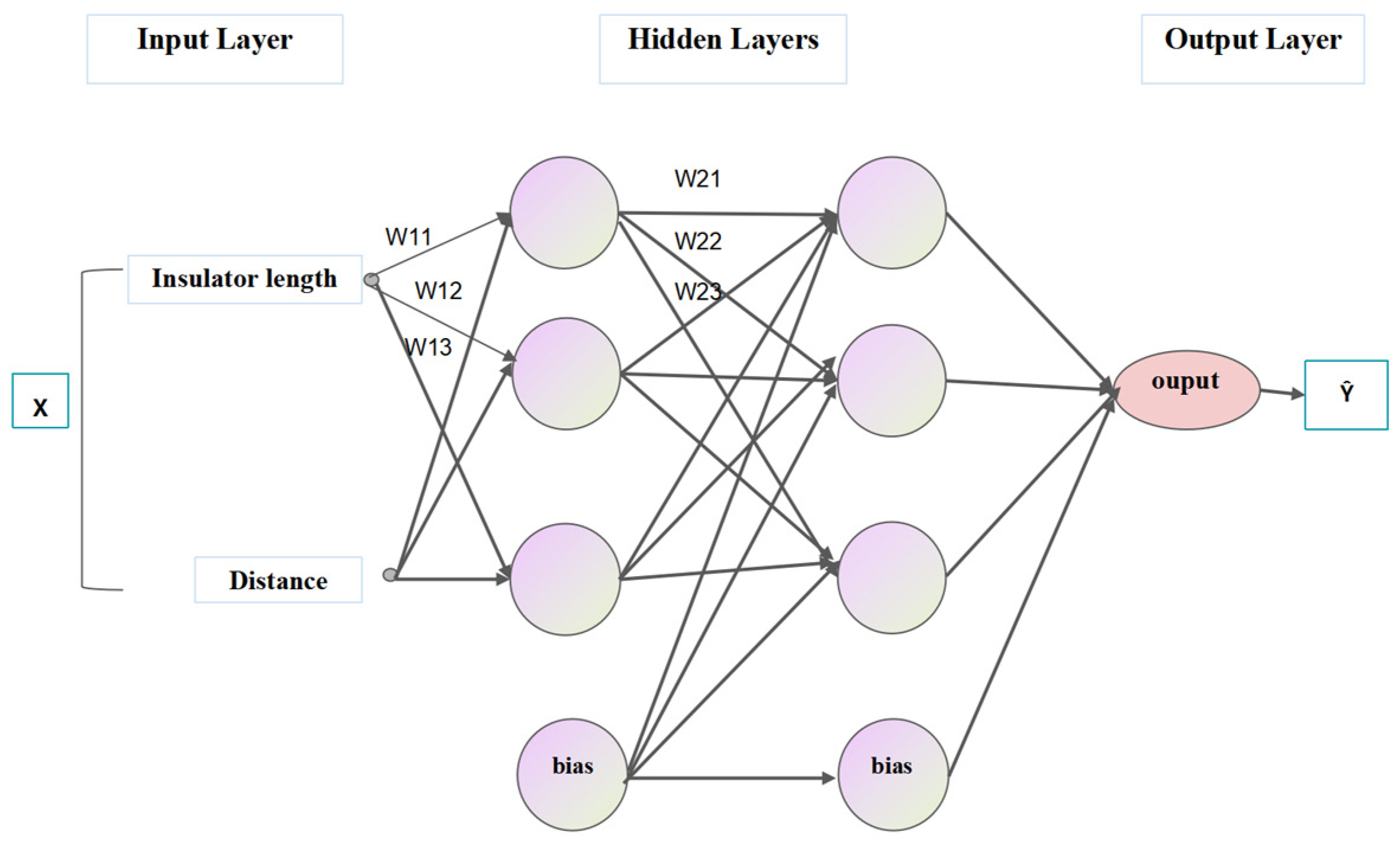
A three-layer MLP neural network model was employed to predict electric field intensity values based on two input parameters: the length of the insulator string (Insulator Length) and the distance of the measuring device from the insulator surface (Distance). The structure of the three-layer MLP model is illustrated in Figure 9, consisting of three primary components: an input layer, hidden layers, and an output layer. The input layer comprises two nodes corresponding to the two input variables: Insulator Length and Distance. The network features two hidden layers, each containing three neurons (also referred to as nodes). These neurons are interconnected with the input and subsequent layers through a set of weights (W). The primary function of the hidden layers is to perform complex nonlinear transformations on the input data, extracting higher-level feature representations from the raw data. The output layer contains a single node that represents and outputs the predicted electric field intensity value (Output) as the final result of the neural network’s computation. This architecture highlights the neural network’s robust capability to handle complex prediction tasks effectively.

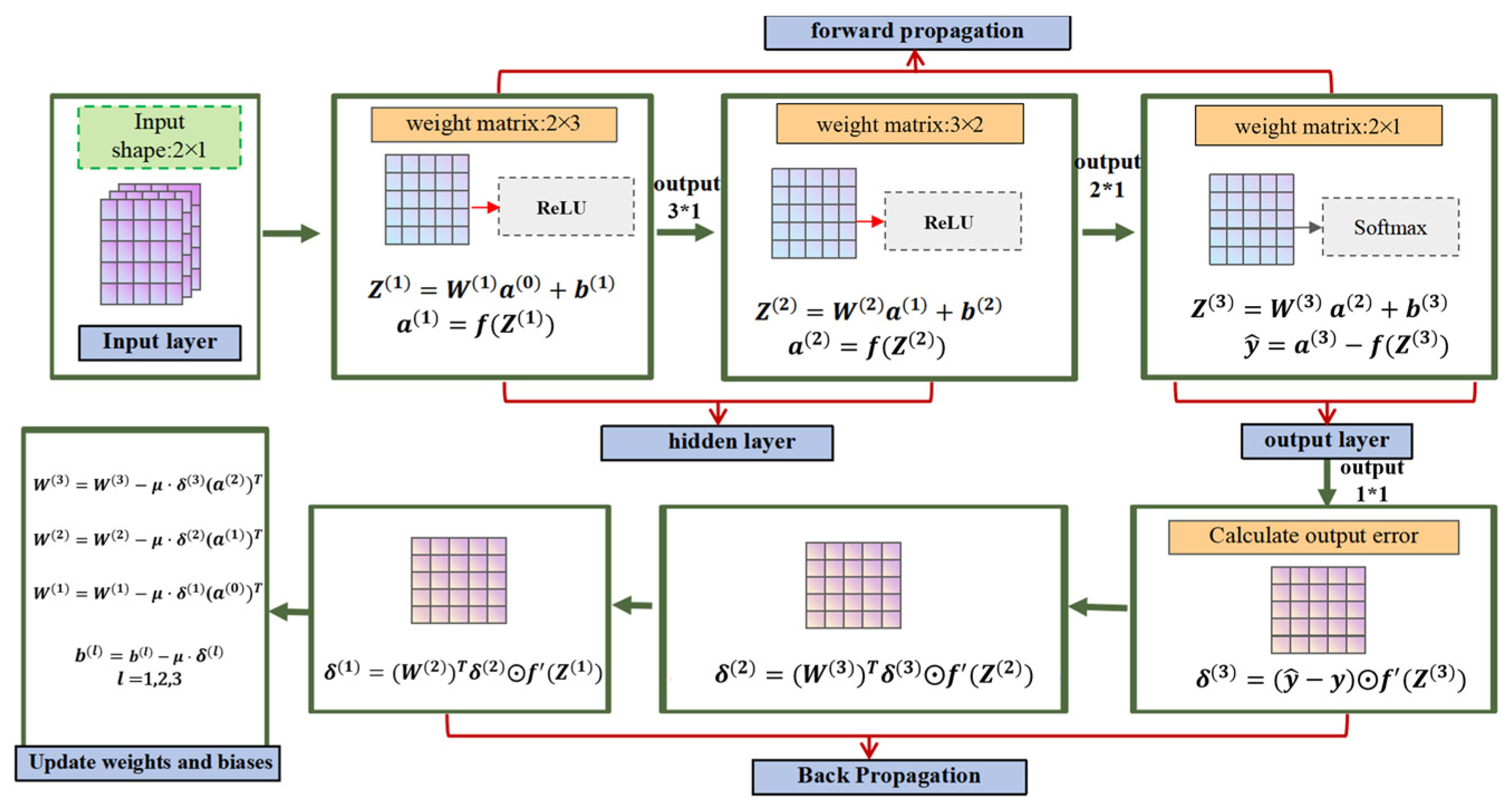
Figure 10 illustrates the working principles of the Multi-Layer Perceptron (MLP) neural network, which can be systematically divided into four core stages: forward propagation, loss computation, backpropagation, and iterative training. During the forward propagation stage, input data are fed into the input layer and subsequently passed to the first hidden layer through predefined weights (W). Each node in a hidden layer receives weighted inputs from all nodes in the preceding layer and applies an activation function (such as sigmoid or ReLU) to determine whether the node is “activated.” This activation mechanism propagates layer by layer until the output layer is reached, where the predicted electric field intensity value is generated. Next, the loss computation stage compares the predicted value with the actual electric field intensity using a specific loss function, such as mean squared error (MSE), to quantify the model’s prediction accuracy. A smaller loss value indicates higher prediction precision.

In the backpropagation stage, the gradient of the loss function is calculated, and optimization algorithms, such as gradient descent, are employed to iteratively adjust the network’s weights (W) and biases (Bias). These adjustments aim to minimize the loss function value and improve the model’s predictive performance. Finally, the aforementioned steps are repeated iteratively until the model converges, i.e., when the loss value decreases to a relatively small level. This process demonstrates the MLP neural network’s capability to optimize predictive accuracy through iterative training.

The mathematical symbols in the figure are defined as follows:

• Z: Weighted input vector.
• W: Weight matrix connecting adjacent layers.
• a: Activation output, where ReLU activation is applied to hidden layers and Softmax activation to the output layer.
• b: Bias vector.
• δ: Error term computed during backpropagation.
• ⊙: Hadamard product operator.

4.2. Analysis of Prediction Results

To evaluate the performance of the neural network model, commonly used regression metrics include:

Mean Squared Error (MSE): This metric quantifies the difference between the predicted and actual values. A smaller MSE indicates better predictive accuracy of the model.

$$\mathrm{M}\mathrm{S}\mathrm{E}={\displaystyle \frac{1}{\mathrm{K}}}\sum _{\mathrm{i}=1}^{\mathrm{K}}{\left(\mathrm{T}\mathrm{i}-\mathrm{Y}\mathrm{i}\right)}^2$$

(5)

where Ti represents the target value of the i-th sample, Yi is the predicted value, and K is the number of samples.

Coefficient of Determination (R²): This metric reflects the model’s explanatory power over the data. An R² value closer to 1 indicates a better model fit.

$$R^2={\displaystyle \frac{{\displaystyle {\sum }_{i=1}^K{\left(Yi-\stackrel{-}{T}\right)}^2}}{{\displaystyle {\sum }_{i=1}^K{\left(Ti-\stackrel{-}{T}\right)}^2}}}=1-{\displaystyle \frac{{\displaystyle {\sum }_{i=1}^K{\left(Ti-Y\mathrm{i}\right)}^2}}{{\displaystyle {\sum }_{i=1}^K{\left(Ti-\stackrel{-}{T}\right)}^2}}}$$

(6)

The model’s predictions are evaluated using two metrics: MSE = 3.89457 and R² = 0.88. For the evaluation of prediction performance: an R² value greater than 0.8 indicates a good predictive capability of the model.

The predictive performance of the model can also be evaluated by generating relationship curves between insulator string length and electric field intensity. Taking a detection distance of 200 mm as an example, the comparison between the model’s predicted values and simulation results is presented. Figure 11 illustrates the electric field intensity distribution of the seventh zero-value insulator, comparing simulation outcomes with model predictions. The trends of the simulation and prediction are largely consistent, demonstrating the model’s reliability and validity, with errors not exceeding 10%.

4.3. Experimental Validation of Prediction Outcomes

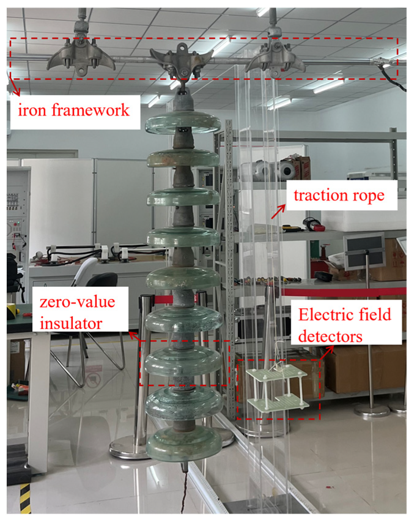
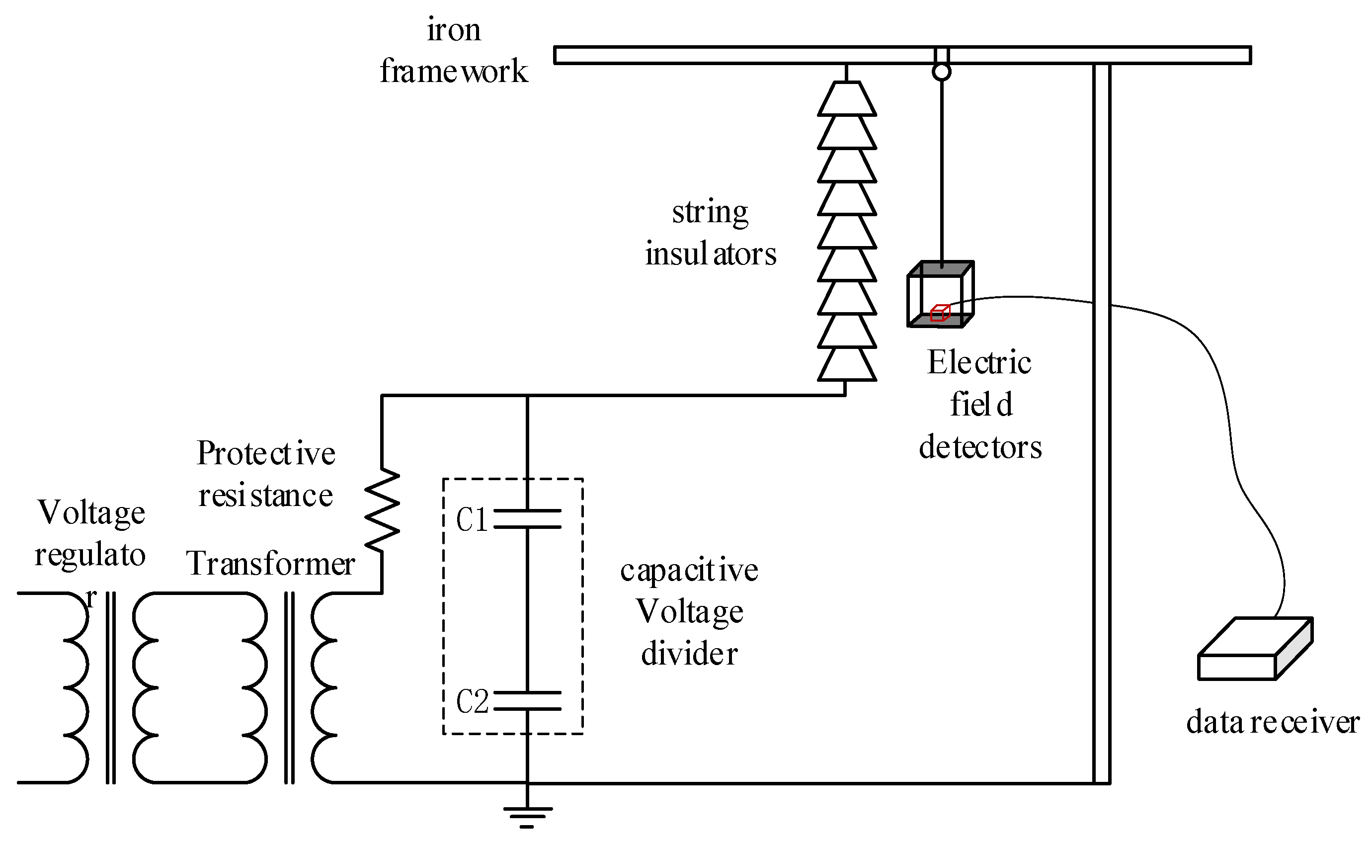
To verify the reliability of the proposed model, a degraded insulator detection test platform was constructed, as shown in Figure 12. A suspension string of nine XP-160 porcelain insulators was mounted on a cross-arm. The electric field detection device was placed inside a pod, which was secured using a pulley and a traction rope. The distance between the traction rope and the edge of the insulator string was maintained at approximately 200 mm. The detection device was uniformly pulled upward from the high-voltage end to the low-voltage end, measuring each insulator sequentially while recording the results. Degraded insulators were simulated by short-circuiting the steel caps and feet of porcelain insulators using conducting wires, with a degraded insulator placed as the third unit from the high-voltage end. The schematic diagram of the test wiring is provided in Figure 13. The voltage was supplied by the test power source, passed through a protective resistor, and applied to the high-voltage end of the insulator string via a capacitive voltage divider. The iron frame of the capacitive voltage divider and the low-voltage end of the insulator string were reliably grounded. Communication between the electric field detection device and the data-receiving terminal was established to ensure seamless data acquisition.

Due to the limitations of laboratory equipment, a voltage of 90 kV was applied in this experiment to simulate and evaluate the performance of degraded insulators on a 110 kV transmission line. The primary objective of the experiment was to validate the accuracy and effectiveness of the proposed model’s predictions through empirical testing.

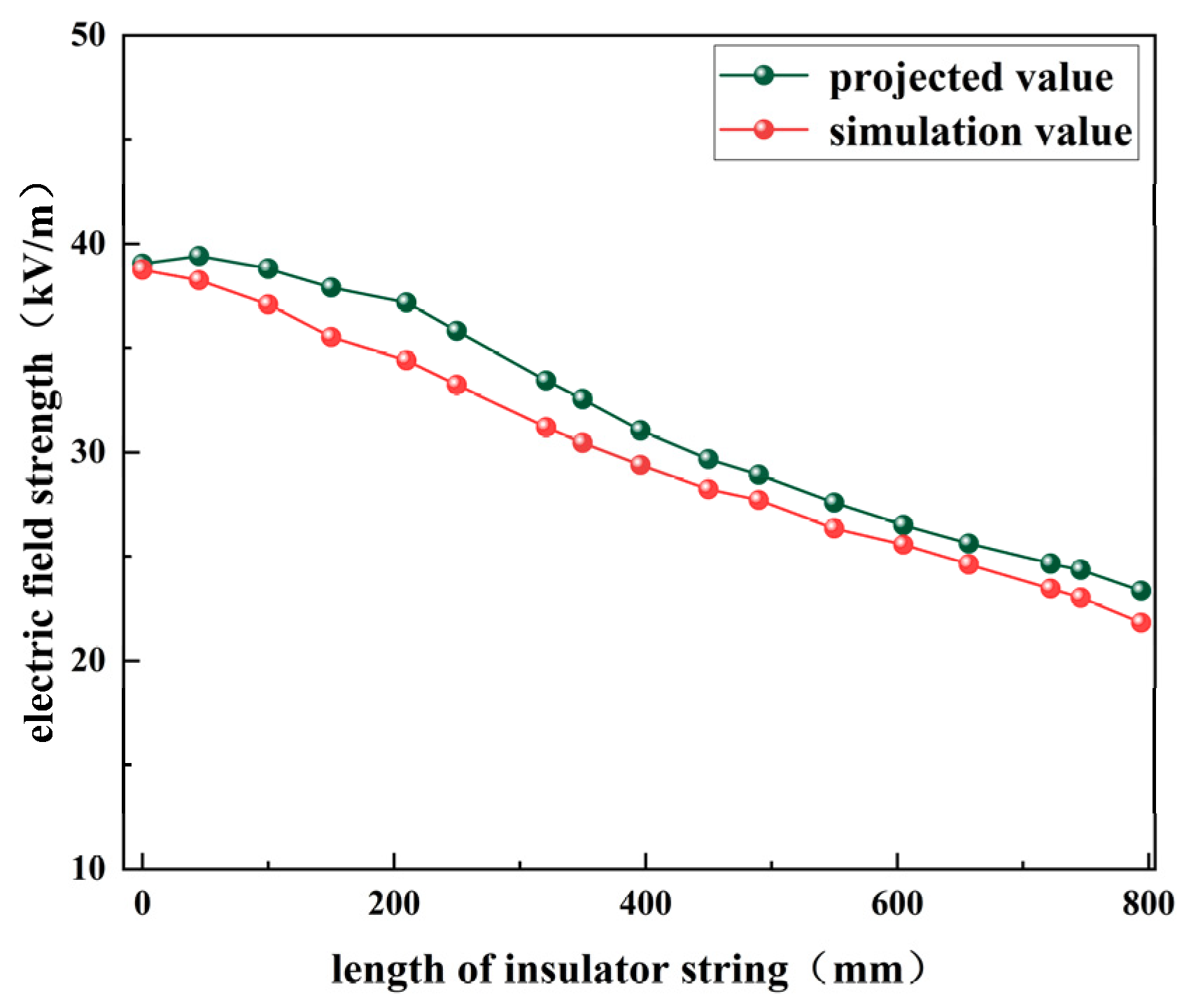
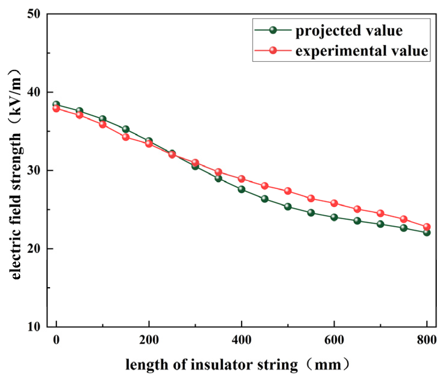
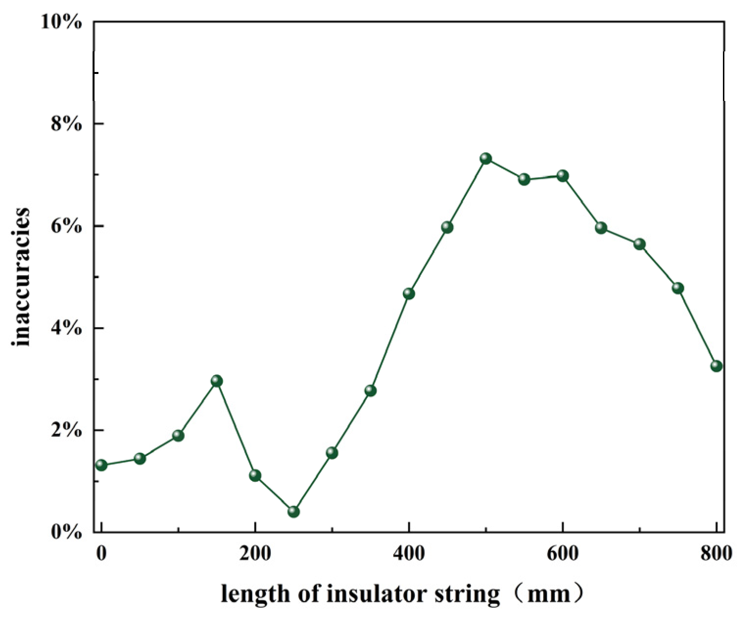
As shown in the data from Figure 14, the predicted electric field intensity at the first sampling point was 38.406 kV/m, while the corresponding experimental value was 37.9 kV/m, resulting in a calculated error rate of 1.31%. The maximum error occurred at the position where the insulator string length was 500 mm, with the predicted value being 25.356 kV/m compared to the experimental value of 27.357 kV/m, yielding an error rate of 7.32%. In contrast, the minimum error was observed near the second insulator, with an error rate of only 0.4%, Comparison between experimental and predicted values, as shown in Figure 15.

A comparison of the model’s predictions with experimental results reveals a high degree of consistency in overall trends, with all errors remaining within 10%. This finding partially validates the reliability of the model. However, it is noteworthy that significant deviations in electric field intensity were observed at different distances, likely due to discrepancies in insulator dimensions and experimental environmental conditions.

Further analysis reveals unavoidable differences between the experimental environment and the tower line and hardware structure set in the simulation model. As a result, there is a noticeable amplitude deviation between the actual measured and predicted electric field intensities at the same detection distance. These deviations highlight the need to thoroughly account for environmental factors affecting electric field distribution before applying the model to real-world engineering scenarios, necessitating appropriate calibration and optimization of the model.

5. Conclusions

This study employs electrostatic field simulation based on COMSOL to investigate the effects of detection distance, position, and quantity of zero-value insulators on electric field distribution. The spatial electric field distribution patterns of insulators were examined under various conditions and distances, leading to the following conclusions:

(1)

A detection distance of 20 mm allows for a significant reflection of the electric field strength variations near the porcelain insulator string. However, when the detection distance exceeds 300 mm, the response to zero-value insulators is diminished. Therefore, in practical engineering applications, it is recommended that the detection distance be controlled within the range of 20 mm to 300 mm.

(2)

In the three-dimensional electric field zero-value condition, the impact of degraded insulators diminishes with increasing measurement distance. The effect is more pronounced at the high-voltage end and the tower connection end, with minimal influence at the center. Additionally, continuous degradation of two insulators has a greater impact on the spatial electric field variation rate than intermittent or single insulator degradation.

(3)

To construct a spatial electric field distribution database for insulator strings with zero-value defects, a Multi-Layer Perceptron (MLP) neural network model was employed in this study. Its predictive accuracy was thoroughly validated through rigorous experiments. This database provides robust data support for insulator degradation detection, thereby enhancing the precision and reliability of insulator condition monitoring and analysis.

References

- Miao, C.; Wang, W.; Wang, R.; Chen, G.; Li, J.; Tang, W. Finite Element Analysis of Fracture and Size Optimization of Steel Pin Ball of Cap and Pin Type Suspension Insulator. Insul. Surge Arresters 2022, 1, 165–170. [Google Scholar]
- Ying, X.; Zhang, M.; Wang, S.; Qin, L. Design of a non⁃contact fault detection system for porcelain insulators based on laser excitation. Electron. Des. Eng. 2021, 29, 10–14. [Google Scholar]
- Li, J.; Lü, Y. Status Quo and Prospect of Research on Contamination Characteristics of Insulators. Guangdong Electr. Power 2018, 31, 18–23. [Google Scholar]
- Zeng, L.; Zhang, Y.; Zeng, X.; Li, T.; Deng, Z.; Wang, P.; Wan, H.; Xu, B.; Liu, Y.; Dong, C.; et al. Aging State Evaluation Methods for Silicone Rubber Sheds of Composite Insulators. Insul. Surge Arresters 2022, 2, 139–145+152. [Google Scholar]
- Li, Y.; Zhou, L.; Li, T.; Shao, X.; Chu, J.; Gao, L. Fault Analysis for Lightning Strike-caused String Fracture of 500 kV Line Porcelain Insulators. Zhejiang Electr. Power 2020, 39, 17–21. [Google Scholar]
- Jiang, Y.; Han, J.; Ding, J.; Fu, H.; Wang, Y.; Cao, W. The identification and Diagnosis of Self-Blast Defects of Glass Insulators Based on Multi-Feature Fusion. Electr. Power 2017, 50, 52–58+64. [Google Scholar]
- Zhang, Q.; Li, C.; Sun, Y.; Yang, C. Accurate Identification of Insulator Based on Deep Learning. Insul. Surge Arresters 2022, 1, 143–150. [Google Scholar]
- Zhou, Q. Sequence of Live Testing on Suspension Insulators Using Spark Gap Methodology. Electr. Saf. Technol. 2002, 3, 25–26. [Google Scholar]
- Chi, D.; Zeng, Q.; Sun, L. Detecting Insulator by UV Imaging. High Valtage Eng. 2006, 2, 115–116. [Google Scholar]
- Cheng, Y.; Xia, L.; Li, Z.; Cheng, D.; Yan, B.; Li, S. Detection of Zero-Value Ceramic Insulators Based on Infrared Imaging Methodology. Insul. Mater. 2019, 52, 74–79. [Google Scholar]
- Wang, S.; Jiang, T.; Li, W.; Lü, F.; Liu, P. Study on Infrared and UV Imaging Characteristics Test and Coupling Field Simulation of Zero-value Insulator Strings. High Volt. Appar. 2021, 57, 1–9. [Google Scholar]
- Ramesh, M.; Cui, L.; Gorur, R. Impact of superficial and internal defects on electric field of composite insulators. Int. J. Electr. Power Energy Syst. 2019, 106, 327–334. [Google Scholar] [CrossRef]
- Cheng, Y.; Li, C.; Ma, X. Study on Online Detection of Faulty Composite Insulators by Electric Field Method. High Volt. Eng. 2002, S1, 8–63. [Google Scholar]
- Xu, Y.; Lu, J.; Zhu, X.; Zhang, C.; Zhang, D.; Liu, X.; Huang, X. A Noncontaet Zero-value Insulator Detection Method and Device. Guangdong Electr. Power 2021, 34, 130–136. [Google Scholar]
- Zhang, D.; Chang, Z.; Wan, W.; Zhang, Z.; Chen, J. Zero-value insulator detection technology based on local electric field. Eletr. Power Eng. Tehnol. 2024, 43, 193–201. [Google Scholar]
- Liu, P.; Wu, Z.; Zhu, S.; Xu, J.; Liu, Q.; Peng, Z. Simulation on Eletric Field Distribution of 1 100kY AC Tri-Post Insulator Influenced by Defects. Trans. China Electrotech. Soc. 2022, 37, 469–478. [Google Scholar]