A Multi-Task Spatiotemporal Graph Neural Network for Transient Stability and State Prediction in Power Systems

Abstract

Transient stability assessments and state prediction are critical tasks for power system security. The increasing integration of renewable energy sources has introduced significant uncertainties into these tasks. While AI has shown great potential, most existing AI-based approaches focus on single tasks, such as either stability assessments or state prediction, limiting their practical applicability. In power system operations, these two tasks are inherently coupled, as system states directly influence stability conditions. To address these challenges, this paper presents a multi-task learning framework based on spatiotemporal graph convolutional networks that efficiently performs both tasks. The proposed framework employs a spatiotemporal graph convolutional encoder to capture system topology features and integrates a self-attention U-shaped residual decoder to enhance prediction accuracy. Additionally, a Multi-Exit Network branch with confidence-based exit points enables efficient and reliable transient stability assessments. Experimental results on IEEE standard test systems and real-world power grids demonstrate the framework’s superiority as compared to state-of-the-art AI models, achieving a 48.1% reduction in prediction error, a 6.3% improvement in the classification F1 score, and a 52.1% decrease in inference time, offering a robust solution for modern power system monitoring and safety assessments.

1. Introduction

Transient stability assessments and state prediction are essential functions of the EMS (Energy Management System) in power grid dispatch control centers. However, the global transition in energy structures and the growing focus on sustainable development have significantly increased the integration of renewable energy sources into power systems. The inherent intermittency and volatility of these sources present substantial challenges to grid stability [1]. Meanwhile, the advancement of smart grids has enabled bidirectional interaction and intelligent regulation, further increasing system complexity and uncertainty [2].

In this context, traditional methods for transient stability assessments and state prediction are increasingly inadequate for meeting the demands of modern power grids. Conventional approaches, including time-domain simulations, direct methods, and frequency-domain methods, each have distinct advantages and limitations. Among these, time-domain simulation [3] remains the most fundamental and widely adopted technique. By numerically integrating the power system’s dynamic equations, it provides a detailed time-domain response to disturbances, effectively capturing complex dynamic behaviors and nonlinear phenomena. However, its applicability to large-scale systems is often constrained by substantial computational demands and prolonged processing times.

Direct methods assess system stability by analyzing static and dynamic characteristics without relying on detailed time-domain simulations. Representative techniques include energy-based methods such as the Equal Area Criterion [4], the Energy Boundary Theorem [5], and the Lyapunov Method [6]. The Equal Area Criterion is computationally efficient, making it suitable for rapid stability assessments, while the Lyapunov Method offers strong theoretical guarantees for global stability analysis. However, constructing appropriate energy functions remains a significant challenge.

Frequency-domain methods [7], such as modal and oscillation analysis, evaluate transient stability based on the system’s frequency response. Modal analysis is particularly effective for detecting oscillatory behavior in large-scale systems and is well suited for small-disturbance scenarios. Oscillation analysis, meanwhile, provides deeper insights into dynamic system behavior but heavily depends on accurate models and parameters.

In recent years, the rapid advancement of artificial intelligence has created new opportunities for addressing the challenges of transient stability assessments and state prediction in power systems. Various AI approaches have demonstrated remarkable potential in power system applications. The Group Method of Data Handling (GMDH) neural networks have shown excellent performance in power system fault detection and load forecasting, with studies achieving fast fault detection times of around 20 ms [8] and mean absolute percentage errors as low as 2.10% [9] in demand forecasting. Additionally, deep learning and GNNs (Graph Neural Networks) have exhibited significant capabilities in handling complex temporal and graph-structured data.

For transient stability assessments, Reference [6] proposed an evaluation model leveraging CNNs (Convolutional Neural Networks) and hierarchical strategies, effectively enabling the real-time detection of impending instability and its patterns. To accommodate the evolving topologies of modern power systems, Reference [7] introduced a data-driven transient stability assessment framework based on deep forests. By incorporating an update scheme with active learning strategies, this approach enhanced model adaptability and robustness.

Inspired by the physical principles of power systems, Reference [10] developed a graph shift operator derived from power flow equations, facilitating the integration of spatiotemporal graph convolution with RNNs. While this approach showed favorable results in transient stability assessments, it lacks the ability to process multiple related tasks simultaneously, potentially missing important correlations between system states and stability conditions. Similarly, Reference [11] combined GCN with LSTM units to form a recurrent graph convolutional network. Although this architecture effectively incorporates bus states and topological features through GCNs and captures temporal dependencies via LSTM units, its fixed-depth network structure may lead to unnecessary computational overhead for simple samples while being insufficient for complex cases.

For power system state prediction, Reference [12] proposed an artificial-neural-network-based model that employs a two-step filtering and prediction process. While this approach surpasses traditional methods in speed and accuracy, its simplified network structure limits its ability to capture complex spatial correlations in large-scale power systems. To capture long-term nonlinear dependencies in voltage time series, Reference [13] applied deep RNN for state prediction. However, this method focuses solely on temporal patterns while overlooking the important spatial relationships between different buses. Additionally, to mitigate uncertainties associated with renewable energy integration, Reference [14] developed a physics-informed DNN for real-time power system monitoring. Although this model outperforms conventional solvers in terms of robustness, its single-task nature requires separate models for stability assessments and state prediction, increasing overall system complexity and computational costs.

Despite extensive research on AI-based transient stability assessments and state prediction in power systems [15,16,17,18,19,20], most existing models are designed for single-task applications. Consequently, they lack the ability to simultaneously perform both transient stability assessments and state prediction, limiting their practicality in addressing the complex demands of real-world power system operations.

To address these challenges, this paper proposes a novel multi-task learning framework based on GCNs that simultaneously performs transient stability assessments and state prediction in power systems. The framework leverages STGCNs (Spatiotemporal Graph Convolutional Networks) as the primary encoder, effectively capturing and utilizing both the topological and temporal characteristics inherent in power systems. It comprises two specialized branches: a self-attention U-shaped residual decoder, which predicts key graph-based variables such as bus voltage magnitudes and phase angles for precise state prediction, and a Multi-Exit Network branch, which incorporates multiple exit points at varying depths to provide reliable transient stability assessments based on predefined confidence thresholds. The multi-exit mechanism dynamically optimizes computational pathways while maintaining high accuracy, thereby significantly enhancing computational efficiency. By leveraging the synergistic interaction between these branches, the proposed framework enables an efficient and accurate evaluation and prediction of critical power system states. The main contributions of this paper are as follows:

• Innovative multi-task GCN framework:
  this paper introduces a novel GCN-based framework that seamlessly integrates transient stability assessments and state prediction, providing a unified solution for power system state analysis.
• Advanced Decoder Architecture: the self-attention U-shaped residual decoder effectively predicts key graph-based variables, including the bus voltage magnitude, phase angle, active power, and reactive power, ensuring precise state prediction.
• Efficient Multi-Exit Network Design: a Multi-Exit Network branch is proposed to dynamically optimize computational pathways based on confidence thresholds, significantly improving computational efficiency while maintaining accurate and reliable transient stability assessments.

Extensive experiments conducted on IEEE standard test systems and real-world power grids validate the superior performance of the proposed method. The results demonstrate that the multi-task GCN framework significantly surpasses existing approaches in both transient stability assessments and state prediction tasks, providing a robust and efficient solution to modern power system challenges. Compared to traditional methods, the proposed framework achieves a 6.3% improvement in the F1 score, reduces the prediction error by 48.1%, and decreases the inference time by 52.1%, demonstrating its effectiveness in handling the increasing complexity of modern power systems while maintaining high accuracy and computational efficiency.

2. Related Work

2.1. Graph Neural Networks

In recent years, GNNs have made significant advancements in processing graph-structured data and have been extensively applied in power system analysis. In the field of state prediction, Reference [21] addresses the limitations of traditional methods in capturing the dynamic characteristics of power systems. By integrating Kalman filter-based state prediction into the training process of GCNs, this approach enhances the reliability of GCNs for power system applications. However, the large-scale integration of renewable energy sources introduces substantial intermittency and uncertainty, further increasing the volatility and unpredictability of power systems. To mitigate these challenges, Reference [22] incorporates self-attention mechanisms into GCNs within the context of heterogeneous renewable energy sources and proposes an adaptive graph framework to exploit hidden spatiotemporal dependencies across multiple time scales for power system state prediction.

In the field of transient stability assessments, end-to-end models based on GCNs offer significantly faster computation compared to traditional numerical simulation methods. Reference [23] employs an enhanced GCN framework that aggregates global, node, and edge features of power systems, achieving transient stability assessments through a final fully connected layer. Building upon this, Reference [24] incorporates temporal features into GCNs and proposes a Temporal–Spatial Graph Convolutional Network algorithm. To further accelerate computation, a graph simplification strategy is introduced, compressing feature matrices related to grid topology and node information.

Despite the significant advancements of GCNs in transient stability assessments and state prediction, no research has yet comprehensively integrated these two applications into a unified framework.

2.2. Multi-Task Learning

Multi-task learning (MTL) offers an effective approach for simultaneously performing transient stability assessments and state prediction by sharing a unified feature extraction network and jointly learning multiple related tasks [25]. In power system research, MTL has been successfully applied across various domains. For instance, in load forecasting, Reference [26] proposed a deep learning framework that integrates MTL with CNN and LSTM networks to predict both short-term and medium-term electrical loads. Similarly, Reference [27] introduced a multi-energy short-term load forecasting method based on MTL, employing load participation factors to represent the contributions of different loads to total demand and exploring their coupling relationships to enhance forecasting accuracy.

In fault diagnosis, Reference [28] utilized a shared backbone GNN to jointly perform classification and detection of distribution system faults. Reference [29] developed an MTL framework that leverages CNNs and graph attention networks for the real-time assessment of transient angle stability and transient voltage stability. Notably, Reference [11] proposed an online transient stability assessment framework that integrates GCNs and LSTM into a recurrent graph Convolutional Neural Network. In this framework, the GCN captures bus states and topological features while the LSTM models temporal dynamics, enabling simultaneous stability classification and critical generator identification.

2.3. Multi-Exit Network

Multi-Exit Networks are specialized architectures designed to improve the inference efficiency of deep neural networks by introducing multiple output branches at different depths within the network. This design enables the model to dynamically determine whether to terminate computation early based on the complexity of the input sample and the confidence of the prediction, thereby reducing computational overhead [11]. The adaptive early exit mechanism offers substantial benefits in scenarios requiring high real-time performance.

In the field of deep learning, Multi-Exit Networks have been widely applied to tasks such as image classification and natural language processing. For instance, BranchyNet introduces multiple exits within deep networks, significantly accelerating inference while maintaining high accuracy. Similarly, Reference [14] proposed a multi-scale, multi-exit architecture that further optimizes inference efficiency. These studies demonstrate that Multi-Exit Networks can effectively reduce computational costs without compromising model performance, thereby enhancing both the flexibility and adaptability of models in practical applications. However, while Multi-Exit Networks have achieved significant success in various deep learning tasks, their potential in transient stability assessments and state prediction for power systems represents a promising direction for further investigation.

3. Power System Model

3.1. Graph Model

In this paper, the input data for all models are constructed based on the physical topology and operating characteristics of the power system. Specifically, the buses in the power system are treated as nodes, while the transmission lines connecting these buses are represented as edges, as shown in Figure 1.

Based on graph theory, this paper represents the state of the power system using feature matrices and adjacency matrices. Let the set of nodes in the graph be denoted as $\mathcal{N}$ and the set of edges as $\epsilon$. Each node in $\mathcal{N}$ corresponds to a bus in the power system, while each edge in $\epsilon$ represents a physical transmission line connection between buses. The entire power system can be modeled as graph data $\mathcal{G}=(\mathcal{N},\epsilon )$.

To perform transient analysis, several electrical factors need to be determined, including the voltage magnitude, phase angle, active power and reactive power at each bus. These electrical measurements form the feature vector for each node, capturing the dynamic operating state of the corresponding bus. The system’s operation duration is set to T, and the sampling interval is $\tau$, allowing it to be divided into several time slots $T=\left\{\tau ,2\tau ,\cdots ,\left|T\right|\right\}$. Therefore, the electrical factors of the power system can be represented in the form of a state matrix $X\in {\mathbb{R}}^{\left|\mathcal{N}\right|\times \left|T\right|\times 4}$, as follows:

$$G=\left[\begin{array}{cccc}{x}_{11}& x_{12}& \cdots & x_{1\left|T\right|}\\ x_{21}& x_{22}& \cdots & x_{2\left|T\right|}\\ ⋮& ⋮& \ddots & ⋮\\ x_{\left|\mathcal{N}\right|1}& x_{\left|\mathcal{N}\right|2}& \cdots & x_{\left|\mathcal{N}\right|\left|T\right|}\end{array}\right]$$

(1)

where $x_{i,t}^T=\left[\left|V_{i,t}\right|,{\theta }_{i,t},P_{i,t},Q_{i,t}\right],\forall i\in \mathcal{N},t\in T$, $\left|\mathcal{N}\right|$ denotes the number of nodes, ${\left(•\right)}^T$ denotes the transpose of a matrix, $\left|V_{i,t}\right|$ denotes the voltage magnitude, ${\theta }_{i,t}$ represents the voltage phase angle, $P_{i,t}$ signifies the active power, and $Q_{i,t}$ represents the reactive power.

The connection relationships between buses can be represented using an adjacency matrix $A\in R^{\left|\mathcal{N}\right|\times \left|\mathcal{N}\right|}$. The elements of matrix A are defined as follows:

$$A=\left\{\begin{array}{cc}1,\hfill & \mathrm{if}\mathrm{node}i\mathrm{is}\mathrm{connected}\mathrm{to}\mathrm{node}j\hfill \\ 0,\hfill & \mathrm{if}\mathrm{node}i\mathrm{is}\mathrm{not}\mathrm{connected}\mathrm{to}\mathrm{node}j\hfill \end{array}\right.$$

(2)

It is common practice to add self-loops to the adjacency matrix, i.e., introducing a self-connecting edge for each node to obtain a new adjacency matrix $\tilde{A}=A+I$, where I is the identity matrix. To balance the contribution of each node when aggregating information from its neighbors and to prevent high-degree nodes from exerting excessive influence, the adjacency matrix is typically subjected to degree normalization. The degree-normalized adjacency matrix is defined as $\widehat{A}={\tilde{D}}^{-{\displaystyle \frac{1}{2}}}\tilde{A}{\tilde{D}}^{-{\displaystyle \frac{1}{2}}}$, where $\tilde{D}$ is the degree matrix representing the total number of connections for each node, including self-loops.

3.2. Problem Definition

Considering both the spatial structure and the temporal dependencies of the power system, we define the state prediction task as a temporal graph prediction problem. As described in Section 3.1, by modeling the power system network as a directed graph $\mathcal{G}=(\mathcal{N},\epsilon )$, the problem can be formulated as follows:

$$\left[X_{t-T+1},\cdots ,X_t;\mathcal{G}\right]\stackrel{f_D\left(f_B(·)\right)}{\to }\left[X_{t+1},\cdots ,X_{t+H}\right]$$

(3)

Herein, T represents the length of time steps selected for the input data and H represents the length of the predicted time step while $f_D(·)$ represents the decoder network and $f_B(·)$ represents the backbone network. The transient stability assessment task is defined as a multi-exit binary classification problem, where each exit processes features at different depths and produces binary classification results. In our study, four outputs were configured, and their associated formulations are expressed as follows:

$$\left[X_{t-T+1},\cdots ,X_t;\mathcal{G}\right]\stackrel{f_C^1\left(f_B(·)\right),\cdots ,f_C^4\left(f_B(·)\right)}{\to }\left[Y_1,Y_2,Y_3,Y_4\right]$$

(4)

Here, $f_C^i(·)$ represents the classification network for the i-th output.

4. Temporal Graph Multi-Task Net

In this section, we first present an overview of the proposed model, termed the Temporal Graph Multi-Task Network (TGMT-Net). The primary objective of TGMT-Net is to leverage advanced GCN technologies to perform multi-task learning on temporal graph data. Specifically, one task focuses on predicting the state graph data of the power grid while the other involves classifying graph data using a multi-exit mechanism. We then discuss the design principles and functionalities of each module within TGMT-Net, followed by a detailed explanation of the model’s training loss.

4.1. TGMT-Net

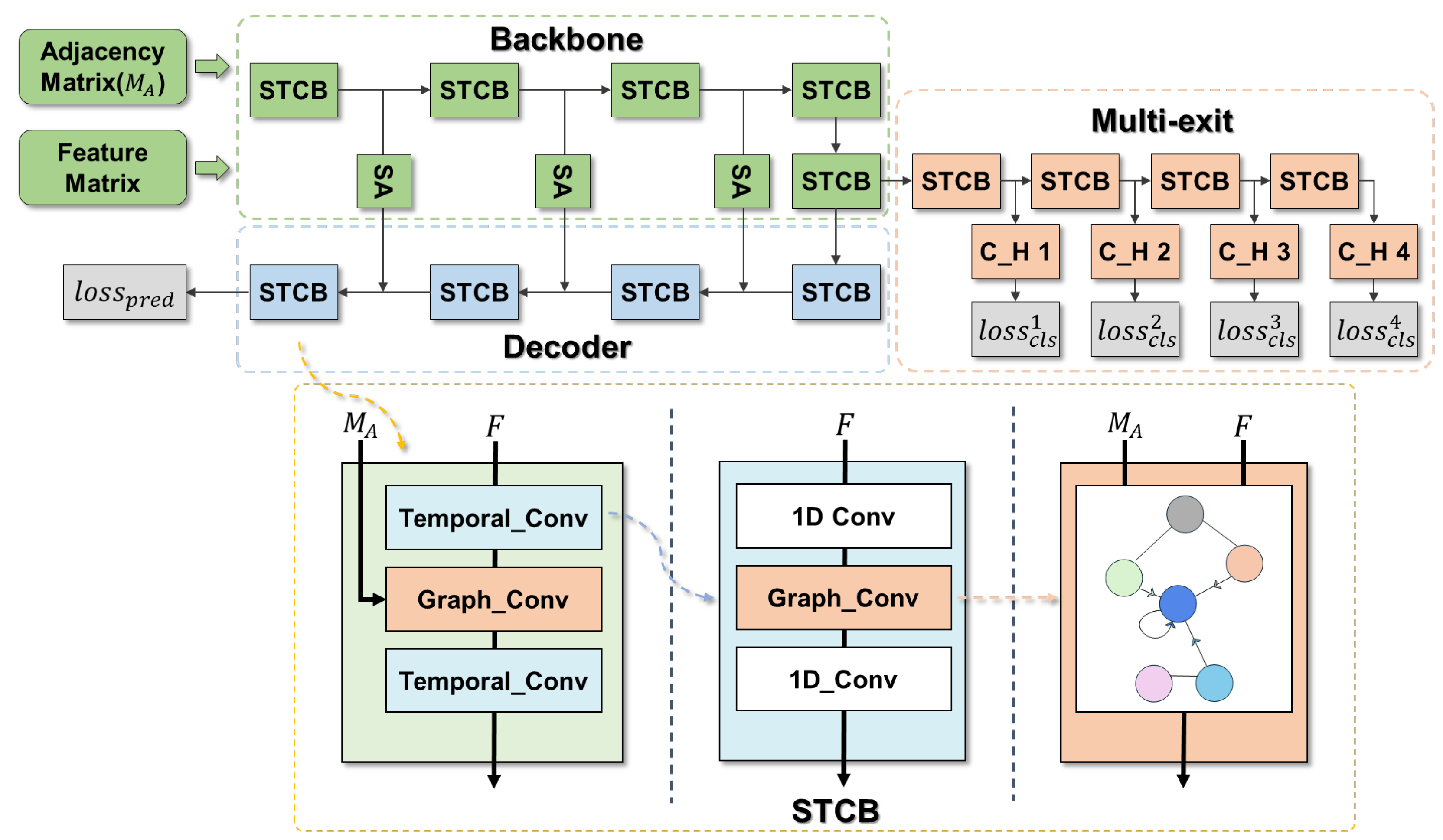
This study presents an advanced model, TGMT-Net, designed to perform state prediction and transient stability assessments in power systems using temporal graph data. The model effectively captures the inherent spatiotemporal dynamics of these graphs by simultaneously addressing both state prediction and classification tasks via a shared backbone network. For the prediction task, TGMT-Net uses a U-shaped self-attention network architecture to predict the states of the power system. For the classification task, it utilizes a multi-exit mechanism to achieve the efficient and reliable classification of graph data. The overall structure of TGMT-Net is illustrated in Figure 2.

Within the shared backbone network, the model first applies spatiotemporal graph convolution operations to extract temporal and spatial features from the input graph data. The classification module similarly employs spatiotemporal graph convolutions for feature extraction, but it incorporates a multi-exit mechanism. This mechanism enables the model to produce classification results from multiple intermediate layers and to terminate computations early when the classification confidence exceeds a specified threshold, thereby improving inference efficiency. Meanwhile, the prediction module adopts a self-attention Unet architecture that leverages the hierarchical features extracted from the shared backbone network to reconstruct future graph states.

Through this design, the model efficiently integrates multiple tasks. Both the state prediction and graph data classification tasks share spatiotemporal feature representations, ensuring high prediction accuracy while enhancing classification efficiency. This multi-task learning approach enables the model to perform complex power grid data analysis without incurring additional computational costs.

4.2. Self-Attention U-Shaped Residual State Prediction Module

To enhance the precision of state prediction, we designed a prediction module built upon spatiotemporal graph convolution layers that is seamlessly integrated with a shared backbone network. This integration yields a classic Unet. Within this framework, the encoder employs a series of spatiotemporal graph convolution layers to iteratively extract intricate spatiotemporal features from power grid data. These layers effectively capture both the spatial correlations among nodes in the power grid and the temporal dynamics underlying their interactions. In the decoder, the multi-level features distilled by the encoder are leveraged through spatiotemporal graph convolutions and adaptive pooling mechanisms, enabling the generation of accurate and reliable state predictions. The decoder architecture is illustrated in Figure 2.

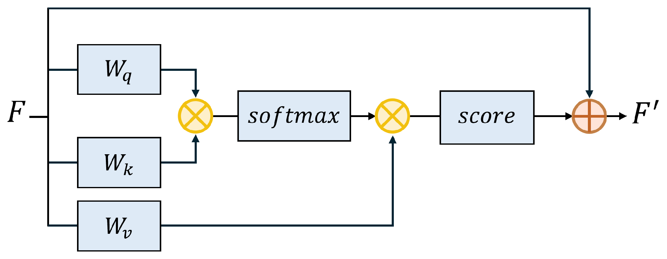
To connect the encoder and decoder, we incorporate self-attention modules as skip connections. These self-attention-based skip connections establish direct correspondences between encoder and decoder layers, enhancing the efficient transmission of multi-scale information across diverse feature hierarchies. By leveraging the self-attention mechanism, the model computes correlations among different positions within the feature maps, enabling it to adaptively prioritize critical nodes and time segments essential for state prediction. This dynamic reallocation of attention empowers the model to concentrate on key spatiotemporal regions, thereby improving its ability to extract and represent salient features with precision. The structure and functionality of these self-attention modules are illustrated in Figure 3.

These self-attention skip connections not only enhance the efficiency of feature transmission but also significantly improve the model’s robustness and generalization capabilities. By creating associations across multiple feature scales, the model achieves a deeper comprehension of the hierarchical structure in power grid data. This mechanism mitigates the risk of information loss during feature propagation, ensuring the retention of critical details. Consequently, the proposed design enables the model to achieve accurate state prediction while effectively handling complex and dynamic power system data.

4.3. Transient Stability Assessment Module

Building upon the shared backbone network, we developed a multi-exit early exit graph classification module specifically designed for transient stability assessments in power systems. This module introduces multiple exit nodes at various depths within the network, enabling dynamic decision making during inference. Specifically, the model evaluates prediction confidence at each exit point, and if the confidence surpasses a predefined threshold, the inference process halts and the current prediction is output.

This design achieves an optimal balance between inference speed and accuracy. For instances characterized by simplicity or distinct features, high-confidence predictions can be generated at shallower layers, bypassing the need for computationally expensive deeper layers. This significantly reduces computational overhead and satisfies the real-time monitoring demands of power systems. Conversely, for complex or ambiguous cases, the model proceeds to deeper layers until the required confidence level is reached, ensuring the reliability of assessment outcomes, as illustrated in the multi-exit block of Figure 2.

The effectiveness of the multi-exit early exit mechanism depends on the careful calibration of confidence thresholds at each exit. These thresholds are fine-tuned using performance metrics on the validation set to optimize the model’s overall performance. This adaptive mechanism allows the model to adjust its computational depth based on the complexity of input samples. For example, in transient stability assessments, fault modes with distinct features can be rapidly identified at earlier stages, while intricate fault scenarios necessitate deeper feature extraction and analysis to ensure accurate assessments.

4.4. Loss Function

In our model, distinct loss functions are meticulously designed for each task to facilitate effective learning and optimization. For the state prediction task, the Mean Squared Error (MSE) is employed as the loss function, owing to its suitability for regression problems. The MSE quantifies the average squared difference between the predicted and actual values, thereby driving the model to minimize prediction errors. The formulation of the MSE loss function is as follows:

$${loss}_{pred}={(y-\widehat{y})}^2$$

(5)

Here, $\widehat{y}$ denotes the predicted value and y denotes the label. For the transient stability assessment task, our objective is to determine whether the power system is currently in a stable state, which constitutes a binary classification problem. Due to the class imbalance in the dataset (with unstable states being the minority class), directly using standard Cross-Entropy Loss may result in the model being biased toward the majority class. To mitigate this, we adopt a weighted combination of Cross-Entropy Loss and Focal Loss, formulated as follows:

$${loss}_{cls}=\alpha \times \left(-\sum _{i=1}^2{y}_{i}log{\widehat{y}}_i\right)+\left(1-\alpha \right)\times [-\sum _{i=1}^2{(1-{\widehat{y}}_i)}^{\gamma }{y}_{i}log{\widehat{y}}_i]$$

(6)

Here, $\gamma$ is a hyperparameter that controls the emphasis placed on easy versus hard samples. By weighting and combining these two loss functions, our model achieves a balance between overall classification accuracy and the capacity to effectively identify minority class samples. The Cross-Entropy Loss ensures accurate classification for the majority of samples, while the Focal Loss directs the model’s attention to challenging, hard-to-classify, and imbalanced minority class instances. The hyperparameter $\alpha$ balances the relative contributions of the standard Cross-Entropy Loss and the Focal Loss component in the overall classification loss. This approach enhances the model’s ability to detect unstable states in the power grid, improving the performance of transient stability assessments. In our study, we choose $\gamma$ = 2 and $\alpha$ = 0.4. The total loss of the network is as follows:

$${loss}_{total}={loss}_{pred}+\sum _{i=1}^4{\beta }_i{loss}_{cls}^i$$

(7)

Here, ${loss}_{cls}^i$ denotes the classification loss at the i-th exit. In this paper, the corresponding weights ${\beta }_i$ for the four exits (from shallow to deep layers) were assigned values of 0.1, 0.2, 0.3, and 0.4, respectively.

5. Results

5.1. Evaluation Metrics

For model evaluation, we selected appropriate metrics for different tasks to assess the model’s performance and applicability. For the state prediction task, the following evaluation metrics were used:

$$MAE={\displaystyle \frac{1}{n}}\sum _1^n\left|y-\widehat{y}\right|$$

(8)

For the transient stability assessment task, which is a binary classification (stable or unstable) and may involve class imbalance, we employed the following evaluation metrics:

$$Accuracy={\displaystyle \frac{TP+TN}{TP+TN+FP+FN}}$$

(9)

$$Recall={\displaystyle \frac{TP}{TP+FN}}$$

(10)

$$Precision={\displaystyle \frac{TP}{TP+FP}}$$

(11)

$$F1Score=2\times {\displaystyle \frac{Precision\times Recall}{Precision+Recall}}$$

(12)

Here, $TP$ (True Positive) and $TN$ (True Negative) represent the number of samples correctly identified as stable and unstable, respectively. $FN$ (False Negative) denotes the number of samples incorrectly identified as stable, while $FP$ (False Positive) denotes the number of samples incorrectly identified as unstable.

5.2. Experimental Details

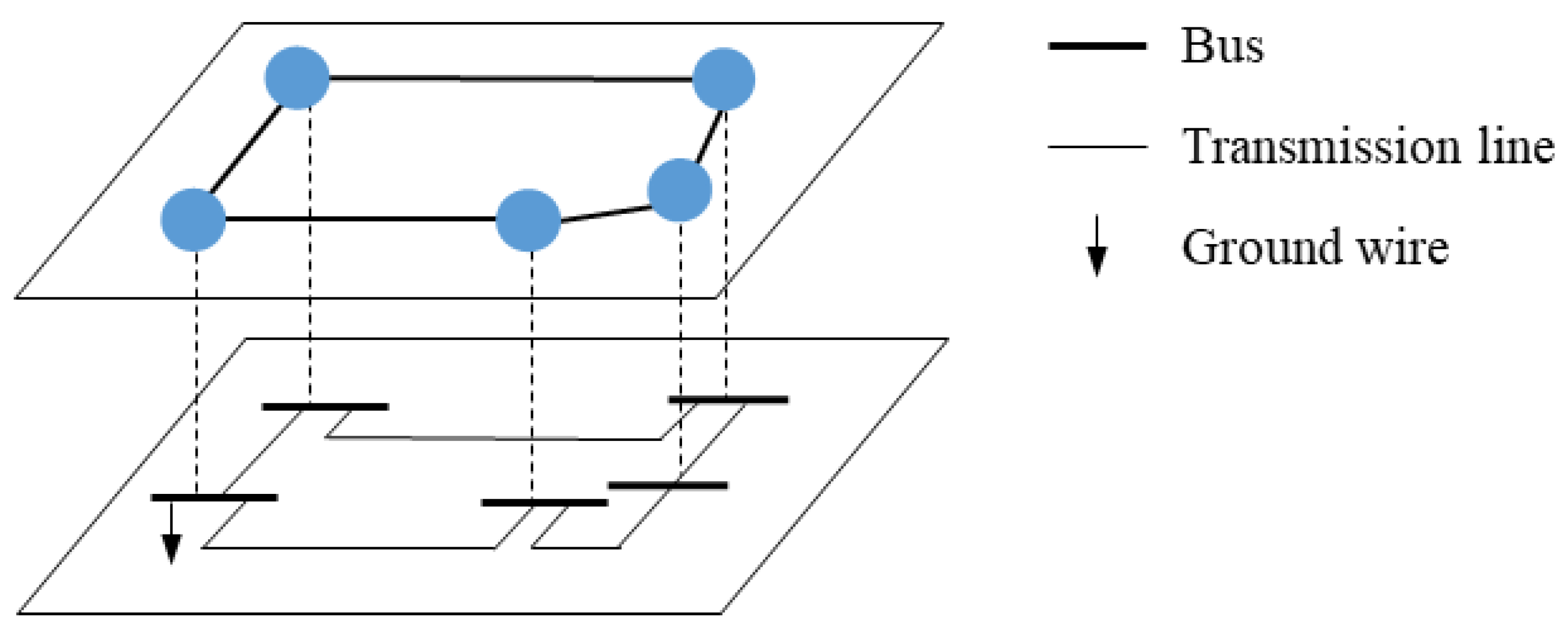
In the experiment, we used three power system standard examples of different scales for case studies: the IEEE 68-bus system, the IEEE 145-bus system, and a provincial power grid system. For each power system, we extracted data such as buses and lines in the IEEE general data format. The details of the three test cases are as follows:

• IEEE 68-bus system: the system consists of 68 buses and 89 transmission lines, simulating the topology of a medium-sized power network.
• IEEE 145-bus system: this system includes 145 buses and 153 transmission lines, simulating the structure of a high-voltage transmission network.
• A real provincial power grid system: composed of 139 buses, encompassing multiple power plants, substations, and numerous transmission lines, comprehensively simulating the complex topology of real-world power networks.

The datasets for these three systems are obtained through simulations in DSP Studio V2. They are generated by randomly introducing N-2 faults on the transmission lines, with the fault duration set to 120 ms. The system’s sampling interval is 10 ms, and the total sampling duration is 20 s. The sampled data include the bus voltage magnitude, bus voltage phase angle, bus active power, and bus reactive power. We select a continuous sequence of 48 time steps from the sampled data as one sample, with the first 32 time steps used as input (T = 32), the subsequent 16 time steps as labels for state prediction (H = 16), and the system’s instability status serving as the sample’s classification label.

All experiments were conducted using PyTorch (version 1.12.1) on a hardware platform consisting of an NVIDIA A6000 GPU and an Intel i9-12900K CPU. The dataset underwent stratified random sampling to maintain balanced distributions of stable and unstable cases across training (70%), validation (20%), and test (10%) sets. Prior to training, all input features were normalized to [0, 1] using min–max scaling.

The network was trained for 400 epochs with a batch size of 32, where the batch size was empirically determined to optimize the trade-off between computational efficiency and model convergence. We employed a cosine annealing learning rate schedule initialized at $2\times {10}^{-4}$ and gradually decaying to $1\times {10}^{-6}$. To prevent overfitting, we implemented early stopping with a patience of 20 epochs by monitoring the validation loss. The model weights corresponding to the minimum validation loss were preserved for subsequent evaluation on the test set.

For inference on the test set, we implemented an early exit mechanism with a confidence threshold of 0.95. Specifically, if any exit produces a class probability exceeding 0.95, the inference process terminates immediately. Otherwise, the forward propagation continues through all exits. In cases where no exit achieves the confidence threshold, the final classification is determined by taking the mode of the predictions from the last three exits.

5.3. Model Comparison

To validate the effectiveness of the proposed multi-task model on the transient temporal graph data of power systems, we conducted comparative experiments with traditional models for both graph data prediction and graph classification tasks.

In the task of graph data prediction, we selected several traditional graph sequence models for comparison. The GCN-GRU model combines GCNs with Gated Recurrent Units (GRUs) to process spatiotemporal graph data for prediction. In this model, a GCN is employed to learn the structural information of the graph by aggregating data through node adjacency relations, thereby capturing the spatial dependencies within the graph structure. GRUs, as the temporal modeling units, effectively capture long-term dependencies in time series data through their gating mechanism. The advantage of the GCN-GRU model lies in its ability to handle both spatiotemporal graph data, making it suitable for complex prediction tasks involving both temporal and structural dependencies.

The STGCN model captures spatiotemporal correlations for prediction by combining temporal convolution with graph convolution. It learns the spatial features of the graph through hierarchical graph convolution networks and captures temporal dependencies via temporal convolution modules. Its innovation lies in separately handling graph structural and temporal information, which enables a more efficient capture of spatiotemporal relationships in graph data.

The graph attention network (GAT) enhances the GCN by introducing an attention mechanism that assigns different weights to neighboring nodes, thereby improving the model’s expressive power. In GAT, a self-attention mechanism is applied in each graph convolution layer, allowing each node to dynamically adjust the weights based on its neighboring nodes’ features. This approach enables the model to more flexibly capture the importance of neighboring nodes, enhancing its ability to extract relevant information for graph-level tasks.

Our proposed model integrates a multi-output classification network following the GCN encoder, with four classifier outputs at different depths. These outputs are designed to exit adaptively based on confidence levels, thereby enhancing both classification efficiency and accuracy.

In terms of evaluation metrics, we used the MAE to evaluate the graph data prediction tasks. For the graph classification task, classification accuracy, precision, recall, F1 score, and inference time were employed to comprehensively assess the model’s performance.

Table 1. Compare the predictive performance of different methods.

Methods	IEEE 68 MAE	IEEE 145 MAE	My Data MAE
GCN-GRU	0.0129 ± 0.0033	0.0297 ± 0.0092	0.0337 ± 0.0104
GAT	0.0059 ± 0.0019	0.0177 ± 0.0046	0.0218 ± 0.0055
STGCN	0.0067 ± 0.0026	0.0206 ± 0.0062	0.0274 ± 0.0078
Ours	0.0046 ± 0.0014	0.0102 ± 0.0027	0.0127 ± 0.0033

presents the experimental results, indicating that in the prediction task, the proposed model significantly outperforms the comparison models on all datasets, demonstrating its superior performance. On the IEEE 68-bus dataset, the MAE of the proposed model is 0.0046 ± 0.0014, which represents a 22.0% reduction in error compared to the best-performing comparison model, GAT, and a significant 64.3% reduction compared to GCN-GRU. This improvement in the MAE translates into more accurate voltage stability margin predictions in actual operations, with the estimated stability margin deviating from the actual value by only 0.0046 on average, thereby ensuring more reliable operational decision making. Moreover, the proposed model demonstrates an excellent performance on both the IEEE 145-bus system and real provincial power grid datasets, consistently maintaining a low MAE. The real provincial power grid dataset, which comprises actual operational data collected at different times and covers various load conditions and network topologies, further attests to the model’s applicability in real-world grid monitoring scenarios. Compared with GCN-GRU, GAT, and STGCN, the proposed model reduces the prediction error by an average of 48.1%. This significant improvement enables a more precise stability assessment in practical operations, potentially preventing false alarms that could lead to unnecessary control actions.

The results in

Table 2. Comparison with different methods on IEEE 68-bus system.

Methods	Accuracy	Precision	Recall	F1 Score	Inference Time (ms)
GCN-GRU	0.960	0.864	0.950	0.905	38
GAT	0.978	0.924	0.970	0.946	67
STGCN	0.972	0.906	0.960	0.932	34
Ours	0.990	0.970	0.980	0.975	21

,

Table 3. Comparison with different methods on IEEE 145-bus system.

Methods	Accuracy	Precision	Recall	F1 Score	Inference Time (ms)
GCN-GRU	0.948	0.830	0.930	0.877	77
GAT	0.968	0.896	0.950	0.922	163
STGCN	0.958	0.862	0.940	0.900	70
Ours	0.982	0.942	0.970	0.956	41

and

Table 4. Comparison with different methods on the real provincial power grid system.

Methods	Accuracy	Precision	Recall	F1 Score	Inference Time (ms)
GCN-GRU	0.940	0.812	0.910	0.858	64
GAT	0.964	0.880	0.930	0.913	148
STGCN	0.956	0.868	0.920	0.893	58
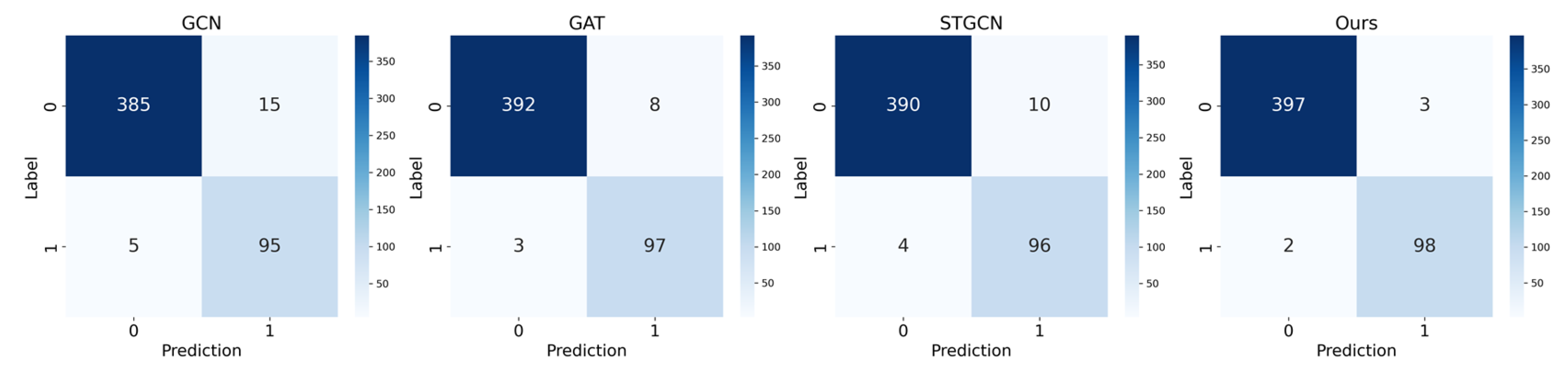
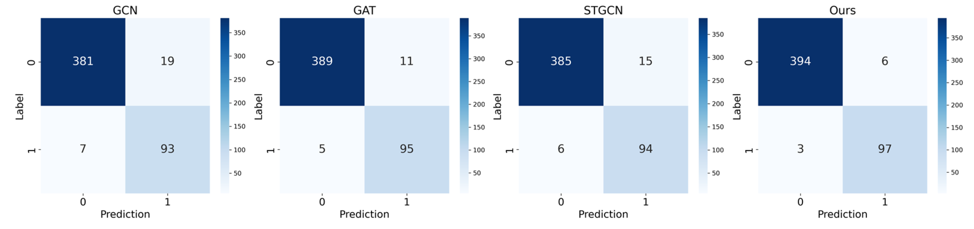
Ours	0.982	0.950	0.960	0.955	37

indicate that, in the classification task, the proposed model demonstrates significant advantages across multiple evaluation metrics. Specifically, the accuracy on the 68-node dataset reached 99.0% while the classification accuracy on the 145-bus system and the real provincial power grid system is 98.2%. In practical terms, such high accuracy means that out of every 100 potential instability events, the model can correctly identify 98 to 99, greatly reducing the risk of missed alarms in real-world operations. The confusion matrices shown in Figure 4, Figure 5 and Figure 6 further illustrate these improvements. Compared to GCN-GRU, the model achieves an average improvement of 3.7%, 1.5% compared to GAT, and 2.3% compared to STGCNs. Notably, the proposed model also shows significant enhancements in precision and recall across all datasets, with the F1 score being 9.3% higher than that of GCN-GRU, 3.7% higher than that of GAT, and 5.9% higher than that of STGCNs. The improved F1 score directly translates into a better balance between false alarms and missed detections in stability monitoring, which is crucial for maintaining grid reliability while avoiding unnecessary interventions. Moreover, by incorporating a multi-output classification network with an adaptive early exit mechanism, the proposed model significantly reduces the average inference time—reducing it by 44.6% compared to GCN-GRU, 72.8% compared to GAT, and 38.6% compared to STGCNs. In practical applications, this reduction in inference time means that the model can complete stability assessments in an average of only 37 milliseconds, well below the standard requirement of completing the task within 100 milliseconds for real-time grid monitoring and control. Compared to GCN-GRU, GAT, and STGCNs, the proposed model not only increases the accuracy by an average of 2.5% but also reduces the inference time by 52.1%. These improvements enable the model to simultaneously meet the accuracy and speed requirements of modern grid operation centers, where rapid and accurate stability assessments are crucial for maintaining grid reliability. Overall, these results fully demonstrate the comprehensive advantages of the proposed model in terms of both accuracy and efficiency, showcasing its outstanding performance.

5.4. Ablation Study

(1) Variation in model structure: to validate the effectiveness of the proposed model, which combines an STGCN backbone with a decoder and multi-exit classification network for power system transient time series data, we conducted several comparative experiments on a real provincial power grid system.

• Backbone + single-exit model (B + S): only the STGCN backbone is used, followed by a fully connected layer for classification.
• Backbone + decoder (B + D): the decoder is connected after the STGCN backbone for the reconstruction and prediction of graph data but does not include a multi-exit classifier.
• Backbone + multi-exit classification (B + M): directly connected to the multi-exit classification network after the STGCN backbone without the decoder.
• Backbone + decoder + single-exit classifier (B + D + S): the decoder and a single classifier exit are connected after the STGCN backbone.
• Ours: a decoder and a multi-exit classification network with four classifier exits are connected after the STGCN backbone, with adaptive exit selection based on confidence.

The ablation experiments, as shown in

Table 5. Impact of individual modules on model performance.

Methods	Accuracy	Prediction Error	Inference Time (ms)	Early Stopping Rate (%)
B + S	0.944	-	29	-
B + D	-	0.0145 ± 0.0040	32	-
B + M	0.974	-	31	0.798
B + D + S	0.962	0.0134 ± 0.0038	34	-
Ours	0.982	0.0127 ± 0.0033	37	0.836

, clearly demonstrate the significant contributions of each module in the proposed model. Firstly, the multi-exit classification model achieves a classification accuracy of 97.4%, representing a 3.1% improvement over the single-exit model. Secondly, the multi-task model shows noticeable improvements in both accuracy and prediction error, indicating the synergistic benefits among tasks. Specifically, the multi-task framework achieves a prediction accuracy of 98.2% and an MAE of 0.0127, both of which outperform the corresponding results from the single-task model, indicating that the joint learning of related tasks can boost their respective performances. By integrating multiple tasks with a multi-exit mechanism, the proposed model achieves substantial improvements in classification accuracy and prediction error. Moreover, 83.6% of the data are successfully processed by shallow classifiers, significantly reducing computational resource consumption. These results highlight the comprehensive advantages of the proposed model in terms of both accuracy and efficiency, further validating the effectiveness and contribution of each individual module.

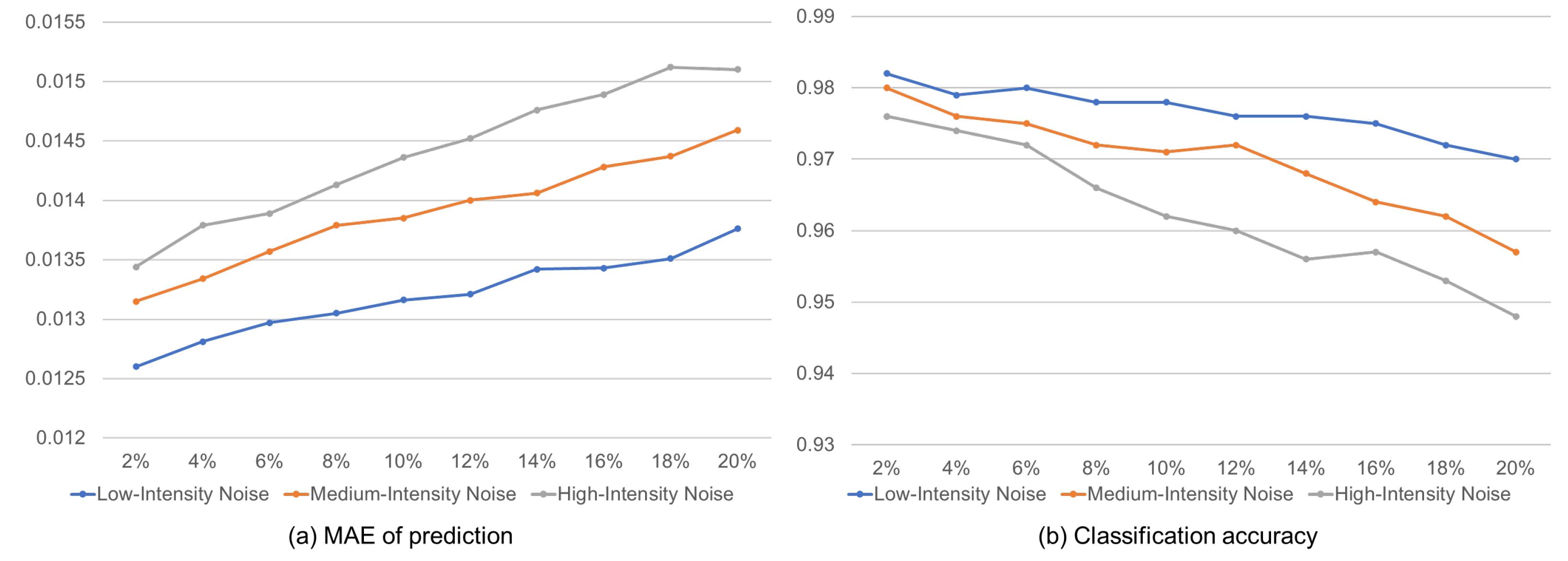
(2) Noise level: To further evaluate the robustness of the proposed model against noise interference, ablation experiments were conducted. Gaussian random noise with varying intensity and proportion was added to the transient temporal graph data of the power system to assess its impact on both graph data prediction and classification tasks. The noise settings used in the experiments are as follows:

• Noise intensity: the mean $\mu$ of the Gaussian noise was set to 0, with standard deviations $\sigma$ of 0.01, 0.05, and 0.1, corresponding to low, medium, and high levels of noise intensity, respectively.
• Noise proportion: nodes accounting for 2%, 4%, 6%, 8%, 10%, 12%, 14%, 16%, 18%, and 20% of the original data were randomly selected for noise addition, simulating various levels of noise contamination.

As shown in Figure 7, as noise intensity and noise proportion increase, the model’s MAE gradually rises, indicating a growing prediction error. When the noise proportion reaches 20% and the noise intensity is high ($\sigma$ = 0.1), the MAE reaches its peak, though it remains within an acceptable range.

The classification accuracy decreases as noise increases, and noise has a significant impact on classification performance. Under low-intensity noise conditions, even when the noise proportion reaches 20%, the model maintains 97% accuracy. However, high-intensity noise has a greater impact on classification performance, reducing the accuracy to 94.8%.

The experimental results demonstrate that the introduction of Gaussian random noise positively affects the model’s graph data prediction and classification tasks. Nonetheless, the proposed model consistently maintains a high performance even under moderate levels of noise interference. This suggests that the model possesses strong noise resistance, making it well suited for applications in power systems where noise and data contamination are present.

6. Conclusions

This paper proposes a multi-task learning framework based on STGCNs to address the growing complexity and uncertainty in modern power systems. Through comprehensive experiments conducted on standard IEEE test systems and real-world power grids, we demonstrate the framework’s superior performance in transient stability assessment and state prediction compared to conventional approaches. The key contributions encompass three main aspects: (1) effective spatiotemporal feature extraction through an ST-GCN architecture, (2) accurate state prediction enabled by a novel self-attention U-shaped residual decoder, and (3) efficient transient stability assessments achieved via an innovative multi-exit strategy. While achieving promising results, current challenges persist regarding scalability for large-scale networks and computational efficiency requirements for real-time implementation. Future research will explore advanced artificial intelligence techniques to enhance the framework’s adaptability and robustness across diverse conditions. We believe that the methods and findings in this study will drive intelligent and efficient power system monitoring and control in the era of renewable energy integration and smart grids.