Day-Ahead Net Load Forecasting for Renewable Integrated Buildings Using XGBoost

Abstract

With the large-scale adoption of photovoltaic (PV) systems as a renewable energy source, accurate long-term forecasting benefits both utilities and customers. However, developing forecasting models is challenging due to the need for high-quality training data at fine time intervals, such as 15 and 30 min resolutions. While sensors can track necessary data, careful analysis is required, particularly for PV systems, due to weather-induced variability. Well-developed forecasting models could optimize resource scheduling, reduce costs, and support grid stability. This study demonstrates the feasibility of a day-ahead net load forecasting model for a mixed-use office building. The model was developed using multi-year campus load and PV data from the University of Hawaii at Manoa. Preprocessing techniques were applied to clean and separate the data, followed by developing two decoupled models to forecast gross load demand and PV production. A weighted-average function was then incorporated to refine the final prediction. The results show that the model effectively captures day-ahead net load trends across different load shapes and weather conditions.

1. Introduction

Renewable energy has emerged as a critical factor in meeting global electricity demands and addressing climate change. According to the National Renewable Energy Laboratory (NREL), 38% of the world’s electricity in 2022 was generated by carbon-free sources, including nuclear and hydroelectric power [1]. Among these, photovoltaic (PV) systems accounted for more than half of the electricity generated, making PV the fastest-growing generation technology today [1]. One of the primary drivers of this growth has been the significant decline in costs, with the cost of PV electricity decreasing by 85% between 2010 and 2020 [2,3]. This dramatic cost reduction has enabled broader technology deployment, further reducing prices through economies of scale and creating a feedback loop of increased deployment and falling costs [3].

Many states in the United States have recently implemented amendments to achieve clean and renewable energy integration goals. Clean energy, defined as carbon-neutral generation, is governed by Clean Energy Standards (CESs), while renewable energy, derived from inexhaustible sources like solar PV, falls under Renewable Portfolio Standards (RPSs) [4]. Examples of these ambitious state targets include California, Colorado, Hawaii, and Washington, all of which aim for 100% RPS/CES compliance between 2045 and 2050 [4]. Achieving these goals requires significant advancements in the monitoring and forecasting of both gross load demand and renewable energy resources.

To further the CES and RPS goals, researchers aim to improve the accuracy of both direct and indirect net load forecasting techniques. Traditionally, the net load is determined by subtracting the gross load from behind the meter energy generation source, such as a rooftop PV system. Among the approaches available for net load forecasting, some researchers have focused on predicting net load directly from the perspective of the utility company, while others have employed indirect or decoupled forecasting methods. In the latter approach, separate models are developed to predict an infrastructure’s gross load and daily renewable energy output. In recent years, both methods have been enhanced through a combination of data preprocessing and machine learning modeling, aiming to capture the complex relationships between input and output variables.

A review of the literature indicates that popular machine learning models for load, PV, and other types of detection and forecasting include support vector machines (SVMs), neural networks, such as long short-term memory (LSTM) models, and gradient boosting, and statistical methods such as the Autoregressive Integrated Moving Average (ARIMA) and Markov chains [5,6,7,8]. Dai and Zhao [9] developed a hybrid model that combined the nonlinear prediction capabilities of an SVM with a feature parameter optimization function. When comparing this hybrid model to an mRMR-GA-SVM, BPNN, and MRMBPNN, the hybrid SVM model achieved the highest accuracy over a 24 h interval with a mean-average percent error (MAPE) score of 0.0412. Montoya and Mandal [10] examined various PV forecasting techniques, including LSTM, a feed-forward neural network using an Extreme Learning Machine (ELM), and a shallow-learning network known as the Elman Neural Network (ENN). Their research showed that when training each model on a similar database, the LSTM outperformed other models for both day-ahead and week-ahead forecasts across various seasons. Duy et al. [11] demonstrated that replacing traditional time-based features with irradiance features improved the accuracy of a recurrent LSTM model. By creating and comparing two models with similar training and test sets but different feature selections, they found a 24% increase in accuracy, achieving an MAPE score of 2.766%. Additionally, ref. [12] explored a strategy that combined a dual Direct-Recursive Hybrid (DirRec) and Multi-Input Multi-Output (MIMO) model to improve 1- to 3-year load forecast accuracy on the New South Wales network. This MIMO model forecasts each month’s total load demand, while the DirRec model predicts the peak load. When these two models were combined, they demonstrated significantly higher accuracy compared to other model types, such as ARIMA and variations in LSTM techniques, when trained on the same datasets. Ref. [13] demonstrated the use of a novel meta-heuristic algorithm to improve the maximum power point tracking (MPPT) and overall performance of a PV module. The study utilized crow electric fish search optimization (CEFSO) to create a hybrid CEFSO-MPPT model, which maximized the power output under changing weather conditions. After validation, it was shown that the CEFSO-MPPT model demonstrated greater module performance, higher efficiency, and lower computational complexity and tracking relative to existing MPPT models.

Contrary to forecasting only the load or PV, ref. [14] demonstrates the application of a Bayesian Neural Network (BNN) for direct short-term net load forecasting (STNLF). In their research, they found that utilizing a five-stage modeling process—with an emphasis on data quality assessment and input feature identification prior to the BNN—resulted in a 17.77% improvement in performance compared to more simple forecasting techniques. The test was conducted using one year’s worth of data collected from the UCY microgrid in Nicosia, Cyprus. Similarly, ref. [15] demonstrated that implementing a robust preprocessing phase, where missing data were replaced and normalized using the average power net load (PNL) from the previous two days, improved forecasting accuracy compared to prior studies that opted to remove all missing data. After preprocessing, the data were fed into an LSTM model, which achieved 97.7% accuracy when validated against a real-world Austrian dataset.

After reviewing the literature, it was determined that certain areas of net load forecasting remain underexplored. While the previously mentioned studies demonstrate advanced techniques in data preprocessing and the development of robust algorithms—particularly for load and PV forecasting—few specifically focus on direct and decoupled net load forecasting. Additionally, many studies prioritize achieving high accuracy in short-term predictions, which may not be practical when forecasting at daily or weekly timescales.

The goal of this work is to develop a decoupled day-ahead net load forecasting model that incorporates a weighted average function to blend historical load trends and weather patterns with forecasted predictions from an XGBoost model [16]. All data used in this study were sourced from a mixed-use office building located at the University of Hawaii at Manoa. The target building, John A. Burns Hall, was selected due to its existing 180 kW DC PV system and access to a 15 min resolution load and PV database. XGBoost was chosen for model development due to its ability to capture complex relationships and its strong track record in time series forecasting research.

Restating this below, the key contributions and objectives of this research are as follows:

• Demonstrating a weighted average function to blend historical load and PV trends with forecasted predictions, maximizing accuracy in day-ahead net load forecasting.
• Utilizing relevant training and validation data from a mixed-use university building.
• Implementing XGBoost as the forecasting framework, in contrast to other popular techniques such as LSTM and SVM.
• Expanding research on day-ahead net load forecasting rather than focusing solely on short-term or singular-interval forecasting.

The structure of this paper is organized into three main sections. Section 2 provides background information, including details on the gross load and PV datasets, weather data, the choice of forecasting model, the weighted-average function, and the evaluation techniques. Section 3 covers the experiments and results, detailing how the forecasting models were trained and validated, and discussing their performance against the ground truth. Finally, Section 4 presents the conclusion, summarizing the experimental results and addressing the original goals of this study.

2. Background

Section 2 outlines the sources of the gross load and PV datasets, the weather data, forecasting model selection, the implementation of a weighted-average function, and the evaluation techniques employed in this study.

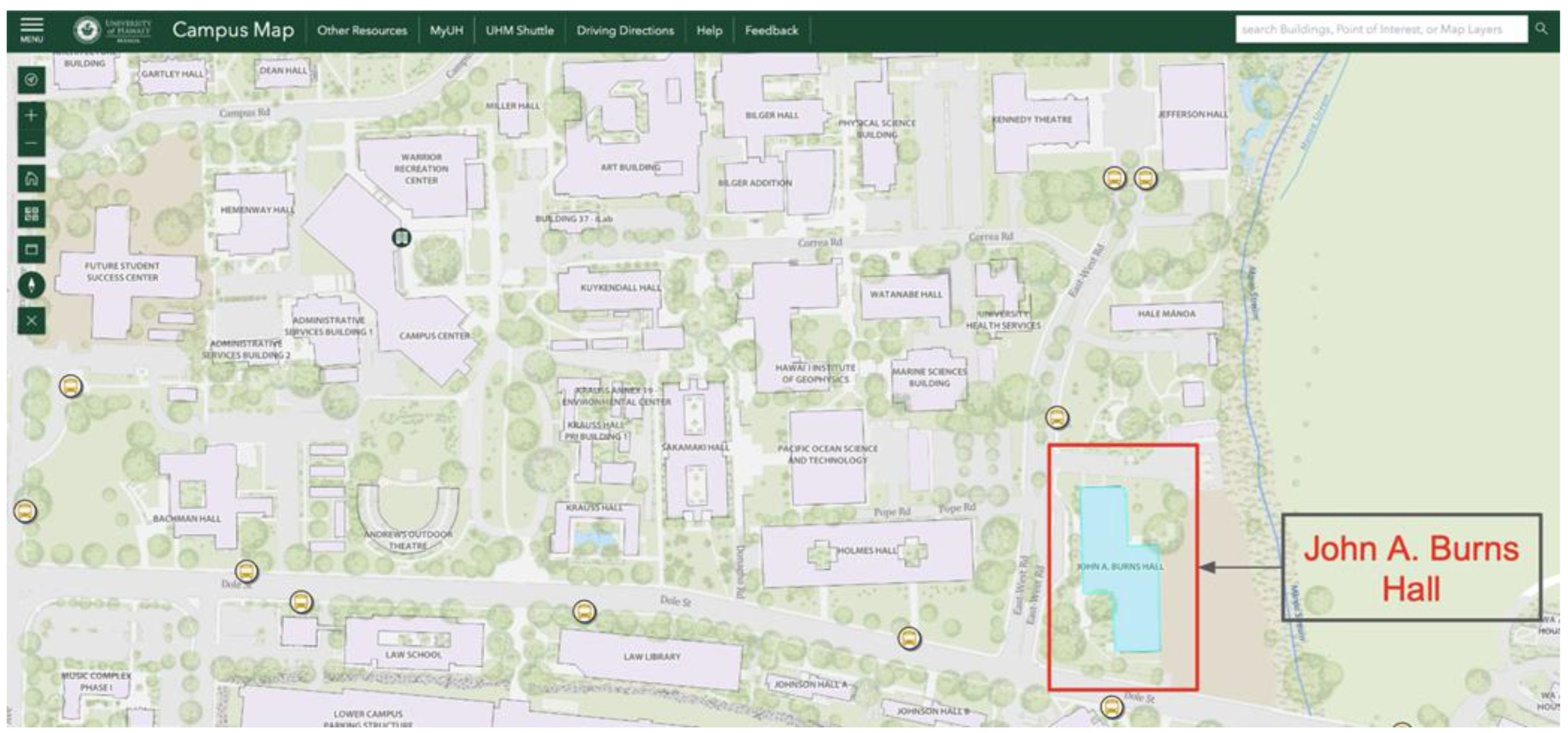
2.1. Building Load and PV Data

Access to a large, high-quality dataset is essential before conducting any experiment. Such datasets are necessary to create training sets that capture at least one year of seasonality and variation. Training data play a critical role in developing a robust, generalizable forecasting model that minimizes significant errors caused by small changes in input. The University of Hawaii provided the building load and PV data for this experiment.

The building load and PV data were collected from a multi-story, mixed-use office building on the Manoa campus of the University of Hawaii. The building contains several small multi-purpose rooms, an art exhibit, and shared spaces for the university staff’s daily use. The office building has an average load of approximately 250 kW, with data tracked from 14 June 2021 to 14 July 2023 at 15 min intervals using a Vitality load monitoring system. The rooftop solar PV system has a total capacity of 180 kW DC, with data recorded from 1 July 2021 to 18 July 2023 at 15 min intervals using a similar monitoring system. The building’s location is shown on the university map in Figure 1.

2.2. Open-Meteo Historical Weather Database

Open-Meteo is a free, open-source weather API that provides access to historical weather forecasts and recordings [17]. It achieves this by partnering with organizations such as the National Oceanic and Atmospheric Administration (NOAA) to obtain measurement data from weather stations, satellites, radar, airplanes, and buoys. The databases are updated at intervals of 1, 3, or 6 h, depending on location, to ensure users have access to accurate, direct measurement data. Open-Meteo has been assessed as a credible source for providing high-quality weather measurements, as it retrieves data directly from science-based U.S. federal agencies and other national weather services [18,19,20]. Additionally, it is an open-source platform with extensive documentation, allowing users to verify the database and its associated repositories. For this research, Open-Meteo was used to retrieve historical weather data for the university campus. The platform was selected for its wide range of available variables, including cloud coverage, solar radiation, and temperature, as well as its ease of use in compiling all required feature data. Without access to these databases, the accuracy of the PV forecasting model would be significantly impacted, as weather-based feature selection is widely recognized as a key factor in improving forecasting accuracy. Moreover, inaccurate or missing weather data would lead to a substantial drop in accuracy, as the weighted-average function and training inputs for the PV model would fail to properly reflect the ground truth output.

2.3. XGboost

XGBoost was selected as the framework for the forecasting model. Also known as extreme gradient boosting, XGBoost is a decision tree algorithm that is highly effective for classification and regression problems due to its robust learning capabilities [16]. The boosting technique is particularly advantageous for preventing overfitting, managing complex relationships within data, and supporting time-series forecasting. XGBoost has gained widespread popularity across various applications, including sales and market forecasting, industrial forecasting, and electricity consumption forecasting [21,22,23]. For this experiment, XGBoost was chosen for its strong performance capabilities and flexibility, enabling the effective handling of both gross load forecasting and PV forecasting without the need to develop two significantly distinct models.

2.4. Weighted-Average Function

The weighted-average function is a technique that has been shown to significantly enhance accuracy in both short-term gross load and PV forecasting [24,25]. This method combines the original forecast with a database generated from a historical seasonal load or PV data. By integrating these components, the technique helps to mitigate forecast outliers and promotes trends that align with the expected load and PV patterns.

A modified version of the weighted-average function was utilized in this research to accommodate the nature of decoupled net load forecasting. Two separate historical datasets were generated: one containing average building load data and the other containing average PV output data. The average building load data were calculated by categorizing historical load data into monthly groups and averaging 15 min intervals based on weekday versus weekend loads, capturing differences in usage due to the university faculty presence on weekdays. Similarly, the average PV data were categorized by month and averaged across 96 steps. However, instead of distinguishing between weekdays and weekends, the cloud coverage percentage during daylight hours was used to classify the days as cloudy or sunny. On sunny days, a mound-shaped PV output with minimal variation was expected, whereas cloudy days were associated with a reduced peak amplitude and increased variability.

Next, the forecast date and outputs from each trained XGBoost model were used as inputs for the weighted-average function. The function retrieves historical load and PV data from their respective data frames based on the forecast date and weather type. Subsequently, an alpha coefficient is assigned to the forecasted output, while a beta coefficient is assigned to the historically averaged data frame. The alpha and beta coefficients must be set between zero and one, with their sum equaling one. The purpose of these coefficients is to blend the two datasets into a specific ratio to generate a final prediction. A higher alpha value increases the influence of the forecasted XGBoost output, whereas a larger beta coefficient places greater emphasis on historical trends rather than the forecast model. Three alpha–beta coefficient ratios were tested as follows: (0.25, 0.75), (0.5, 0.5), and (0.75, 0.25). Among these, the (0.5, 0.5) ratio yielded the highest test accuracy. This balanced coefficient ratio effectively incorporated historical influences, capturing both load and PV patterns while also allowing for sufficient variation to account for load spikes and weather changes. Equations (1)–(3) illustrate how the initial forecasts and historical values were combined to produce a hybrid net load forecast.

GLF = (α · Initial LF) + (β · Avg Historic Load)

(1)

where “GLF” is the gross load forecast; “ILF” is the initial load forecast from the XGBoost model; and “Avg Historic Load” is the average historic load for the specific month and day of the week.

PV Forecast = (α · Initial PVF) + (β · Avg Historic PV)

(2)

where “initial PVF” is the initial PV forecast from the XGBoost model, and “Avg Historic PV” is the average historic PV for the specific month and weather type.

Net Load Forecast = GLF − PV Forecast

(3)

It is important to note that the alpha and beta coefficients for the gross load forecast and PV forecast do not need to be identical, as they pertain to two separate decoupled models. Figure 2 provides a detailed explanation of the forecasting model and the weighted-average function.

2.5. Evaluation

To assess the performance of the training and validation sets, several key performance metrics were utilized. Equations (4)–(6) define the root-mean-squared error (RMSE), mean absolute error (MAE), and mean absolute percentage error (MAPE), respectively. These metrics provide a quantitative measure of forecasting accuracy by evaluating the deviations between predicted and actual values, ensuring the reliability and effectiveness of the developed model.

$$RMSE=\sqrt{{\displaystyle \frac{1}{n}}{\sum }_{i=1}^n{({GroundTruth}_i-{Forecast}_i)}^2}$$

(4)

$$MAE={\displaystyle \frac{1}{n}}{\sum }_{i=1}^n\left|{GroundTruth}_i-{Forecast}_i\right|$$

(5)

$$MAPE={\displaystyle \frac{100}{n}}{\sum }_{\ddot{L}=1}^n\left|{\displaystyle \frac{Ground{Truth}_i-{Forecast}_i}{Ground{Truth}_i}}\right|$$

(6)

Each equation’s performance is validated for a complete forecast day at a 15 min resolution, meaning each day consists of n = 96 steps. RMSE was chosen because it evaluates the forecast against the ground truth while preserving the original unit reference. MAE was included for its ability to maintain the unit reference and provide the average absolute difference between the forecast and the ground truth. MAPE was also utilized, as it offers similar insights to MAE but expresses the difference as a percentage, allowing for better interpretability.

3. Experiment and Results

Section 3 outlines the training process of the forecasting models and presents the case study along with the accompanying results.

3.1. Training Hyperparameters and Dataset

Basic data preprocessing was conducted to train the gross load and PV forecasting models. Since both models share a date range from 1 July 2021 to 14 July 2023, we split the training and test data on 1 January 2023. This provided a sufficiently large training set to capture at least one year of variation while reserving a validation test set of over six months.

Across both load and PV datasets, no outages or data gaps longer than six hours were observed. When gaps in the recorded load data occurred, missing values were replaced with average data from the previous two weeks of similar weekday and weekend day types. For missing PV data, average values from the same hour under comparable sunny or cloudy weather conditions were used as replacements. Care was taken to ensure that the imputed values closely mimicked the expected load and PV patterns under similar conditions for both profiles. Additionally, outlier data—such as values exceeding the maximum expected outputs or sudden drops in recorded load and PV data—were adjusted by extrapolating values from neighboring time intervals to prevent abrupt shifts and disruptions in training.

Basic hyperparameter tuning was also performed on the XGBoost model. Hyperparameter tuning is essential for improving model performance while also preventing overfitting. The number of estimators, learning rate, and maximum depth were monitored and manually adjusted to optimize the performance. Estimators represent the number of trees available to the model for characterizing the training data. The learning rate defines the step size used to adjust feature weights from each tree. Max depth specifies how deep each estimator or tree can traverse to establish further connections within the data. The number of estimators and max depth share an inverse relationship—where a large number of estimators combined with a deep depth limit can lead to severe overfitting. Tuning the learning rate is also crucial, as setting it too low or too high can prevent the model from generalizing unseen data effectively.

Table 1. Hyperparameters for gross load and pv forecast.

Hyperparameter	Gross Load Forecast	PV Forecast
Estimators	200	250
Learning Rate	0.25	0.5
Max Depth	6	6

presents the exact hyperparameter values used for tuning the XGBoost model.

3.2. Case Study

As described in the previous section, the original dataset was split on 1 January 2023, creating a validation test set spanning 1 January 2023 to 14 July 2023. This period captures a diverse range of day types and weather conditions. For this experiment, two specific days were selected to represent sunny and cloudy weather scenarios and weekday and weekend load profiles. Figure 3, Figure 4 and Figure 5 present the overlapped ground truth versus forecast plots for gross load, PV production, and net load on 5 March 2023. In each figure, the ground truth is represented by a dashed green line, while the forecasted output is shown as a solid red line. This date was classified as sunny due to low cloud coverage during daylight hours, and the date fell on a weekend (Sunday). The 31 March 2023 was chosen as a secondary example. Within the same month, this date exhibited cloudy weather characteristics and corresponded to a weekday (Friday). Figure 6 presents its net load forecast plot.

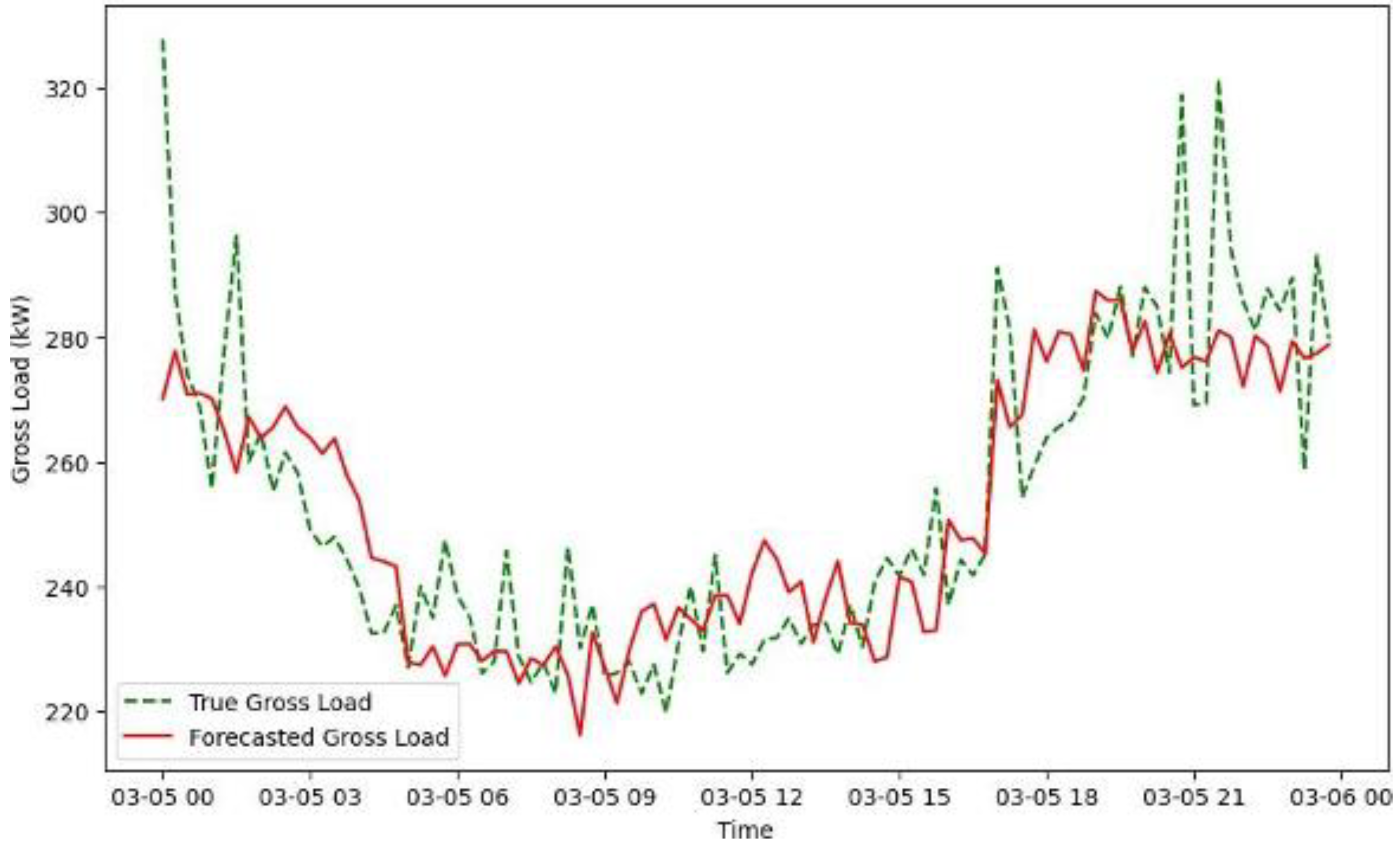
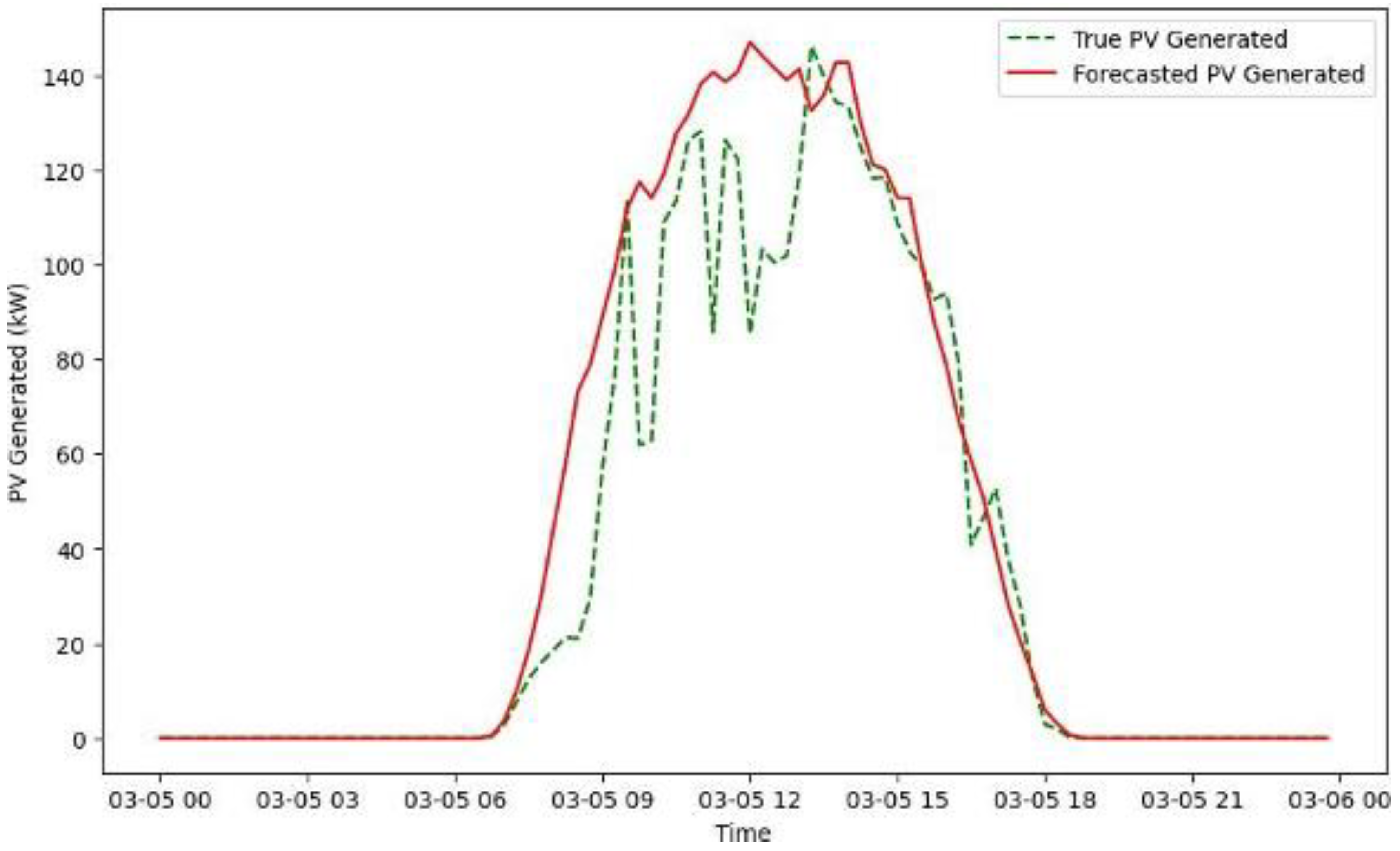
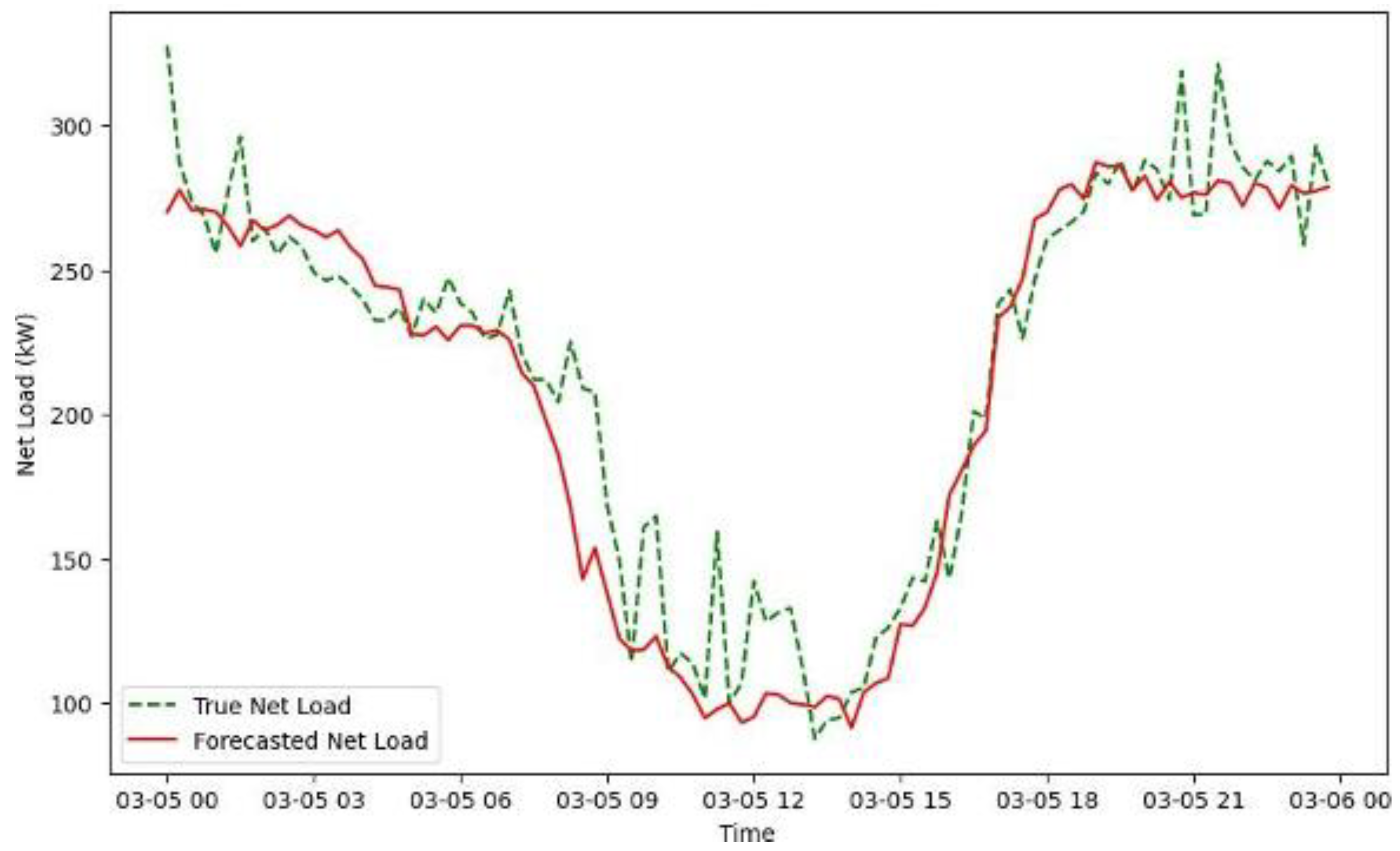
3.3. Results and Analysis

The 5 March 2023 was selected as the first evaluation day. The gross load forecast, shown in Figure 3, exhibits a load curve with peaks at the beginning and end of the day and a slight dip in the load during midday. Significant variation is present throughout the curve, causing fluctuations, with the largest deviations occurring at the start and end of the day. When comparing the gross load forecast to the ground truth, the forecast effectively captures the overall characteristics of the load curve. However, while the forecast includes interval-to-interval variations, it does not fully replicate the exact amplitudes of these variations on a per-interval basis. The gross load forecast achieved an RMSE of 13.93, an MAE of 10.40, and an MAPE of 0.04.

Figure 4 presents the overlapped PV ground truth and forecast plot for the same day (5 March). The ground truth and the forecast exhibited the expected mound-shaped curve, with peaks occurring at midday and declines before 6:00 a.m. and after 6:00 p.m. The PV forecasting model successfully captured the overall trend with minor variations but struggled to account for the amplitude changes caused by sudden weather variations, resulting in overshooting during midday hours. Due to this overshooting, the model achieved an RMSE of 25.80, an MAE of 18.80, and an MAPE of 0.39. Figure 5 compares the net load ground truth with the forecasted net load. Since the forecasted net load is derived from the difference between the forecasted gross load and PV output, the forecast closely follows the overall trend but exhibits both overshooting and undershooting throughout the period. Most undershooting occurs at the tails of the plot, before and after peak sun hours, as observed in Figure 3. Overshooting PV production during midday, caused by weather variability, resulting in a lower-than-expected net load. Overall, the net load forecast achieved an RMSE of 21.13, an MAE of 15.24, and an MAPE of 0.08. All evaluation metrics for Figure 3, Figure 4 and Figure 5 are summarized in

Table 2. March 5th forecast accuracy.

Metric	RMSE [kW]	MAE [kW]	MAPE
Gross Load Forecast	13.93	10.40	0.04
PV Forecast	25.80	18.80	0.39
Net Load Forecast	21.13	15.24	0.09

.

Figure 6 visualizes the true versus forecasted net load for 31 March 2023. This day was selected because it represented a cloudy weather pattern and weekday load characteristics, in contrast to 5 March, which was a sunny weekday. Similarly to 5 March, the net load curve on this day exhibits a duck shape, with peaks at the beginning and end of the day with a midday trough. However, because March 31 was cloudy, the midday trough displays a higher net load amplitude and greater interval-to-interval variation. Examining the overlap between the forecast and ground truth, this model effectively captures the general trend of the net load but struggles to represent the scale of the variations. The net load was over-forecasted from 6:00 a.m. to 12:00 p.m., while from 2:00 p.m. to 6:00 p.m., it was under-forecasted. The cause of these differences was due to the PV forecasting model being unable to capture the scale of each variation due to shifts in the cloud coverage percentage despite remaining cloudy overall. The overall accuracy of the model for cloudy days is summarized in

Table 3. March 31st forecast accuracy.

Metric	RMSE [kW]	MAE [kW]	MAPE
Gross Load Forecast	10.63	8.41	0.04
PV Forecast	34.31	27.00	0.94
Net Load Forecast	23.57	16.54	0.08

, with the net load forecast achieving an RMSE of 22.02, an MAE of 16.56, and an MAPE of 0.09.

3.4. Discussion

Figure 5 and Figure 6 present overlapped plots of the ground truth versus forecasted net load when applying a weighted-average function to a day-ahead net load forecasting model. In both cases, the forecast closely followed the overall trend of the true net load but struggled to capture midday variations, primarily due to weather fluctuations, while remaining within the general sunny or cloudy classifications. As a result, both test cases exhibited periods of overestimation and underestimation during daylight hours, leading to higher overall RMSE, MAE, and MAPE scores.

To enhance the performance of real-world applications, improvements to the PV forecasting model are necessary. Potential mitigation strategies include expanding the training and historical datasets to incorporate more recent weather trends. Another possible improvement involves refining the classification of cloudy and sunny weather conditions by creating more targeted time windows. Implementing shorter 4–6 h windows for weather classification, rather than categorizing the entire daylight period under a single weather type, could enhance the model’s accuracy. Additionally, adjusting the hyperparameter tuning of the PV forecasting model to strengthen connections with the training data could further improve performance. Further experimentation with modifying the alpha–beta coefficient ratio to better capture historical trends under similar weather conditions may also yield slight performance gains. Finally, future work should explore tuning, developing, and comparing alternative machine learning models such as LSTM, ARIMA, and neural networks (NNs) in combination with the weighted-average function to determine whether a model change can lead to improved forecasting accuracy.

4. Conclusions

With the growing expansion of renewable energy resources, accurate long-term net load forecasting is becoming increasingly critical for utility companies and customers. This research demonstrates the viability of a day-ahead net load forecasting model using XGBoost, coupled with a weighted-average function, across various day-type scenarios. When tested on a sunny weekend, the model produced an RMSE of 13.93 kW for gross load, 34.31 kW for PV, and 23.57 kW for the forecasted net load. This resulted in an MAPE score of 0.09. For cloudy weekday scenarios, the model had an RMSE of 10.63 kW for gross load, 34.31 kW for PV, and 23.57 kW for the forecasted net load, resulting in an MAPE of 0.08. Comparing Figure 5 and Figure 6, both scenarios demonstrated a strong alignment with the true net load, with key differences concentrated around midday fluctuations caused by PV forecast overshooting and undershooting. With further improvements to the PV forecasting model—such as updates to modeling data, refinements in daily weather classification, and experimentation with alternative machine learning models such as LSTM, ARIMA, and neural networks (NNs)—its performance may be enhanced, leading to greater accuracy in net load forecasting. Future work should continue exploring these potential improvements to further optimize performance and advance toward real-world implementation.

References

1. Drevers, H. At a Glance: How Renewable Energy Is Transforming the Global Electricity Supply. National Renewable Energy Laboratory. 2023. Available online: https://www.nrel.gov/news/program/2023/how-renewable-energy-is-transforming-the-global-electricity-supply.html (accessed on 1 March 2025).
2. News Release: Next Decade Decisive for PV Growth on the Path to 2050. National Renewable Energy Laboratory. 2023. Available online: https://www.nrel.gov/news/press/2023/news-release-next-decade-decisive-for-pv-growth-on-the-path-to-2050.html (accessed on 1 March 2025).
3. Renewable Power Generation Costs in 2020. International Renewable Energy Agency. 2021. Available online: https://www.irena.org/publications/2021/Jun/Renewable-Power-Costs-in-2020 (accessed on 1 March 2025).
4. State Renewable Portfolio Standards and Goals. National Conference of State Legislatures. 2021. Available online: https://www.ncsl.org/energy/state-renewable-portfolio-standards-and-goals (accessed on 1 March 2025).
5. Mamun, A.A.; Sohel, M.; Mohammad, N.; Haque Sunny, M.S.; Dipta, D.R.; Hossain, E. A Comprehensive Review of the Load Forecasting Techniques Using Single and Hybrid Predictive Models. IEEE Access 2020, 8, 134911–134939. [Google Scholar] [CrossRef]
6. Barhmi, K.; Heynen, C.; Golroodbari, S.; van Sark, W. A Review of Solar Forecasting Techniques and the Role of Artificial Intelligence. Solar 2024, 4, 99–135. [Google Scholar] [CrossRef]
7. Hong, T.; Wang, P. Artificial Intelligence for Load Forecasting: History, Illusions, and Opportunities. IEEE Power Energy Mag. 2022, 20, 14–23. [Google Scholar] [CrossRef]
8. Kagade, R.B.; Vijayaraj, N. Intrusion detection via optimal tuned LSTM model with trust and risk level evaluation. Int. J. Bio-Inspired Comput. 2024, 23, 39–52. [Google Scholar] [CrossRef]
9. Dai, Y.; Zhao, P. A Hybrid Load Forecasting Model Based on Support Vector Machine with Intelligent Methods for Feature Selection and Parameter Optimization. Appl. Energy 2020, 279, 115332. [Google Scholar] [CrossRef]
10. Montoya, A.Y.; Mandal, P. Day-Ahead and Week-Ahead Solar PV Power Forecasting Using Deep Learning Neural Networks. In Proceedings of the 2022 North American Power Symposium (NAPS), Salt Lake City, UT, USA, 9–11 October 2022; pp. 1–6. [Google Scholar] [CrossRef]
11. Bui Duy, L.; Nguyen Quang, N.; Doan Van, B.; Riva Sanseverino, E.; Tran Thi Tu, Q.; Le Thi Thuy, H.; Le Quang, S.; Le Cong, T.; Cu Thi Thanh, H. Refining Long Short-Term Memory Neural Network Input Parameters for Enhanced Solar Power Forecasting. Energies 2024, 17, 4174. [Google Scholar] [CrossRef]
12. Zhang, T.; Wang, Y.; Li, X.; Chen, J.; Liu, H.; Zhao, Q.; Xu, Z. Long-Term Energy and Peak Power Demand Forecasting Based on Sequential-XGBoost. IEEE Trans. Power Syst. 2024, 39, 3088–3104. [Google Scholar] [CrossRef]
13. Sebi, N.P. Intelligent MPPT for photovoltaic panels on grid-connected inverter system using hybrid meta-heuristic algorithm. Int. J. Bio-Inspired Comput. 2024, 23, 245–256. [Google Scholar] [CrossRef]
14. Tziolis, G.; Livera, A.; Montes-Romero, J.; Theocharides, S.; Makrides, G.; Georghiou, G.E. Direct Short-Term Net Load Forecasting Based on Machine Learning Principles for Solar-Integrated Microgrids. IEEE Access 2023, 11, 102038–102049. [Google Scholar] [CrossRef]
15. Mokarram, M.J.; Rashiditabar, R.; Gitizadeh, M.; Aghaei, J. Net Load Forecasting of Renewable Energy Systems Using Multi-Input LSTM Fuzzy and Discrete Wavelet Transform. Energy 2023, 275, 127425. [Google Scholar] [CrossRef]
16. XGBoost Documentation—Xgboost 2.1.3 Documentation. Available online: https://xgboost.readthedocs.io/en/stable/ (accessed on 14 March 2025).
17. Zippenfenig, P. Open-Meteo.com Weather API [Computer Software]. Zenodo 2023. [Google Scholar] [CrossRef]
18. Hersbach, H.; Bell, B.; Berrisford, P.; Biavati, G.; Horányi, A.; Muñoz Sabater, J.; Nicolas, J.; Peubey, C.; Radu, R.; Rozum, I.; et al. ERA5 Hourly Data on Single Levels from 1940 to Present [Data Set]. ECMWF 2023. [Google Scholar] [CrossRef]
19. Muñoz Sabater, J. ERA5-Land Hourly Data from 2001 to Present [Data Set]. ECMWF 2019. [Google Scholar] [CrossRef]
20. Schimanke, S.; Ridal, M.; Le Moigne, P.; Berggren, L.; Undén, P.; Randriamampianina, R.; Andrea, U.; Bazile, E.; Bertelsen, A.; Brousseau, P.; et al. CERRA Subdaily Regional Reanalysis Data for Europe on Single Levels from 1984 to Present [Data Set]. ECMWF 2021. [Google Scholar] [CrossRef]
21. Dairu, X.; Shilong, Z. Machine Learning Model for Sales Forecasting by Using XGBoost. In Proceedings of the 2021 IEEE International Conference on Consumer Electronics and Computer Engineering (ICCECE), Guangzhou, China, 15–17 January 2021; pp. 480–483. [Google Scholar] [CrossRef]
22. Zhai, N.; Yao, P.; Zhou, X. Multivariate Time Series Forecast in Industrial Process Based on XGBoost and GRU. In Proceedings of the 2020 IEEE 9th Joint International Information Technology and Artificial Intelligence Conference (ITAIC), Chongqing, China, 11–13 December 2020; pp. 1397–1400. [Google Scholar] [CrossRef]
23. Dong, D.; Wen, F.; Zhang, Y.; Qiu, W. Application of XGBoost in Electricity Consumption Prediction. In Proceedings of the 2023 IEEE 3rd International Conference on Electronic Technology, Communication and Information (ICETCI), Changchun, China, 26–28 May 2023; pp. 1260–1264. [Google Scholar] [CrossRef]
24. Pramanik, A.S.; Sepasi, S.; Nguyen, T.L.; Roose, L. An Ensemble-Based Approach for Short-Term Load Forecasting for Buildings with High Proportion of Renewable Energy Sources. Energy Build. 2024, 308, 113996. [Google Scholar] [CrossRef]
25. Sepasi, S.; Reihani, E.; Howlader, A.M.; Roose, L.R.; Matsuura, M.M. Very Short-Term Load Forecasting of a Distribution System with High PV Penetration. Renew. Energy 2017, 106, 142–148. [Google Scholar] [CrossRef]
Figure 1. University of Hawaii map displaying John A. Burns Hall.
Energies 18 01518 g001
Figure 2. Block diagram of forecasting model and weighted-average function.
Energies 18 01518 g002
Figure 3. Comparison of true vs. forecasted gross load for weekend load type (5 March 2023).
Energies 18 01518 g003
Figure 4. Comparison of true vs. forecasted PV production for sunny weather characteristics (5 March 2023).
Energies 18 01518 g004
Figure 5. Comparison of true vs. forecasted net load for weekend load type and sunny weather characteristics (5 March 2023).
Energies 18 01518 g005
Figure 6. Comparison of true vs. forecasted net load for weekday load type and cloudy weather characteristics (31 March 2023).
Energies 18 01518 g006