A Multi-Variable Coupled Control Strategy Based on a Deep Deterministic Policy Gradient Reinforcement Learning Algorithm for a Small Pressurized Water Reactor

Abstract

The reactor system has multivariate, nonlinear, and strongly coupled dynamic characteristics, which puts high demands on the robustness, real-time demand, and accuracy of the control strategy. Conventional control approaches depend on the mathematical model of the system being controlled, making it challenging to handle the reactor system’s dynamic complexity and uncertainties. This paper proposes a multi-variable coupled control strategy for a nuclear reactor steam supply system based on a Deep Deterministic Policy Gradient reinforcement learning algorithm, designs and trains a multi-variable coupled intelligent controller to simultaneously realize the coordinated control of multiple parameters, such as the reactor power, average coolant temperature, steam pressure, etc., and performs a simulation validation of the control strategy under the typical transient variable load working conditions. Simulation results show that the reinforcement learning control effect is better than the PID control effect under a ±10% FP step variable load condition, a linear variable load condition, and a load dumping condition, and that the reactor power overshooting amount and regulation time, the maximum deviation of the coolant average temperature, the steam pressure, the pressure of pressurizer and relative liquid level, and the regulation time are improved by at least 15.5% compared with the traditional control method. Therefore, this study offers a theoretical framework for utilizing reinforcement learning in the field of nuclear reactor control.

1. Introduction

As a key piece of equipment in a modern energy facility, the control system of a nuclear reactor needs to ensure the stability, safety, and efficiency of the reactor in an extremely complex environment. Reactor control systems face extremely high precision requirements, as fluctuations in key parameters such as temperature and power can have a significant impact on system operation. For example, the power and temperature control of a nuclear reactor require not only precision and stability but also fast response to instantaneous changes. Such a high real-time demand often requires the control system to be able to adjust the control strategy in milliseconds or even shorter to cope with rapid fluctuations in the system state. In addition, certain perturbations may exist in the operating environment of a nuclear reactor, making it necessary for the control system to be highly robust to extreme and unexpected conditions. Consequently, the development of reactor control systems remains a key focus area within nuclear engineering research.

Early studies in nuclear reactor control primarily focused on classical methods, with Proportional–Integral–Derivative (PID) controllers being widely employed by researchers for system design, including power regulation, pressurizer pressure, level control, and steam generator feedwater control [1]. As an advancement over conventional PID methods, the fractional-order PID (FOPID) controller [2,3] has seen ongoing development on nuclear reactor control because of its superior flexibility and robustness relative to traditional PID approaches.

Gradually, the advancement of control theory and the widespread adoption of digital control systems have enabled the application of sophisticated control methods, including optimal control, predictive control in modern control technologies, and intelligent approaches like fuzzy control [4] and neural network control, to the design and simulation of nuclear power plant systems. For example, a robust controller for reactor core power has been developed using the Quantitative Feedback Theory (QFT) [5], sliding mode control [6], the H∞ output feedback control theory, and the linear matrix inequality solving method [7]. There are also scholars designing robust controllers for the pressurized water reactor core Linear Quadratic Gaussian with Loop Transfer Recovery (LQG/LTR) methodology, which is suitable for load tracking control [8,9]. To achieve broad load tracking capabilities in nuclear reactor systems, some other scholars have utilized advanced and intelligent control theories for the control of the reactor system. For example, the model predictive control theory has been integrated into space reactor control [10], and its principles have been utilized to develop a wide-range load tracking controller [11,12]. However, nuclear reactors are highly nonlinear and strongly coupled systems, and for the multiple-input and multiple-output cases and the coupling effect between variables, traditional control methods usually adopt the idea of decoupling control, but it is difficult to realize complete decoupling of the actual object, and thus a more ideal control effect cannot be achieved. The limitations of these methods in reactor control make the design of more intelligent and adaptable control methods an urgent technical challenge.

With the continuous progress of artificial intelligence technology, reinforcement learning (RL) has gradually become an emerging method for solving complex control problems [13,14]. Reinforcement learning gradually learns the optimal control strategy by trial and error through the interaction of intelligence in the environment, which does not rely on precise physical models and can show strong adaptive ability in complex systems. Especially when facing complex nonlinear and high-dimensional-state spaces, the advantages of reinforcement learning become more and more obvious. Reinforcement learning has shown significant potential in the complex domain of reactor control systems, making it a prominent area of study in recent years [15,16,17]. In nuclear engineering, this approach is primarily implemented in two distinct manners. The first involves integrating reinforcement learning with conventional PID control techniques, where it is utilized to finetune PID parameters. For instance, Zhang [18] introduced a method for optimizing control objectives using deep reinforcement learning, dynamically adjusting PID controller settings to enhance the thermal power response and steam outlet temperature in nuclear reactor steam supply systems. The second method uses reinforcement learning intelligence directly as a controller. Li [19] explored the application of deep reinforcement learning in managing both the reactor power and steam generator water level, utilizing the Deep Deterministic Policy Gradient (DDPG) algorithm to facilitate interactive learning and problem solving within the reactor’s coordinated control framework. While these studies have primarily addressed individual control systems within reactors, further investigation is required to develop reinforcement-learning-based strategies for managing multiple interconnected objectives in reactor systems.

This study introduces a novel approach utilizing reinforcement learning to realize the multi-variable coupling control in the steam supply systems of nuclear reactors, which adopts the idea of holistic design, regards the reactor system as an organic whole with multiple inputs and multiple outputs, and utilizes artificial intelligence technology based on the DDPG reinforcement learning algorithm to design the system’s multi-variable coupling intelligent controller. At the same time, it realizes the key parameters of the reactor power, the average temperature of the coolant, and the steam pressure. Section 2 introduces the modeling of the nuclear reactor steam supply system, Section 3 describes the design and training method of the reinforcement learning agents, Section 4 carries out the simulation and analyses, and Section 5 is the conclusion.

2. Modeling of Nuclear Steam Supply System

This research focuses on the nuclear steam supply system (NSSS) of a small pressurized water reactor (SPWR), based on which a simulation model is developed and a reinforcement learning agent is designed and trained. The NSSS of an SPWR nuclear power plant includes key elements like the reactor core, pressurizer, once-through steam generator (OTSG), and associated control systems. The reference parameters for this study were obtained from publicly accessible literatures [20,21,22,23,24]. Where specific data were unavailable, designs from other reactor types are referenced.

2.1. Core Modeling

The core thermal and physical models are incorporated into the reactor model. A point reactor model, utilizing a one-group delayed neutron approach, serves as the reactor physical model, and the dynamics counterpart is based on one-group delayed neutrons.

$$\left\{\begin{array}{l}{\displaystyle \frac{dn}{dt}}={\displaystyle \frac{\rho -\beta }{\Lambda }}n+\lambda C\\ {\displaystyle \frac{dC}{dt}}={\displaystyle \frac{\beta }{\Lambda }}n-\lambda C\end{array}\right.$$

(1)

where n represents the neutron density, m⁻³; C denotes the precursor nucleus density, m⁻³; ρ stands for the total reactivity; Λ indicates the neutron generation time, s; $\beta$ is the total share of delayed neutrons; and λ is the one-group delayed neutron decay constant, s⁻¹.

In the core thermal model, the Mann model [25] is employed, where one fuel element corresponds to two coolant nodes. The energy conservation equations for the fuel node and the two coolant nodes are

$$\left\{\begin{array}{l}{\mu }_f{\displaystyle \frac{d{T}_f}{dt}}={\displaystyle \frac{f{P}_0}{100}}{n}_r-\Omega (T_f-T_{c1})\\ {\displaystyle \frac{{\mu }_c}{2}}{\displaystyle \frac{d{T}_{c1}}{dt}}={\displaystyle \frac{1}{2}}\left[{\displaystyle \frac{(1-f)P_0}{100}}{n}_r+\Omega (T_f-T_{c1})\right]+W_c{C}_{p,c}(T_{lp}-T_{c1})\\ {\displaystyle \frac{{\mu }_c}{2}}{\displaystyle \frac{d{T}_{co}}{dt}}={\displaystyle \frac{1}{2}}\left[{\displaystyle \frac{(1-f)P_0}{100}}{n}_r+\Omega (T_f-T_{c1})\right]+W_c{C}_{p,c}(T_{c1}-T_{co})\end{array}\right.$$

(2)

where $T_f$ represents the average fuel temperature, °C; $T_{c1}$ denotes the average core coolant temperature, °C; $T_{co}$ indicates the core outlet coolant temperature, °C; $T_{lp}$ represents the core inlet coolant temperature, i.e., the lower chamber outlet temperature, °C; $P_0$ stand for the full power value of the reactor, W; ${\mu }_f$ denotes the total heat capacity of the core fuel, ${\mu }_f=m_f{C}_{p,f}$, J·°C⁻¹; ${\mu }_c$ represents the total heat capacity of the core coolant, ${\mu }_c=m_c{C}_{p,c}$, J·°C⁻¹; $f$ is the share of heat generated in the fuel in total power; $\Omega$ represents the heat transfer coefficient between the fuel and coolant, W·°C⁻¹; $W_c$ denotes the core coolant flow rate, kg·s⁻¹; $C_{p,f}$ indicates the constant-pressure specific heat capacity, J·(kg·°C)⁻¹; and $C_{p,c}$ stands for the constant-pressure specific heat capacity of the core coolant, J·(kg·°C)⁻¹.

In this paper, from the perspective of reactor control optimization, reactivity changes are mainly caused by control rods and reactivity feedback. Therefore, in this paper, the overall reactivity in the reactor is influenced by two factors, the reactivity introduced by control rods and the negative feedback effects of moderator temperature and fuel temperature.

$$\rho ={10}^{-5}{\rho }_r+{\alpha }_f\left(T_f-T_{f0}\right)+{\displaystyle \frac{{\alpha }_c}{2}}\left[\left(T_{c1}+T_{co}\right)-\left(T_{c10}+T_{co0}\right)\right]$$

(3)

where ${\rho }_r$ represents the reactivity introduced by the control rods, and the value of the control rod integral varies nonlinearly according to the proposed rod position and is correlated with the lifetime, pcm; ${\alpha }_f$ denotes the fuel reactivity temperature coefficient, pcm·°C⁻¹; ${\alpha }_c$ is the coolant reactivity temperature coefficient, pcm·°C⁻¹; $T_{f0}$ indicates the initial temperature of $T_f$, °C; $T_{c10}$ stands for the initial temperature of $T_{c1}$, °C; and $T_{co0}$ represents the initial temperature of $T_{co}$, °C.

2.2. OTSG Modeling

The OTSG model includes the equipment model of the OTSG and the main steam system model. By assuming uniform heat transfer processes across all spiral pipes, a single spiral pipe is used as the representative heat transfer channel for modeling. Key assumptions made in the modeling process are as follows:

(1)

Identical flow rates and heat transfer capacities for all spiral tubes;

(2)

Fluid dynamics are modeled one-dimensionally along the main flow direction, with radial secondary flow effects incorporated through correction coefficients for heat transfer and pressure drop calculations;

(3)

The axial thermal conductivity of the working material and tube walls on both primary and secondary sides is neglected, along with external heat dissipation from the steam generator;

(4)

The primary-side fluid is treated as the average heat transfer channel, consistent across all spiral tubes, with the assumption of incompressibility and uniform pressure throughout;

(5)

Thermodynamic equilibrium is always maintained between the vapor and liquid phases in the two-phase region, ignoring the phenomenon of subcooling and boiling.

In this paper, multiple control bodies are divided within the OTSG (Illustrated in Figure 1). The secondary side of the superheating zone is partitioned into 3 control bodies (SFSL1, SFSL2, and SFSL3), the secondary side of the two-phase zone is segmented into 2 control bodies (SFBL1 and SFBL2), and the secondary side of the subcooling zone fluid is divided into 2 control bodies (SFCL1 and SFCL2). Accordingly, the primary side of the fluid and the metal tube wall are partitioned into 7 control bodies (PRL1, PRL2, PRL3, PRL4, PRL5, PRL6, and PRL7).

According to [26], the OTSG’s nonlinear dynamic model is developed using the lumped-parameter method, incorporating fundamental conservation equations for mass, momentum, and energy, with movable boundaries.

For the main steam system’s dynamic model, it is assumed that the steam flowing into the steam bus from each steam generator has the same flow rate and physical properties. Based on the division of control bodies in the OTSG model, Equations (4)–(6) are separately derived in the principles of mass, energy, and momentum conservations.

$$V_h{\displaystyle \frac{d{\rho }_h}{dt}}=2W_{s1}-(W_T+W_D)$$

(4)

$$V_h{\displaystyle \frac{d({\rho }_h{h}_h)}{dt}}-V_h{\displaystyle \frac{d{P}_h}{dt}}=2W_{s1}{h}_{s1}-(W_T+W_D)h_h$$

(5)

$${\displaystyle \frac{L_h}{A_h}}{\displaystyle \frac{d{W}_{s1}}{dt}}=P_{s1}-P_h-k_f{\displaystyle \frac{W_{s1}\left|W_{s1}\right|}{2{\rho }_h}}+{\rho }_{h}g\Delta H_h$$

(6)

where V_h represents the total volume of the main steam system, m³; ρ_h denotes the density of the main steam, kg·m⁻³; h_h indicates the specific enthalpy of the main steam, J·kg⁻¹; P_h stands for the pressure of the main steam, Pa; W_T represents the turbine inlet steam flow, kg·s⁻¹; W_D is the side exhaust steam flow, kg·s⁻¹; W_s1 is the steam flow on the secondary side of the SG, kg·s⁻¹; h_s1 denotes the specific enthalpy of the steam on the secondary side of the SG, kg·s⁻¹; ∆H_h is height difference between the steam nozzle to the main steam bus, m; and k_f is the equivalent resistance coefficient (encompassing friction and local resistance).

2.3. Pressurizer Modeling

The pressurizer model is modeled using a three-zone non-equilibrium model [27]. The pressurizer volume is segmented into three zones: the vapor phase zone, the main liquid phase zone, and the fluctuating liquid phase zone. A three-zone non-equilibrium pressurizer model is established under the following assumptions:

(1)

At the same moment, the three zones have the same pressure;

(2)

The vapor and liquid phases are completely distinct, yet their thermodynamic state parameters remain identical simultaneously;

(3)

The vapor phase can only be saturated or superheated, and the liquid phase can only be saturated or supercooled;

(4)

The mass exchange at the interface of the two phases of the vapor and liquid phases is performed instantaneously;

(5)

The non-condensable gas in the vessel is neglected;

(6)

The spray water is saturated before leaving the vapor zone;

(7)

The spray condensation process is completed instantaneously;

(8)

The bubble rise flow in the liquid-phase zone and the vapor condensation flow in the vapor-phase zone are generated instantaneously;

(9)

The fluctuating liquid-phase zone acts as a buffer zone, assuming no mass or energy exchange with the main-phase zone.

Using these assumptions, the mathematical model of the pressurizer is derived from the mass and energy conservation equations for both the liquid-phase and vapor-phase regions, along with the pressurizer volume conservation equation.

$${\displaystyle \frac{d{M}_F}{dt}}=W_{sc}+W_{sp}+W_{cv}+W_{cw}+W_{bc}-W_{be}$$

(7)

$${\displaystyle \frac{d{M}_G}{dt}}=-W_{sc}-W_{cv}-W_{cw}-W_{bc}+W_{be}$$

(8)

$${\displaystyle \frac{d(M_F{h}_F)}{dt}}-M_F{v}_F{\displaystyle \frac{dP}{dt}}=(W_{sc}+W_{cw}+W_{sp}+W_{bc})h_f+W_{cv}{h}_G-W_{be}{h}_g+Q_h$$

(9)

$${\displaystyle \frac{d(M_G{h}_G)}{dt}}-M_G{v}_G{\displaystyle \frac{dP}{dt}}=-(W_{sc}+W_{cv}+W_{cw})h_G-W_{bc}{h}_f+W_{be}{h}_g$$

(10)

$${\displaystyle \frac{d{V}_F}{dt}}+{\displaystyle \frac{d{V}_G}{dt}}+{\displaystyle \frac{d{V}_B}{dt}}=0$$

(11)

where M_F and M_G are the liquid-phase and vapor-phase regions of the mass, kg; v_F and v_G are the liquid-phase and the vapor-phase regions of the mass specific volume, m³·kg⁻¹; h_F and h_G are the liquid-phase and the vapor-phase regions of the mass specific enthalpy, J·kg⁻¹; h_f and h_g are the saturated water and saturated steam specific enthalpy, J·kg⁻¹; W_su is the fluctuations in the flow rate, caused by the first back to the thermal expansion and upward and downward drainage flow, kg·s⁻¹; W_sp is the spray flow rate, given by the pressurizer pressure control system of the spray valve, kg·s⁻¹; W_be and W_bc are the liquid-phase regions of the bubble rising flow and the vapor-phase steam self-condensation flow rate, kg·s⁻¹.

2.4. Traditional PID Control System Modeling

The average coolant temperature and power are the outputs of the SPWR power control system, i.e., the controlled variables. Using either reactor power feedback control or average temperature feedback control alone is insufficient to effectively regulate both variables simultaneously. Then, a dual feedback loop control system, which integrates nuclear power and average temperature feedback [28], addresses this issue by separately controlling reactor power and average coolant temperature through dedicated power and temperature feedback loops.

The feedwater control system for SPWRs includes a feedwater flow control system and a steam pressure control system [29]. Active control of the feedwater valve is achieved through proportional adjustment to maintain alignment with the desired flow setpoint. The feedwater flow rate is directly affected by the differential pressure across the two ends of the feedwater pressurizer valve and the valve opening. Variations in feedwater flow are predominantly governed by the differential pressure across the valve assembly. To mitigate disturbances arising from external factors (e.g., steam turbine inlet valve operations), this differential must be maintained at a fixed threshold, thereby ensuring that the valve position becomes the primary determinant of flow rate stability. Load variations in the steam turbine necessitate dynamic adjustments to the main steam valve, inducing transient pressure perturbations. Subsequently, the pressure control system modulates the feedwater valve to restore equilibrium. In instances of overpressure exceeding the nominal setpoint, a redundant safety mechanism activates the steam bypass valve to alleviate excess pressure.

The pressurizer pressure of the control system needs to ensure that the pressure in normal operation maintain its set value and in the normal transient state will not cause reactor accident shutdown and will not set off the safety valve action. The control strategy for the pressurizer pressure of the SPWR is based on the existing mature strategy in large pressurized water reactors: the pressure increase is reduced by spraying, and the pressure decrease is increased by heating. The control system is set up with one set of proportional heaters, one set of backup heaters, and one set of spray valves. The pressurizer level control system adjusts the pressurizer level at a load-determined setpoint by adjusting the surge flow rate, thus enabling the pressurizer to effectively carry out its main function of controlling the pressure in one circuit well.

3. RL-Based Control System

RL agents are used to control multiple control quantities that are strongly coupled, and an RL control system (RL agents) is established based on the MATLAB/Simulink 2021B platform on the basis of the aforementioned simulation model of the NSSS for a SPWR.

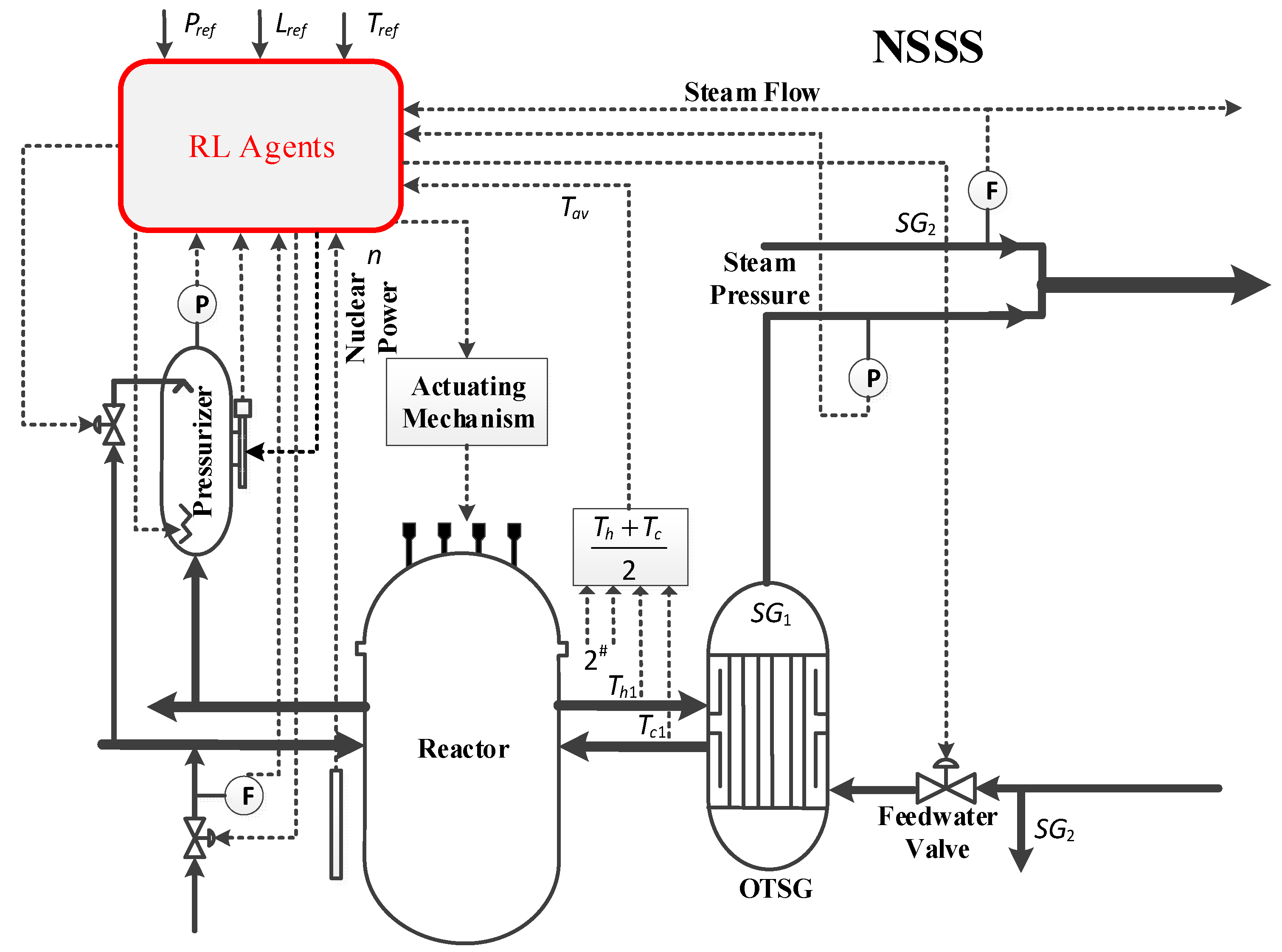
3.1. RL-Based Reactor Control System Structure and Principles

There exists a strong coupling between the controlled variables in an SPWR system, and the traditional control methods do not take such coupling into account, making it difficult to achieve superior control effects. Instead of the traditional PID control system, the agent in RL is used, i.e., each independent decentralized PID control system in the SPWR is replaced by an agent (shown in Figure 2) in order to optimally regulate the strongly coupled multiple control quantities.

The basic framework of RL mainly includes the environment and the agent, which include the policy network, the value network, the amount of observation of the environment, the amount of action given to the environment, and the rewards that the environment feeds back to the agents, and the environment comprises the NSSS simulation model developed in this study.

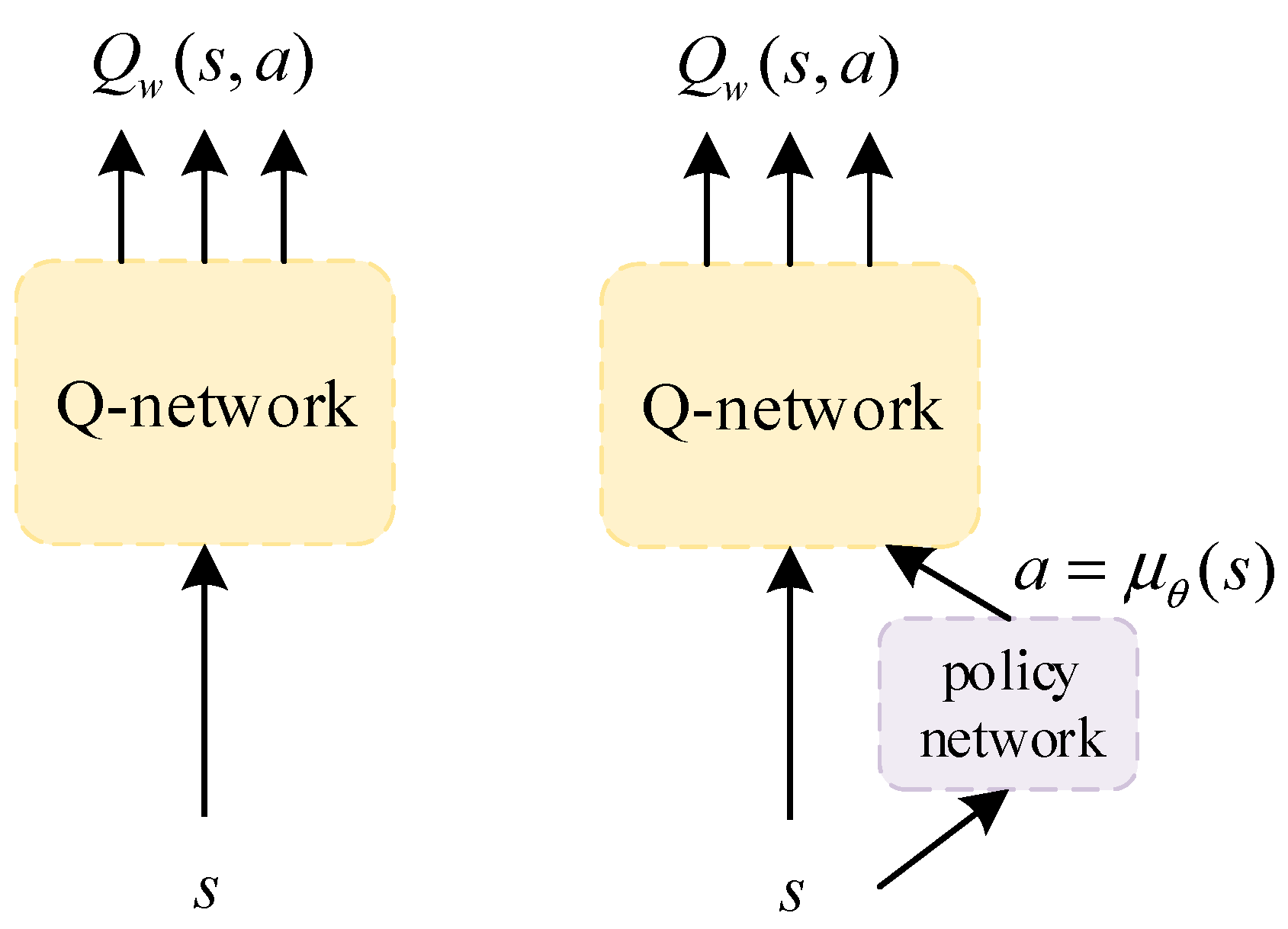
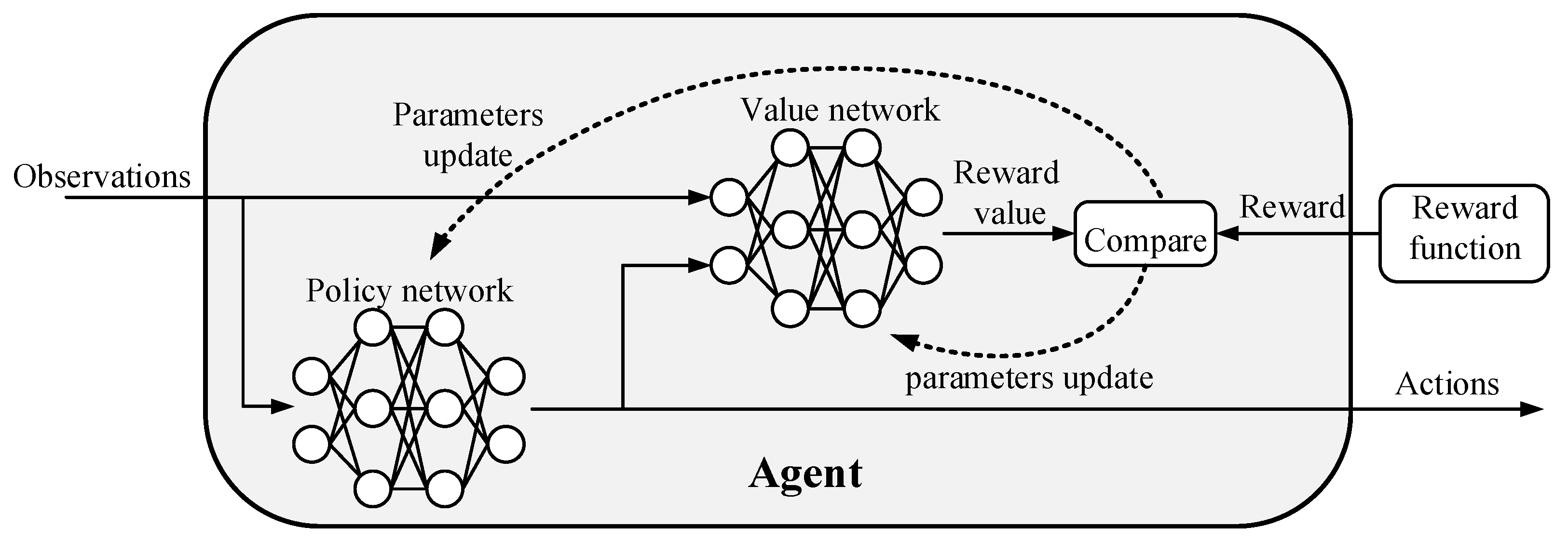
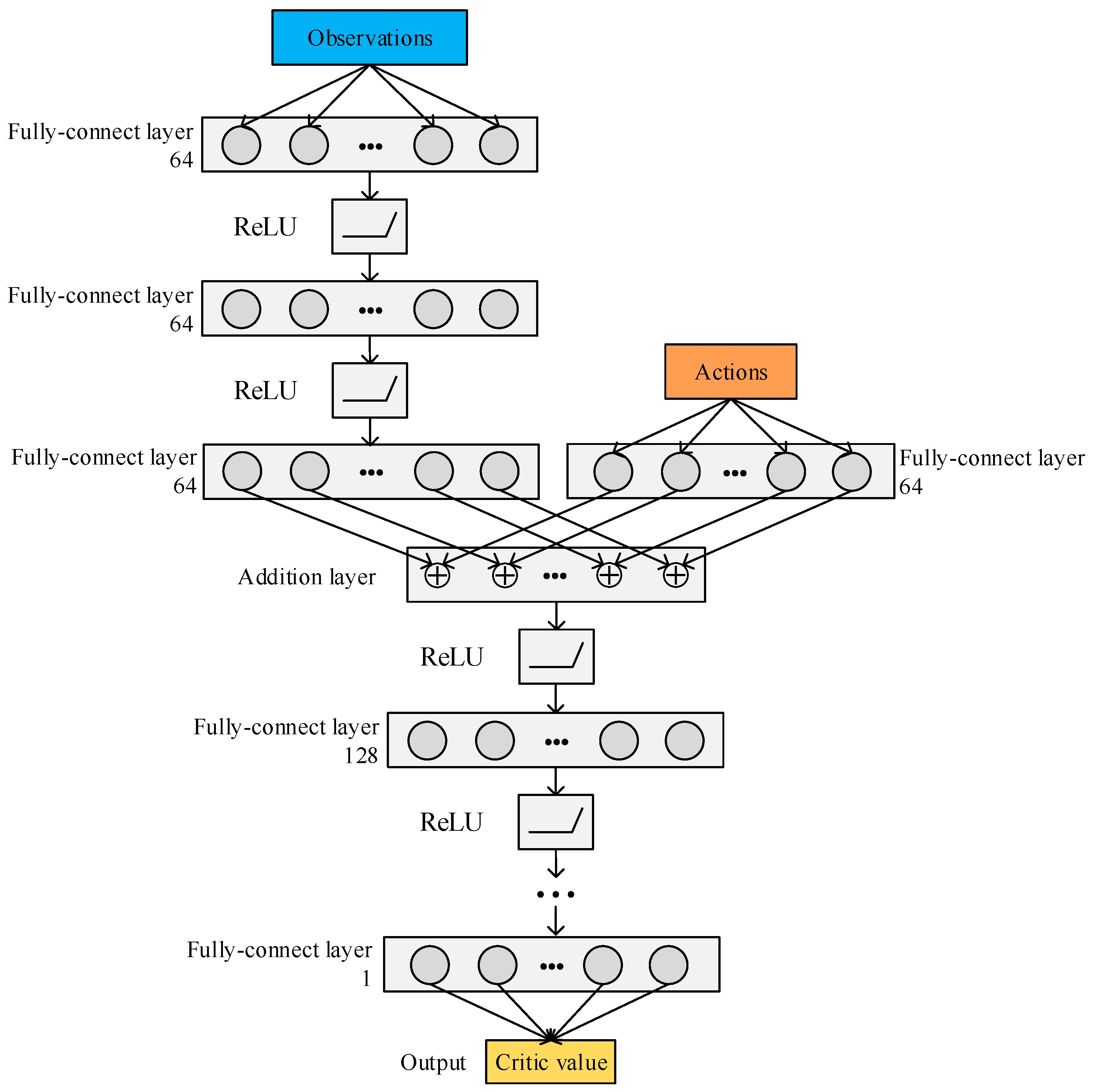
3.2. DDPG Reinforcement Learning Algorithm

DDPG is an extended version of deep Q networks that can be extended to continuous action space [30]. In the training of DDPG, the techniques of deep Q networks are borrowed: target network and experience playback. As a result, the experience playback is consistent with the deep Q network, but the update mechanism for the target network differs from that of the deep Q network. The DDPG is proposed so that the deep Q network can be extended to continuous action spaces, such as cart speed, angle, and voltage, and other similar continuous values. The DDPG adds a policy network on top of the deep Q network to output the action values directly, so the DDPG needs to learn the policy network while learning the Q network, which is illustrated in Figure 3. The Q network’s parameters are represented by $\omega$, while those of the policy network are indicated by $\theta$.

The target network used by DDPG is consistent with the deep $Q$ network algorithm, so in addition to the policy network that needs to be optimized, there is also a network that needs to be optimized as well. The critic does not know how to score initially but slowly gives accurate scores in a step-by-step learning process. In fact, the method of optimizing the $Q$ network is the same as that of optimizing the network for deep $Q$ networks, using the real rewards $r$ and subsequent step $Q$, i.e., $Q^{\prime }$, fitting the future rewards $Q-target$. Subsequently, the $Q$ network’s output is adjusted to closely align with $Q-target$. So, the loss function constructed is a straightforward way to find the mean square deviation of these two values. After constructing the loss function, it is put into the optimizer and minimizes the loss automatically.

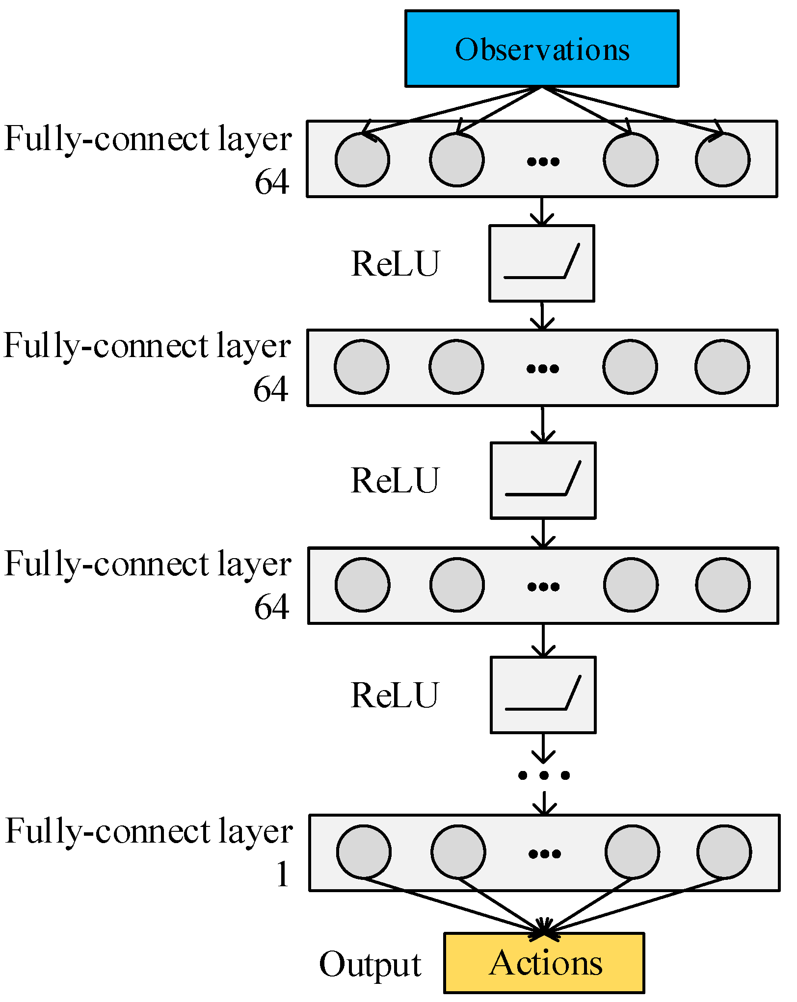
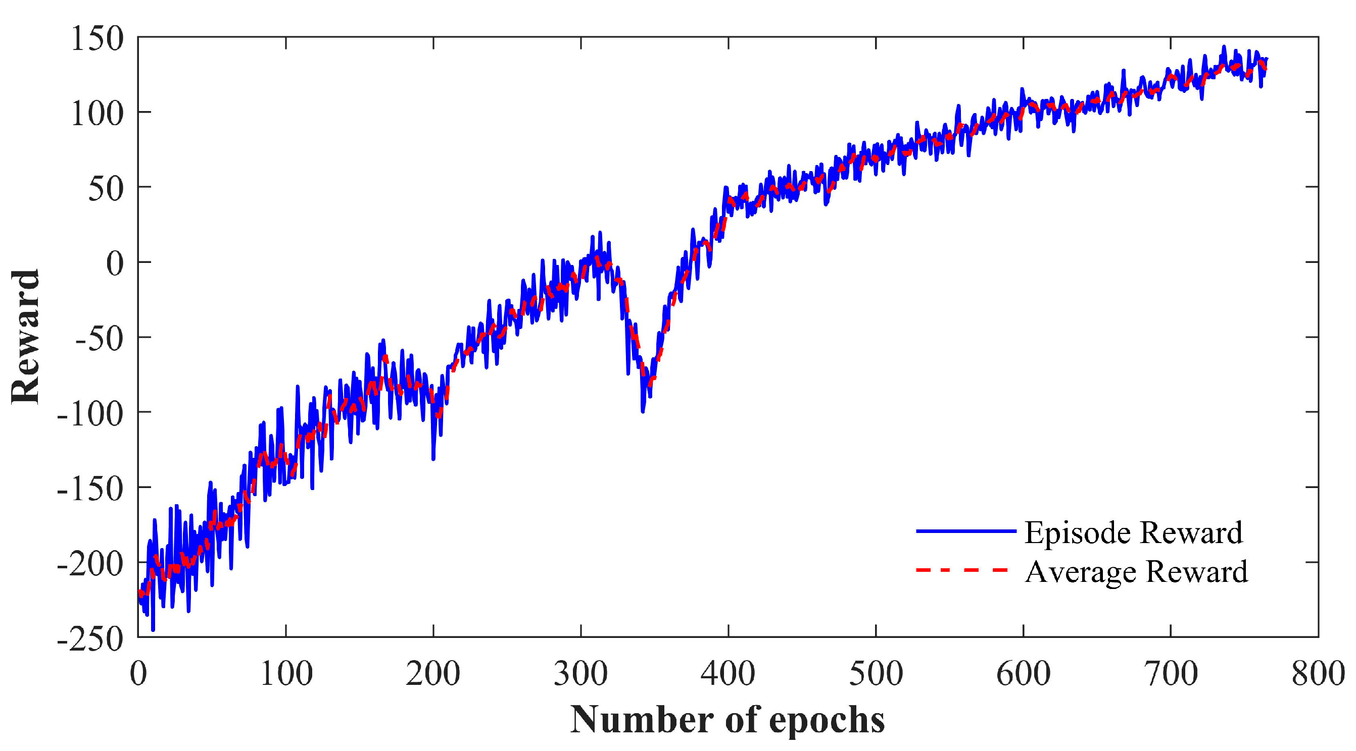
3.3. RL Agents’ Design and Training

Figure 4 illustrates the basic architecture of the DDPG reinforcement learning algorithm employed in this study. The agent comprises two key networks: the policy network and the value network. The policy network gives the corresponding action value according to the current observation value, and the value network gives the corresponding evaluation value according to the observations and actions. Subsequently, the evaluation value is compared with the reward value given by the reward function, and the parameters of strategy and value networks are updated based on the comparison results.

Figure 5 and Figure 6 depict the schematic structures of the strategy and value networks, respectively, primarily consisting of the fully connected layer and the rule layer. The feature layer serves as the input layer for the strategy network, with the state quantity being the input, i.e., the observation quantity selected in this study. The fully connected layer serves as the output layer, with the action quantity being the output, i.e., the control quantity that the agent outputs to the model. The strategy network has eight fully connect layers, and except for the last fully connected layer, the rest of the fully connected layers include 64 neurons per layer. The value network is a multi-input neural network with two feature input layers, state quantity and action quantity, and the output layer is a fully connected layer. There are four fully connected layers containing 64 neurons each before the addition layer and four fully connect layers containing 128 neurons each after the addition layer except the output layer. It needs to be mentioned that the choice of neural network architectures lacks a universal standard, encompassing aspects such as layer count, neuron quantity, and the selection of nonlinear units. In this study, the initial configuration of layers and neurons was derived from analogous cases in related domains, with subsequent refinements made based on training outcomes. The BP neural network, a widely used structure, is capable of modeling nonlinear systems. Additionally, to maintain practicality, the action network’s design and parameters were kept relatively simple. Given that this study focuses on a complex, time-delayed, and highly nonlinear model, the value network was designed with greater intricacy to precisely assess system states and evaluate the policy network’s performance.

The control simulation model of the SPWR system designed based on the RL framework in MATLAB/Simulink is shown in Figure 7, with the RL agents on the left side and the simulation model of the SPWR system on the right side, and the two are interactively computed through the observation amount of the action amount and so on.

Agent training is conducted in two distinct stages: offline training and online optimization. During the offline training stage, after adjusting the agent value network, the strategy network, and the hyperparameters, RL is used to obtain new network parameters for online optimization in the second phase. In the second phase, the agents used in the training are consistent with the first phase, and after the maximum reward value is obtained, the optimization training is stopped and the neural network parameters in the agents are saved. At this point, all the training steps of the agent are completed.

The observations and actions for offline training and online optimization are consistent as shown in

Table 1. Observations and actions for offline and online training.

	Observed Variables and Control Variables
Observations	Reactor Power/%
	Deviation of Reactor Power from Initial Power/%
	Deviation of Reactor Power from Setpoint Power/%
	Deviation of Average Coolant Temperature/°C
	Deviation of Steam Pressure/MPa
	Deviation of Pressurizer Pressure/MPa
	Deviation of Pressurizer Relative Water Level/%
Actions	Control Rod Position/step
	Feedwater Valve Opening/%
	Electric Heater Power/kW
	Spray Valve Opening/%
	Charging Valve Opening/%

.

The reward function is structured as

$$R=R_e+R_a+R_l+R_t$$

(12)

where $R_e$ is the main penalty factor, given according to the deviation; $R_a$ is the secondary penalty factor, given according to the change in the amount of action; $R_l$ is the main incentive factor, given according to the degree of proximity to the target value; and $R_t$ is the absolute penalty factor, given according to the running time.

$$R_e=-10{(T_{avg\_ref}-T_{avg})}^2-10{(P_{h\_ref}-P_h)}^2-10{(P_{zr\_ref}-P_{zr})}^2-10{(P_{zrL\_ref}-P_{zrL})}^2$$

(13)

$$R_a=-{V_{rod}}^2-0.04{(C_{fv\_ref}-C_{fv})}^2-0.02{(Q_{h0}-Q_h)}^2-0.04{C_{sp}}^2-0.04{C_{cv}}^2$$

(14)

$$R_l=10R_{l\_T}+10R_{l\_Ph}+10R_{l\_Pzr}+10R_{l\_PzrL}$$

(15)

$$R_t=-230\times isdone\times {\displaystyle \frac{T_f-t}{T_s}}$$

(16)

where $T_{avg\_ref}$ represents the coolant average temperature set value; $T_{avg}$ indicates the coolant average temperature in actual operation; $P_{h\_ref}$ is the set value of steam pressure; $P_h$ denotes the steam pressure in actual operation; $P_{zr\_ref}$ is the pressurizer set pressure; $P_{zr}$ is the pressurizer pressure in actual operation; $P_{zrL\_ref}$ is the initial pressurizer relative water level; $P_{zrL}$ is the pressurizer relative water level in actual operation; $V_{rod}$ is the control rod speed; $C_{fv\_ref}$ is the reference feed water valve opening; $C_{fv}$ is the actual feed water valve opening; $Q_{h0}$ is the initial electric heater power; $Q_h$ represents the electric heater power during the actual operation; $C_{sp}$ is the spray valve opening; $C_{cv}$ is the upstroke valve opening; $isdone$ is the program abort signal, which is taken as the value of 0 or 1 when the system state significantly deviates from its normal condition under the effect of the random action quantity, and the round of training is ended in advance when the aborting is performed in advance, $isdone=1$; T_f is the simulation time of each round; T_s represents the time step; t denotes the system running time; and $R_{l\_T}$, $R_{l\_Ph}$, $R_{l\_Pzr}$, and $R_{l\_PzrL}$ are the average coolant temperature, steam pressure, pressurizer pressure, and pressurizer water level close to the target reward, respectively.

$$R_{l\_T}=\left\{\begin{array}{l}-{\displaystyle \frac{1}{0.05}}\times \left|T_{avg\_ref}-T_{avg}\right|+1,\left|T_{avg\_ref}-T_{avg}\right|\le 0.05\\ e^{-\left|T_{avg\_ref}-T_{avg}\right|+0.05}-1,\left|T_{avg\_ref}-T_{avg}\right|>0.05\end{array}\right.$$

(17)

$$R_{l\_Ph}=\left\{\begin{array}{l}-{\displaystyle \frac{1}{0.0005}}\times \left|P_{h\_ref}-P_h\right|+1,\left|P_{h\_ref}-P_h\right|\le 0.0005\\ e^{-\left|P_{h\_ref}-P_h\right|+0.0005}-1,\left|P_{h\_ref}-P_h\right|>0.0005\end{array}\right.$$

(18)

$$R_{l\_Pzr}=\left\{\begin{array}{l}-{\displaystyle \frac{1}{0.0005}}\times \left|P_{zr\_ref}-P_{zr}\right|+1,\left|P_{zr\_ref}-P_{zr}\right|\le 0.0005\\ e^{-\left|P_{zr\_ref}-P_{zr}\right|+0.0005}-1,\left|P_{zr\_ref}-P_{zr}\right|>0.0005\end{array}\right.$$

(19)

$$R_{l\_PzrL}=\left\{\begin{array}{l}-{\displaystyle \frac{1}{0.05}}\times \left|P_{zrL\_ref}-P_{zrL}\right|+1,\left|P_{zrL\_ref}-P_{zrL}\right|\le 0.05\\ e^{-\left|P_{zrL\_ref}-P_{zrL}\right|+0.05}-1,\left|P_{zrL\_ref}-P_{zrL}\right|>0.05\end{array}\right.$$

(20)

Figure 8 and Figure 9 depict the offline and online training processes, respectively. The offline training dataset comprises observations and control actions derived from a conventional PID control system across various typical transient scenarios. From this dataset, 70% was randomly allocated as the training set, with the remaining 30% serving as the validation set. Offline training is relatively time efficient, with each session lasting around 2 h. In contrast, online training requires approximately 693 h. As the number of training rounds increases, the reward for the agent increases.

4. Simulations and Analyses

The mentioned advanced control methods in Section 1 are mainly aimed at improving the control performance in a single system or coupling control of limited parameters, while the proposed RL-based strategies can solve the coupling control of more variables in the reactor control system, including the reactor power, average coolant temperature, steam pressure, pressure of the pressurizer, and relative liquid level. Given that the conventional PID control system is currently the most widely used reactor control method, this paper adopts PID as the benchmark for simulation comparison. The performance of the RL agents established for the SPWR in this paper is verified by evaluating the control effect against that of the conventional PID control system under several typical load change transients.

4.1. The ±10% FP Step Load Change Transients

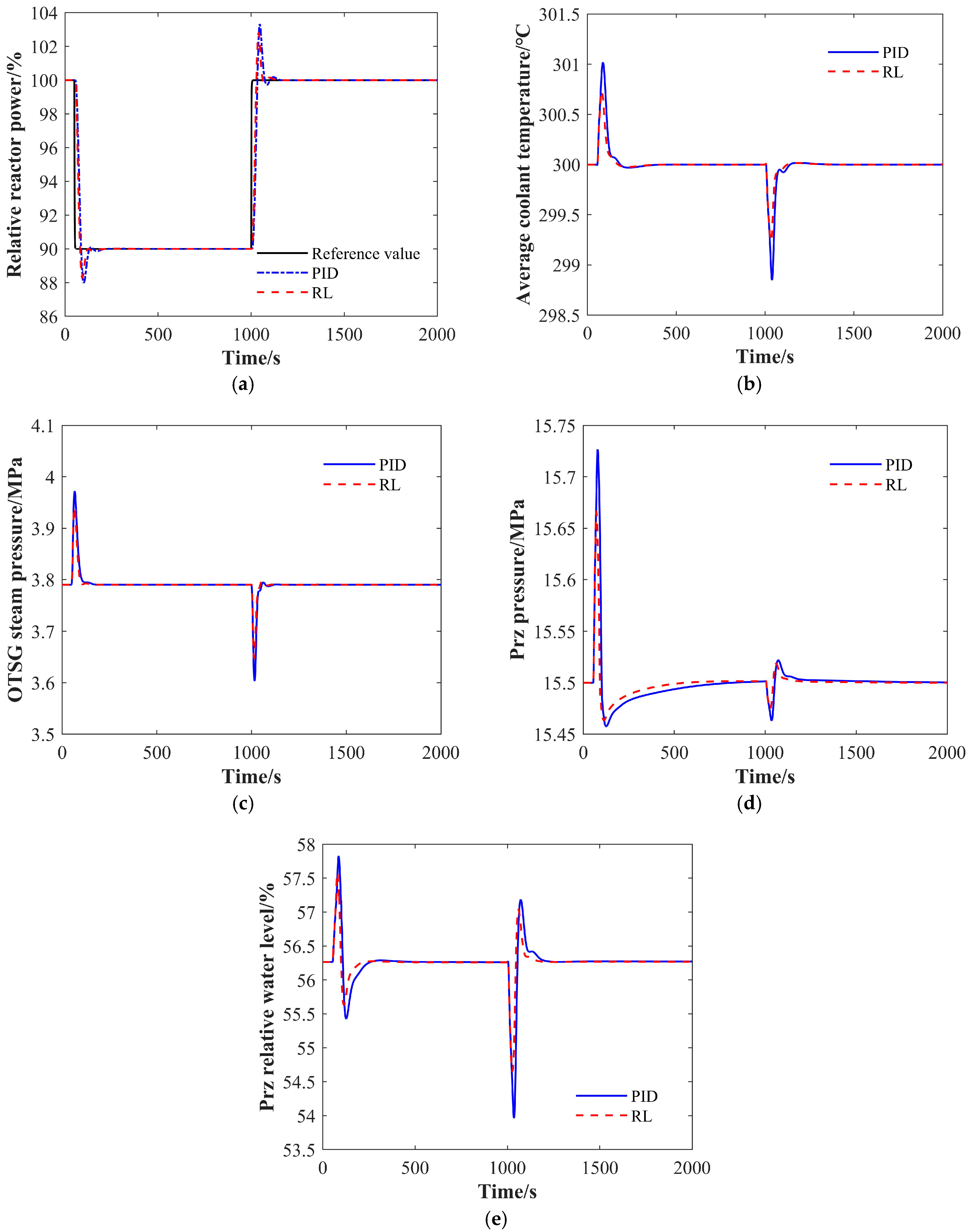
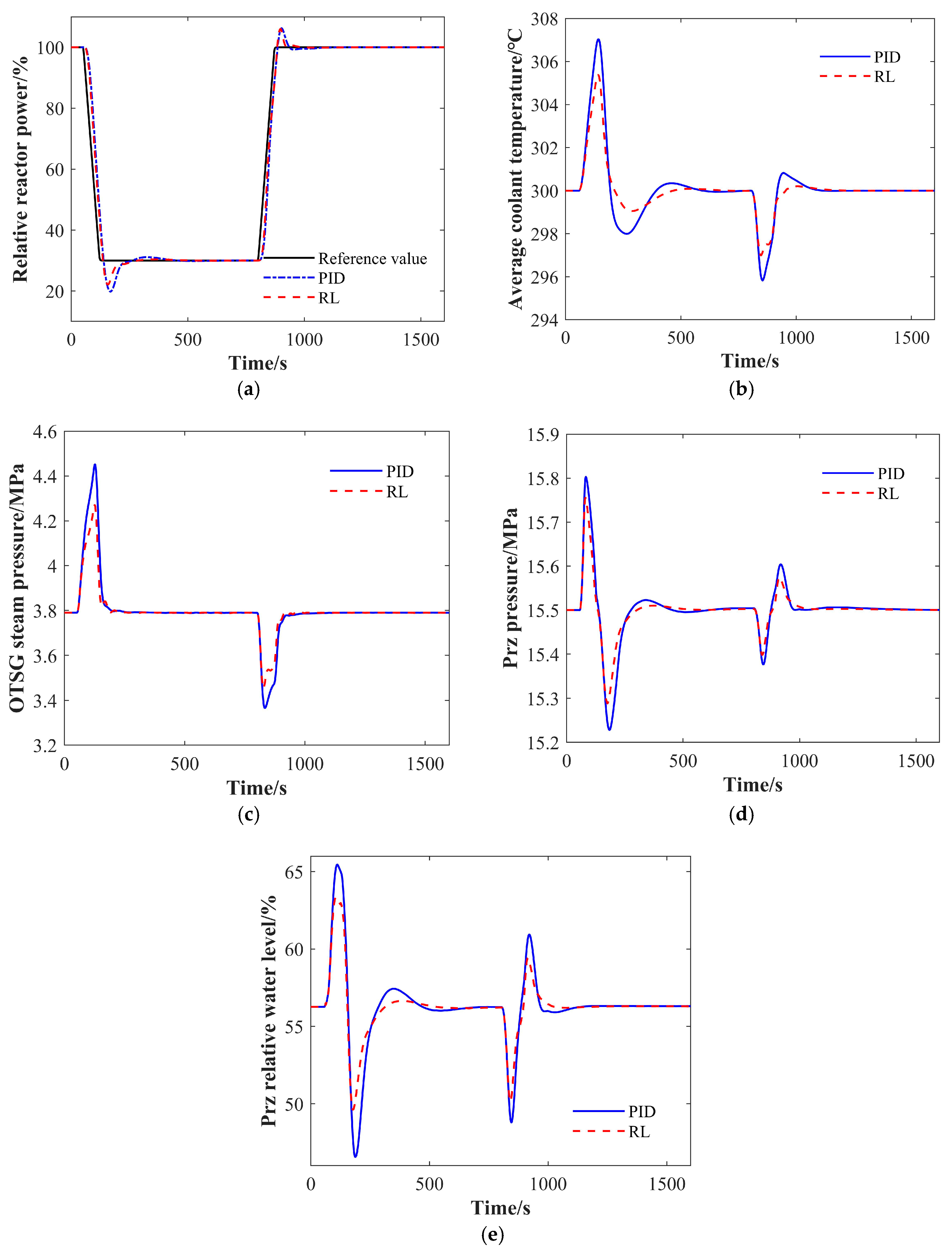
4.1.1. The 100% FP-90% FP-100% FP Condition

The SPWR simulation model is operated stably at a 100% FP power level. At t = 50 s, the load changes step to 90% FP, and at t = 1000 s, the load changes step to 100% FP. Figure 10 illustrates the transient behaviors of key parameters, including the normalized reactor power, mean coolant temperature, OTSG steam pressure, pressurizer pressure, and normalized water level. The legend identifies three curves: the “Reference value” denotes the load setpoint trajectory, “PID” corresponds to conventional PID controller performance, and “RL” reflects the outcomes of reinforcement-learning-based control.

The simulation results, shown in Figure 10, demonstrate that reactor power is effectively tracked using either PID or RL control. Furthermore, the average coolant temperature, steam pressure, pressurizer pressure, and water level remain stable after a brief transient. The pressurizer pressure control system adjusts the pressure by regulating the electric heater power and spray flow rate. The rate of pressure increase through electric heater heating exceeds the rate of pressure decrease via spraying, resulting in minimal pressure deviation during the transition from 90% FP to 100% FP.

In comparison to the conventional PID control system, the RL agent exhibits smaller power overshoot, a shorter regulation time, and lower maximum deviation peaks for average coolant temperature, steam pressure, pressurizer pressure, and water level. Additionally, its regulation time is better than or basically equivalent to that of the conventional PID system. That is, the RL-based control outperforms the traditional PID approach.

The significant overshoot or deviation of physical and thermal parameters such as the reactor power and average coolant temperature during transient processes can deteriorate equipment operating conditions in a nuclear power plant. In extreme cases, this may shorten equipment lifespan and compromise plant safety. Therefore, minimizing overshoot and deviation during transients is crucial for improving nuclear power plant safety. To facilitate a more direct comparison of the performance between RL-based and PID control systems, quantitative indicators were computed under the given conditions, as presented in

Table 2. Performance metrics of RL and PID under 100% FP-90% FP-100% FP condition.

	Power		Tavg		Ph		Prz		PrzL
	σ/%	ts/s	∆/°C	ts/s	∆/MPa	ts/s	∆/MPa	ts/s	∆/%	ts/s
PID	3.32	71	1.15	116	0.19	47	0.23	312	2.30	159
RL	2.80	60	0.76	93	0.14	37	0.17	202	1.60	112
Optimization Improvement/%	15.8	15.5	33.9	19.0	23.8	21.3	26.8	35.3	30.2	29.6

. The table shows that σ, ∆, and t_s correspond to overshoot, maximum deviation, and settling time, respectively. Apparently, the RL-based control system outperforms the traditional PID control system in terms of overshoot, maximum deviation, and settling time.

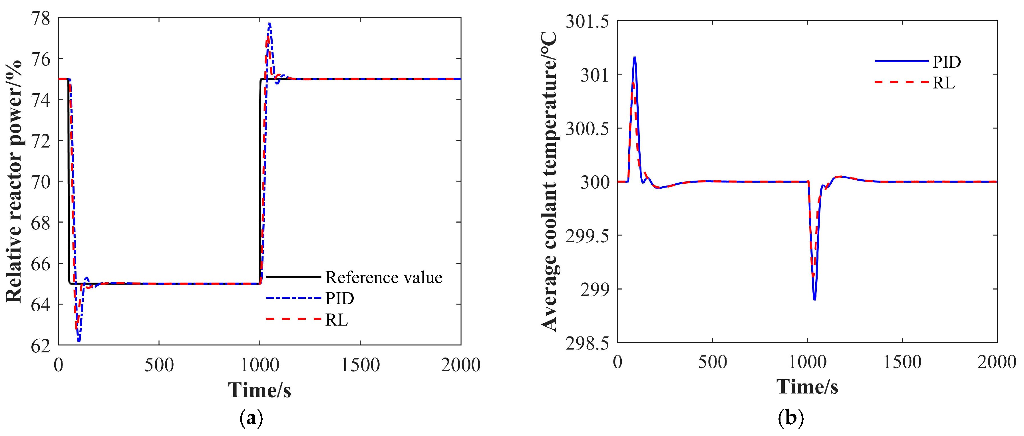
4.1.2. The 75% FP-65% FP-75% FP Condition

The SPWR simulation model is operated stably at a 75% FP power level. At t = 50 s, the load changes step to 65% FP, and at t = 1000 s, the load changes step to 75% FP. The dynamic responses of the reactor relative power, average coolant temperature, OTSG steam pressure, pressurizer pressure, and relative water level are presented in Figure 11. A comparison of the control performance indicators is provided in

Table 3. Performance metrics of RL and PID under 75% FP-65% FP-75% FP condition.

	Power		Tavg		Ph		Prz		PrzL
	σ/%	ts/s	∆/°C	ts/s	∆/MPa	ts/s	∆/MPa	ts/s	∆/%	ts/s
PID	4.44	73	1.16	175	0.26	42	0.23	329	2.24	161
RL	3.48	59	0.92	50	0.18	35	0.18	209	1.87	110
Optimization Improvement/%	21.6	19.2	20.9	71.4	30.2	16.7	23.4	36.5	16.5	31.7

.

It can be seen from Figure 11 that the reactor system is able to realize the control of the established goals under the control effect of either PID or RL. Compared with the traditional PID control system, the power overshoot and regulation time under the control of RL are smaller, the average coolant temperature, steam pressure, pressurizer pressure and relative water level deviation peaks are lower, and the regulation time is shorter, which indicates that the control effect of RL obtained by design and training is better than that of the traditional PID control system.

As shown in Figure 11 and Table 3, the reactor system achieves the established control goals under both PID and RL control. Compared to the conventional PID control system, RL control results in smaller power overshoot, a shorter regulation time, and lower deviation peaks for the average coolant temperature, steam pressure, pressurizer pressure, and relative water level. These improvements demonstrate that the RL control, designed and trained, outperforms the conventional PID.

4.1.3. The 50% FP-40% FP-50% FP Condition

The SPWR simulation model is operated stably at a 50% FP power level. At t = 50 s, the load changes step to 40% FP, and at t = 1000 s, the load changes step to 50% FP. The dynamic responses of the reactor relative power, average coolant temperature, OTSG steam pressure, pressurizer pressure, and relative water level are presented in Figure 12. A comparison of control performance indicators is provided in

Table 4. Performance metrics of RL and PID under 50% FP-40% FP-50% FP condition.

	Power		Tavg		Ph		Prz		PrzL
	σ/%	ts/s	∆/°C	ts/s	∆/MPa	ts/s	∆/MPa	ts/s	∆/%	ts/s
PID	10.7	100	1.66	203	0.35	63	0.26	344	3.33	160
RL	8.53	63	1.24	95	0.24	37	0.20	229	2.78	125
Optimization Improvement/%	20.6	37.0	25.5	53.2	31.6	41.3	25.1	33.4	16.5	21.9

.

As shown in Figure 12 and Table 4, the reactor system operates stably and normally under both PID and RL control. Compared to the conventional PID control system, the RL control results in smaller power overshoot, a shorter regulation time, and lower maximum deviation peaks for the average coolant temperature, steam pressure, pressurizer pressure, and relative water level.

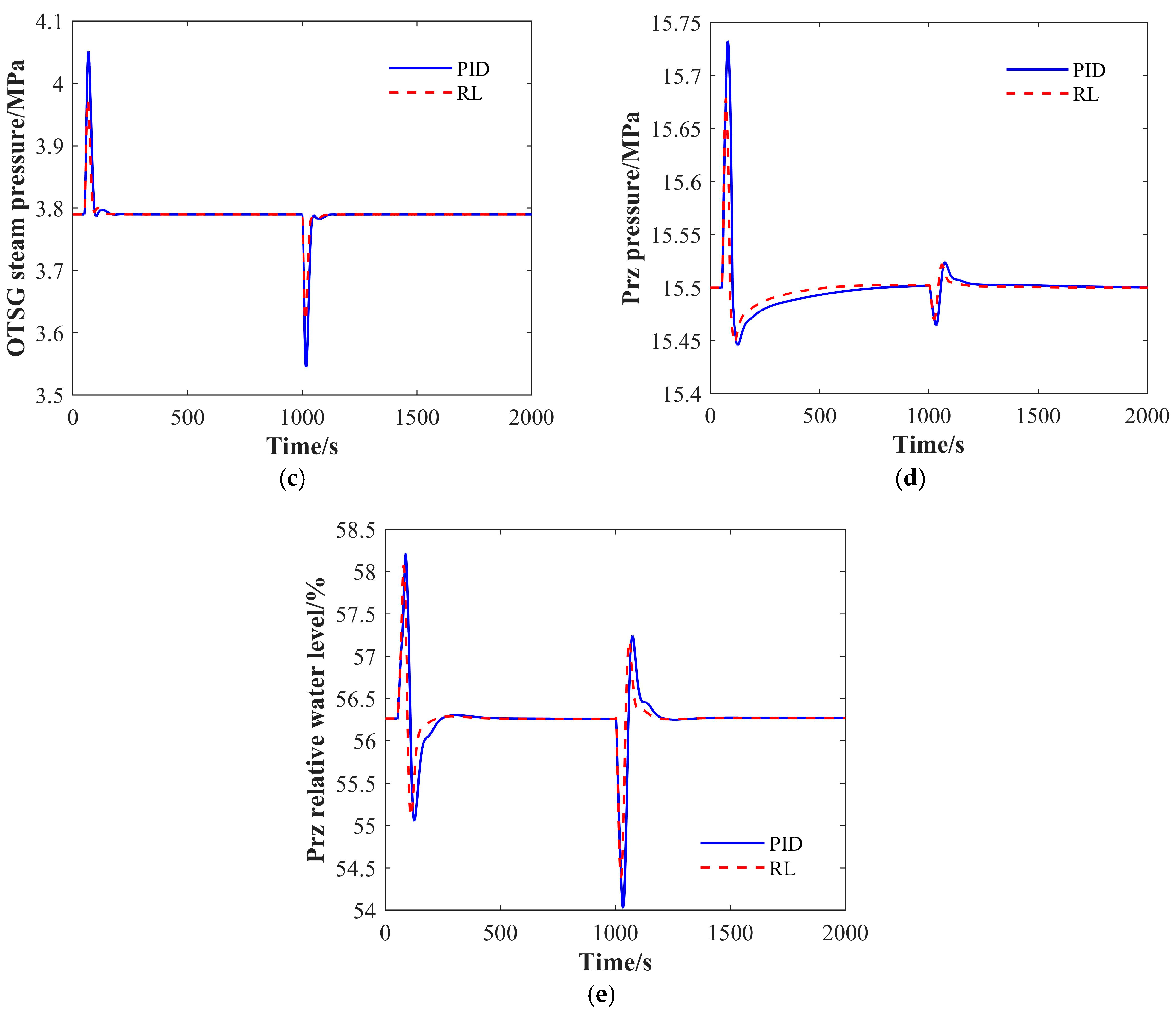
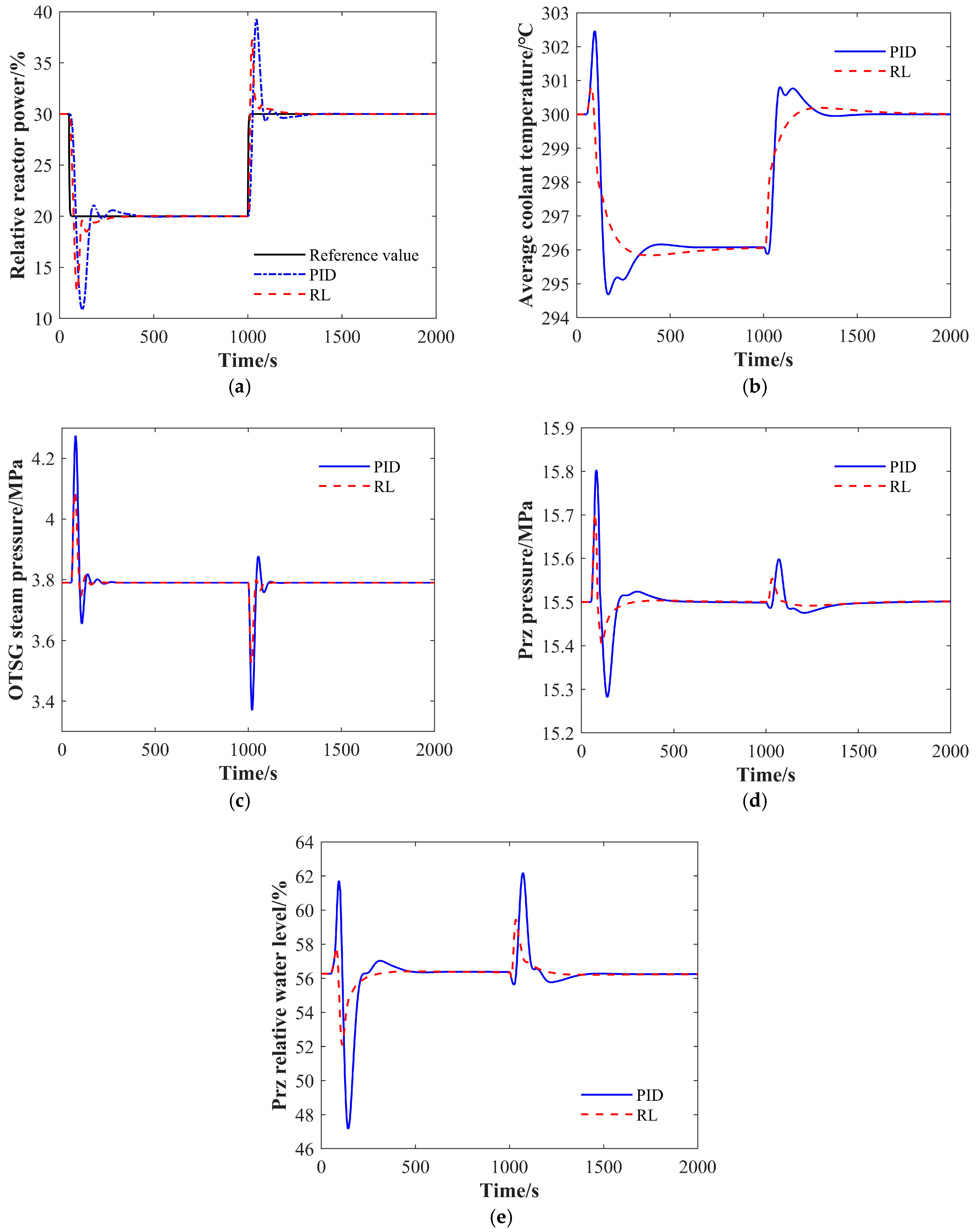
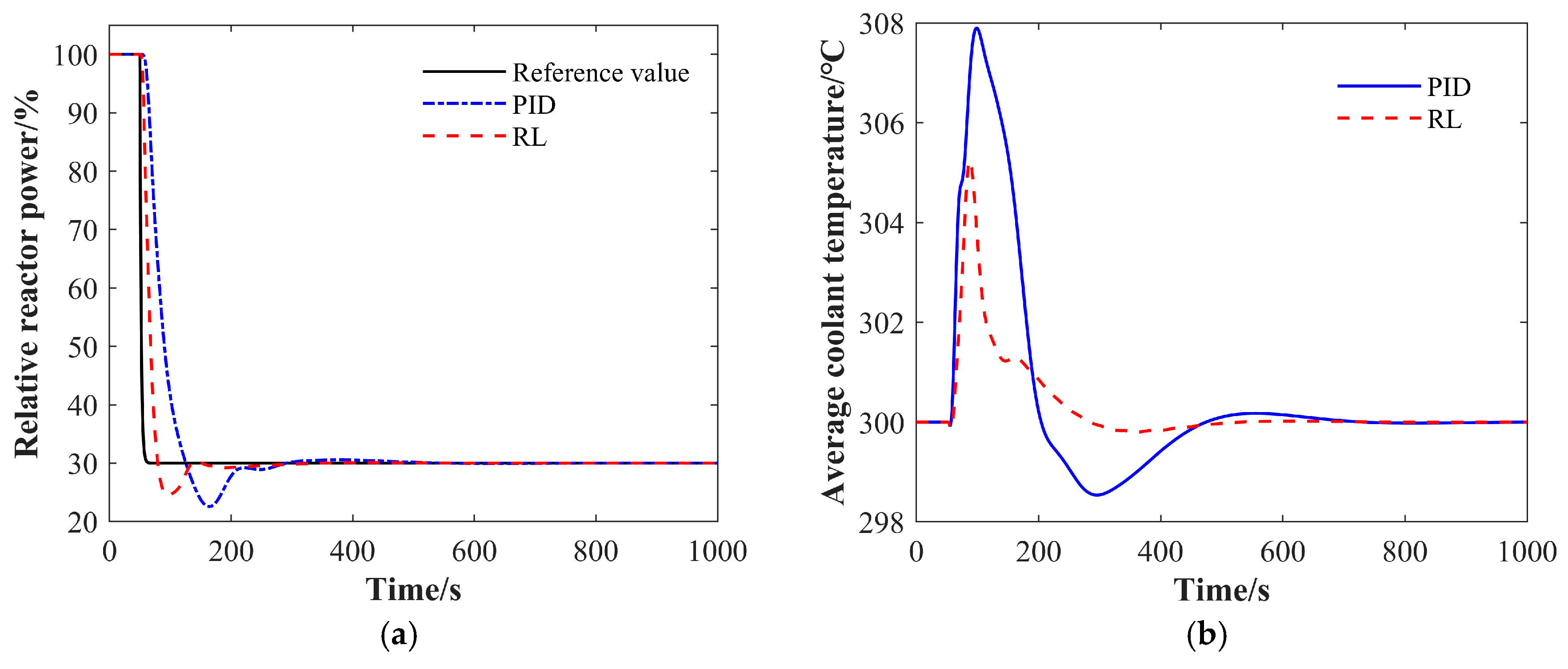
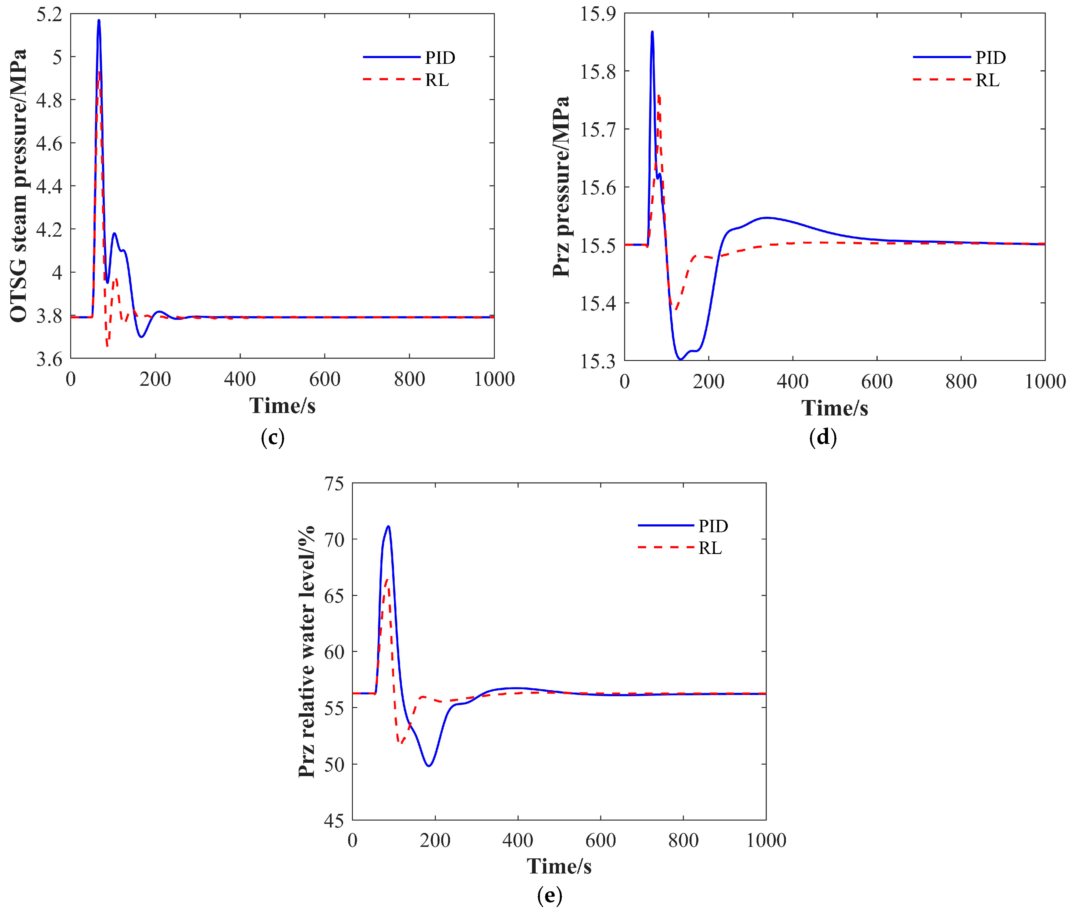
4.1.4. The 30% FP-20% FP-30% FP Condition

The SPWR simulation model operates stably at a 30% FP power level. At t = 50 s, the load changes step to 20% FP, and at t = 1000 s, the load changes step to 30% FP. The dynamic responses of the reactor relative power, average coolant temperature, OTSG steam pressure, pressurizer pressure, and relative water level are presented in Figure 13. A comparison of control performance indicators is provided in

Table 5. Performance metrics of RL and PID under 30% FP-20% FP-30% FP condition.

	Power		Tavg		Ph		Prz		PrzL
	σ/%	ts/s	∆/°C	ts/s	∆/MPa	ts/s	∆/MPa	ts/s	∆/%	ts/s
PID	45.9	253	2.47	279	0.48	92	0.30	312	9.10	331
RL	36.6	156	0.81	163	0.30	67	0.20	138	4.17	155
Optimization Improvement/%	20.2	38.3	67.2	41.6	38.3	27.2	33.2	55.8	54.2	53.2

.

We can see from Figure 13 and Table 5 that when the core power step-down to 20% FP occurs, the coolant average temperature is no longer stabilized at 300 °C but is in a new steady state according to the one-loop coolant average temperature operation scheme. Compared with the simulation results at high and medium power levels, the overshooting amount of the core power, the coolant average temperature, and the steam pressure deviation are larger, which is consistent with the results of the operational characterization. The simulation results show that both PID and RL control effectively track reactor power, while maintaining constant coolant average temperature and steam pressure. The control performance indexes under RL-based control are significantly better than those of the conventional PID control system. The comparison results in Table 5 support this analysis.

4.2. Ramp Load Change Transients

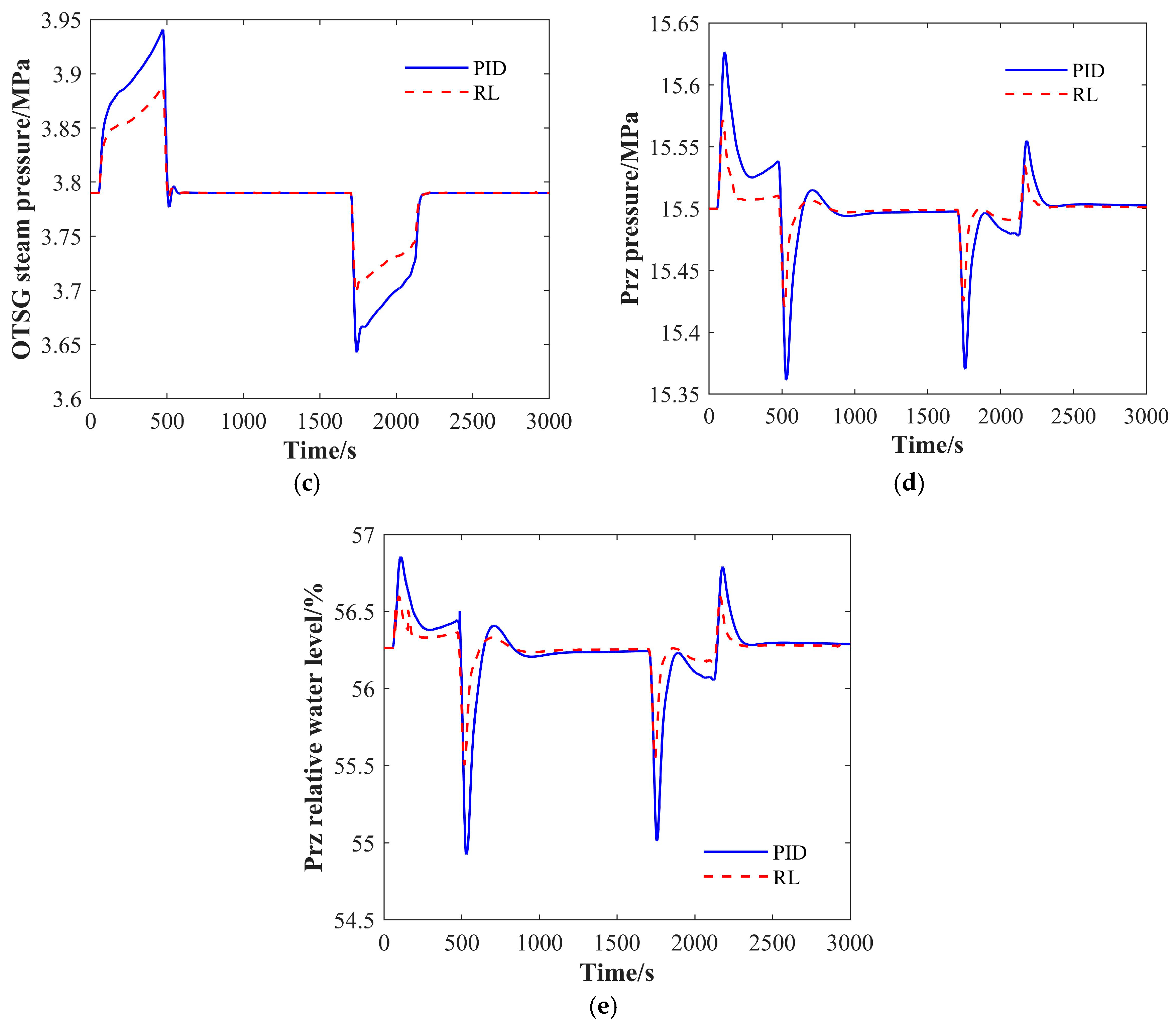
4.2.1. The ±10% FP/min Ramp Load Change Transient

The SPWR simulation model is operated stably at a 100% FP power level. At t = 50 s, the load changes to 30% FP at a rate of −10% FP/min then changes to 100% FP at t = 1700 s at a rate of 10% FP/min. The dynamic responses of the reactor relative power, average coolant temperature, OTSG steam pressure, pressurizer pressure, and relative water level are presented in Figure 14. A comparison of the control performance indicators is provided in

Table 6. Performance metrics of RL and PID under ±10% FP/min ramp load change transient.

	Power		Tavg		Ph		Prz		PrzL
	σ/%	ts/s	∆/°C	ts/s	∆/MPa	ts/s	∆/MPa	ts/s	∆/%	ts/s
PID	7.41	62	0.97	164	0.15	52	0.14	312	1.34	312
RL	5.46	51	0.67	73	0.10	29	0.08	124	0.76	124
Optimization Improvement/%	26.4	17.7	30.6	55.5	34.8	44.2	43.2	60.3	43.4	60.3

.

As shown in Figure 14 and Table 6, under the linear variable-load condition, the load tracking is excellent due to the slower power change, resulting in minimal deviation of average coolant temperature and steam pressure. Compared to the conventional PID control system, RL-based control shows significant improvements in core relative power overshoot, average coolant temperature, steam pressure, pressurizer pressure, and maximum level deviation. Additionally, core relative power, average coolant temperature, steam pressure, pressurizer pressure, and level adjustment times are all better under RL control.

4.2.2. The ±1% FP/s Ramp Load Change Transient

The SPWR simulation model is operated stably at 100% FP power level. At t = 50 s, the load changes to 30% FP at a rate of −1% FP/s, then changes to 100% FP at t = 800 s at a rate of 1% FP/s. The dynamic responses of reactor relative power, average coolant temperature, OTSG steam pressure, pressurizer pressure, and relative water level are presented in Figure 15. A comparison of control performance indicators is provided in

Table 7. Performance metrics of RL and PID under ±1% FP/s ramp load change transient.

	Power		Tavg		Ph		Prz		PrzL
	σ/%	ts/s	∆/°C	ts/s	∆/MPa	ts/s	∆/MPa	ts/s	∆/%	ts/s
PID	33.9	272	7.03	148	0.66	39	0.30	269	9.71	304
RL	26.3	132	5.38	51	0.48	20	0.26	148	6.65	164
Optimization Improvement/%	22.6	51.5	23.5	65.5	27.5	48.7	15.8	45.0	31.5	46.1

.

Figure 15 and Table 7 illustrate that under the linear variable-load condition, despite the faster power change rate, good load tracking is achieved, and the deviations in the average coolant temperature and steam pressure are significantly larger compared to the slower load change condition. Compared with the traditional PID control system, the optimization effect of the core relative power overshoot, average coolant temperature, steam pressure, pressurizer pressure, and liquid level maximum deviation under the control of the enhanced learning agent is remarkable, and the core relative power, average coolant temperature, steam pressure, pressurizer pressure, and liquid level adjustment time are also better than that of the PID control system. Compared with the ±10% FP/min linear variable-load condition, the optimization effect of reinforcement learning control is more significant under the fast variable-load condition.

4.3. Load Rejection Transient

The SPWR simulation model is operated stably at a 100% FP power level. At t = 50 s, the load changes step to 30% FP. The dynamic responses of the reactor relative power, average coolant temperature, OTSG steam pressure, pressurizer pressure, and relative water level are presented in Figure 16. A comparison of the control performance indicators is provided in

Table 8. Performance metrics of RL and PID under load rejection transient.

	Power		Tavg		Ph		Prz		PrzL
	σ/%	ts/s	∆/°C	ts/s	∆/MPa	ts/s	∆/MPa	ts/s	∆/%	ts/s
PID	24.9	222	7.90	369	1.38	126	0.37	452	14.9	233
RL	18.4	178	5.23	187	1.14	65	0.26	183	10.1	165
Optimization Improvement/%	26.0	19.8	33.7	49.3	17.6	48.4	28.2	59.5	32.1	29.2

.

It can be seen from Figure 16 and Table 8 that the average coolant temperature and steam pressure change drastically under the load dump condition, and both the PID and RL agents can realize the reactor load tracking, the double constant control of the average coolant temperature and steam pressure, and the stabilization control of the pressurizer pressure and relative water level. Compared with the traditional PID control system, the reinforced learning agent control effect is better.

5. Conclusions

Aiming at the problems of slow response speed and poor coordination existing in the traditional reactor control system architecture based on independent decentralized control loops, research on multivariate control technology for reactor systems was carried out, and a multivariate control system for a reactor system based on RL was established. The control effect of the designed and trained RL agents was verified through simulation analysis. The simulation results show that the control effect of the RL agents is better than that of the traditional PID control effect, and it can optimize the reactor power overshooting amount and regulation time based on the PID control effect, the average coolant temperature, the steam pressure, the pressure of the voltage pressurizer, and the liquid level in the ±10% FP step variable load condition, the ±10% FP/min and the ±1% FP/s linear variable load condition, and the dumping load condition. It has a maximum deviation and regulation time of 15%. This study verifies the effectiveness and advancement of RL agent control for the NSSS of an SPWR.

References

1. Zhou, G.; Tan, D. Review of nuclear power plant control research: Neural network-based methods. Ann. Nuclear Energy 2023, 181, 109513. [Google Scholar] [CrossRef]
2. Podlubny, I. Fractional-order systems and fractional-order controllers. Inst. Exp. Phys. Slovak. Acad. Sci. Kosice 1994, 12, 1–18. [Google Scholar]
3. Gupta, D.; Goyal, V.; Kumar, J. Design of fractional-order NPID controller for the NPK model of advanced nuclear reactor. Prog. Nucl. Energy 2022, 150, 104319. [Google Scholar] [CrossRef]
4. Zeng, W.; Jiang, Q.; Liu, Y.; Yan, S.; Zhang, G.; Yu, T.; Xie, J. Core power control of a space nuclear reactor based on a nonlinear model and fuzzy-PID controller. Prog. Nucl. Energy 2021, 132, 103564. [Google Scholar] [CrossRef]
5. Torabi, K.; Safarzadeh, O.; Rahimi-Moghaddam, A. Robust Control of the PWR Core Power Using Quantitative Feedback Theory. IEEE Trans. Nucl. Sci. 2011, 58, 258–266. [Google Scholar] [CrossRef]
6. Abdulraheem, K.K.; Korolev, S.A. Robust optimal-integral sliding mode control for a pressurized water nuclear reactor in load following mode of operation. Ann. Nucl. Energy 2021, 158, 108288. [Google Scholar] [CrossRef]
7. Li, G.; Liang, B.; Wang, X.; Li, X.; Xia, B. Application of H-Infinity Output Feedback Control with Analysis of Weight Functions and LMI to Nonlinear Nuclear Reactor Cores; Springer International Publishing: Berlin/Heidelberg, Germany, 2017; pp. 457–468. [Google Scholar]
8. Li, G.; Zhao, F. Flexibility control and simulation with multimodel and LQG/LTR design for PWR core load following operation. Ann. Nucl. Energy 2013, 56, 179–188. [Google Scholar] [CrossRef]
9. Li, G. Modeling and LQG/LTR control for power and axial power difference of load-follow PWR core. Ann. Nucl. Energy 2014, 68, 193–203. [Google Scholar] [CrossRef]
10. Fu, J.; Jin, Z.; Dai, Z.; Su, G.H.; Wang, C.; Tian, W.; Qiu, S. Model predictive control for automatic operation of space nuclear reactors: Design, simulation, and performance evaluation. Ann. Nucl. Energy 2024, 199, 110321. [Google Scholar] [CrossRef]
11. Wang, G.; Wu, J.; Zeng, B.; Xu, Z.; Wu, W.; Ma, X. Design of a model predictive control method for load tracking in nuclear power plants. Prog. Nucl. Energy 2017, 101, 260–269. [Google Scholar] [CrossRef]
12. Naimi, A.; Deng, J.; Vajpayee, V.; Becerra, V.; Shimjith, S.R.; Arul, A.J. Nonlinear Model Predictive Control Using Feedback Linearization for a Pressurized Water Nuclear Power Plant. IEEE Access 2022, 10, 16544–16555. [Google Scholar] [CrossRef]
13. Khansari, M.E.; Sharifian, S. A deep reinforcement learning approach towards distributed Function as a Service (FaaS) based edge application orchestration in cloud-edge continuum. J. Netw. Comput. Appl. 2025, 233, 104042. [Google Scholar] [CrossRef]
14. Wang, J.; Liang, S.; Guo, M.; Wang, H.; Zhang, H. Adaptive multimodal control of trans-media vehicle based on deep reinforcement learning. Eng. Appl. Artif. Intell. 2025, 139, 109524. [Google Scholar] [CrossRef]
15. Gong, A.; Chen, Y.; Zhang, J.; Li, X. Possibilities of reinforcement learning for nuclear power plants: Evidence on current applications and beyond. Nucl. Eng. Technol. 2024, 56, 1959–1974. [Google Scholar] [CrossRef]
16. Dong, Z.; Huang, X.; Dong, Y.; Zhang, Z. Multilayer perception based reinforcement learning supervisory control of energy systems with application to a nuclear steam supply system. Appl. Energy 2020, 259, 114193. [Google Scholar] [CrossRef]
17. Yi, Z.; Luo, Y.; Westover, T.; Katikaneni, S.; Ponkiya, B.; Sah, S.; Khanna, R. Deep reinforcement learning based optimization for a tightly coupled nuclear renewable integrated energy system. Appl. Energy 2022, 328, 120113. [Google Scholar] [CrossRef]
18. Zhang, T.; Dong, Z.; Huang, X. Multi-objective optimization of thermal power and outlet steam temperature for a nuclear steam supply system with deep reinforcement learning. Energy 2024, 286, 129526. [Google Scholar] [CrossRef]
19. Li, J.; Liu, Y.; Qing, X.; Xiao, K.; Zhang, Y.; Yang, P.; Yang, Y.M. The application of Deep Reinforcement Learning in Coordinated Control of Nuclear Reactors. J. Phys. Conf. Ser. 2021, 2113, 012030. [Google Scholar] [CrossRef]
20. Cao, D.H.; Pham, T.N.; Hoang, T.H.; Nguyen, V.H. Preliminary study of thermal hydraulics system for small modular reactor type pressurized water reactor used for floating nuclear power plant. In Proceedings of the Vietnam Conference on Nuclear Science and Technology VINANST-14 Agenda and Abstracts, Nha Trang City, Vietnam, 9–11 August 2023; p. 246. [Google Scholar]
21. Phu, T.V.; Nam, T.H.; Khanh, H.V. Application of Evolutionary Simulated Annealing Method to Design a Small 200 MWt Reactor Core. Nucl. Sci. Technol. 2020, 10, 16–23. [Google Scholar] [CrossRef]
22. Hoang, V.K.; Tran, V.P.; Cao, D.H. Study on fuel design for the long-life core of ACPR50S nuclear reactor. In VINATOM-AR—20; Trang, P.T.T., Ed.; International Atomic Energy Agency (IAEA): Vienna, Austria, 2021; pp. 57–59. [Google Scholar]
23. Wang, X.; Wang, M. Development of Advanced Small Modular Reactors in CHINA. Nucl. Esp. 2017, 380, 34–37. [Google Scholar]
24. China General Nuclear Power Corporation (CGN). Design, Applications and Siting Requirements of CGNACPR50(S); China General Nuclear Power Corporation (CGN): Shenzhen, China, 2017. [Google Scholar]
25. Kerlin, T.W.; Katz, E.M.; Thakkar, J.G.; Strange, J.E. Theoretical and experimental dynamic analysis of the HB Robinson nuclear plant. Nucl. Technol. 1976, 30, 299–316. [Google Scholar] [CrossRef]
26. Nuerlan, A.; Wang, P.; Wan, J.; Zhao, F. Decoupling header steam pressure control strategy in multi-reactor and multi-load nuclear power plant. Prog. Nucl. Energy 2020, 118, 103073. [Google Scholar] [CrossRef]
27. Wang, P.; He, J.; Wei, X.; Zhao, F. Mathematical modeling of a pressurizer in a pressurized water reactor for control design. Appl. Math. Model. 2019, 65, 187–206. [Google Scholar] [CrossRef]
28. Wan, J.; Wang, P.; Wu, S.; Zhao, F. Conventional controller design for the reactor power control system of the advanced small pressurized water reactor. Nucl. Technol. 2017, 198, 26–42. [Google Scholar] [CrossRef]
29. Wang, P.; Jiang, Q.; Zhang, J.; Wan, J.; Wu, S. A fuzzy fault accommodation method for nuclear power plants under actuator stuck faults. Ann. Nucl. Energy 2021, 165, 108674. [Google Scholar] [CrossRef]
30. Tan, H. Reinforcement Learning with Deep Deterministic Policy Gradient. In Proceedings of the 2021 International Conference on Artificial Intelligence, Big Data and Algorithms (CAIBDA), Xi’an, China, 28–30 May 2021; pp. 82–85. [Google Scholar]
Figure 1. Schematic diagram of OTSG model control body division.
Energies 18 01517 g001
Figure 2. Schematic structure of reactor control system based on RL agent.
Energies 18 01517 g002
Figure 3. Schematic of deep Q network to DDPG algorithm.
Energies 18 01517 g003
Figure 4. Structure diagram of the DDPG algorithm.
Energies 18 01517 g004
Figure 5. Schematic diagram of policy network structure.
Energies 18 01517 g005
Figure 6. Schematic diagram of the value network structure.
Energies 18 01517 g006
Figure 7. RL-based simulation model for control of SPWR system.
Energies 18 01517 g007
Figure 8. Offline training process curve: (a) RMSE; (b) loss.
Energies 18 01517 g008
Figure 9. Online training process curve.
Energies 18 01517 g009
Figure 10. Dynamic responses of RL and PID under 100% FP-90% FP-100% FP condition: (a) relative reactor power; (b) average coolant temperature; (c) OTSG steam pressure; (d) pressurizer pressure; (e) pressurizer relative water level.
Energies 18 01517 g010
Figure 11. Dynamic responses of RL and PID under 75% FP-65% FP-75% FP condition: (a) relative reactor power; (b) average coolant temperature; (c) OTSG steam pressure; (d) pressurizer pressure; (e) pressurizer relative water level.
Energies 18 01517 g011aEnergies 18 01517 g011b
Figure 12. Dynamic responses of RL and PID under 50% FP-40% FP-50% FP condition: (a) relative reactor power; (b) average coolant temperature; (c) OTSG steam pressure; (d) pressurizer pressure; (e) pressurizer relative water level.
Energies 18 01517 g012
Figure 13. Dynamic responses of RL and PID under 30% FP-20% FP-30% FP condition: (a) relative reactor power; (b) average coolant temperature; (c) OTSG steam pressure; (d) pressurizer pressure; (e) pressurizer relative water level.
Energies 18 01517 g013
Figure 14. Dynamic responses of RL and PID under ±10% FP/min ramp load change transient. (a) relative reactor power; (b) average coolant temperature; (c) OTSG steam pressure; (d) pressurizer pressure; (e) pressurizer relative water level.
Energies 18 01517 g014aEnergies 18 01517 g014b
Figure 15. Dynamic responses of RL and PID under ±1% FP/s ramp load change transient: (a) relative reactor power; (b) average coolant temperature; (c) OTSG steam pressure; (d) pressurizer pressure; (e) pressurizer relative water level.
Energies 18 01517 g015
Figure 16. Dynamic responses of RL and PID under load rejection transient: (a) relative reactor power; (b) average coolant temperature; (c) OTSG steam pressure; (d) pressurizer pressure; (e) pressurizer relative water level.
Energies 18 01517 g016aEnergies 18 01517 g016b