The Impact of the Urban Heat Island and Future Climate on Urban Building Energy Use in a Midwestern U.S. Neighborhood

Abstract

Typical Meteorological Year (TMY) datasets, widely used in building energy modeling, overlook Urban Heat Island (UHI) effects and future climate trends by relying on long-term data from rural stations such as airports. This study addresses this limitation by integrating Urban Weather Generator (UWG) simulations with CCWorldWeatherGen projections to produce microclimate-adjusted and future weather scenarios. These datasets were then incorporated into an Urban Building Energy Modeling (UBEM) framework using Urban Modeling Interface (UMI) to evaluate energy performance across a low-income residential neighborhood in Des Moines, Iowa. Results show that UHI intensity will rise from an annual average of 0.55 °C under current conditions to 0.60 °C by 2050 and 0.63 °C by 2080, with peak intensities in summer. The UHI elevates cooling Energy Use Intensity (EUI) by 7% today, with projections indicating a sharp increase—91% by 2050 and 154% by 2080. The UHI will further amplify cooling demand by 2.3% and 6.2% in 2050 and 2080, respectively. Conversely, heating EUI will decline by 20.0% by 2050 and 40.1% by 2080, with the UHI slightly reducing heating demand. Insulation mitigates cooling loads but becomes less effective for heating demand over time. These findings highlight the need for climate-adaptive policies, building retrofits, and UHI mitigation to manage future cooling demand.

1. Introduction

The current century has witnessed an unprecedented shift in the distribution of the global population, with urban populations expected to rise from 55% in 2018 to nearly 68% by 2050 [1]. This urban growth contributes significantly to global warming, not only through the reduction in vegetation, which is vital for carbon sequestration, but also through the emission of greenhouse gases and anthropogenic heat [2,3]. While urban density can improve energy efficiency in transportation and infrastructure, it also amplifies heat retention and anthropogenic warming. A major consequence of this urban expansion is the Urban Heat Island (UHI) effect, a phenomenon whereby urban areas experience higher temperatures than their rural counterparts [4,5]. The UHI arises from human activities, urban morphology, and the extensive use of materials like asphalt and concrete that trap heat [6,7,8,9,10].

The atmosphere above urban areas is significantly altered by exchanges at the surface, resulting in distinct radiative, thermal, and aerodynamic properties [11]. These changes lead to the development of the UHI effect, which describes how urban areas experience higher temperatures compared to their rural surroundings. The UHI effect can be classified into different types, primarily subsurface, surface, and atmospheric UHIs [12,13]. The subsurface UHI refers to heat retention in the ground beneath urban areas, although it is less studied. The surface UHI describes temperature differences between urban surfaces (like roads and buildings) and rural areas, with satellite imagery, such as Land Remote-Sensing Satellite (LANDSAT) or Moderate Resolution Imaging Spectroradiometer (MODIS), commonly used to analyze it [14]. The atmospheric UHI consists of two layers: the urban boundary layer (UBL) and the urban canopy layer (UCL). The UBL, extending up to 1–2 km, influences the city’s microclimate, with its thickness affected by factors like urban surface albedo and waste heat emissions [13]. Below the boundary level lies the UCL (from ground level to building tops) which is shaped by microclimatic interactions like shading, vegetation, and reduced airflow, with urban design significantly influencing this zone. The UHI in the canopy layer affects both indoor and outdoor temperatures, with greater intensity in city centers, especially during calm, windless nights when cooling is slower. Conversely, an Urban Cool Island (UCI) can form in the morning, as cities warm more slowly than natural landscapes [15,16,17].

The UHI effect has widespread environmental and social consequences and has been observed in cities of all sizes and locations, including London, UK [18]; Dublin, Ireland [19]; Rome, Italy [20]; Mexico City, Mexico [21]; New York and New Jersey, U.S. [22]; Chicago [23], Illinois, U.S.; Tehran [24], Iran; Beijing-Tianjin [25], China; Tokyo [26], Japan; and various urban centers in South Africa [27]. The phenomenon contributes to higher outdoor temperatures, which negatively impact thermal comfort, degrade air quality, and increase the risk of heat-related illnesses, especially in densely populated urban areas [28,29,30,31,32]. The reciprocal relationship between the UHI and building energy consumption is also significant. Elevated urban temperatures can lead to an increase in cooling loads by 10% to 120% during hot seasons and a reduction in heating loads by 3% to 45% during colder months [33]. However, the overall impact on building energy use is highly dependent on a combination of factors, including regional and local climate conditions, as well as architectural and urban characteristics of the built environment.

Addressing current UHI effects is essential for designing both major renovations and new construction, but it is equally important to account for the impacts of climate change and future weather conditions. According to the IPCC’s Sixth Assessment Report [34], global temperatures are projected to rise by 1.5 °C to 2 °C above pre-industrial levels in the coming decades, depending on the emission scenario followed. The Fourth US National Climate Assessment [35] projects a significant increase in extreme heat events, posing substantial risks to human health. Arul Babu et al. [36] highlight the significant energy implications of such changes, reporting that rising temperatures in major Indian cities could lead to a 179% rise in residential cooling energy demand by the 2090s, while heating demand could decrease by up to 100% in certain areas.

This study examines how both UHI and future climate scenarios affect building energy consumption in a low-income neighborhood in Des Moines, Iowa, U.S., which is located in the Cold-Humid (5A) climate zone. Des Moines serves as a representative mid-sized U.S. city, similar to many urban centers with populations of 500,000+, where UHI effects disproportionately impact low-income communities. The city’s hot, humid summers and cold winters, coupled with an increasing frequency of extreme heat events, make it an ideal case study for assessing the energy burden posed by climate change. Additionally, many older homes in historically disinvested neighborhoods lack air conditioning, exacerbating heat exposure risks. However, widely used energy modeling frameworks often rely on rural-based meteorological data, overlooking localized UHI effects and future climate shifts. To address this gap, this study integrates UHI simulations, Urban Weather Generator (UWG) modeling, and future climate projections with Urban Building Energy Modeling (UBEM). By incorporating high-resolution urban morphology and vegetation data—including assessor records for 272 buildings and 1142 trees—this research enhances energy demand projections and informs climate-adaptive urban planning and energy efficiency strategies.

2. Literature Review

2.1. Methods for Measuring and Modeling UHI Effects

The common practice to assess a city’s heat island effect has been to compare air temperatures at naively described ‘urban’ and ‘rural’ sites using either fixed/stationary sites or mobile temperature surveys. Stationary measurements involve the use of fixed weather stations strategically placed at a height of 2–5 m above the ground within urban and rural environments to continuously monitor temperature differences over time. This height places the measurement within the UCL, where the UHI effect is most pronounced due to the interactions between buildings, streets, and human activities. In contrast, mobile surveys use temperature sensors mounted on vehicles or other mobile devices to collect data across different urban zones, providing a more comprehensive spatial understanding of UHI intensity [37].

While measuring the UHI through direct observation is significant for understanding urban climate, it often requires extensive time and resources, making continuous monitoring impractical for large-scale urban studies. To address this, various process-based models have been developed to simulate the canopy-level UHI. These models vary in physical complexity, computational cost, and spatial resolution, with each approach offering distinct advantages and limitations depending on the study’s objectives. Some models operate as standalone urban climate models, such as the Surface Urban Energy and Water Balance Scheme (SUEWS) [38], while others function as nested tools within larger-scale models, such as the Single-Layer Urban Canopy Model (SLUCM) [39], which is linked to the Weather Research and Forecasting model (WRF) [40]. While the SLUCM enhances urban climate representation within mesoscale models by parameterizing urban surface interactions, it simplifies vertical temperature gradients and neglects detailed intra-urban variability, limiting its ability to capture localized UHI effects.

A widely used multi-layer urban canopy model is the Town Energy Balance (TEB) model [41], which has been applied in various cities worldwide, including Paris, France [42]; Mexico City, Mexico; and Vancouver, British Columbia, Canada [43]. Unlike the SLUCM, which provides a simplified representation of urban energy exchanges, TEB explicitly models urban morphology and energy fluxes within urban canyons, making it particularly useful for evaluating the impacts of urbanization on UHI intensity and mitigation strategies. It has been used to study the impacts of urbanization on the UHI effect and to evaluate the effectiveness of urban mitigation strategies, such as incorporating vegetation [44] and implementing cool pavements [45].

Computational Fluid Dynamics (CFD) models, such as ENVI-met [46] and OpenFOAM [47], offer high spatial resolution for analyzing urban heat transport, turbulence, and radiative exchanges, making them valuable for UHI studies and mitigation strategies. However, CFD models require significant computational power, extensive urban morphology data, and calibration, limiting their practicality for large-scale or long-term UHI assessments.

2.2. Enhanced Weather Data in Builing Energy Performance Simulations

Building energy performance relies on two primary inputs: (1) detailed building-specific information, including size; envelope properties; Heating, Ventilation, and Air Conditioning (HVAC) system specifications; orientation; and occupancy schedules and (2) weather data that represent both regional and local microclimatic conditions. Building-specific parameters provide critical details about the structure’s physical and operational characteristics, while weather data capture the climatic and environmental factors affecting the building’s performance. Among the various weather datasets available, Typical Meteorological Year (TMY) datasets are the most widely used for simulating building energy performance. These datasets provide hourly weather parameters such as solar radiation, dry bulb temperature, and other meteorological elements (e.g., illuminance, precipitation, and snowfall). TMY datasets, including the latest version, TMY3 [48], are statistically compiled from long-term data (typically over 10 years) to represent typical climatic conditions, standardizing microclimatic exposure and capturing regional weather patterns, with measurements taken at stations located on short-grass surfaces and air temperatures recorded in ventilated shelters at 2 m above ground level [49]. They are freely available for over 1000 U.S. locations and many more worldwide. Despite their widespread use, TMY datasets have notable shortcomings. First, the data are typically recorded at rural or suburban weather stations, such as airports. This setup does not account for urban microclimatic effects, such as UHI effects, potentially leading to inaccurate estimations of energy performance in urban environments. Second, TMY datasets are derived from historical records by selecting representative months, which means they exclude extreme weather events and do not incorporate future climate change scenarios—both of which are critical for assessing building performance under shifting climatic conditions.

To address the first limitation, Bueno et al. [50] developed the Urban Weather Generator (UWG), which couples the energy balance principles of the TEB model with local meteorological data and urban characteristics to create urbanized TMY datasets. Unlike mesoscale models, which operate at coarser spatial scales, UWG allows for neighborhood-level UHI assessments. Compared to CFD-based models, which offer high spatial resolution but are computationally intensive, the UWG provides a practical compromise by generating urban-specific TMY datasets for energy modeling applications. The UWG transforms standard weather data into urban-specific files by factoring in building geometry, vegetation cover, and anthropogenic heat sources. The model’s algorithm comprises four modules: Rural Station Model, Vertical Diffusion Model, Urban Boundary-Layer, and Urban Canopy, and Building Energy Model (UC-BEM). UC-BEM integrates local weather data and calculates urban air temperature and humidity by analyzing heat fluxes from urban elements like walls, roads, and HVAC systems. The main inputs include baseline rural meteorological data often derived from TMYs and urban characteristics such as building density, urban canyon geometry (height-to-width ratio), surface properties (albedo, thermal conductivity, heat capacity), and the ratio of pervious to impervious surfaces and vegetation cover. The model has been validated in cities like Toulouse, France [51]; Athens, Greece [52]; and Abu Dhabi [53], among others.

Regarding the second limitation, several tools have been developed to generate future weather scenarios by modifying present-day weather data using climate projections. Notable examples include WeatherShift [54], Meteonorm [55], and CCWorldWeatherGen [56], which are recognized for their ability to simulate future building performance. CCWorldWeatherGen, in particular, utilizes the Hadley Center Coupled Model 3 (HadCM3) A2 ensemble experiment, a high-emission scenario from the IPCC’s Third and Fourth Assessment Reports [57]. Although more recent IPCC reports provide updated projections, the scenarios used in CCWorldWeatherGen remain relevant due to their extensive validation and compatibility with established morphing methodologies. This tool modifies existing weather files (e.g., TMY) by incorporating climate projection-based adjustments to temperature, humidity, and solar radiation, enabling the generation of future weather files for time slices of 2041–2070 (referred to as 2050s) and 2071–2100 (referred to as 2080s). It creates future weather datasets while preserving the original weather file’s temporal structure, ensuring a realistic representation of localized conditions.

2.3. Imapcts of UHI and Futre Cliamte on Building Energy Performance

The existing literature employs various methodologies—measurement, simulation, or hybrid approaches—to quantify UHI effects at diverse spatial and temporal resolutions. These UHI impacts are subsequently integrated into Building Energy Models (BEMs) to assess their influence on energy consumption, focusing on current urban climates and future scenarios under global climate change (GCC). One of the earliest efforts in this area was conducted by Matsuura [58], who provided a foundational analysis of UHI effects across seven U.S. cities, utilizing historical data from the National Climatic Data Center (NCDC)’s TD1440 (Surface Airways Hourly Observations dataset) and MOD1440 (Hourly US Cooperative Network dataset), a modified version of TD1440 spanning 1970 to 1980. UHI intensities, calculated empirically using Oke’s equations [5], ranged from +2 °C in smaller cities like Casper, WY, to +6 °C in dense urban centers like Phoenix, AZ. Incorporating these UHI conditions into the Building Loads Analysis and System Thermodynamics (BLAST) model revealed substantial regional variability, with cooling load increases of up to +14.8 kWh daily in Phoenix office buildings, while townhouse heating loads in Duluth, Minnesota, decreased by −15.7 kWh daily due to UHI-induced warming. Sun and Augenbroe [59] expanded on this by examining UHI effects on office buildings in 15 U.S. cities using the TEB and Interaction Soil-Biosphere-Atmosphere (ISBA) models. Their simulations showed urban temperatures averaging 2 °C higher than rural areas, with peak nighttime intensities reaching 3 °C due to slower cooling in urban environments. Using EnergyPlus, they demonstrated a 31.7% average reduction in Heating Degree Days (HDDs) and a 25.3% increase in Cooling Degree Days (CDDs), with Miami, FL, and Fairbanks, AK, showing the largest respective changes in cooling and heating energy demand. More recently, Hashemi et al. [60] investigated UHI impacts in seven U.S. cities by combining the UWG with Local Climate Zone (LCZ) classifications [61]. Each city was categorized by LCZ type, and TMY3 weather data were adjusted to reflect LCZ-specific parameters. The modified weather files were used in EnergyPlus to simulate residential building energy demands, including high-rise, mid-rise, multi-family, and single-family prototypes. UHI intensities varied by LCZ, ranging from +1.18 °C (Philadelphia, LCZ1) to +2.11 °C (Phoenix, LCZ1) and from +0.43 °C to +1.43 °C in LCZ6 of the same cities. CDDs increased by 11–47%, with Portland experiencing the greatest rise, while HDDs decreased by 3–26%, with the largest reductions observed in Phoenix. Among building typologies, high-rise buildings in compact LCZs exhibited the highest cooling energy increases, with Phoenix recording a 10% increase (82 GJ/year).

At a finer temporal resolution, Ahmed et al. [62] used the urban Weather Research and Forecasting (uWRF) model, a mesoscale atmospheric model, to study UHI effects in New York City during heatwave events. Their analysis, combining uWRF with EnergyPlus, found UHI intensities peaking at +4.5 °C, significantly affecting 51 archetypes of residential, commercial, and office buildings. High-rise residential buildings had the highest HVAC-driven cooling demands, consuming up to 52% of total energy during extreme heat events. Boudali Errebai et al. [63] used the standard WRF model to study UHI impacts in Montreal, Canada, and reported a UHI intensity of 1.1 °C, with urban areas requiring 14% more cooling energy than rural areas. Simulations of three residential typologies with varying insulation levels revealed that using standard weather datasets underestimated urban cooling energy demands by 25% to 34%.

Toparlar et al. [64] employed Computational Fluid Dynamics (CFD) simulations and EnergyPlus to evaluate UHI impacts on cooling energy demands in Antwerp, Belgium. The study found urban–rural temperature differentials of up to 3.3 °C, with cooling demand increasing by up to 90%. Proximity to urban parks reduced cooling loads by 13.9%, underscoring the effectiveness of greenery in mitigating UHI effects. Similarly, Romano et al. [65] analyzed UHI impacts on a mixed-use district in Padua, Italy, using the UWG and the EUReCA platform. The study identified an average UHI intensity of 2.2 °C, with evening temperatures showing the highest differentials. Cooling energy demand rose by 2.5% due to the UHI, increasing to 3.1% with the inclusion of anthropogenic heat emissions in densely built areas.

Shifting from current UHI conditions to future climate scenarios, Shen et al. [66] coupled the UWG with downscaled global climate models under Representative Concentration Pathway (RCP) scenarios to project long-term UHI and energy demand changes in Shenzhen, China. The study reported UHI intensities of 2.77 °C, contributing to a 25.1% increase in CDD and a 57.5% decrease in HDD under the RCP8.5 scenario. Jalali et al. [67] similarly integrated RCP 4.5 and RCP 8.5 scenarios to assess UHI impacts on building energy demand in Auckland, New Zealand. Their projections showed that cooling demand could rise to 20.23 kWh/m²/year by 2090 under the high-emission RCP8.5 scenario, emphasizing the importance of incorporating future climate conditions into urban energy planning.

The reviewed studies collectively underscore the importance of incorporating localized UHI effects and future climate scenarios into energy modeling frameworks to accurately predict building performance in evolving urban and climatic conditions. However, significant gaps remain in the current literature. Many studies rely on standardized building typologies, such as those aligned with ASHRAE 90.1 or Department of Energy (DOE) prototypes, which account for approximately 70% of U.S. commercial buildings. This approach overlooks non-standardized typologies, including older, non-code-compliant buildings and mixed-use structures, which are often prevalent in vulnerable neighborhoods. These areas experience higher UHI intensities due to limited tree cover, increased impervious surfaces, and inadequate building insulation, exacerbating cooling energy burdens on already economically vulnerable populations [68,69].

Additionally, several studies simplify UHI impacts by applying a single representative value for entire cities, neglecting the intra-city variability driven by urban morphology, land use, and vegetation. Furthermore, the literature disproportionately focuses on cooling seasons and extreme heat events, often ignoring UHI’s potential to reduce heating demands during winter.

2.4. Research Objectives and Contributions

This study addresses the limitations of conventional weather datasets and urban energy modeling approaches by focusing on non-standardized residential buildings in a vulnerable neighborhood. Low-income housing, often overlooked in energy research, faces disproportionate risks from rising energy costs and climate-induced heat stress. Understanding UHI impacts in these contexts is critical for improving energy equity and enhancing climate resilience in under-resourced communities. In addition, a key shortcoming in the BEM studies is the isolation of buildings from their urban surroundings, ignoring shading effects from nearby structures and trees. This study overcomes these gaps by integrating canopy-level UHI simulations with future climate modeling, capturing neighborhood-wide energy demand fluctuations. By considering 1142 trees and 272 buildings across 14 typologies, this approach offers a more comprehensive representation of urban energy performance.

3. Case Study and Methodology

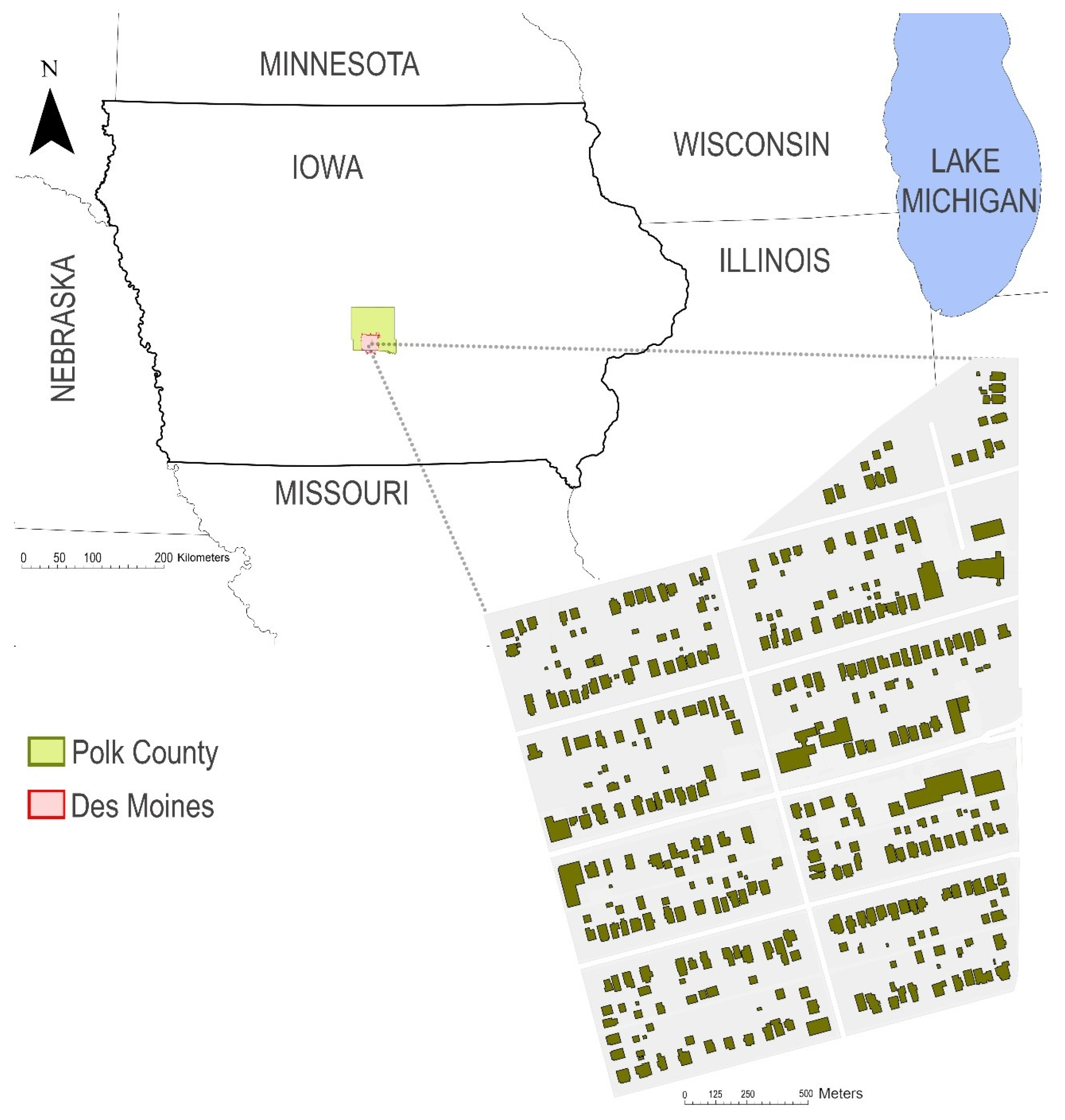
3.1. Case Study

The city of Des Moines, located in the central part of Iowa, serves as the state capital. It falls within the Cold-Humid climate zone (5A) as defined by the International Energy Conservation Code (IECC), characterized by harsh winters and hot, humid summers (Figure 1). On the east side of Des Moines (41.6° N latitude and 93.6° W longitude), the Capitol East neighborhood stands out due to its unique socio-economic characteristics and challenges, making it a representative case for many mid-sized U.S. neighborhoods. Covering approximately 282,778 square meters, Capitol East primarily consists of single-family residences constructed in the early 1900s. Much of this aging housing stock lacks proper insulation, featuring poorly sealed building envelopes with low thermal resistance (R-values) and older single-glazed windows, which contribute to inefficient energy performance. The neighborhood’s built environment, socio-economic context, and climatic extremes make it an ideal case for examining the intersection of urban heat effects and energy performance in resource-constrained settings. The following section details the steps in the methodology.

3.2. Future Weather Data Generation

The first step in the workflow involves creating future weather scenarios using TMY datasets, with the latest version, TMY3, obtained from the Des Moines International Airport—the closest weather station to the Capitol East Neighborhood—serving as the baseline. Future weather files for the years 2050 and 2080 were generated by modifying the TMY3 data through a statistical downscaling approach using CCWorldWeatherGen, a free and open-source weather generator developed by the University of Southampton [56]. This Microsoft Excel-based tool employs the “morphing” technique, a widely used method initially introduced by [70], to modify historical weather data based on projected climate shifts. The morphing process involves two key adjustments: “shifting” and “stretching”. The shifting process modifies the average monthly values of climate variables while maintaining their variability, whereas stretching adjusts the variability itself while keeping the average constant. When applied to temperature, this method not only alters the mean temperature values but also modifies the daily fluctuations by proportionally expanding or contracting diurnal variations [71].

CCWorldWeatherGen is based on the Hadley Centre Coupled Model, version 3 (HadCM3) [72], a global climate model widely used for long-term climate projections. For this study, the SRES A2 scenario was chosen, as it aligns closely with the Representative Concentration Pathway (RCP) 8.5, often considered a worst-case scenario in climate projections. RCP 8.5 represents a high-emission trajectory characterized by continued fossil fuel dependence, minimal climate mitigation, and an anticipated radiative forcing of 8.5 W/m² by 2100. This scenario was selected to assess the upper-bound impacts of climate change on urban energy demand, capturing the most severe potential temperature increases. While intermediate scenarios, such as RCP 4.5 and RCP 6.0, offer alternative mitigation pathways, RCP 8.5 remains widely used in climate impact studies due to its alignment with observed emission trends and its ability to highlight potential worst-case outcomes. Overall, the RCP framework serves as a critical tool for climate modeling, offering multiple greenhouse gas emission pathways to project future climate conditions and their potential implications [73].

3.3. Urban Heat Island Simulation

At this step, a detailed 3D model of Capitol East, previously developed in [74,75], was integrated into the UWG environment using a plugin called Dragonfly, following the workflow described in Hashemi et al. [76]. Developed by Ladybug Tools [77], the Dragonfly plugin for Grasshopper 3D enables the use of UWG within the Rhino 3D software, version 7. The model was created using a comprehensive inventory of 1142 trees (including both yard and street trees) and 272 buildings in the neighborhood. Based on data obtained from the Polk County Assessor website [78], 87 buildings were identified as having active air conditioning, operating both cooling and heating systems year-round, while 185 buildings relied on natural ventilation, equipped with heating systems only and no cooling. The assessor data includes key information about the neighborhood’s buildings, such as parcel numbers, construction materials, and the number of stories.

Table 1. Urban morphology and surface characteristics used in the UWG model.

Parameter	Input Value
Average building height	5.1 m
Footprint density	0.15
Facade-to-site ratio	0.19
Tree coverage ratio	0.35
Grass coverage ratio	0.43
Traffic intensity (W/m2)	12.5 (Low-traffic residential areas [80])
Vegetation albedo	0.2
Terrain albedo	0.18
Daytime boundary–layer height (m)	600

provides a summary of the main inputs used in the UWG simulation [79].

Buildings were further grouped according to their construction properties into 14 unique templates: 6 templates for air-conditioned buildings and 8 for naturally ventilated buildings. These templates represent varying numbers of buildings, ranging from a single building to a maximum of 69 buildings per template (

Table 2. Material properties, thermal characteristics, and key building system parameters used in the UBEM.

Category	Layers		d [m]	λ [W/mK]	R [m2K/W]
Façade Materials	Asbestos	Concrete	0.07	0.74	2.12
		Polystyrene	0.05	0.03
		Cement Plaster	0.2	0.72
		Gypsum Board	0.013	0.16
	Brick	Brick	0.15	1.02	1.98
		Polystyrene	0.05	0.03
		Air Layer	0.02	0.139
		Gypsum plaster	0.015	0.56
	Composite	Composite	0.07	0.85	2.00
		Polystyrene	0.05	0.03
		Cement	0.2	1.15
		Gypsum Board	0.013	0.16
	Wood siding	Hardwood	0.013	0.16	3.48
		OSB Board	0.013	0.91
		Hardwood	0.02	0.16
		Polystyrene	0.05	0.03
		Fiberglass	0.065	0.043
		Gypsum Board	0.013	0.16
	Metal siding	Metal	0.002	45.3	2.78
		Polystyrene	0.05	0.03
		Hardboard	0.013	0.105
		Steel	0.002	45.3
		Fiberglass	0.039	0.043
		Gypsum Board	0.013	0.16
	PVC	PVC	0.07	0.2	2.38
		Polystyrene	0.05	0.03
		Cement Plaster	0.2	0.72
		Gypsum Board	0.013	0.16
	Stucco	Stucco	0.022	0.346	2.72
		Steel	0.002	45.3
		Polystyrene	0.05	0.03
		Steel	0.002	45.3
		Fiberglass	0.039	0.043
		Gypsum Board	0.013	0.16
	Cement	Cement plaster	0.02	0.72	2.05
		Polystyrene	0.05	0.03
		Cement plaster	0.2	0.72
		Gypsum Board	0.013	0.16
Roof Material	Asphalt Shingle	Asphalt shingle	0.02	1.15	4.08
		Plywood panels	0.02	0. 11
		Fiberglass	0.15	0.043
		Softwood	0.04	0.13
		Gypsum board	0.013	0.16
Exterior Floor	Mass Floor	Carpet	0.013	0.045	1.49
		Concrete reinforced	0.15	2.15
		Polystyrene	0.034	0.03
Windows	Window to Wall (WWR) Ratio		40%
	Window Structure		Single Glazing
Building Systems	Equipment Power Density		4.43 W/m2
	Illuminance Target		350 lux
	Lighting Power Density		3.28 W/m2
DHW System	Efficiency		70%, powered by natural gas
	Water Supply Temperature		55 °C
	Water Inlet Temperature		10 °C
HVAC System	Cooling Setpoint		26 °C, powered by electricity
	Heating Setpoint		20 °C, powered by natural gas

). The meteorological data were obtained from three sets of weather data: TMY3 (simply referred to as current hereafter), and the future TMY scenarios for 2050 and 2080, created in the previous step. The resulting weather files, labeled ‘Current + UHI’, ‘2050 + UHI’, and ‘2080 + UHI’, were formatted in EnergyPlus Weather (EPW) and served as key inputs for the subsequent phases of the workflow.

3.4. Urban Building Energy Modeling (UBEM)

To simulate urban-scale energy performance, this study utilized the Urban Modelling Interface (UMI), a Rhinoceros-based urban energy modeling tool that integrates geometric, material, and environmental data to assess neighborhood-level energy demand [81]. The UMI employs intricate urban shadow calculations and an EnergyPlus simulation engine to predict thermal loads at the city scale. The modeling process involved multiple data sources and refinement steps to ensure a detailed and realistic representation of the built environment.

The 3D geometry of the Capitol East neighborhood in Des Moines, Iowa, was developed in Rhinoceros 3D using GIS data from the City of Des Moines. Building footprints were extruded to roof elevations from GIS records, but due to variations in roof heights and partial second stories, floor plans from the Polk County Assessor’s database were used to refine individual structures. This step was critical, as the UMI evaluates thermal loads based on a building’s total insulated volume, making precise height representation essential for accurate energy simulations.

Beyond physical geometry, detailed building attributes were integrated to enhance thermal performance modeling. The assessor data provided essential inputs, including the construction year, number of stories, insulation quality, HVAC system type, and number of residential units. An identification system based on parcel numbers allowed for seamless cross-referencing between the Rhino-UMI model and assessor records, ensuring that each building was assigned appropriate thermal and operational properties. To further refine the simulation, a high-resolution residential occupancy schedule was incorporated, addressing the limitations of static occupancy assumptions in traditional energy models. A Markov chain-based model combined with American Time-Use Survey (ATUS) data was used to generate stochastic, time-dependent occupancy schedules, which were further refined using local survey data to match the energy use patterns of the neighborhood [82]. Additionally, urban vegetation was modeled with detailed canopy and trunk characteristics, obtained from a comprehensive urban tree inventory conducted by the research team, capturing shading effects that influence cooling demand [75].

To align with the economic and historical characteristics of the study area, it was assumed that none of the air-conditioned buildings included energy economizers or heat recovery systems. This assumption was based on two key factors: first, the general economic conditions of the neighborhood, which suggest that such efficiency upgrades are unlikely; and second, the average retrofit age, which was around 1980 according to the assessor’s data.

Among the 272 buildings modeled, 87 had air conditioning, meaning they were equipped with both heating and cooling systems, relied on mechanical ventilation (AC) and scheduled ventilation, and did not utilize natural ventilation. The remaining 185 buildings did not have air conditioning, meaning they lacked a cooling capability entirely, had no mechanical or scheduled ventilation, and relied solely on natural ventilation. This assumption was made due to the lack of available data on potential alternative cooling systems in the assessor’s records, which did not specify whether occupants had installed other means of cooling. Regardless of cooling availability, all 272 buildings were equipped with heating systems fueled by natural gas, as indicated by the assessor’s records.

Table 2 summarizes the building template specifications, with façade materials and window properties derived from assessor data, while other assumptions were adopted from ASHRAE Standard 90.1. Based on assessor data, the majority of residential buildings were initially categorized into primary façade materials of metal siding, mixed materials (36.18%), PVC (19.34%), and hardboard (17.29%). However, to improve the accuracy of thermal modeling, these classifications were refined into eight façade material clusters: asbestos, brick, composite, wood siding, metal siding, PVC, stucco, and cement. Each building in the model was assigned one of these façade templates based on its parcel ID, using a structured cross-referencing system. The parcel number served as a unique identifier that linked individual building records from the assessor database with the Rhino-UMI model. This allowed for the seamless integration of façade classification, ensuring that each structure’s thermal properties reflected its documented construction type. Given the lack of explicit insulation data in the assessor records, a standardized approach was adopted based on the dominant construction practices of the era. As most structures in the neighborhood were built before 1980, polystyrene insulation was applied uniformly across all templates, reflecting its widespread use in residential buildings of that period. The assumption was necessary to maintain model consistency and prevent excessive variation stemming from unverified retrofit data.

4. Results and Discussion

4.1. Simulation Reliability

Ensuring the reliability of weather and energy simulations is essential for producing credible results. While direct validation using measured data was not conducted, the models used in this study have been widely applied and validated in prior research.

For UHI modeling, the UWG has been extensively validated in previous studies, demonstrating its capability to simulate urban climate effects by integrating urban morphology, vegetation, and building characteristics [51,52,53]. In addition, CCWorldWeatherGen, based on the Hadley Centre’s HadCM3 model, has been utilized in multiple climate studies to generate future weather scenarios and is recognized as a reliable tool for downscaling climate projections [83].

For UBEM, the UMI has been validated in research comparing its results with the U.S. Department of Energy (DOE) reference building prototypes. Findings from [84] confirm that UMI-based simulations closely align with DOE’s IDF-based models. Their study utilized the same UMI modeling approach as this study, developing a 3D model in UMI based on the DOE prototype for single-family residential structures and comparing results from UMI and direct EnergyPlus simulations using DOE reference buildings. Despite differences in window modeling and thermal zoning approaches, the resulting energy use metrics were insignificantly different. Under identical geometry, thermal characteristics, and environmental conditions, the cooling loads for both models remained consistent, reaffirming the reliability and accuracy of the same modeling framework applied in this study. The DOE reference prototypes, as validated energy models, serve as a benchmark for building performance assessment.

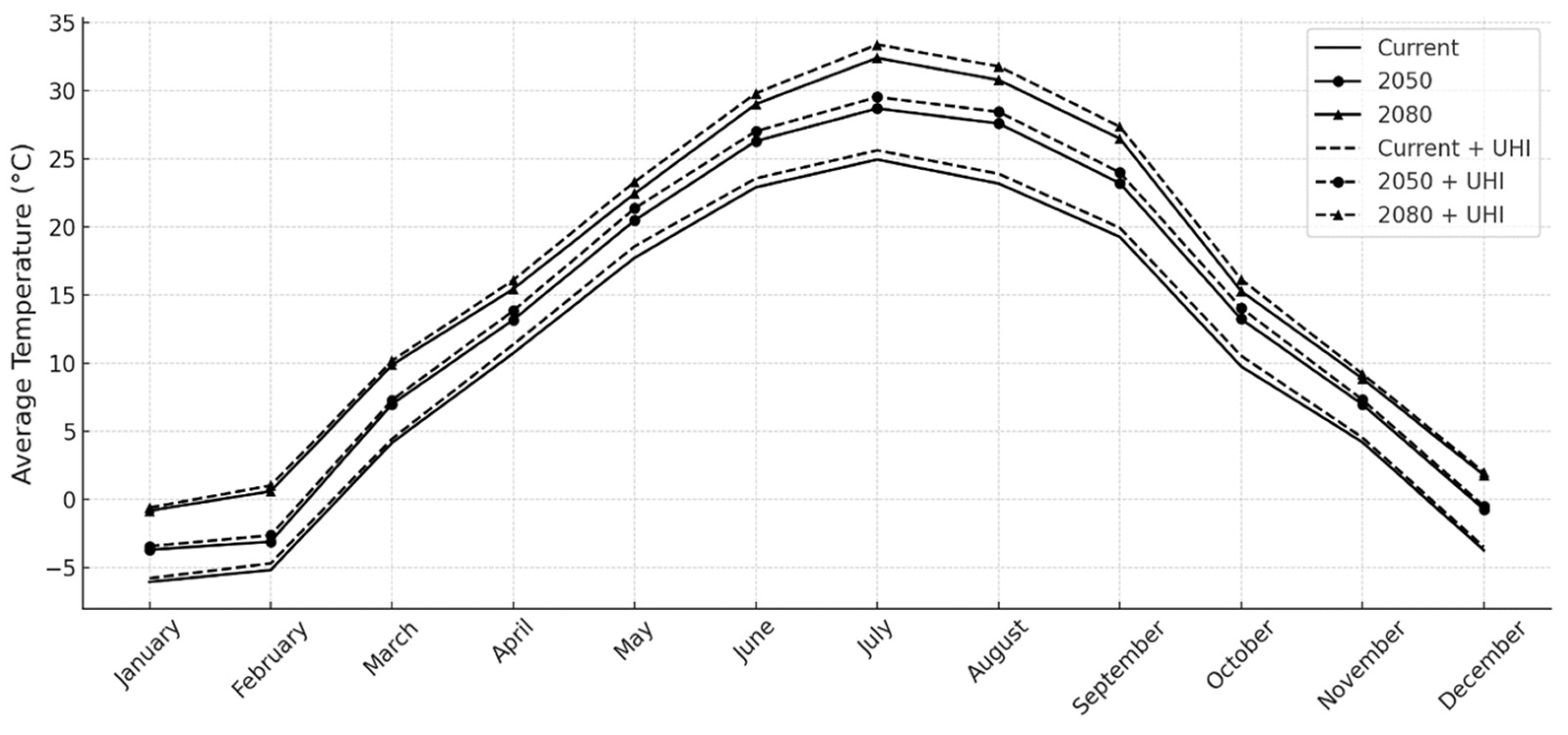
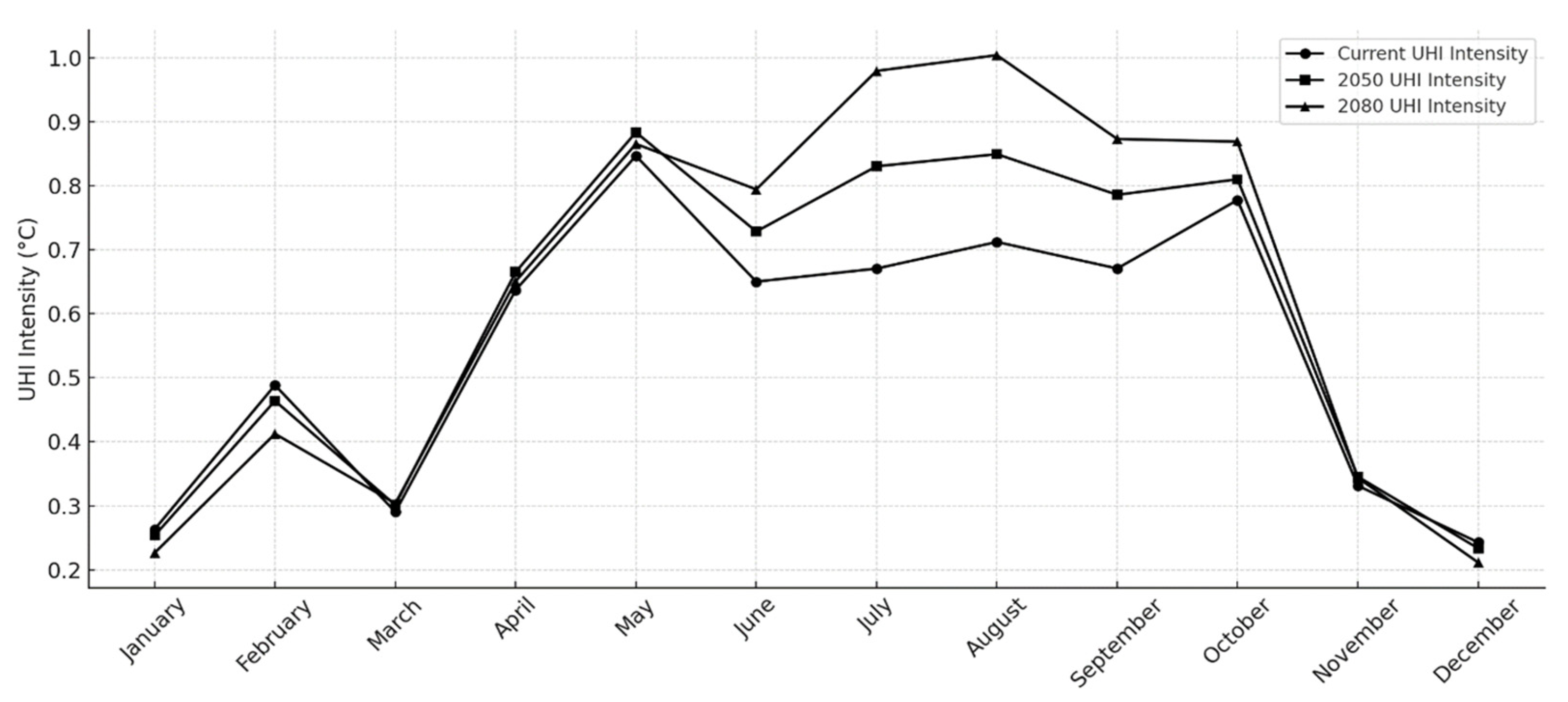
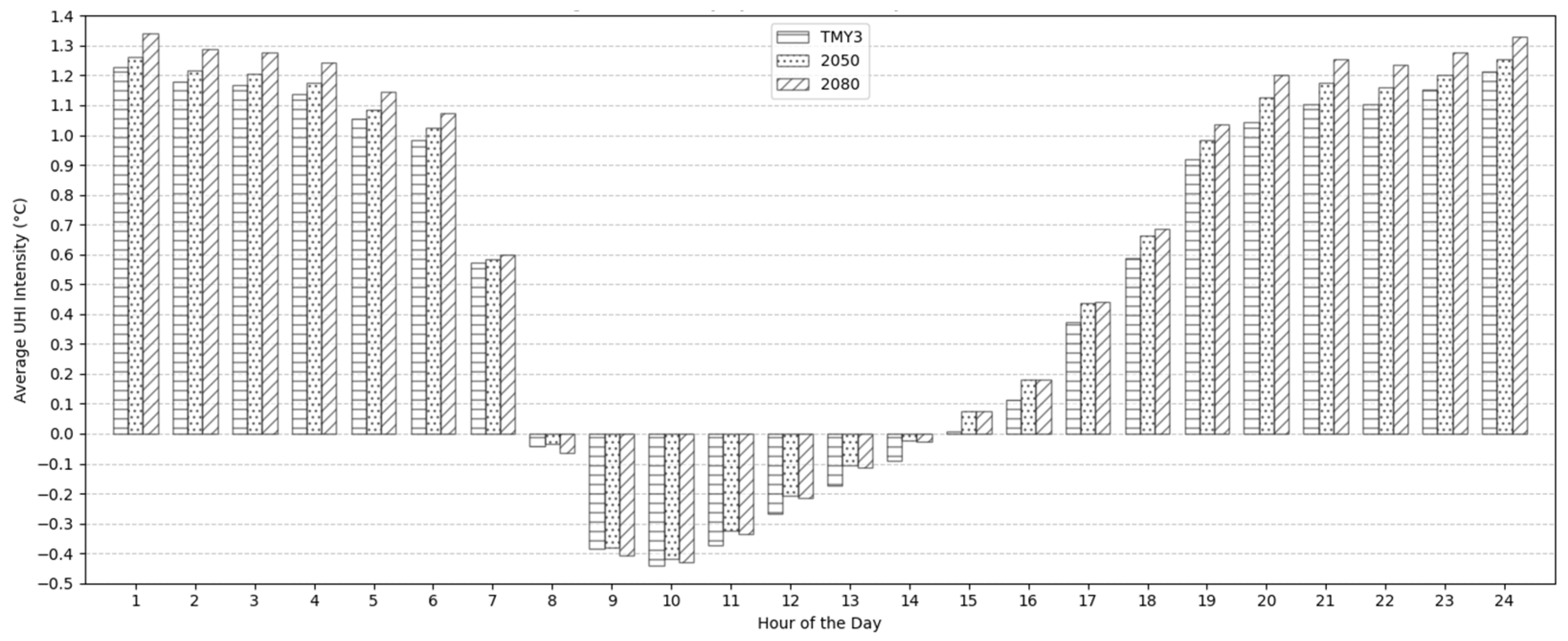
4.2. Future Projected and UHI-Induced Temperature

Using current data as a baseline, significant temperature shifts are projected for 2050 and 2080, highlighting a consistent warming trend over time. Each month’s average temperature shows a significant increase compared to the current baseline, with the warming trend becoming more pronounced by 2080 (Figure 2). January, the coldest month, has an average temperature of −6.04 °C in current conditions, rising to −3.68 °C in 2050 and further to −0.81 °C in 2080 (a total increase of 5.23 °C). July, the warmest month, has an average temperature of 23.20 °C in current conditions, increasing to 27.61 °C in 2050 and to 30.79 °C in 2080, marking a total rise of 7.59 °C.

Seasonal analysis reveals that summer (June–August) experiences greater absolute warming compared to winter (December–February). The average winter temperature increases from −5.16 °C in current conditions to −3.09 °C in 2050 and further to 0.62 °C in 2080, showing a total rise of 5.78 °C. By comparison, the average summer temperature increases from 23.20 °C in current conditions to 27.61 °C in 2050 and further to 30.79 °C in 2080, a total rise of 7.59 °C.

Similar projections have been observed in Philadelphia’s urban climate modeling, where morphing techniques applied to future weather data indicated persistent warming across all months, with the highest absolute increases occurring during summer [71]. The elevated temperatures in warmer months intensify urban heat retention, compounding the risk of extreme heat events in cities with comparable climatic conditions. In addition, it reflects the increasing dominance of radiative forcing and the reduced efficiency of evaporative cooling in urban areas, a pattern observed in climate projections for Toronto, Canada, where morphing-based future climate files, including those generated through CCWorldWeatherGen, similarly indicated stronger warming in summer than in winter [85].

When UHI effects were added to current and future weather scenarios, additional warming was observed across all scenarios, averaged over the months. For instance, in January, the Current + UHI temperature registers −5.78 °C, which is 0.26 °C warmer than the current baseline of −6.04 °C. In the future scenarios, January temperatures under UHI effects rise to −3.43 °C in 2050 + UHI, an increase of 0.25 °C compared to the 2050 baseline, and to −0.58 °C in 2080 + UHI, which is 0.23 °C higher than the 2080 baseline. Warmer months show a slightly larger UHI-induced increase. For example, the Current + UHI temperature in July is 23.91 °C, which is 0.71 °C warmer than the current baseline of 23.20 °C. The corresponding UHI-adjusted temperatures for July in 2050 and 2080 are 28.46 °C, an increase of 0.85 °C compared to the 2050 baseline, and 31.79 °C, which is 0.99 °C higher than the 2080 baseline.

The UHI intensity was calculated as the temperature difference between “+UHI” scenarios and their respective baselines using the below formula:

UHI Intensity = T_{weather scenario +UHI} − T_{weather scenario}

(1)

Figure 3 illustrates the monthly average intensities for three weather scenarios.

The annual average UHI intensity demonstrates a clear progression across the three scenarios. In the current scenario, the annual average UHI intensity is approximately 0.55 °C, representing the baseline level of urban heating under existing conditions. By 2050, this value increases to 0.60 °C and reaches 0.63 °C in 2080. Seasonal analysis consistently indicates that UHI intensity is highest in the summer months, particularly in August, which shows the peak average in all scenarios.

In the current scenario, August reaches 0.71 °C, while the lowest UHI intensities occur in winter, with December averaging 0.24 °C. Spring and fall record average UHI intensities of 0.64 °C and 0.49 °C, respectively. By 2050, UHI intensity increases slightly across all months, with August peaking at 0.85 °C and December remaining the lowest at 0.23 °C. Spring and fall show average UHI intensities of 0.66 °C and 0.46 °C, respectively. By 2080, UHI intensities intensify further, with August reaching 1.00 °C and December declining slightly to 0.21 °C. Spring and fall record averages of 0.65 °C and 0.41 °C, respectively. These findings support the expectation that climate change will amplify urban heat stress, particularly during warm months, as UHI effects compound the impact of rising temperatures [85]. A similar warming pattern was observed in large-scale UHI analyses across North American cities, where daytime UHI intensities are more pronounced in humid regions like the Midwest and Eastern U.S. due to reduced convective cooling efficiency [86]. This is reflected in the projections, as the greater summer warming suggests that cities in humid regions will face increased heat stress from both climate change and urban heat retention.

However, the interaction between climate change and UHI effects is complex and not a simple linear increase. Some projections indicate that rising atmospheric temperatures may weaken urban-rural contrasts at night, leading to reduced nocturnal UHI intensities in future scenarios. Conversely, higher background temperatures during the day—particularly in summer—limit urban cooling efficiency, sustaining UHI effects despite overall warming [87]. The results presented here affirm this trend, with August UHI intensities increasing from 0.71 °C in the current scenario to 1.00 °C by 2080, highlighting the amplification of daytime heat retention in urban areas. However, some studies suggest a potential weakening of winter UHI due to a diminishing urban–rural temperature gradient. Despite this, the simulations indicate only a minor reduction in December UHI intensity, from 0.24 °C (current) to 0.21 °C (2080). Although seasonal variations persist, the overall trajectory of UHI intensity remains upward—particularly in warm months—as climate change exacerbates urban heat stress.

Shifting to a daily analysis, UHI intensity increases noticeably in the late afternoon as urban surfaces release the heat absorbed during the day. The intensities peak during nighttime, specifically around midnight, with the highest values recorded between 23:00 and 1:00 (Figure 4). These values were calculated on a year-round basis. In the current scenario, the UHI intensity reaches a maximum of 1.23 °C at 1:00, slightly decreasing afterward. Similarly, in the 2050 and 2080 scenarios, the peak intensities occur at midnight, with values of 1.26 °C and 1.34 °C, respectively, reflecting the increasing impact of warming trends over time.

During the early morning hours, UHI intensities begin to decline steadily, transitioning into UCI conditions shortly after sunrise. In all scenarios, the UCI effect becomes evident around 8:00, with the temperature difference between the weather scenarios and their UHI-induced conditions becoming negative. The lowest intensities are recorded between 9:00 and 11:00, with peak values of −0.39 °C, −0.38 °C, and −0.41 °C in the current, 2050, and 2080 scenarios, respectively. As the day progresses, the intensity shifts back toward positive values as urban surfaces reheat. This transition occurs consistently at 15:00 across all scenarios, reflecting a balance between heat absorption and cooling throughout the day. The intensities continue to rise steadily through the evening, completing the daily UHI cycle. The presence of a morning UCI effect has been widely documented in various urban environments, where synoptic conditions and thermal storage differences between urban and rural areas influence cooling patterns. In Melbourne, Australia, early-morning UCI effects have been observed, attributed to lower heat retention in urban areas under specific atmospheric conditions [17]. Similarly, research in Hong Kong indicated that low-rise, low-density urban areas experienced a stronger UCI effect compared to high-density regions, largely due to lower thermal storage and reduced nighttime heat retention [88]. The findings here reflect a similar trend, suggesting that urban morphology and atmospheric factors influence early-morning cooling patterns, reinforcing the complexity of daily temperature dynamics in urban areas.

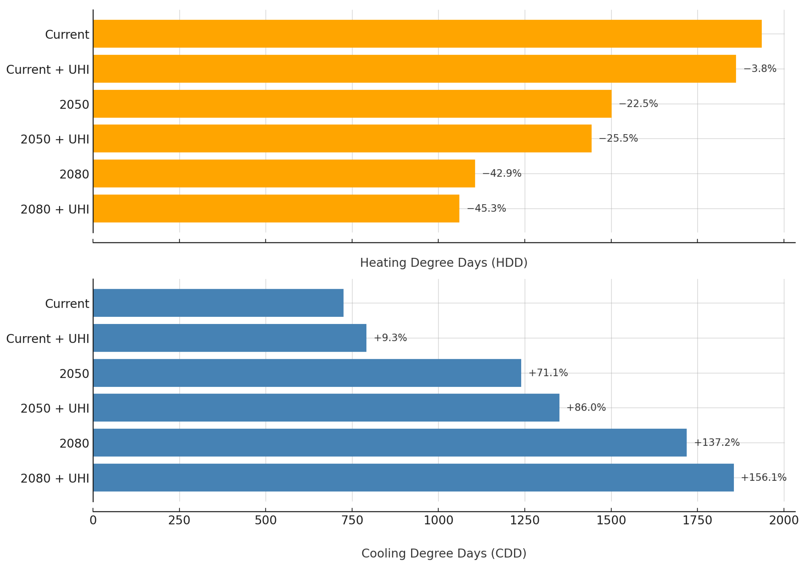
4.3. Degree Days Change Due to Climate Change and the UHI

Degree days are commonly utilized as a rough estimation of heating and cooling demands [89]. Heating Degree Days (HDDs) and Cooling Degree Days (CDDs) were calculated across six weather scenarios using the standard methodology outlined in ASHRAE (2017). HDDs and CDDs are calculated as the sum of the differences between daily average temperatures and the base 10 °C (50 °F) or 18.3 °C (65 °F). When the outdoor temperature is below (or above) the base temperature, heating (or cooling) systems are required to operate, and therefore deviations result in increased energy requirements. The formulas for HDDs and CDDs are as follows:

$$HDD={\sum }_{i=1}^N{(10.0 °\mathrm{C}-{\stackrel{—}{\mathrm{T}}}_{\mathrm{i}})}^{+}$$

(2)

$$CDD={\sum }_{i=1}^N {({\stackrel{—}{\mathrm{T}}}_{\mathrm{i}}-18.3 °\mathrm{C})}^{+}$$

(3)

where N is the number of days in a year, 10 °C and 18.3 °C are the base temperatures for HDD and CDD calculations, respectively. T_i is the mean daily temperature, determined by averaging the daily maximum and minimum temperatures. The + superscript indicates that only positive values within the bracketed expressions are summed.

In the current scenario, the HDDs are 1934 °C days, while the CDDs are 7120 °C days, indicating that the baseline climate is heating-dominated (Figure 5). However, HDDs show a clear decreasing trend from the current scenario to future scenarios, beginning with a 3.8% reduction when UHI effects are added to this scenario. In the 2050 scenario, HDDs decrease further by 22.5% compared to the current scenario, while the inclusion of the UHI effect amplifies this reduction to 25.5%. By 2080, the decrease becomes even more pronounced, with a 42.9% reduction without the UHI and a 45.3% reduction with the UHI.

In contrast, CDDs exhibit a substantial increase over time, starting with a 9.3% rise when moving from the current scenario to the current scenario with the UHI. In the 2050 scenario, CDDs increase further by 71.1% relative to the current scenario, and the UHI effect intensifies this rise to 86.%. The trend becomes even more dramatic by 2080, with CDDs increasing by 137% without the UHI and 156.1% with the UHI. Several studies support the observed trends in this research regarding HDD reductions and CDD increases due to UHI effects and future climate projections. Schatz and Kucharik [90] examined a densely built area in Madison, Wisconsin, where stronger UHI effects led to a 6% HDD decrease (260–302 fewer HDD) and a 23–29% CDD increase compared to rural areas, underscoring the influence of urban density on energy demand. In contrast, this study focuses on a low-rise neighborhood with milder UHI effects, explaining the relatively smaller changes observed. Ramon et al. [91] projected a 27% HDD decline (from 3189 to 2337 HDDs) and a 2.4-fold CDD increase (from 167 to 401 CDDs) for 2070–2098 under the RCP 8.5 scenario in Belgium, highlighting substantial future climate impacts. Despite differences in urban form, background climate, and methodology, both studies reinforce the expectation of declining HDDs and rising CDDs due to microclimate and climate change.

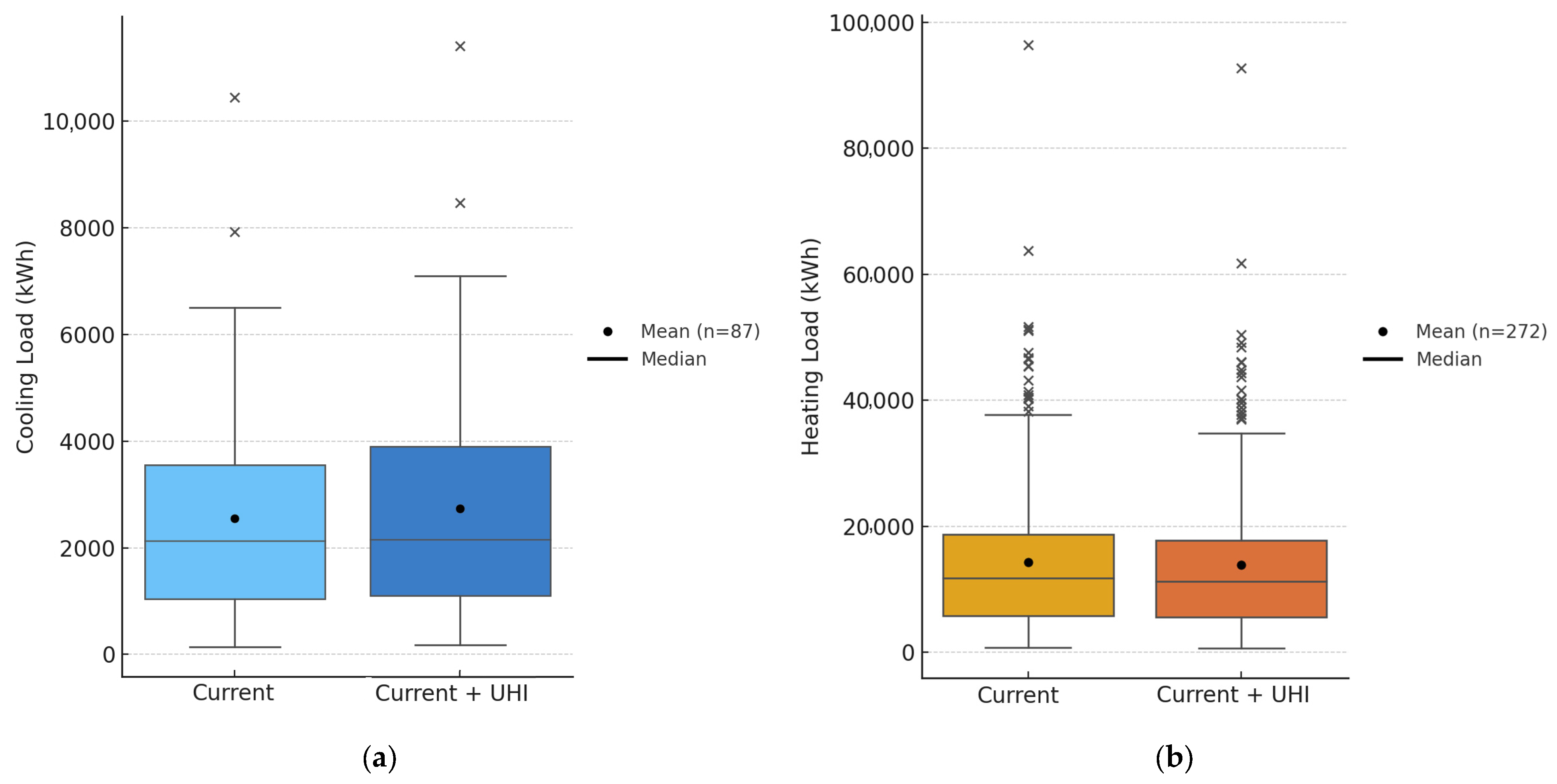
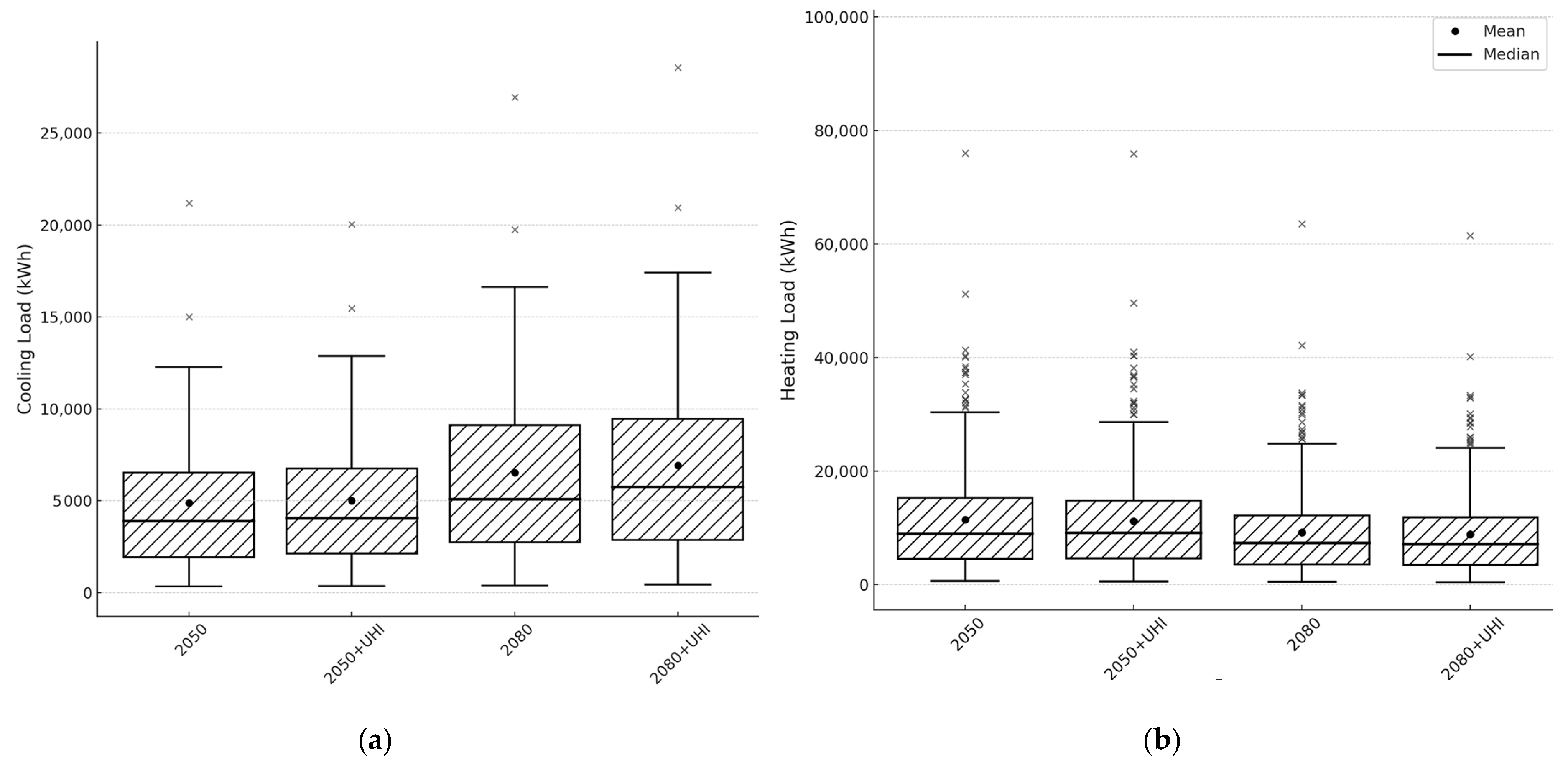
4.4. Impacts on Cooling and Heating Loads

The analysis of cooling and heating loads under the baseline and UHI-influenced scenarios provides key insights into the impact of localized warming. Figure 6a illustrates the cooling demand of all buildings across the neighborhood in these two conditions (current and current + UHI). For cooling loads, the mean (median) demand increases from 2551 kWh (2127 kWh) in the baseline scenario to 2733 kWh (2151 kWh) in the UHI-influenced scenario, representing a 7.1% (1.1%) increase. This underscores the additional cooling burden imposed by urban heat effects on buildings when integrated into the current TMY3 dataset.

The minimum cooling load rises from 147 kWh in the baseline to 182 kWh under UHI conditions, marking a 23.8% increase. Even buildings with the lowest cooling requirements experience a substantial rise due to the added heat introduced by the UHI. Similarly, the maximum cooling load (excluding outliers) increases from 6500 kWh to 7094 kWh, reflecting a 9.1% increase. Additionally, the interquartile range (IQR) expands from 2500 kWh to 2784 kWh, an 11.3% increase that highlights greater variability in cooling loads. This underestimation highlights the significant role of site-specific climatic conditions in driving cooling energy needs, particularly in urban neighborhoods where building arrangements and heat-retaining surfaces intensify thermal loads.

Conversely, for heating loads (Figure 6b), the mean (median) demand decreases from 14,260 kWh (11,793 kWh) in the baseline scenario to 13,877 kWh (11,225 kWh) in the UHI-influenced scenario, representing a 2.7% (4.8%) decrease. The minimum heating load drops from 724 kWh in the baseline to 702 kWh under UHI conditions, marking a 3.0% decrease. Similarly, the maximum heating load (excluding outliers) decreases from 37,682 kWh to 34,736 kWh, reflecting a 7.8% reduction. Additionally, the IQR decreases from 12,984 kWh to 12,157 kWh, a 6.4% drop that highlights reduced variability in heating loads across the neighborhood. The UMI calculates heating loads in kWh using EnergyPlus, regardless of fuel type. If required, EnergyPlus separately calculates fuel consumption based on system efficiency, but the UMI consistently reports heating demand in kWh to ensure uniformity across different energy sources. Overall, the UHI effect increased cooling energy requirements by 7.1% while reducing heating demands by 2.7% on average across the neighborhood.

Expanding the analysis to future scenarios and their UHI-influenced counterparts, Figure 7 illustrates the shifts in cooling (left) and heating (right) across four scenarios. In the 2050 scenario, the average cooling load increases to 4894 kWh, a 91.8% rise from current conditions, and with UHI effects included, it further increases to 5001 kWh, reflecting a total rise of 96.0%. By 2080, the average cooling load increases to 6519 kWh (155.6%) compared to the baseline, peaking at 6915 kWh (171.1%) in the UHI-influenced 2080 scenario. These results highlight the substantial increase in cooling demand driven by rising temperatures and the compounded effects of urban heat. Similarly, Deng et al. [92] demonstrated that climate change could drive a substantial increase in cooling energy use, with projections ranging from 113% to 173% in urban residential neighborhoods by 2050 under high-emission scenarios (SSP5-8.5, SSP3-7.0). Tootkaboni et al. [85] reported even greater increases of up to 255.1% in residential buildings under extreme climate change scenarios (RCP 8.5, 2081–2099), particularly in single-family houses due to their high shape factor and exposure to outdoor temperature fluctuations. However, lower estimates have been reported under different climate projection frameworks. Shen et al. [93] projected a more moderate increase in cooling demand, ranging from 2.6% to 24% across U.S. residential buildings for the period 2040–2069 under the SRES A2 and A1FI scenarios. The discrepancy is primarily due to differences in climate modeling frameworks. While the newer SSP and RCP scenarios (e.g., RCP 8.5, SSP5-8.5) account for higher greenhouse gas emissions and more severe warming trajectories, the SRES A2 and A1FI scenarios are based on older projections that assume different economic, technological, and emissions pathways.

In contrast, heating loads exhibit a consistent decline across all future scenarios, reflecting reduced energy demand due to warming and the UHI effect. By 2050, the average heating load decreases to 11,433 kWh (−19.8%) compared to the baseline, and with UHI effects included, it further declines to 11,209 kWh (−21.4%). By 2080, the average heating load drops significantly to 9182 kWh (−35.6%), reaching 8885 kWh (−37.7%) under UHI conditions. This trend aligns with previous studies projecting reductions in heating demand. Tootkaboni et al. [85] estimated a 30.9% decrease in heating demand across Milan’s residential buildings by 2081–2099 under RCP 4.5 and RCP 8.5. Similarly, Deng et al. [92] projected a 22–31% reduction in Geneva’s residential neighborhoods by 2050 under SSP1-2.6 to SSP5-8.5. Both studies attribute these declines to rising winter temperatures, which lessen the need for space heating.

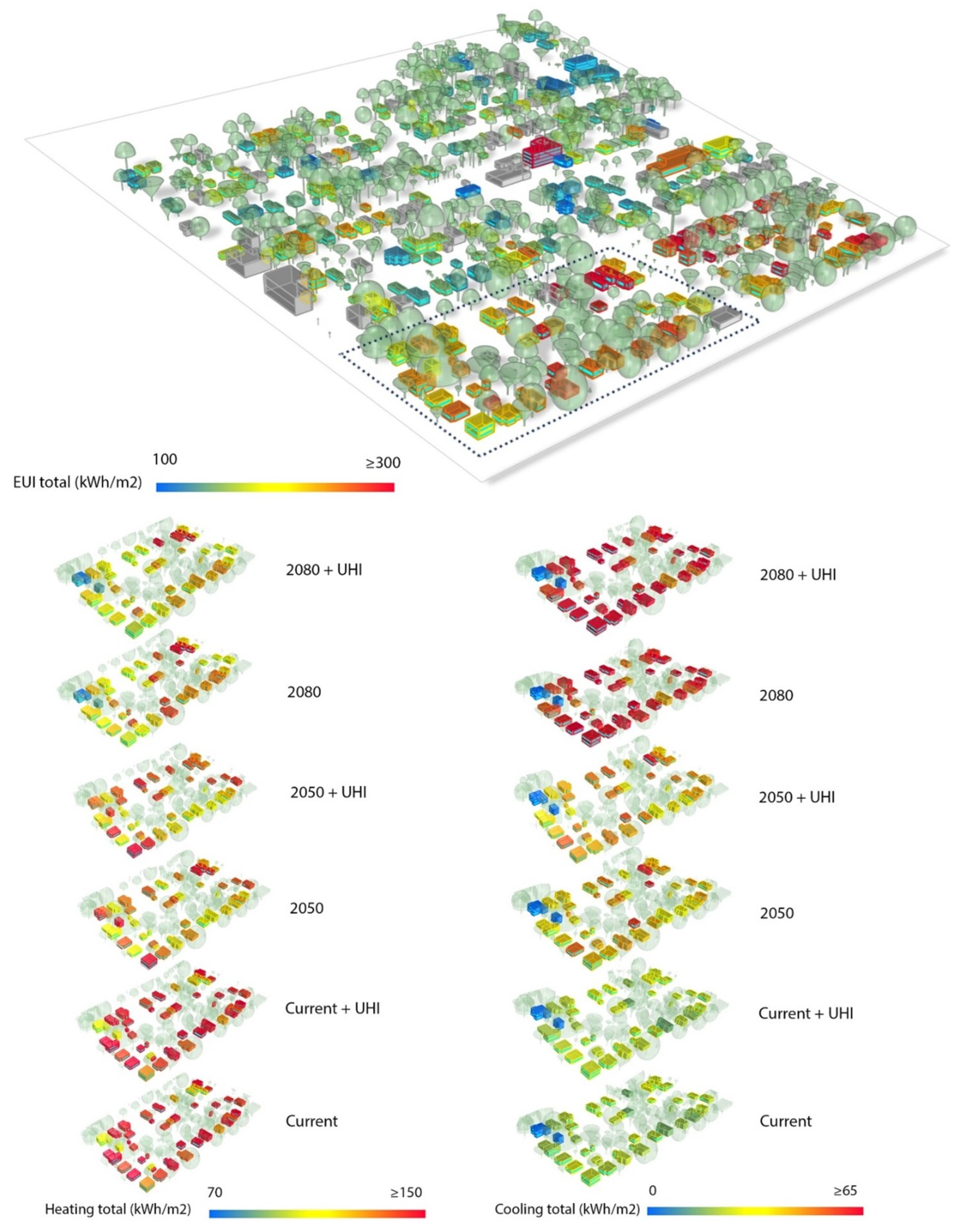
4.5. Impacts on Energy Use Intensity Changes (EUI)

Energy Use Intensity (EUI) measures energy consumption per unit area (kWh/m²), allowing for direct comparisons across buildings of different sizes. Figure 8 illustrates heating and cooling EUI trends across the six weather scenarios, highlighting a sharp upward shift in cooling demand and an inverse trend for heating. Under current conditions, the mean cooling EUI across the neighborhood is 21.26 kWh/m², but incorporating UHI effects leads to a 6.85% increase, raising it to 22.72 kWh/m². Future climate projections indicate a dramatic rise, with cooling EUI reaching 40.61 kWh/m² by 2050, representing a 91.0% increase from current condition. When UHI effects are factored in, 2050 cooling EUI increases further to 41.55 kWh/m² (+2.3%). Deng et al. (2023) projected that cooling energy intensity in residential buildings could rise from 12 kWh/m² to 32 kWh/m² by 2050. By 2080, EUI reaches 54.03 kWh/m², marking a 33.0% jump from 2050 and a 154.1% increase from current conditions. Additionally, 2080 + UHI cooling EUI increases further to 57.38 kWh/m² (+6.2% from 2080). Likewise, Berardi and Jafarpur [94] projected that cooling EUI could increase between 15% and 126% by 2070 and Jylhä et al. [95] projected a 40–80% increase in cooling energy demand by 2100, depending on building typology and climate conditions. They highlight that factors such as insulation levels, window-to-wall ratios, and ventilation strategies significantly influence the extent of cooling demand increases.

On the other hand, EUI for heating declines across all future scenarios as temperatures rise. Under current conditions, the mean heating EUI is 135.40 kWh/m², decreasing by 2.67% with UHI effects to 131.78 kWh/m². By 2050, heating EUI drops 20.0% to 108.28 kWh/m², with 2050 + UHI further reducing it by 2.2% to 105.91 kWh/m². By 2080, heating EUI falls 20.0% more to 86.58 kWh/m², totaling a 40.1% reduction from current conditions. Factoring in UHI, 2080 + UHI decreases it by 3.1%, reaching 83.94 kWh/m². For heating EUI, Berardi and Jafarpur [94] reported heating EUI reductions of 18–33% by 2070. Jylhä et al. (2015) [95] projected heating EUI reductions of 20–40% by 2100.

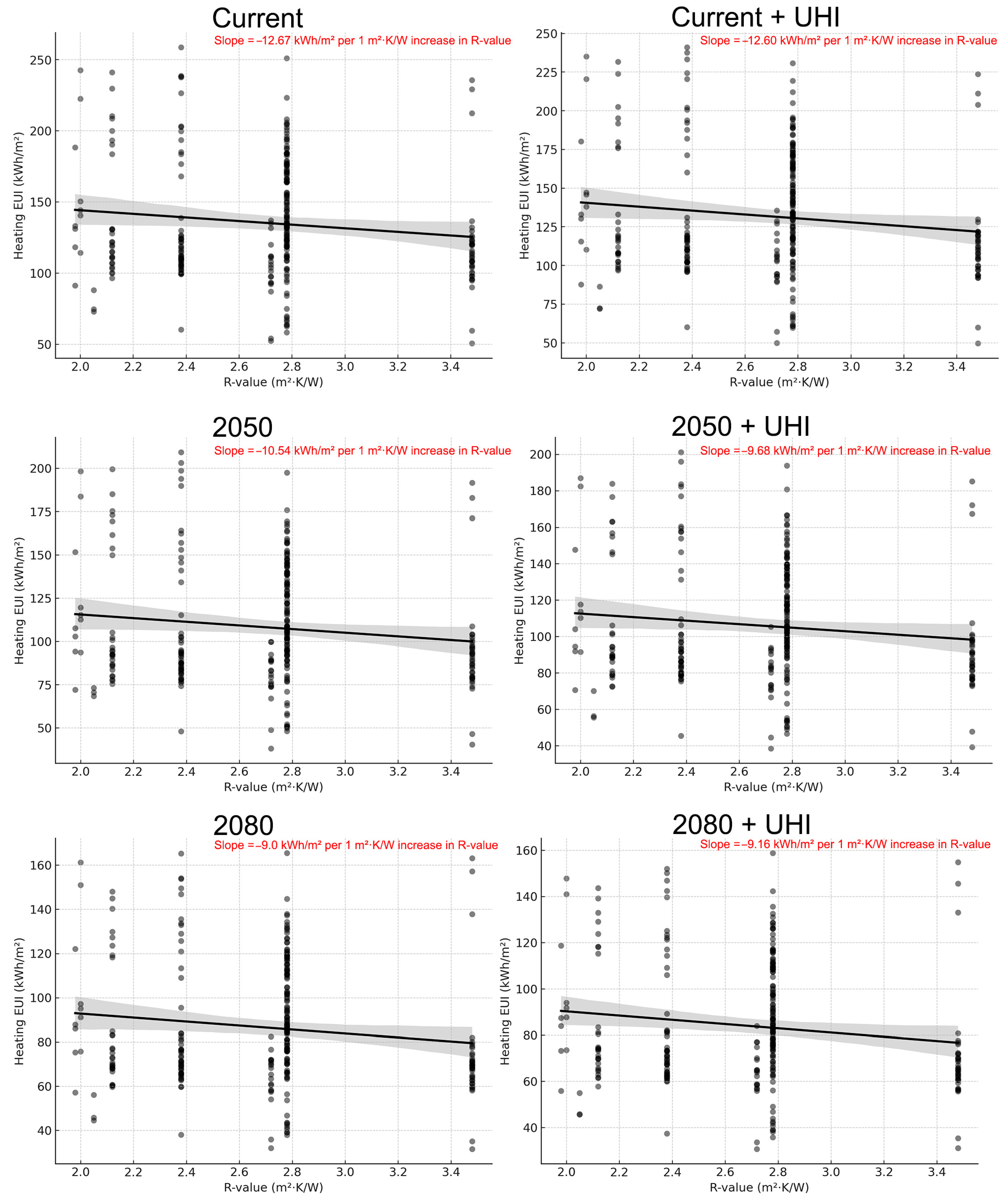
R-Value Sensitivity Analysis Across Weather Scenarios

To enable cross-comparison between building templates, the impact of R-value, which represents the thermal resistance of wall assemblies, is explored, as it represents the most noticeable difference between building templates in the dataset (see Table 2). The analysis clusters buildings by their thermal resistance (R-value) to provide a unified perspective across scenarios and building types.

Wall assemblies in building templates show notable differences in R-value, ranging from slightly higher than 2.0 m²·K/W (11 ft²·h·°F/BTU) to 3.4 m²·K/W (19.5 ft²·h·°F/BTU). Despite these differences, all buildings assessed have relatively low thermal resistance compared to the International Energy Conservation Code (IECC) requirements. For Climate Zone 5A, the IECC mandates a minimum R-value of 3.5 m²·K/W (R-20 ft²·h·°F/BTU) for cavity-only insulation or 2.3 m²·K/W (R-13 ft²·h·°F/BTU) cavity insulation plus 0.9 m²·K/W (R-5 ft²·h·°F/BTU) continuous insulation (c.i.).

The coefficient of determination, denoted as R², is a statistical measure used to evaluate the strength and proportion of the variation in a dependent variable (here, cooling or heating EUI) that can be explained by an independent variable (here, R-value). It is derived from the following formula:

$${\mathrm{R}}^2=1-{\displaystyle \frac{{\mathrm{S}\mathrm{S}}_{\mathrm{r}\mathrm{e}\mathrm{s}\mathrm{i}\mathrm{d}\mathrm{u}\mathrm{a}\mathrm{l}}}{{\mathrm{S}\mathrm{S}}_{\mathrm{t}\mathrm{o}\mathrm{t}\mathrm{a}\mathrm{l}}}}$$

(4)

where SS_residual represents the sum of squared residuals (the unexplained variance), and SS_total represents the total variance in the dependent variable.

In the context of this dataset, R² quantifies how well variations in R-value explain the differences in cooling and heating EUI across buildings under different weather scenarios. For the current scenario, the relationship between R-value and cooling EUI (Figure 9) shows a negative slope of −1.08, indicating that for every 1 m²·K/W increase in R-value, cooling EUI decreases by 1.08 kWh/m². Over the full range of R-values in the dataset, this results in a total reduction of 1.62 kWh/m². Incorporating UHI effects strengthens this negative correlation, with a steeper slope of −1.58, leading to a total reduction of 2.38 kWh/m² across the dataset’s R-value range. The enhanced cooling demand due to the UHI increases the potential impact of higher insulation levels.

Future climate projections further amplify this trend. By 2050, the cooling EUI sensitivity to R-value is slightly lower than the present climate, with a slope of −0.99, resulting in a total reduction of 1.49 kWh/m². However, under 2050 + UHI conditions, the slope becomes more pronounced at −3.51, yielding a total reduction of 5.27 kWh/m².

By 2080, the influence of the R-value intensifies, with a slope of −5.84, leading to a total cooling EUI reduction of 8.77 kWh/m² across the dataset’s R-value ranges. The 2080 + UHI scenario exhibits the steepest decline, with a slope of −6.56, bringing the largest total reduction of 9.85 kWh/m².

Although the role of R-value in reducing cooling EUI became more significant under future climate scenarios, its impact on heating EUI shows the opposite trend. As temperatures rise, the role of insulation in reducing heating demand becomes less significant, with diminishing returns in energy savings (Figure 10). For the current scenario, the relationship between R-value and heating EUI exhibits a negative slope, indicating that for every 1 m²·K/W increase in R-value, heating EUI decreases by 12.67 kWh/m². Over the full range of R-values in the dataset, this results in a total reduction of 19.01 kWh/m². Adding UHI to the current scenario slightly reduces the sensitivity of heating EUI to R-value, with a slope of −12.60, leading to a total reduction of 18.90 kWh/m².

Under the 2050 scenario, the magnitude of the impact decreases, with a slope of −10.54, resulting in a total heating EUI reduction of 15.80 kWh/m². With 2050 + UHI, the correlation weakens further, with a slope of −9.69, yielding a total reduction of 14.52 kWh/m². By 2080, the impact of insulation on heating EUI continues to diminish. The slope decreases to −9.0, bringing a total reduction of 13.51 kWh/m². In the 2080 + UHI scenario, the slope stabilizes at −9.164, leading to a total reduction of 13.75 kWh/m².

The findings indicate that the R-value will play an increasingly critical role in managing cooling loads, especially under future high-temperature scenarios where UHI effects amplify urban overheating. Higher insulation levels have been shown to reduce peak cooling loads in high-UHI environments, although their effectiveness diminishes with rising temperatures [96,97]. However, the reduced effectiveness of insulation in lowering heating loads suggests that future energy efficiency policies should focus more on passive cooling measures rather than heating efficiency improvements.

5. Conclusions

This study employed a multi-step modeling workflow integrating canopy-level UHI simulation tools and future climate modeling to assess the impact of microclimate effects and climate change on urban building energy consumption. Unlike conventional studies that rely on standardized prototypes, this research examines non-standardized, low-income residential buildings, which are more susceptible to heat stress and energy cost burdens. By integrating high-resolution urban energy modeling with future climate projections, this study provides a more granular assessment of neighborhood-scale energy demand fluctuations, addressing critical gaps in previous research.

The findings underscore the urgent need for climate-adaptive building policies as cooling demand increases and heating requirements decline, irrespective of emission scenarios. The growing reliance on air conditioning is projected to elevate electricity consumption and strain peak energy supplies, potentially leading to grid instability during high-demand periods. To address these challenges, it is imperative to implement integrated urban energy policies that promote energy efficiency, building retrofits, and demand–response strategies to balance future energy loads effectively.

High-emission climate pathways could exacerbate cooling energy burdens, reinforcing the necessity for adaptive urban planning and passive design strategies. Enhancements to building codes, such as the International Energy Conservation Code (IECC) and ASHRAE Standard 90.1, should incorporate provisions for improved insulation, reflective roofing materials, and advanced HVAC performance standards to mitigate UHI-related cooling loads. For instance, the 2019 edition of ASHRAE 90.1 introduced updates to building envelope requirements, including revisions to fenestration performance and air leakage criteria, aimed at enhancing energy efficiency in response to evolving climate conditions.

Furthermore, the evolving role of building envelope characteristics, particularly insulation performance, under future climate scenarios highlights the need for climate-adaptive building codes. While higher insulation levels effectively reduce heating demand under current conditions, their impact diminishes as temperatures rise. Conversely, insulation remains critical in mitigating cooling loads, which will become increasingly important as urban heat effects and climate change intensify cooling energy demands. This shift underscores the necessity of balancing insulation improvements with passive cooling strategies, including high-albedo surfaces and enhanced shading, to address the growing reliance on cooling systems in urban environments.

Beyond individual buildings, climate-responsive urban planning policies are essential. The International Green Construction Code (IgCC) emphasizes site development and land use strategies that conserve natural resources and promote environmentally responsible development. Measures such as the preservation of natural and material resources, improved indoor air quality, and the use of energy-efficient appliances are integral to mitigating UHI effects and enhancing urban resilience.

In conclusion, as cities face rising cooling energy demands and declining heating needs, data-driven energy planning approaches that integrate climate change projections, UHI mitigation strategies, and resilient building design standards are crucial. Strengthening building codes, energy efficiency mandates, and urban planning policies based on microclimate-informed research will be essential in ensuring long-term energy sustainability, equitable cooling access, and heat-resilient urban environments, particularly in vulnerable communities.

6. Limitations and Future Work

While this study provides valuable insights into urban energy demand under future climate conditions, several limitations must be acknowledged. This study relies on RCP 8.5, a high-emission scenario often considered a worst-case projection. While this approach captures the upper-bound impacts of climate change, it does not account for potential mitigation policies that could alter future emissions. Future research should incorporate multiple RCP scenarios (e.g., RCP 4.5, RCP 6.0) to explore a broader range of possible climate outcomes.

The UWG model offers a simplified representation of urban climate dynamics. Although it accounts for building typologies, vegetation, and urban morphology, it does not incorporate dynamic land use changes, temporal variations in anthropogenic heat flux from traffic and industry, or localized wind patterns. Integrating high-resolution land use datasets, traffic-based heat emission models, and computational fluid dynamics (CFD) simulations could enhance model accuracy.

Additionally, this study assumes static urban configurations and building characteristics, without accounting for future policy changes, energy retrofitting programs, or passive cooling strategies that may significantly alter energy demand. Future work should assess how interventions such as high-albedo surfaces, increased vegetation, and shading structures impact cooling demand, particularly in vulnerable neighborhoods.

While this study focuses on low-income neighborhoods, it does not explicitly model socioeconomic factors such as access to cooling technologies, energy affordability, or adaptive capacity. Incorporating socioeconomic vulnerability assessments would provide a more comprehensive understanding of how energy demand shifts may disproportionately impact disadvantaged communities.

References

1. United Nation, Department of Economic and Social Affairs, Population Division. World Urbanization Prospects: The 2018 Revision (ST/ESA/SER.A/420); United Nations: New York, NY, USA, 2019. [Google Scholar]
2. Seto, K.C.; Güneralp, B.; Hutyra, L.R. Global forecasts of urban expansion to 2030 and direct impacts on biodiversity and carbon pools. Proc. Natl. Acad. Sci. USA 2012, 109, 16083–16088. [Google Scholar] [CrossRef] [PubMed]
3. Stone, B.; Vargo, J.; Habeeb, D. Managing climate change in cities: Will climate action plans work? Landsc. Urban Plan. 2012, 107, 263–271. [Google Scholar] [CrossRef]
4. Arnfield, A.J. Two decades of urban climate research: A review of turbulence, exchanges of energy and water, and the urban heat island. Int. J. Clim. 2003, 23, 1–26. [Google Scholar] [CrossRef]
5. Oke, T.R. City size and the urban heat island. Atmos. Environ. 1973, 7, 769–779. [Google Scholar] [CrossRef]
6. Unger, J. Connection between urban heat island and sky view factor approximated by a software tool on a 3D urban database. Int. J. Environ. Pollut. 2009, 36, 59. [Google Scholar] [CrossRef]
7. Cui, Y.; Xu, X.; Dong, J.; Qin, Y. Influence of urbanization factors on surface urban heat island intensity: A comparison of Countries at different developmental phases. Sustainability 2016, 8, 706. [Google Scholar] [CrossRef]
8. Zhou, B.; Rybski, D.; Kropp, J.P. The role of city size and urban form in the surface urban heat island. Sci. Rep. 2017, 7, 4791. [Google Scholar] [CrossRef]
9. Taha, H. Characterization of Urban Heat and Exacerbation: Development of a Heat Island Index for California. Climate 2017, 5, 59. [Google Scholar] [CrossRef]
10. Zhong, S.; Qian, Y.; Zhao, C.; Leung, R.; Wang, H.; Yang, B.; Fan, J.; Yan, H.; Yang, X.-Q.; Liu, D. Urbanization-induced urban heat island and aerosol effects on climate extremes in the Yangtze River Delta region of China. Atmos. Chem. Phys. 2017, 17, 5439–5457. [Google Scholar] [CrossRef]
11. Oke, T.R. The energetic basis of the urban heat island. Q. J. R. Meteorol. Soc. 1982, 108, 1–24. [Google Scholar] [CrossRef]
12. Oke, T.R.; Mills, G.; Christen, A.; Voogt, J.A. (Eds.) Urban Climates. In Urban Climates; Cambridge University Press: Cambridge, UK, 2017; p. i. Available online: https://www.cambridge.org/core/product/0690FCE57A4E8E234524C2EE1A20C2BE (accessed on 15 November 2024).
13. Stewart, I.D.; Mills, G. (Eds.) 1—Introduction. In The Urban Heat Island; Elsevier: Amsterdam, The Netherlands, 2021; pp. 1–11. [Google Scholar] [CrossRef]
14. Sobrino, J.A.; Jiménez-Muñoz, J.C.; Paolini, L. Land surface temperature retrieval from LANDSAT TM 5. Remote Sens. Environ. 2004, 90, 434–440. [Google Scholar] [CrossRef]
15. Hart, M.A.; Sailor, D.J. Quantifying the influence of land-use and surface characteristics on spatial variability in the urban heat island. Theor. Appl. Climatol. 2009, 95, 397–406. [Google Scholar] [CrossRef]
16. Heisler, G.M.; Brazel, A.J. The Urban Physical Environment: Temperature and Urban Heat Islands. In Urban Ecosystem Ecology; John Wiley & Sons, Ltd.: Hoboken, NJ, USA, 2010; Chapter 2; pp. 29–56. [Google Scholar] [CrossRef]
17. Morris, C.J.G.; Simmonds, I. Associations between varying magnitudes of the urban heat island and the synoptic climatology in Melbourne, Australia. Int. J. Climatol. 2000, 20, 1931–1954. [Google Scholar] [CrossRef]
18. Kolokotroni, M.; Ren, X.; Davies, M.; Mavrogianni, A. London’s urban heat island: Impact on current and future energy consumption in office buildings. Energy Build. 2012, 47, 302–311. [Google Scholar] [CrossRef]
19. Alexander, P.J.; Mills, G. Local Climate Classification and Dublin’s Urban Heat Island. Atmosphere 2014, 5, 755–774. [Google Scholar] [CrossRef]
20. Battista, G.; Evangelisti, L.; Guattari, C.; Roncone, M.; Balaras, C.A. Space-time estimation of the urban heat island in Rome (Italy): Overall assessment and effects on the energy performance of buildings. Build. Environ. 2023, 228, 109878. [Google Scholar] [CrossRef]
21. Jauregui, E. Heat island development in Mexico City. Atmos. Environ. 1997, 31, 3821–3831. [Google Scholar] [CrossRef]
22. Yin, Z.; Liu, Z.; Liu, X.; Zheng, W.; Yin, L. Urban heat islands and their effects on thermal comfort in the US: New York and New Jersey. Ecol. Indic. 2023, 154, 110765. [Google Scholar] [CrossRef]
23. Conry, P.; Sharma, A.; Potosnak, M.J.; Leo, L.S.; Bensman, E.; Hellmann, J.J.; Fernando, H.J.S. Chicago’s Heat Island and Climate Change: Bridging the Scales via Dynamical Downscaling. J. Appl. Meteorol. Clim. 2015, 54, 1430–1448. [Google Scholar] [CrossRef]
24. Jahangir, M.S.; Moghim, S. Assessment of the urban heat island in the city of Tehran using reliability methods. Atmos. Res. 2019, 225, 144–156. [Google Scholar] [CrossRef]
25. Wang, Q.; Zhang, C.; Ren, C.; Hang, J.; Li, Y. Urban heat island circulations over the Beijing-Tianjin region under calm and fair conditions. Build. Environ. 2020, 180, 107063. [Google Scholar] [CrossRef]
26. Saitoh, T.S.; Shimada, T.; Hoshi, H. Modeling and simulation of the Tokyo urban heat island. Atmos. Environ. 1996, 30, 3431–3442. [Google Scholar] [CrossRef]
27. Souverijns, N.; De Ridder, K.; Veldeman, N.; Lefebre, F.; Kusambiza-Kiingi, F.; Memela, W.; Jones, N.K. Urban heat in Johannesburg and Ekurhuleni, South Africa: A meter-scale assessment and vulnerability analysis. Urban Clim. 2022, 46, 101331. [Google Scholar] [CrossRef] [PubMed]
28. Yadav, N.; Rajendra, K.; Awasthi, A.; Singh, C.; Bhushan, B. Systematic exploration of heat wave impact on mortality and urban heat island: A review from 2000 to 2022. Urban Clim. 2023, 51, 101622. [Google Scholar] [CrossRef]
29. Park, J.; Bangalore, M.; Hallegatte, S.; Sandhoefner, E. Households and heat stress: Estimating the distributional consequences of climate change. Environ. Dev. Econ. 2018, 23, 349–368. [Google Scholar] [CrossRef]
30. Wang, Y.; Guo, Z.; Han, J. The relationship between urban heat island and air pollutants and them with influencing factors in the Yangtze River Delta, China. Ecol. Indic. 2021, 129, 107976. [Google Scholar] [CrossRef]
31. Hsu, A.; Sheriff, G.; Chakraborty, T.; Manya, D. Disproportionate exposure to urban heat island intensity across major US cities. Nat. Commun. 2021, 12, 2717. [Google Scholar] [CrossRef]
32. Arifwidodo, S.; Chandrasiri, O. Urban Heat Island and Its Effects to Health and Well-being in Bangkok, Thailand. Procedia Environ. Sci. 2016. [Google Scholar] [CrossRef]
33. Li, X.; Zhou, Y.; Yu, S.; Jia, G.; Li, H.; Li, W. Urban heat island impacts on building energy consumption: A review of approaches and findings. Energy 2019, 174, 407–419. [Google Scholar] [CrossRef]
34. IPCC. IPCC, 2023: Summary for Policymakers. In Climate Change 2023: Synthesis Report. Contribution of Working Groups I, II and III to the Sixth Assessment Report of the Intergovernmental Panel on Climate Change; IPCC: Geneva, Switzerland, 2023. [Google Scholar] [CrossRef]
35. Angel, J.; Boustead, B.M.; Conlon, K.C.; Hall, K.R.; Jorns, J.L.; Kunkel, K.E.; Lemos, M.C.; Lofgren, B.; Ontl, T.A.; Posey, J.; et al. Chapter 21: Midwest. In Fourth National Climate Assessment: Volume II, Impacts, Risks, and Adaptation in the United States; U.S. Global Change Research Program: Washington, DC, USA, 2018; Volume 2, pp. 863–931. [Google Scholar]
36. Babu, A.D.C.A.; Srivastava, R.S.; Rai, A.C. Impact of climate change on the heating and cooling load components of an archetypical residential room in major Indian cities. Build. Environ. 2024, 250, 111181. [Google Scholar] [CrossRef]
37. Rodríguez, L.R.; Ramos, J.S.; Domínguez, S.Á. Simplifying the process to perform air temperature and UHI measurements at large scales: Design of a new APP and low-cost Arduino device. Sustain. Cities Soc. 2023, 95, 104614. [Google Scholar] [CrossRef]
38. Järvi, L.; Grimmond, C.; Christen, A. The Surface Urban Energy and Water Balance Scheme (SUEWS): Evaluation in Los Angeles and Vancouver. J. Hydrol. 2011, 411, 219–237. [Google Scholar] [CrossRef]
39. Kusaka, H.; Kondo, H.; Kikegawa, Y.; Kimura, F. A Simple Single-Layer Urban Canopy Model for Atmospheric Models: Comparison with Multi-Layer and Slab Models. Bound.-Layer Meteorol. 2001, 101, 329–358. [Google Scholar] [CrossRef]
40. Skamarock, W.C.; Klemp, J.B. A time-split nonhydrostatic atmospheric model for weather research and forecasting applications. J. Comput. Phys. 2008, 227, 3465–3485. [Google Scholar] [CrossRef]
41. Masson, V. A Physically-Based Scheme For The Urban Energy Budget In Atmospheric Models. Bound.-Layer Meteorol. 2000, 94, 357–397. [Google Scholar] [CrossRef]
42. Colombert, M.; Diab, Y.; Salagnac, J.-L.; Morand, D. Sensitivity study of the energy balance to urban characteristics. Sustain. Cities Soc. 2011, 1, 125–134. [Google Scholar] [CrossRef]
43. Masson, V.; Grimmond, C.S.B.; Oke, T.R. Evaluation of the Town Energy Balance (TEB) scheme with direct measurements from dry districts in two cities. J. Appl. Meteorol. 2002, 41, 1011–1026. [Google Scholar] [CrossRef]
44. Pigeon, G.; Zibouche, K.; Bueno, B.; Le Bras, J.; Masson, V. Improving the capabilities of the Town Energy Balance model with up-to-date building energy simulation algorithms: An application to a set of representative buildings in Paris. Energy Build. 2014, 76, 1–14. [Google Scholar] [CrossRef]
45. Lemonsu, A.; Masson, V.; Berthier, E. Improvement of the hydrological component of an urban soil–vegetation–atmosphere–transfer model. Hydrol. Process. 2007, 21, 2100–2111. [Google Scholar] [CrossRef]
46. Bruse, M.; Fleer, H. Simulating surface–plant–air interactions inside urban environments with a three dimensional numerical model. Environ. Model. Softw. 1998, 13, 373–384. [Google Scholar] [CrossRef]
47. Jasak, H. OpenFOAM: Open source CFD in research and industry. Int. J. Nav. Arch. Ocean Eng. 2009, 1, 89–94. [Google Scholar] [CrossRef]
48. Wilcox, S.; Marion, W. Users Manual for TMY3 Data Sets; Technical Report NREL/TP-581-43156; National Technical Reports Library: Alexandria, VA, USA, 2008. [Google Scholar]
49. WMO, World Meteorological Organization. Guide to Meteorological Instruments and Methods of Observation, 7th ed.; WMO: Geneva, Switzerland, 2008. [Google Scholar]
50. Bueno, B.; Norford, L.; Hidalgo, J.; Pigeon, G. The urban weather generator. J. Build. Perform. Simul. 2013, 6, 269–281. [Google Scholar] [CrossRef]
51. Bueno, B.; Norford, L.; Pigeon, G.; Britter, R. Combining a Detailed Building Energy Model with a Physically-Based Urban Canopy Model. Bound.-Layer Meteorol. 2011, 140, 471–489. [Google Scholar] [CrossRef]
52. Bueno, B.; Norford, L.; Pigeon, G.; Britter, R. A resistance-capacitance network model for the analysis of the interactions between the energy performance of buildings and the urban climate. Build. Environ. 2012, 54, 116–125. [Google Scholar] [CrossRef]
53. Bande, L.; Afshari, A.; Al Masri, D.; Jha, M.; Norford, L.; Tsoupos, A.; Marpu, P.; Pasha, Y.; Armstrong, P. Validation of UWG and ENVI-Met Models in an Abu Dhabi District, Based on Site Measurements. Sustainability 2019, 11, 4378. [Google Scholar] [CrossRef]
54. Dickinson, R.; Brannon, B. Generating Future Weather Files for Resilience. In Proceedings of the PLEA2016, Los Angeles, CA, USA, 11–13 July 2016. [Google Scholar]
55. Remund, J.; Kunz, S. Meteonorm: Global Meteorological Database for Solar Energy and Applied Climatology; Ed. ’97, Version 3.0; Meteotest: Bern, Switzerland, 1997. [Google Scholar]
56. Jentsch, M.F.; James, P.A.B.; Bahaj, A.S. CCWorldWeatherGen Software: Manual for CCWorldWeatherGen Climate Change World Weather File Generator; University of Southampton: Southampton, UK, 2012. [Google Scholar]
57. Moazami, A.; Carlucci, S.; Geving, S. Critical Analysis of Software Tools Aimed at Generating Future Weather Files with a view to their use in Building Performance Simulation. Energy Procedia 2017, 132, 640–645. [Google Scholar] [CrossRef]
58. Matsuura, K. Effects of climate change on building energy consumption in cities. Theor. Appl. Clim. 1995, 51, 105–117. [Google Scholar] [CrossRef]
59. Sun, Y.; Augenbroe, G. Urban heat island effect on energy application studies of office buildings. Energy Build. 2014, 77, 171–179. [Google Scholar] [CrossRef]
60. Hashemi, F.; Mills, G.; Poerschke, U.; Iulo, L.D.; Pavlak, G.; Kalisperis, L. A novel parametric workflow for simulating urban heat island effects on residential building energy use: Coupling local climate zones with the urban weather generator a case study of seven U.S. cities. Sustain. Cities Soc. 2024, 110, 105568. [Google Scholar] [CrossRef]
61. Stewart, I.D.; Oke, T.R. Local Climate Zones for Urban Temperature Studies. Bull. Am. Meteorol. Soc. 2012, 93, 1879–1900. [Google Scholar] [CrossRef]
62. Ahmed, K.; Ortiz, L.E.; González, J.E. On the Spatio-Temporal End-User Energy Demands of a Dense Urban Environment. J. Sol. Energy Eng. 2017, 139, 041005. [Google Scholar] [CrossRef]
63. Errebai, F.B.; Strebel, D.; Carmeliet, J.; Derome, D. Impact of urban heat island on cooling energy demand for residential building in Montreal using meteorological simulations and weather station observations. Energy Build. 2022, 273, 112410. [Google Scholar] [CrossRef]
64. Toparlar, Y.; Blocken, B.; Maiheu, B.; van Heijst, G. Impact of urban microclimate on summertime building cooling demand: A parametric analysis for Antwerp, Belgium. Appl Energy 2018, 228, 852–872. [Google Scholar] [CrossRef]
65. Romano, P.; Prataviera, E.; Carnieletto, L.; Vivian, J.; Zinzi, M.; Zarrella, A. Assessment of the Urban heat island impact on building energy performance at district level with the EUReCA platform. Climate 2021, 9, 48. [Google Scholar] [CrossRef]
66. Shen, P.; Wang, M.; Liu, J.; Ji, Y. Hourly air temperature projection in future urban area by coupling climate change and urban heat island effect. Energy Build. 2023, 279, 112676. [Google Scholar] [CrossRef]
67. Jalali, Z.; Shamseldin, A.Y.; Ghaffarianhoseini, A. Urban microclimate impacts on residential building energy demand in Auckland, New Zealand: A climate change perspective. Urban Clim. 2024, 53, 101808. [Google Scholar] [CrossRef]
68. Santamouris, M. Recent progress on urban overheating and heat island research. Integrated assessment of the energy, environmental, vulnerability and health impact. Synergies with the global climate change. Energy Build. 2020, 207, 109482. [Google Scholar] [CrossRef]
69. Reid, C.E.; O’Neill, M.S.; Gronlund, C.J.; Brines, S.J.; Brown, D.G.; Diez-Roux, A.V.; Schwartz, J. Mapping Community Determinants of Heat Vulnerability. Environ. Health Perspect. 2009, 117, 1730–1736. [Google Scholar] [CrossRef]
70. Belcher, S.E.; Hacker, J.N.; Powell, D.S. Constructing design weather data for future climates. Build. Serv. Eng. Res. Technol. 2005, 26, 49–61. [Google Scholar] [CrossRef]
71. Yassaghi, H.; Mostafavi, N.; Hoque, S. Evaluation of current and future hourly weather data intended for building designs: A Philadelphia case study. Energy Build. 2019, 199, 491–511. [Google Scholar] [CrossRef]
72. Gordon, C.; Cooper, C.; Senior, C.A.; Banks, H.; Gregory, J.M.; Johns, T.C.; Mitchell, J.F.B.; Wood, R.A. The simulation of SST, sea ice extents and ocean heat transports in a version of the Hadley Centre coupled model without flux adjustments. Clim. Dyn. 2000, 16, 147–168. [Google Scholar] [CrossRef]
73. Shah, F.; Sharifi, A. Climate models for predicting precipitation and temperature trends in cities: A systematic review. Sustain. Cities Soc. 2025, 120, 106171. [Google Scholar] [CrossRef]
74. Jagani, C.; Passe, U. Simulation-based sensitivity analysis of future climate scenario impact on residential weatherization initiatives in the US Midwest. In Proceedings of the Symposium on Simulation for Architecture and Urban Design, SIMAUD ’17, Toronto, ON, Canada, 22–24 May 2017; Society for Computer Simulation International: San Diego, CA, USA, 2017. [Google Scholar]
75. Hashemi, F.; Marmur, B.; Passe, U.; Thompson, J. Developing a workflow to integrate tree inventory data into urban energy models. Simul. Ser. 2018, 50, 261–266. [Google Scholar] [CrossRef]
76. Hashemi, F.; Iulo, L.D.; Poerschke, U. A Novel Approach for Investigating Canopy Heat Island Effects on Building Energy Performance: A Case Study of Center City of Philadelphia, PA. In Proceedings of the 2020 AIA/ACSA Intersections Research Conference: CARBON, Online, 30 September–2 October 2020; ACSA Press: Washington, DC, USA, 2020; pp. 197–203. [Google Scholar] [CrossRef]
77. Roudsari, M.S.; Pak, M.; Viola, A. Ladybug: A parametric environmental plugin for grasshopper to help designers create an environmentally-conscious design. In Proceedings of the Building Simulation 2013: 13th Conference of IBPSA, BS 2013, Chambery, France, 25–28 August 2013; Volume 13, pp. 3128–3135. [Google Scholar]
78. Polk County Assessor. Available online: https://www.assess.co.polk.ia.us/cgi-bin/web/tt/infoqry.cgi?tt=home/index (accessed on 16 May 2017).
79. Hashemi, F.; Salahi, N.; Ghiasi, S.; Passe, U. Comparative Analysis of Urban Heat Island Effects on Building Energy Consumption in the U.S. Midwest A combined workflow using Urban Weather Generator and Future Typical Meteorological Year Climate Scenarios. In Proceedings of the PLEA 2024: (RE)Thinking Resilience, Wrocław, Poland, 24–28 June 2024; Wrocław University of Science and Technology Publishing House: Wrocław, Poland, 2024; pp. 304–309. [Google Scholar] [CrossRef]
80. Sailor, D.J.; Lu, L. A top-down methodology for developing diurnal and seasonal anthropogenic heating profiles for urban areas. Atmos. Environ. 2004, 38, 2737–2748. [Google Scholar] [CrossRef]
81. Reinhart, C.; Dogan, T.; Jakubiec, A.; Rakha, T.; Sang, A. Umi—An Urban Simulation Environment for Building Energy Use, Daylighting and Walkability. In Proceedings of the Building Simulation 2013, Chambery, France, 25–28 August 2013. [Google Scholar] [CrossRef]
82. Koupaei, D.M.; Hashemi, F.; Tabard-Fortecoëf, V.; Passe, U. Development of a modeling framework for refined residential occupancy schedules in an urban energy model. Build. Simul. 2019, 2019, 3377–3384. [Google Scholar]
83. Nunes, G.H.; Zara, R.B.; Ribeiro, J.G.; Giglio, T.G.F. Effectiveness of CCWorldWeatherGen weather file generation tool. Ambiente Construído 2024, 24, e138234. [Google Scholar] [CrossRef]
84. Ghiasi, S.; Passe, U.; Thompson, J.R. Addressing the Need for Microclimate Considerations in DOE Reference Building Prototypes for Urban Energy Simulation with a Focus on The Urban Shadow Effects. In Proceedings of the IBPSA-USA Building Simulation Conference, Denver, CO, USA, 21–23 May 2024; pp. 511–517. Available online: https://publications.ibpsa.org/conference/paper/?id=simbuild2024_2177 (accessed on 6 March 2025).
85. Tootkaboni, M.P.; Ballarini, I.; Corrado, V. Analysing the future energy performance of residential buildings in the most populated Italian climatic zone: A study of climate change impacts. Energy Rep. 2021, 7, 8548–8560. [Google Scholar] [CrossRef]
86. Zhao, L.; Lee, X.; Smith, R.B.; Oleson, K. Strong contributions of local background climate to urban heat islands. Nature 2014, 511, 216–219. [Google Scholar] [CrossRef]
87. Lemonsu, A.; Kounkou-Arnaud, R.; Desplat, J.; Salagnac, J.-L.; Masson, V. Evolution of the Parisian urban climate under a global changing climate. Clim. Change 2013, 116, 679–692. [Google Scholar] [CrossRef]
88. Duan, S.; Luo, Z.; Yang, X.; Li, Y. The impact of building operations on urban heat/cool islands under urban densification: A comparison between naturally-ventilated and air-conditioned buildings. Appl. Energy 2019, 235, 129–138. [Google Scholar] [CrossRef]
89. Hong, T.; Xu, Y.; Sun, K.; Zhang, W.; Luo, X.; Hooper, B. Urban microclimate and its impact on building performance: A case study of San Francisco. Urban Clim. 2021, 38, 100871. [Google Scholar] [CrossRef]
90. Schatz, J.; Kucharik, C.J. Urban heat island effects on growing seasons and heating and cooling degree days in Madison, Wisconsin USA. Int. J. Clim. 2016, 36, 4873–4884. [Google Scholar] [CrossRef]
91. Ramon, D.; Allacker, K.; De Troyer, F.; Wouters, H.; van Lipzig, N.P. Future heating and cooling degree days for Belgium under a high-end climate change scenario. Energy Build. 2020, 216, 109935. [Google Scholar] [CrossRef]
92. Deng, Z.; Javanroodi, K.; Nik, V.M.; Chen, Y. Using urban building energy modeling to quantify the energy performance of residential buildings under climate change. Build. Simul. 2023, 16, 1629–1643. [Google Scholar] [CrossRef] [PubMed]
93. Shen, P. Impacts of climate change on U.S. building energy use by using downscaled hourly future weather data. Energy Build. 2017, 134, 61–70. [Google Scholar] [CrossRef]
94. Berardi, U.; Jafarpur, P. Assessing the impact of climate change on building heating and cooling energy demand in Canada. Renew. Sustain. Energy Rev. 2020, 121, 109681. [Google Scholar] [CrossRef]
95. Jylhä, K.; Jokisalo, J.; Ruosteenoja, K.; Pilli-Sihvola, K.; Kalamees, T.; Seitola, T.; Mäkelä, H.M.; Hyvönen, R.; Laapas, M.; Drebs, A. Energy demand for the heating and cooling of residential houses in Finland in a changing climate. Energy Build. 2015, 99, 104–116. [Google Scholar] [CrossRef]
96. Jafarpur, P.; Berardi, U. Effects of climate changes on building energy demand and thermal comfort in Canadian office buildings adopting different temperature setpoints. J. Build. Eng. 2021, 42, 102725. [Google Scholar] [CrossRef]
97. Zhang, Y.; Teoh, B.K.; Zhang, L. Multi-objective optimization for energy-efficient building design considering urban heat island effects. Appl. Energy 2024, 376, 124117. [Google Scholar] [CrossRef]
Figure 1. Geographical location of the case study.
Energies 18 01474 g001
Figure 2. Average monthly temperature across six weather scenarios.
Energies 18 01474 g002
Figure 3. Average monthly UHI intensity across six weather scenarios.
Energies 18 01474 g003
Figure 4. Average hourly UHI intensity under current and future weather scenarios.
Energies 18 01474 g004
Figure 5. HDDs and CDDs across six weather scenarios.
Energies 18 01474 g005
Figure 6. Cooling (a) and heating (b) loads under the current and UHI-influenced weather scenarios.
Energies 18 01474 g006
Figure 7. Cooling (a) and heating (b) load ranges across future weather and their UHI-induced scenarios.
Energies 18 01474 g007
Figure 8. Energy Use Intensity for heating and cooling.
Energies 18 01474 g008
Figure 9. Cooling EUI sensitivity to R-value.
Energies 18 01474 g009
Figure 10. Heating EUI sensitivity to R-value.
Energies 18 01474 g010