Computationally Efficient and Loss-Minimizing Model Predictive Control for Induction Motors in Electric Vehicle Applications

Abstract

This paper introduces a loss-minimizing Model Predictive Control (MPC) strategy for induction motors in electric vehicle applications designed to track a specified speed reference. The proposed control incorporates three key features that enhance efficiency and minimize losses. Firstly, an inverter selection vector strategy minimizes electromagnetic torque ripple, additional inverter switching frequency, and computational cost. Secondly, every element in the proposed control is based on the induction motor model, including consideration for iron losses. Thirdly, the MPC stator flux reference is optimized for total electric loss minimization, given any electromagnetic torque and mechanical speed reference, with no additional computational cost. The loss-minimizing function is derived from the induction motor model and accounts for all motor losses, including iron losses. Its straightforward implementation and pre-computed algebraic form ensure easy integration into various systems while reducing real-time computational overhead. The proposed control is tested and compared to a classical MPC through dynamic case studies, demonstrating satisfactory results in reducing total electric losses and electromagnetic torque ripple. During testing for electric vehicle applications within relevant standardized urban driving cycles, the proposed control showcases excellent energy efficiency results, reducing total electric losses by 49% compared with classical MPC.

1. Introduction

The global transition toward a more sustainable energy paradigm is becoming increasingly urgent [1]. Ensuring the widespread adoption of this model in the coming decades is an environmental imperative. As a result, governments are actively promoting the adoption of Electric Vehicles (EVs) and electric public transportation, which have drawn increasing interest from researchers [2,3,4]. A natural result of this growing interest in electric transportation is the demand for highly efficient control systems for induction motors, which remain a reliable and economical solution for small to medium-sized EVs [5]. These control systems must ensure precise reference tracking, high efficiency in various operating ranges, minimal electromagnetic torque ripple, and a fast dynamic response [6]. Additionally, they must reduce energy consumption, thus decreasing the charging frequency and alleviating the stress on the power grid.

Model Predictive Control (MPC) has gained widespread recognition in both industry and academia as an effective power converter control strategy for Induction Motor (IM) applications [7,8,9,10]. MPC offers several advantages, including its intuitive concept, robust steady-state performance, rapid dynamic response, and the ability to handle multiple variables, nonlinearities, and constraints [11,12]. However, it is not without limitations; notably, it tends to produce relatively higher electromagnetic torque ripple [13], and its implementation requires significant computational resources. However, the growing availability of computational capacity in Field Programmable Gate Arrays (FPGAs) and microcontrollers is gradually mitigating the latter constraint [14].

The aim of energy-efficient control is to minimize the total controllable electrical losses within the motor drive system. In the inverter, electric losses predominantly arise from turn-on and turn-off losses in the Insulated Gate Bipolar Transistor (IGBT), reverse recovery loss in the diode, as well as diode and IGBT conduction losses [15]. A direct and effective strategy to mitigate these losses is by minimizing the number of switching states for the inverter [16,17].

The most significant electric losses in induction motors are typically iron and copper losses [18]. Incorporating iron losses into consideration requires the use of an induction motor model that electrically factors into these losses, often through resistance in the magnetizing branch [19]. Multiple approaches have been suggested to minimize losses in induction motors by using classical control methods [18,20,21,22,23]. Loss-minimizing strategies involving the generation of an optimal flux reference usually rely on solving an optimization problem within a simplified induction motor model framework. This optimization is typically addressed online as an integral aspect of the control process. For example, [24] proposed an iron loss minimization strategy for predictive torque control, using the influence of the DC link voltage in the inverter on iron losses. In contrast, [25] proposed a system-oriented FCS-MPC strategy for inverter-fed induction machines, using a hybrid online–offline dynamic programming approach with extended prediction horizons to minimize both inverter and machine losses. Furthermore, [26] introduces a loss-minimization MPC approach in which the predictive controller is based on an electrical circuit model, whereas the loss-minimizing flux selector relies on a different modeling approach, leading to a distinction in their respective optimization frameworks. Although each of these studies contributes valuable insights, certain limitations persist—ranging from high computational overhead to lacking an explicit mechanism for torque ripple reduction—leading to the opportunity for further refinements. A comparative summary of these approaches is presented in

Table 1. Comparison of different loss minimization strategies in electric vehicle applications.

Study	Computational Cost of Loss Minimization	Torque Ripple Reduction	Loss Reduction	EV Validation	Limitations
[24]	Moderate	Reduction in torque (approximately 20% decrease) as a byproduct of DC-link voltage reduction	Approximately 15–20% decrease in losses	No explicit validation	Focuses mainly on iron losses
[25]	High	No explicit reduction in torque ripple	Inverter efficiency improved by 1%; IM efficiency of 0.6%	No explicit validation	High computational cost
[26]	Moderate	No explicit strategy; reduction as a byproduct of flux selection (below 2% variation)	More than 30%	No explicit validation	Different IM models are used for MPC and loss minimization
This study	Low	Explicit strategy for torque reduction (80% decrease)	Up to 50% during urban driving scenarios	Tested for EV applications (ECE-15 and WLTP)	–

.

Building on these insights, this paper introduces an innovative MPC strategy for three-phase induction motors in energy-efficient EV applications, addressing the dual challenges of loss minimization and torque ripple reduction. Its main contributions are outlined below:

• Coherent motor model throughout the entire optimization framework
  To maintain a consistent optimization framework, the proposed methodology employs a unified Induction Motor (IM) model for both loss reduction and Model Predictive Control (MPC) discretization. Although previous work [26] integrates MPC with a loss-minimizing strategy, the IM models for control and loss minimization often differ, resulting in potential model mismatches.
• Polynomial-based flux optimization without additional online computation
  Whereas existing MPC-based loss minimization strategies frequently solve the optimization problem in real time—thereby adding substantial computational overhead [20,25,26]—the present approach introduces a precomputed polynomial-based flux reference. This permits loss minimization to be performed without incurring extra online computation, effectively reducing the controller’s real-time workload and ensuring feasibility for fast sample periods.
• Symmetrical voltage-vector selection for torque ripple reduction
  In classical Finite Control Set (FCS)–MPC, a single voltage vector is maintained throughout each sampling interval. In contrast, this study adopts a novel symmetrical three-vector sequence, which diminishes torque ripple and current distortion without unnecessarily increasing the switching frequency. Unlike conventional three-vector strategies, which can significantly increase switching frequency, this symmetrical sequence maintains a low switching-event count. Notably, none of the loss-minimizing MPC methods cited in [24,25,26] implement an explicit torque ripple reduction mechanism within the control framework.
• Explicit validation in urban EV applications
  Although many studies focus on drive efficiency at fixed speeds or under purely transient conditions [24,25,26], rigorous testing under representative urban driving cycles remains less common [27]. By employing the ECE-15 and WLTP-Urban cycles, the proposed innovative control framework reduces total electric losses (copper and iron) while achieving substantially smoother torque production compared to classical predictive torque control in urban conditions. These improvements are particularly beneficial for increasing driving range in environments characterized by frequent acceleration and deceleration.

These advances collectively yield a robust, computationally efficient control strategy that improves energy efficiency, lowers torque ripple, and remains suitable for real-time operation in urban EV driving. As highlighted in Table 1, earlier approaches often address only one dimension (losses or ripple) or demand prohibitively large computational overhead. In contrast, the proposed methodology achieves simultaneous loss minimization, ripple reduction, and real-time feasibility within a unified, low-overhead MPC framework. Moreover, by reducing overall electric losses and torque ripple, the approach supports higher energy utilization and smoother operation in EV traction systems. Its validated compatibility with standard urban cycles, coupled with minimal computational demands, makes it a promising candidate for commercial EV applications seeking a longer driving range and superior drivetrain reliability.

A detailed explanation of the model-based mathematical development and the application of the control features is presented in Section 2. The proposed control is implemented and validated through simulation results. The system includes a 100 kW induction motor drive, chosen for its higher efficiency compared to smaller motors [28]. Larger motors typically operate closer to optimal efficiency [29], making them ideal for evaluating the proposed control, which should yield even better results when applied to smaller, less efficient motors. The performance of the motor is thoroughly studied and compared with a classical MPC in a series of case studies in Section 3, both for fixed input references and EV applications. The conclusions are drawn in Section 4.

2. Methodology

The control methodology proposed in this research is shown in Figure 1. A squirrelcage three-phase induction motor model is employed, with the variable stator voltage generated by a two-level three-phase Insulated Gate Bipolar Transistor (IGBT) inverter powered by a DC source. The inverter legs are controlled by discrete signals $S_a$, $S_b$, and $S_c$. The stator current vector, denoted as $i_s$, and the mechanical speed, represented by ${\omega }_m$, are both measured and utilized within the proposed MPC control strategy. In the flux optimizer block, which takes the reference torque $T_{ref}$ and mechanical speed ${\omega }_m$ as inputs, the optimized reference stator flux magnitude ${\mathsf{\Psi }}_{s_{ref}}$ is derived. This block is responsible for generating the stator flux reference ${\mathsf{\Psi }}_{s_{ref}}$ that minimizes total losses and is used for motor control. The proposed MPC will then use ${\mathsf{\Psi }}_{s_{ref}}$ as a reference in its cost function. The mechanical dynamics of the system are represented using a single-mass model [30] for tests with independent reference speed and constant load torque inputs. However, for EV applications, a detailed mechanical model of the electric vehicle is used. The mechanical behavior of the system is integrated into the control scheme through the implementation of a Proportional Integral (PI) controller. The PI controller generates an electromagnetic torque reference $T_{ref}$ by evaluating the error between the measured ${\omega }_m$ and the desired mechanical speed values ${\omega }_{ref}$. The parameters for this PI controller are fine-tuned using the symmetrical optimum method [31,32].

The equations governing the electric model of the induction motor are meticulously examined to ensure accurate implementation for testing purposes and proper development of the proposed MPC control. A comprehensive analysis of total steady-state electrical losses is performed, accompanied by an explanation of the methodology for generating a total loss-minimizing stator flux reference ${\mathsf{\Psi }}_{s_{ref}}$ for motor control. Lastly, a novel MPC strategy is introduced to effectively track the electromagnetic torque and loss-minimizing stator flux references while minimizing electromagnetic torque ripple. Its main advantage lies in its minimal requirement for real-time computational resources.

2.1. Induction Motor Modeling and Minimization of Total Losses in Steady State

The equations needed to model the induction motor are presented compactly using matrix algebra. Models for both the motor with and without consideration of iron losses are provided. Furthermore, the induction motor model, which incorporates iron losses, employs the Clarke transformation method to represent matrix components as spatial vectors. Subsequently, the procedure for deriving a reference stator flux that minimizes total losses at each operating point of the motor is elaborated upon.

2.1.1. Induction Motor Model

The electrical model of the induction motor, represented using phasor notation, is shown in Figure 2. The impedances for the stator and rotor branches are given in Equation (1) and Equation (2), respectively.

$$\begin{array}{cc}\hfill Z_s& =R_s+j{\omega }_s{L}_{\sigma s},\hfill \end{array}$$

(1)

$$\begin{array}{cc}\hfill Z_r& =R_r+j{\omega }_s{L}_{\sigma r},\hfill \end{array}$$

(2)

where $R_s$ and $R_r$ denote the stator and rotor resistances per phase, $L_{\sigma s}$ and $L_{\sigma r}$ are the stator and rotor leakage inductances, respectively, and ${\omega }_s$ is the angular frequency of the voltages and currents in the stator windings.

For the simplified case where iron losses are not considered, the impedance in the magnetizing branch is given by Equation (3):

$$Z_m=j{\omega }_s{L}_m.$$

(3)

When iron losses are considered, the equivalent series impedance in the magnetizing branch is expressed as Equation (4):

$$Z_m=R_{fe,s}+j{\omega }_s{L}_{m,s}.$$

(4)

Core iron losses in an induction motor consist of hysteresis and eddy current losses [33], expressed as

$$P_{fe}=k_{h}f{B}_{\max }^2+k_e{f}^2{B}_{\max }^2,$$

(5)

where $P_{fe}$ is the total iron loss power, $k_h$ and $k_e$ are the hysteresis and eddy current loss coefficients, respectively, f is the supply frequency, and $B_{\max }$ is the maximum core flux density. The magnetizing branch voltage $V_m$ is related to the flux density as

$$V_m\propto f{B}_{\max },$$

(6)

which allows rewriting the iron loss equation in terms of $V_m$ and f:

$$P_{fe}=C_h{\displaystyle \frac{V_m^2}{f}}+C_e{V}_m^2,$$

(7)

where $C_h$ and $C_e$ are constants incorporating the effects of hysteresis and eddy current losses, respectively. Equating this expression to the conventional loss representation

$$P_{fe}={\displaystyle \frac{3}{2}}{\displaystyle \frac{V_m^2}{R_{fe}}},$$

(8)

yields a frequency-dependent iron loss resistance $R_{fe}$. Considering the magnetizing branch as a parallel combination of $R_{fe}$ and a constant inductance $L_m$, a transformation to an equivalent series representation provides the series iron loss resistance $R_{fe,s}$ and the series magnetizing inductance $L_{m,s}$. Both parameters become functions of the supply angular frequency ${\omega }_s$, accurately capturing the frequency and voltage dependence of core losses.

At low frequencies, iron losses are relatively small, and their effect on magnetizing impedance is minor. However, as the supply frequency increases, iron losses grow due to eddy current and hysteresis effects, increasing the reactive power demand of the machine.

In high-speed operation, particularly under flux weakening, the reduction in magnetizing impedance as a result of iron loss leads to a decrease in air-gap flux. This limits torque production, leading to a decrease in efficiency, as the machine requires additional reactive power to sustain operation [34,35,36].

The electrical model of the induction motor, formulated using the Clarke transformation, is represented in compact matrix form in Equations (9) and (10):

$$\begin{array}{cc}\hfill \mathbf{v}& =\mathbf{A}·\mathbf{s}+\mathbf{B}·\mathbf{r}+\mathbf{C}·{\displaystyle \frac{d}{dt}}\mathbf{s}+\mathbf{D}·{\displaystyle \frac{d}{dt}}\mathbf{r},\hfill \end{array}$$

(9)

$$\begin{array}{cc}\hfill \mathbf{r}& =\mathbf{E}·\mathbf{s},\hfill \end{array}$$

(10)

where the vectors $\mathbf{v}$, $\mathbf{s}$, and $\mathbf{r}$ each contain two space vectors (represented in $\alpha \beta$ components) that describe the motor’s electrical variables, as defined in Equation (11):

$$\mathbf{v}=\left[\begin{array}{c}\overline{v_s}\\ 0\end{array}\right],\mathbf{s}=\left[\begin{array}{c}\overline{{\phi }_s}\\ \overline{i_s}\end{array}\right],\mathbf{r}=\left[\begin{array}{c}\overline{{\phi }_r}\\ \overline{i_r}\end{array}\right],$$

(11)

where $\overline{v_s}$ represents the stator voltage vector, $\overline{i_s}$ and $\overline{i_r}$ denote the stator and rotor current vectors, and $\overline{{\phi }_s}$ and $\overline{{\phi }_r}$ are the stator and rotor flux vectors, respectively.

The clustering of variables in Equation (11) is tailored to the specific control problem in this paper. The stator variables ($\overline{{\phi }_s}$ and $\overline{i_s}$) are included in the vector $\mathbf{s}$ because the stator current is directly measurable, and the stator flux, estimated from the stator voltage and current, serves as a reference variable in the MPC control.

The matrices $\mathbf{A}$, $\mathbf{B}$, $\mathbf{C}$, $\mathbf{D}$, and $\mathbf{E}$ in Equations (9) and (10) are $2\times 2$ matrices. Their values depend on whether the model includes iron losses. For this paper, the following values are used:

$$\begin{array}{c}\hfill \mathbf{A}=\left[\begin{array}{cc}0& R_s+R_{fe,s}\\ 0& R_{fe}\end{array}\right],\mathbf{C}=\left[\begin{array}{cc}1& 0\\ 0& 0\end{array}\right],\mathbf{D}=\left[\begin{array}{cc}0& 0\\ 1& 0\end{array}\right],\end{array}$$

(12)

$$\begin{array}{c}\hfill \mathbf{B}=\left[\begin{array}{cc}0& R_{fe,s}\\ -j{\omega }_e& R_r+R_{fe,s}\end{array}\right],\mathbf{E}=\left[\begin{array}{cc}{\displaystyle \frac{L_r}{L_{m,s}}}& {\displaystyle \frac{L_{m,s}^2-L_r{L}_s}{L_{m,s}}}\\ {\displaystyle \frac{1}{L_{m,s}}}& {\displaystyle \frac{-L_s}{L_{m,s}}}\end{array}\right],\end{array}$$

(13)

where $L_s$ and $L_r$ are the stator and rotor inductances, respectively, and ${\omega }_e$ is the electrical angular frequency of the machine.

The compact set of equations presented offers several advantages for implementation. For example, it can be readily transformed into a state-space representation for simulation tools or discretized for use in MPC. Moreover, the model’s flexibility in considering or neglecting iron losses within the same structure facilitates straightforward adaptation of the motor control code across different models.

2.1.2. Mechanical System and Total Electric Losses for the Induction Motor

The mechanical system of the induction motor is modeled as a one-mass system, as described in Equation (14):

$$J·{\displaystyle \frac{d{\omega }_m}{dt}}=T_e-T_{\mathrm{load}},$$

(14)

where ${\omega }_m$ is the mechanical angular speed of the machine, $T_{\mathrm{load}}$ is the load torque, J denotes the moment of inertia of the motor, and $T_e$ is the electromagnetic torque generated by the induction machine. The electromagnetic torque is computed according to Equation (15):

$$T_e={\displaystyle \frac{3}{2}}pIm\left\{\overline{i_s}·{\overline{{\phi }_s}}^{*}\right\},$$

(15)

where p is the number of pole pairs, $\overline{i_s}$ represents the stator current vector, and ${\overline{{\phi }_s}}^{*}$ is the complex conjugate of the stator flux vector.

The total electric losses for the induction motor model are computed using Equations (16)–(18):

$$\begin{array}{cc}\hfill P_{\mathrm{cu}}& ={\displaystyle \frac{3}{2}}{R}_s{|\overline{i_s}|}^2+{\displaystyle \frac{3}{2}}{R}_r{|\overline{i_r}|}^2,\hfill \end{array}$$

(16)

$$\begin{array}{cc}\hfill P_{\mathrm{fe}}& ={\displaystyle \frac{3}{2}}{R}_{fe}{|\overline{i_s}+\overline{i_r}|}^2,\hfill \end{array}$$

(17)

$$\begin{array}{cc}\hfill P_{\mathrm{total}}& =P_{\mathrm{cu}}+P_{\mathrm{fe}},\hfill \end{array}$$

(18)

where $P_{\mathrm{cu}}$ represents the copper losses, $P_{\mathrm{fe}}$ denotes the iron losses, and $P_{\mathrm{total}}$ is the total electrical losses of the motor. The parameters $R_s$, $R_r$, and $R_{fe}$ represent the stator and rotor resistances, and iron loss resistance, respectively, while $\left|·\right|$ denotes the magnitude of a complex vector.

The proposed control strategy aims to minimize total losses, as defined in Equation (18), while simultaneously ensuring accurate tracking of the specified operating references.

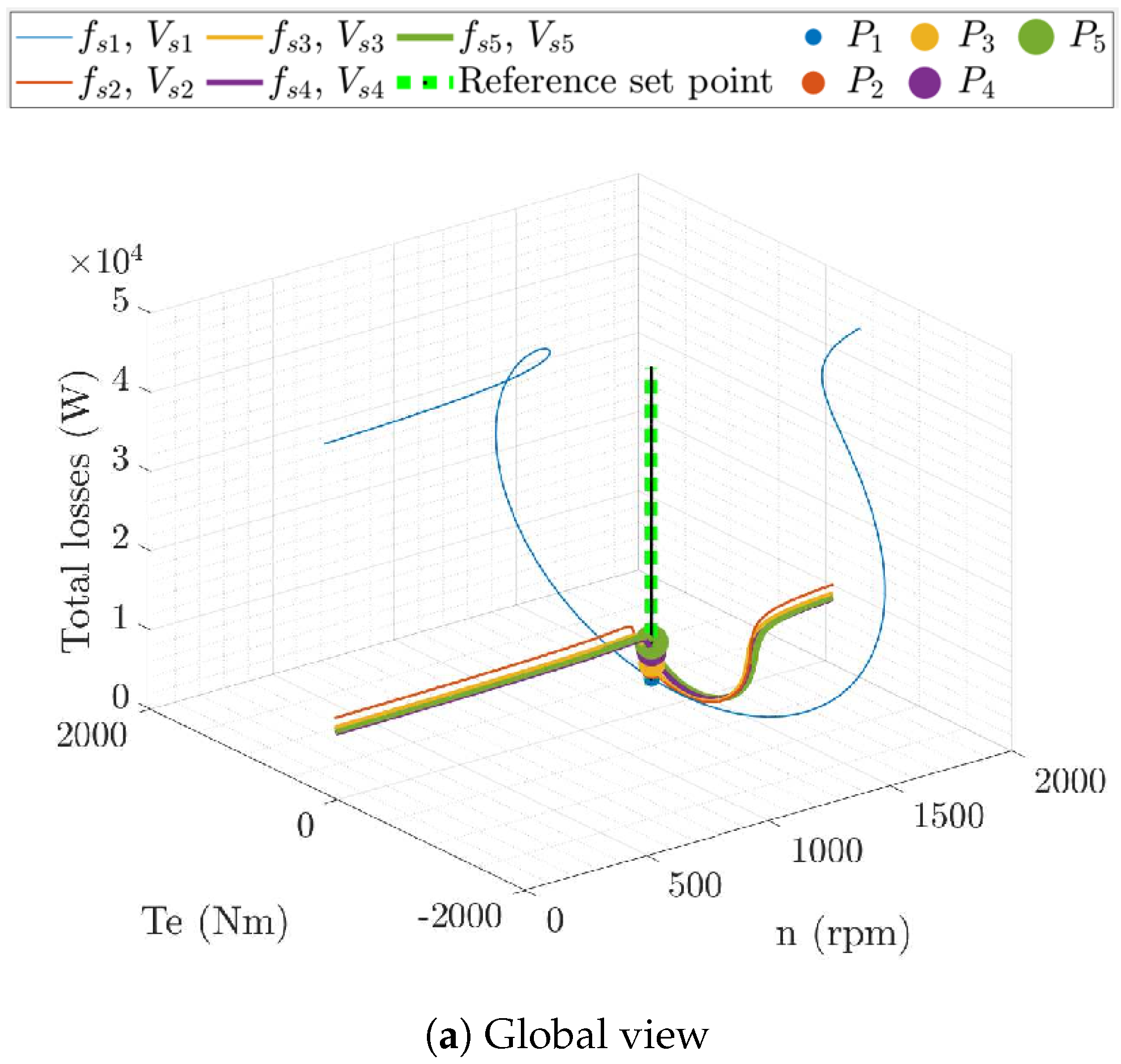
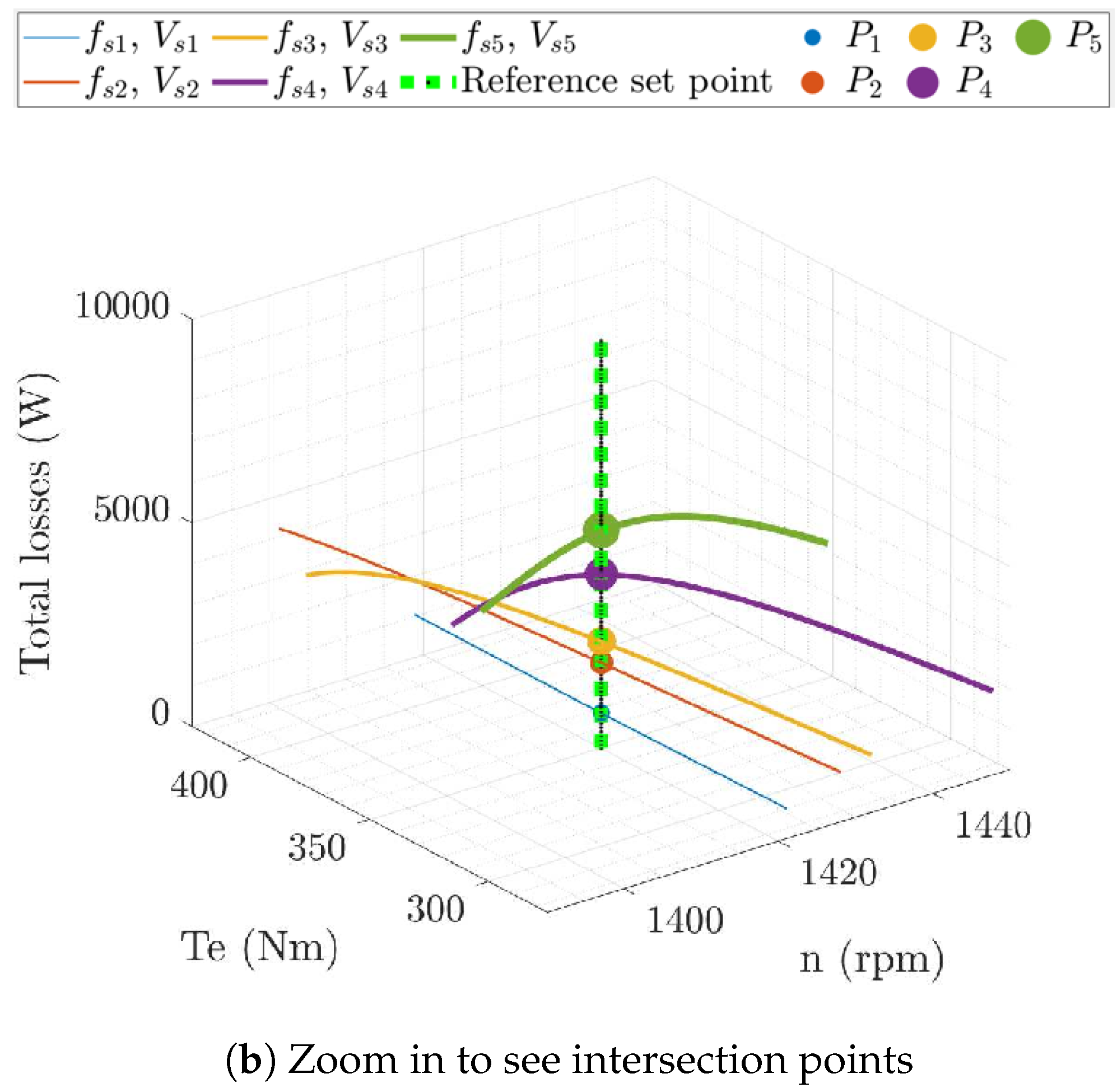
2.1.3. Total Loss Minimization for a Given Operating Point

Given the nature of the proposed control problem, there exists a specific reference set point characterized by a designated electromagnetic torque and mechanical speed at which the motor operates. At this reference set point, various fixed stator voltage values (both magnitude and frequency) are viable. The graphical representation in Figure 3 illustrates a discrete set of curves for different voltage and frequency for a specific reference point (torque and speed). To enhance clarity and efficiency, only curves with minimal slip ($s<$ 0.05) are included.

The same set of fixed stator voltage frequency and magnitude curves, along with their corresponding total loss values, are computed using Equation (18); these are depicted in Figure 4a. Upon considering the specific reference set point, it becomes evident that each curve intersects the reference set point (now depicted as a line) with a different total loss value, as illustrated in Figure 4b. In this figure, the various intersection points are marked as $P_1$, $P_2$, $P_3$, $P_4$, and $P_5$.

Similarly, the identical set of fixed stator voltage magnitude and frequency curves, incorporating the stator flux magnitude, is presented in Figure 5a. The stator flux magnitude values at the reference set point for each curve are clearly delineated in Figure 5b. Once again, the intersection points $P_1$, $P_2$, $P_3$, $P_4$, and $P_5$ are depicted.

The values for the stator flux magnitude and total loss for the intersection points ($P_1$, $P_2$, $P_3$, $P_4$, and $P_5$) in Figure 4b and Figure 5b are represented in Figure 6. A continuous curve representing the total losses as a function of the stator flux magnitude is obtained for the specific reference set point (torque and speed) by means of a spline regression [37].

The procedure described for a specific reference set point in Figure 3, Figure 4, Figure 5 and Figure 6 is repeated for various reference set points (torque and speed) that extend the entire operational range of the motor. This results in a series of regression curves that express total losses as a function of stator flux magnitude for different operating conditions.

For better visualization, a discrete subset of these curves is illustrated in Figure 7. Each curve in this set exhibits a minimum total loss point corresponding to a specific stator flux magnitude, denoted as ${\mathsf{\Psi }}_{s_{ref}}={\mathsf{\Psi }}_{s_{opt}}$ (referred to as the “optimum stator flux magnitude for total loss minimization”), which is also represented in the figure.

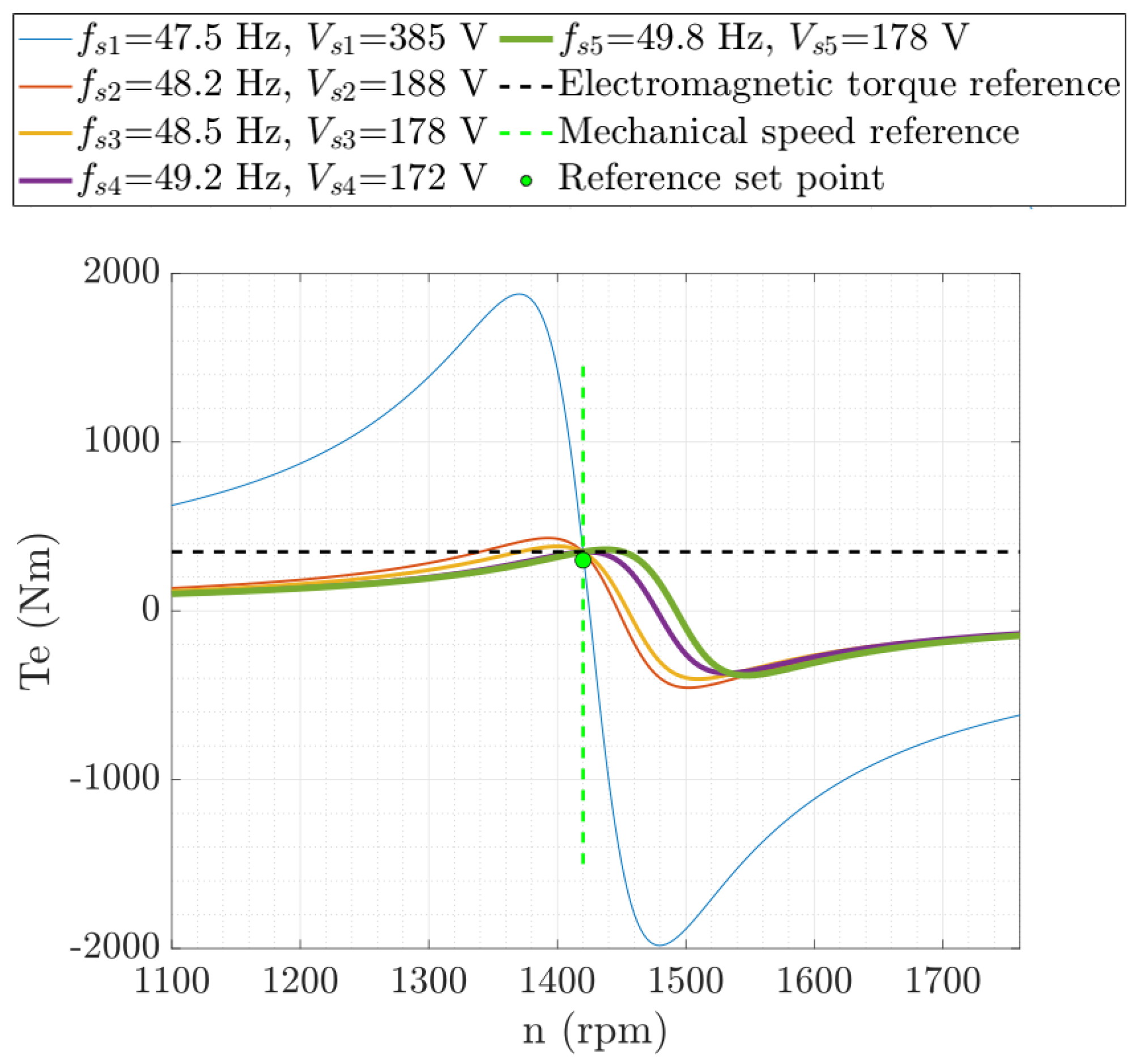
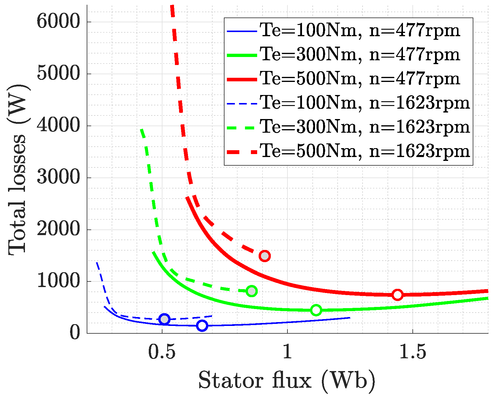
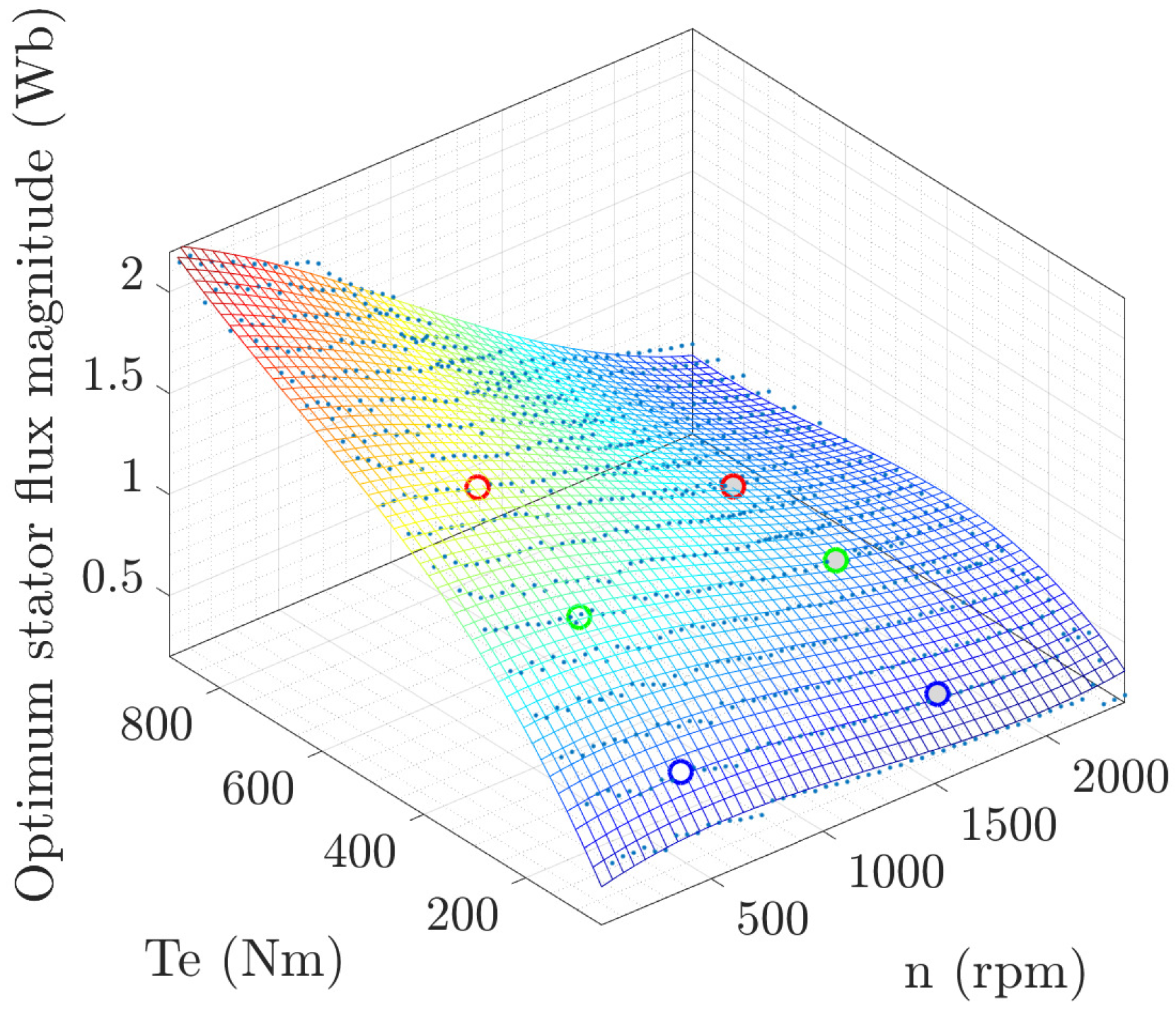
2.1.4. Optimum Stator Flux for a Given Rotor Speed and Electromagnetic Torque

The selected optimum stator flux magnitude value for loss minimization is represented as a function of the electromagnetic torque and mechanical speed across a wide set of discrete reference points, totaling nearly 1000 nodes and spanning the entire operational range of the motor. These discrete points, shown as small blue dots in Figure 8, include the example points depicted in Figure 7. A continuous third-order polynomial regression surface for optimum stator flux, which minimizes total losses as a function of mechanical speed and electromagnetic torque, is also represented. The resulting equation for the polynomial regression surface in Figure 8 and given by Equation (19) has a very low computational cost and is very easy to implement in terms of control. Consequently, this equation constitutes the core of the flux optimizer block introduced in the methodology section and depicted in Figure 1, where it is responsible for generating the total loss-minimizing stator flux reference ${\mathsf{\Psi }}_{s_{ref}}$. This equation provides a convenient way to generate the optimum reference stator flux value for given reference electromagnetic torque and mechanical speed values in the induction motor, thereby achieving total electric loss minimization.

$$\begin{array}{c}{\mathsf{\Psi }}_{s_{opt}}=p_{00}+p_{10}·n_{ref}+p_{01}·T_{e_{ref}}+p_{20}·n_{ref}^2\hfill \\ \hspace{1em}\hspace{1em}\hspace{1em}\hspace{1em}\hspace{1em}\hspace{1em}\hspace{1em}\hspace{1em}+p_{11}·n_{ref}·T_{e_{ref}}+p_{02}·T_{e_{ref}}^2+p_{30}·n_{ref}^3+\hfill \\ \hspace{1em}\hspace{1em}\hspace{1em}\hspace{1em}\hspace{1em}\hspace{1em}\hspace{1em}\hspace{1em}\hspace{1em}\hspace{1em}\hspace{1em}\hspace{1em}\hspace{1em} p_{21}·n_{ref}^2·T_{e_{ref}}+p_{12}·n_{ref}·T_{e_{ref}}^2+p_{03}·T_{e_{ref}}^3.\hfill \end{array}$$

(19)

Regression coefficients $p_{00}$ and $p_{10}$,...$p_{03}$ are numerical values obtained from the machine model parameters and limitations (i.e., working regions to be avoided, such as those exceeding stator current limitations). They are computed numerically following the loss-minimization procedure outlined in Section 2.1.3, prior to implementing the proposed MPC. Consequently, the computational cost of the numerical loss-minimization algorithm does not pose a setback in terms of online implementation, as the algorithm is executed only once before being implemented in the MPC strategy to determine the coefficients $p_{00}$, $p_{10}$,...$p_{03}$.

The loss-minimization algorithm is conveniently provided as a user-friendly Matlab function in [38]. This function yields the regression coefficients specified in Equation (19), based on the required parameters and limitations of the induction motor model, thus facilitating the implementation of any MPC. In Equation (20), the values of the parameters in Equation (19) are shown using the motor parameters indicated in

Table 2. Parameters for the used induction motor.

Parameter	Value
Pairs of poles (p)	2
Stator resistance ($R_s$)	0.0074 $\Omega$
Rotor resistance ($R_r$)	0.0084 $\Omega$
Magnetizing inductance ($L_m$)	12.8 mH
Stator leakage inductance ($L_{\sigma s}$)	0.385 mH
Rotor leakage inductance ($L_{\sigma r}$)	0.385 mH
Nominal power ($P_{nom}$)	100 kW
Maximum stator current ($I_{max}$)	600 A
DC link voltage ($V_{dc}$)	565 V
Nominal stator flux (${\mathsf{\Psi }}_{s_{nom}}$)	1.03 Wb
Nominal speed ($n_{nom}$)	1485 r/min

.

$$\begin{array}{ccc}\hfill \left[\begin{array}{c}{p}_{00}\\ p_{10}\\ p_{01}\\ p_{20}\\ p_{11}\end{array}\right]=\left[\begin{array}{c}0.1188\\ 6.6284·{10}^{-4}\\ 0.0061\\ -1.231·{10}^{-5}\\ -5.488·{10}^{-6}\end{array}\right]& \hfill & \hfill \left[\begin{array}{c}{p}_{02}\\ p_{30}\\ p_{21}\\ p_{12}\\ p_{03}\end{array}\right]=\left[\begin{array}{c}-1.018·{10}^{-5}\\ 3.320·{10}^{-8}\\ -1.260·{10}^{-9}\\ -2.990·{10}^{-9}\\ 7.688·{10}^{-9}\end{array}\right]\end{array}$$

(20)

The availability of this function is a key contribution of this paper, as it provides an optimal stator flux reference generator for any entity interested in deploying a lossminimizing model-based control for an induction motor. Using the function does not require a deep understanding of the loss-minimization algorithm, offering an advantage in terms of accessibility compared to other proposals for loss minimization. Unlike many optimization functions found in the literature, the proposed function is based on a comprehensive induction motor model without significant simplifications. Furthermore, it imposes no additional online computational burden, which helps preserve computational resources for other control elements. In fact, the proposed MPC strategy, combined with the precomputed flux reference for loss minimization, requires approximately 10–13k Floating Point Operations per Second (FLOPs), whereas implementing loss minimization online inside the MPC function would demand 30–35k FLOPs, significantly increasing real-time computational complexity.

The optimal stator flux reference generator is designed based on the steady-state operating points of the induction motor. To ensure smooth performance in highly dynamic applications, it is recommended to implement a gradual ramping mechanism for adjusting the reference values, preventing abrupt changes.

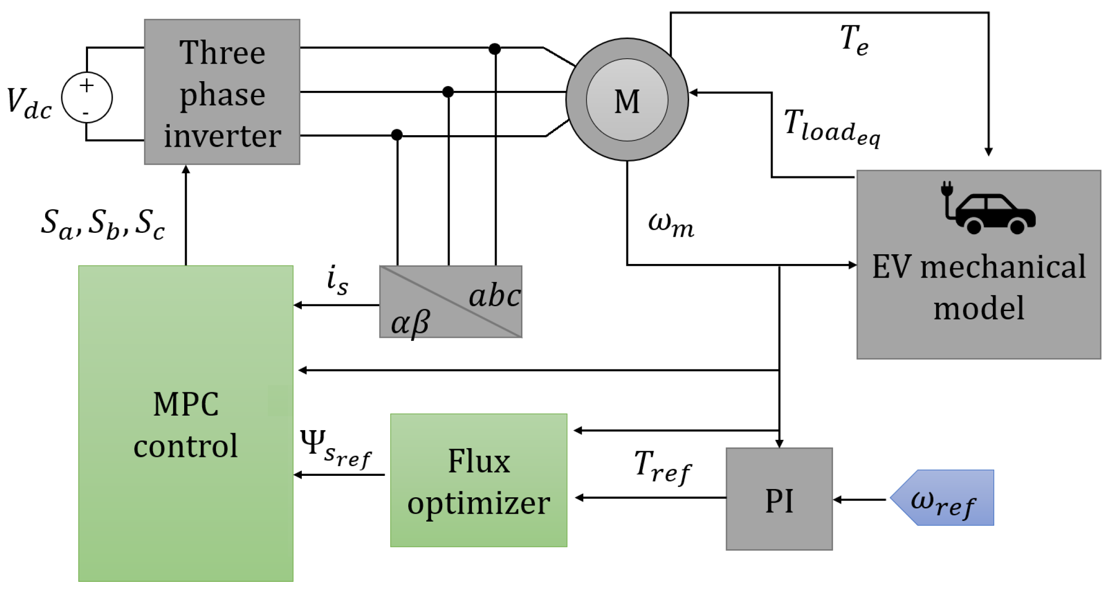
2.2. Model Predictive Control Strategy

The MPC strategy optimizes the output voltage of the inverter based on a cost function that considers the absolute normalized error of the reference electromagnetic torque and the stator flux, giving equal importance to both terms. The cost function is shown in Equation (21):

$$g_{cf}=\left\{\begin{array}{cc}\sum _{i=1}^3{\lambda }_{\phi }·{\displaystyle \frac{|\left|\overline{{\phi }_{s_{k+i}}}\right|-{\phi }_{s_{\mathrm{ref}}}|}{{\phi }_{s_{\mathrm{nom}}}}}+{\lambda }_T·{\displaystyle \frac{|T_{e_{k+i}}-T_{e_{\mathrm{ref}}}|}{T_{e_{\mathrm{nom}}}}},\hfill & \mathrm{if}\left|\overline{i_s}\right|\le I_{\lim },\hfill \\ \infty ,\hfill & \mathrm{otherwise}.\hfill \end{array}\right.$$

(21)

Here, ${\lambda }_{\phi }$ and ${\lambda }_T$ are the weighting factors for the stator flux and torque, respectively. Equal importance is given to both terms by setting ${\lambda }_{\phi }={\lambda }_T=1$. $I_{\lim }$ represents the current limit of the inverter for safe operation. $\overline{{\phi }_{s_{k+i}}}$ is the predicted stator flux magnitude at prediction step $k+i$, where i aligns with the modulation strategy described in subsequent sections. $T_{e_{k+i}}$ is the predicted torque at prediction step $k+i$.

The optimized reference values for stator flux magnitude and torque are ${\phi }_{s_{\mathrm{ref}}}$ and $T_{e_{\mathrm{ref}}}$, respectively. Finally, ${\phi }_{s_{\mathrm{nom}}}$ and $T_{e_{\mathrm{nom}}}$ denote the nominal values of the stator flux magnitude and the torque of the machine.

2.2.1. Induction Motor Model Discretization

The induction motor model described in Equations (9) and (10) is discretized using the forward Euler method [39]. The values of the space vector variables in $\mathbf{s}$ at time instant $k+1$ are predicted based on the measured or estimated values of the variables in $\mathbf{s}$ and $\mathbf{v}$ at time instant k, as shown in Equation (22):

$${\mathbf{s}}_{k+1}={\mathbf{A}}_v{\mathbf{v}}_k-{\mathbf{A}}_s{\mathbf{s}}_k,$$

(22)

where ${\mathbf{A}}_v$ and ${\mathbf{A}}_s$ are the discretization matrices.

If time instants $k+1$ and k are separated by a sample time $T_s$, the matrices ${\mathbf{A}}_v$ and ${\mathbf{A}}_s$ are computed as follows:

$$\begin{array}{cc}\hfill {\mathbf{A}}_v& ={(\mathbf{C}+\mathbf{D}·\mathbf{E})}^{-1}·T_s,\hfill \end{array}$$

(23)

$$\begin{array}{cc}\hfill {\mathbf{A}}_s& =T_s·{(\mathbf{C}+\mathbf{D}·\mathbf{E})}^{-1}(\mathbf{A}+\mathbf{B}·\mathbf{E})-\mathbf{I},\hfill \end{array}$$

(24)

where the values of the matrices $\mathbf{A}$, $\mathbf{B}$, $\mathbf{C}$, $\mathbf{D}$, and $\mathbf{E}$ are specified in Equations (12) and (13).

2.2.2. MPC Using Iron Loss Model

The compact matrix form of the induction motor electric model discretization method in Equation (22) facilitates the implementation of the MPC. Moreover, it allows perfect coherency of MPC with the electric model for the motor. The MPC model can consider iron losses when required, consequently making variable predictions more accurate. The coherency provided through the use of the same induction motor model for the lossminimization algorithm, motor implementation, and MPC implementation differs from other approaches often seen in the literature [24,26].

2.2.3. $V_i,V_0,V_i$ Control Vector Strategy

The inputs for the electrical system controlled by the MPC are the states of the inverter gates. For a two-level, three-phase inverter, there are a total of eight combinations. These inverter gate states are directly related to the seven options $V_0$–$V_7$ for the stator voltage of the induction motor [40]. The choice of a certain input vector will affect the values of the induction motor variables controlled by the MPC (electromagnetic torque and stator flux). In this paper, two different input vector strategies are considered, and they are described below:

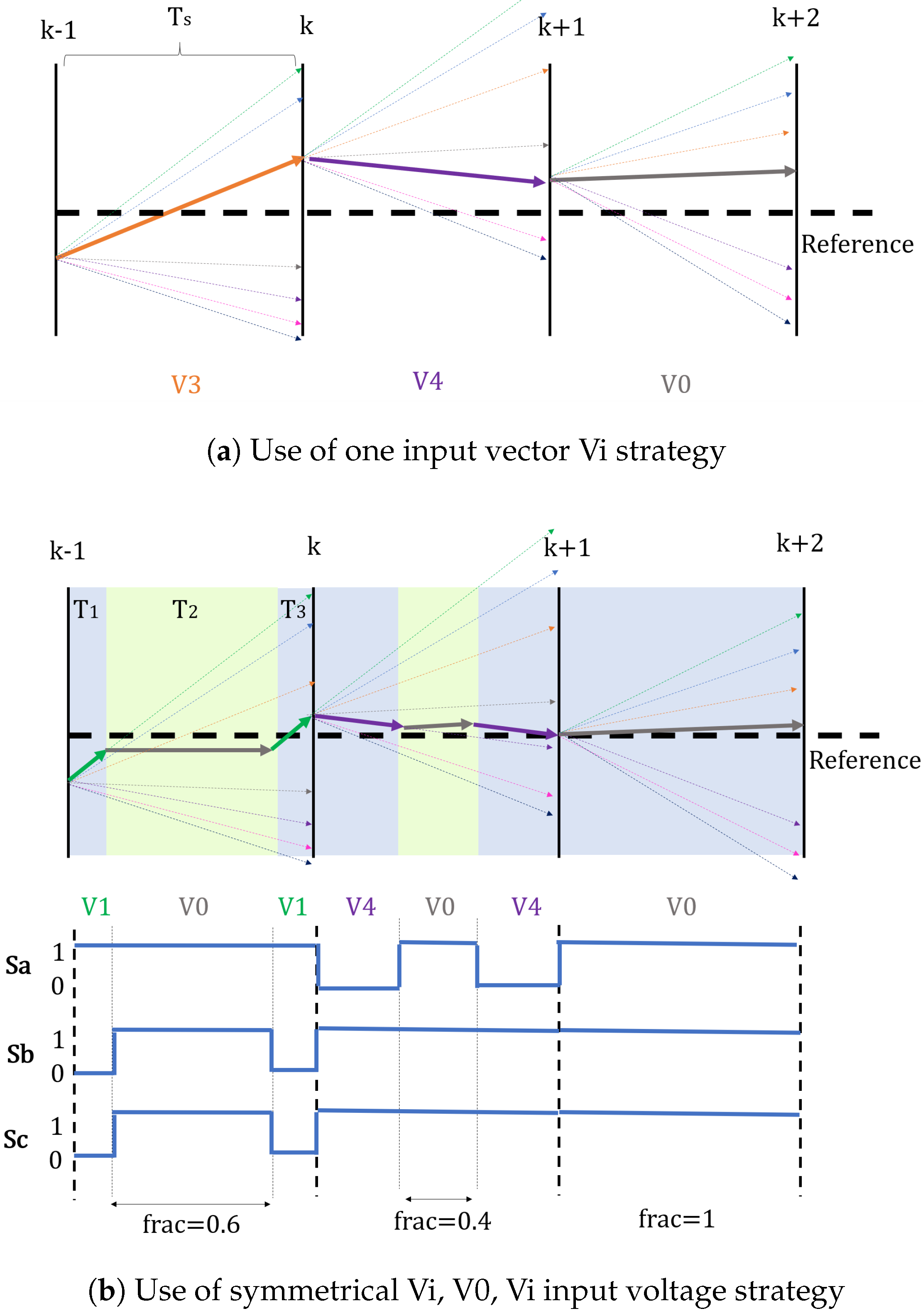
• $V_i$ Strategy: This input strategy considers the effect of selecting each input voltage vector ($V_0$–$V_7$) on the output variables (electromagnetic torque and stator flux) and on maintaining the selected vector during the sample time $T_s$. The input voltage is chosen based on the vector that provides a value closest to the reference output variable. This process is graphically illustrated for the stator flux in Figure 9a.
• $V_i,V_0,V_i$ Strategy: This strategy involves commanding a three-voltage symmetric vector sequence ($V_i,V_0,V_i$) instead of a single $V_i$. Consequently, the controller not only selects among the seven possible discrete voltage options for $V_i$ but also determines the proportion of the sample time $T_s$ during which the vectors $V_i$ and $V_0$ are applied. This is achieved using a discrete variable called frac.
  The total sample time is divided into three distinct intervals: $T_1$, $T_2$, and $T_3$, defined based on the variable frac, as shown in Equations (25) and (26):

  $$\begin{array}{cc}\hfill T_1& =T_3={\displaystyle \frac{1-\mathrm{frac}}{2}}{T}_s,\hfill \end{array}$$

  (25)

  $$\begin{array}{cc}\hfill T_2& =\mathrm{frac}·T_s.\hfill \end{array}$$

  (26)
  After performing a cost–reward analysis in terms of computational efficiency, the possible discrete values for $frac$ are set to 0, 0.2, 0.4, 0.6, 0.8, and 1. The effect of the selected input voltage combination on the output variables is considered at three points during a sample time $T_s$ instead of one point. The combination of input vectors and the values of the variable $frac$ selected at each $T_s$ provide values for the output variable closest to the reference. This process is performed by considering the predicted values for the output variable during $T_s$ ($T_1$, $T_2$, and $T_3$) instead of just at the end of $T_s$. This process is graphically explained for the stator flux in Figure 9b. A symmetrical $V_i,V_0,V_i$ strategy allows three different voltage vectors to be applied during a time sample $T_s$ with just one inverter leg command per $T_s$ by commanding an appropriate duty cycle (see the inverter leg commands in Figure 9b).

The $V_i,V_0,V_i$ strategy provides more precise control of output variables because more input and output combinations are considered. In addition, it provides a lower ripple for the controlled variables relative to their reference values, as the output variables are predicted throughout $T_s$ and not only at the end of $T_s$. The ripple reduction is graphically depicted in Figure 9, showing the effect of using both strategies during three sample times when following a given stator flux reference. This improvement is achieved at the expense of a slight increase in computational cost. However, the computational cost of this strategy is not disproportionate with respect to the $V_i$ strategy, nor is it impractical in terms of implementation given the computational speed of today’s microcontrollers [41]. However, if computational speed is not a limiting factor, one may wonder if there is an advantage to using a $V_i,V_0,V_i$ vector strategy as opposed to a $V_i,V_j,V_i$ or $V_i,V_j,V_k$ vector strategy. The main advantage is that a symmetric $V_i,V_0,V_i$ sequence is the only one that allows three different voltage vectors to be applied for a time sample $T_s$ with only one inverter leg command per $T_s$. This is a clear advantage in terms of control precision. This also results in a lower switching frequency for inverter legs compared to other three-vector voltage strategies. Minimizing the inverter leg switching frequency is also crucial in terms of reducing inverter losses [16,17,42].

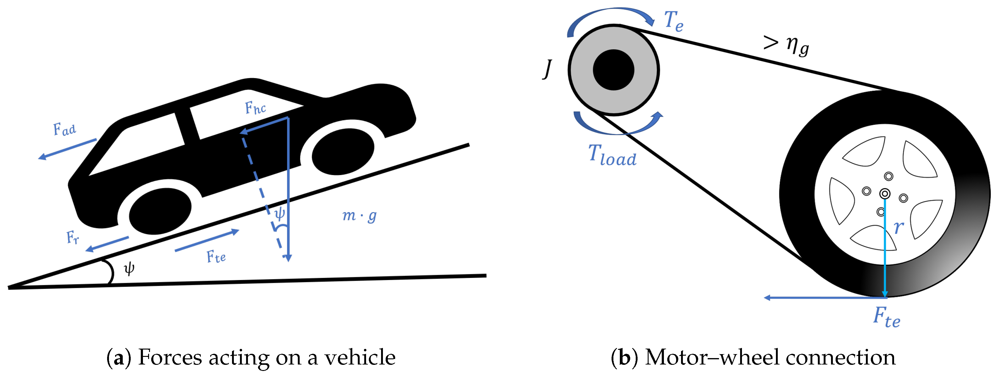
2.2.4. Mechanical Model of the Electric Vehicle

The mechanical model for the electric vehicle is developed according to wellestablished literature on the topic [43]. Figure 10a and Equations (27)–(31) describe the linear mechanical forces acting on the electric vehicle. Figure 10b and Equations (32)–(34) represent the rotational dynamics in the induction motor as a result of these mechanical forces.

$$\begin{array}{cc}\hfill F_{te}& =F_{ad}+F_{hc}+F_r-m·a,\hfill \end{array}$$

(27)

$$\begin{array}{cc}\hfill a& ={\displaystyle \frac{d\omega }{dt}}·{\displaystyle \frac{r}{G}},\hfill \end{array}$$

(28)

$$\begin{array}{cc}\hfill F_{ad}& ={\displaystyle \frac{1}{2}}\rho ·A·C_d·v^2,\hfill \end{array}$$

(29)

$$\begin{array}{cc}\hfill F_{hc}& =m·g·sin\psi ,\hfill \end{array}$$

(30)

$$\begin{array}{cc}\hfill F_r& =m·g·{\mu }_r·cos\psi ,\hfill \end{array}$$

(31)

where $F_{te}$ is the tractive effort, $F_{ad}$ is the aerodynamic drag force, $F_{hc}$ is the hill climbing force, $F_r$ is the rolling resistance force, m is the vehicle mass, a is the vehicle acceleration, $\rho$ is the air density, A is the frontal area of the vehicle, $C_d$ is the drag coefficient, v is the vehicle linear velocity, g is the gravitational acceleration, $\psi$ is the road slope angle, and ${\mu }_r$ is the rolling resistance coefficient.

$$\begin{array}{cc}\hfill T_e-T_{{\mathrm{load}}_{\mathrm{eq}}}& =J_{\mathrm{eq}}{\displaystyle \frac{d\omega }{dt}},\hfill \end{array}$$

(32)

$$\begin{array}{cc}\hfill J_{\mathrm{eq}}& =J+m{\displaystyle \frac{r^2}{G^2{\eta }_g}},\hfill \end{array}$$

(33)

$$\begin{array}{cc}\hfill T_{{\mathrm{load}}_{\mathrm{eq}}}& =F_{te}·{\displaystyle \frac{r}{G·{\eta }_g}},\hfill \end{array}$$

(34)

where $T_e$ is the electromagnetic torque, $T_{{\mathrm{load}}_{\mathrm{eq}}}$ is the equivalent load torque, $J_{\mathrm{eq}}$ is the equivalent moment of inertia, J is the motor inertia, r is the wheel radius, G is the gearbox ratio, and ${\eta }_g$ is the gearbox efficiency.

3. Results

Dynamic simulation case studies are performed to assess the performance of the MPC proposed in this paper in both EV and non-EV environments (induction motor only). Its performance will be compared to the classical direct-torque MPC used for induction motors in [40]. First, a series of speed and torque dynamic response tests are conducted in the Matlab/Simulink 2024b environment using only the induction motor to test the proposed control performance. The proposed control is then validated for EV applications using the ECE-15 and WLTP-Urban driving cycles. In addition, its robustness to variations in motor parameters is examined, considering changes in stator resistance and magnetizing inductance to assess performance under real-world uncertainties.

3.1. Induction Motor Parameters

All simulations and case studies are conducted using a four-pole induction motor with the parameters in Table 2.

This motor model accounts for iron losses by representing the magnetizing branch as a series combination of a frequency-dependent iron loss resistance, $R_{fe,s}$, and a magnetizing inductance, $L_{m,s}$. The series resistance is given by

$$R_{fe,s}=\left\{\begin{array}{cc}1.7967\times {10}^{-3}+17.949\times {10}^{-6}{\omega }_s+2.8891\times {10}^{-8}{\omega }_s^2,\hfill & \mathrm{if}f\le 50\mathrm{Hz},\hfill \\ 25.542\times {10}^{-3}-{\displaystyle \frac{4.821}{{\omega }_s}},\hfill & \mathrm{if}f>50\mathrm{Hz},\hfill \end{array}\right.$$

(35)

where $R_{fe,s}$ is the series iron loss resistance, ${\omega }_s$ is the stator angular frequency, and f is the supply frequency. Equation (35) is derived via regression from the iron loss resistance data reported in [35,44] for a 4 kW motor in a parallel branch configuration. The original data were used to formulate an expression for $R_{fe,s}$ in the series configuration with a magnetizing inductance $L_{m,s}$, and the values were subsequently scaled to match the dimensions and rated power of the 100 kW motor analyzed in this study.

It is noted that when computing $L_{m,s}$ using the regression values, the variation with ${\omega }_s$ is minimal. Therefore, for the purposes of this case study, $L_{m,s}$ is assumed to be constant and equal to $L_m$. While this formulation is tailored to the present motor, the control framework is flexible and can accommodate alternative $R_{fe}$ models, ensuring applicability to diverse motor designs and operating conditions. Ultimately, the most accurate representation of iron losses would be obtained through a parametrization based on experimental measurements of the specific machine under control—a task that is beyond the scope of this paper.

3.2. Control Objectives

The three main objectives of the MPC proposed in this research are the following.

• The minimization of total electric energy losses during dynamic simulation periods, steady-state operation, and EV driving cycles. The total electric energy losses will be evaluated using Equation (18).
• The minimization of the electromagnetic torque ripple of the induction machine to reduce the mechanical fatigue of the shaft and the mechanical resonance vibration [45,46,47]. This will be evaluated by considering the root-mean-square error (RMSE) between the measured electromagnetic torque of the induction machine and the reference electromagnetic torque generated by the PI controller.
• The ability to follow a given mechanical speed reference with precision during both transient and steady-state operation. This will be evaluated by considering the RMSE between the measured mechanical speed of the induction motor and the reference speed.

To quantify the improvements achieved by the proposed control compared to the classic control, the percentage reduction in each performance metric is calculated as follows:

$$\mathrm{Reduction} (\%)=\left({\displaystyle \frac{\mathrm{Classic}\mathrm{Control}\mathrm{Value}-\mathrm{Proposed}\mathrm{Control}\mathrm{Value}}{\mathrm{Classic}\mathrm{Control}\mathrm{Value}}}\right)\times 100$$

(36)

In Equation (36), Classic Control Value represents the performance metric value under the classic control approach, while Proposed Control Value represents the corresponding value under the proposed MPC scheme. This formula provides a clear measure of the relative improvement offered by the proposed control, expressed as a percentage reduction relative to the baseline performance of the classic control.

3.3. Speed and Load Torque Dynamic Response Tests

A dynamic simulation is conducted to evaluate the performance of the proposed MPC control strategy under varying load and speed reference conditions. The proposed control has three innovative features that do not exist in the classical direct torque MPC most commonly used in the literature [8,25,26]. These features include a torque ripple reduction strategy (Section 2.2.3), incorporating the iron loss model into MPC design, and employing a flux reference function for electric loss minimization (Section 2.1.4) instead of a nominal flux reference function for electric loss minimization described in Section 2.1.4 instead of a nominal flux reference (with flux weakening being accounted for at higher speeds [48,49]).

Figure 11 illustrates the dynamic response of both the classic and proposed MPC control during a series of relevant dynamic events designed to evaluate their performance. These events include the following:

• Acceleration and deceleration speed ramps: Reference speed ramps with dynamics 10 times faster than typical urban driving conditions. These scenarios are tested under both loaded and unloaded conditions to assess control performance across varying operational states.
• Operation above nominal speed: Reference speeds exceeding the motor’s nominal speed, forcing a transition from the constant torque region to the constant power region. In this region, both control strategies apply flux weakening to protect the stator winding insulation from breakdown.
• Variable loading torque: Dynamic changes in loading torque are introduced to evaluate the ability of each control strategy to respond effectively to varying mechanical loads.

The numerical performance metrics for the control objectives set in Section 3.2 for the classic and proposed control are summarized in

Table 3. Reduction in error performance metrics: proposed control compared to classic control for the speed and torque dynamic response test.

Metric	Reduction (%)
RMSE Speed Error (Measured vs. Reference Values)	8.06%
RMSE Torque Error (Measured vs. Reference Values)	85.39%
Total Electric Losses	2.84%
Current THD	37.97%

. It also contains the percentage reduction in Total Harmonic Distortion (THD) of the currents during the first steady-state segment of the dynamic test.

One may observe from Figure 11e,f that both controls accurately follow the reference speed during transient and steady-state operation. This performance can be attributed to the well-known ability of the MPC to handle dynamic systems.

The proposed control visibly reduces electromagnetic torque ripple, resulting in smoother motor operation compared to the classic MPC. As a consequence, the THD in the measured currents is also significantly lower.

By analyzing Figure 11g,h, one can observe how, after the startup phase, the proposed MPC control consistently adjusts the stator flux reference value to minimize the motor’s total electric losses specifically for its operation point both in the constant torque and constant power region. At no point does the classical MPC control optimize the flux to minimize losses; it only weakens the flux when the motor operates in the constant power region. This translates to lower measured total electric losses when the proposed control is used. While the loss-minimizing feature performs better during steady-state operation than transients, it remains effective in dynamic tests combining transient and steady-state regions, as shown in this section.

3.4. Robustness of the Proposed Control Strategy to Motor Parameter Variations

Although numerous studies in the literature [50,51,52] have demonstrated a strong alignment between experimental and simulation results when an accurate electrical model of the machine is used, real-world factors such as aging, thermal effects [53], manufacturing tolerances [54], and magnetic saturation [55] can cause deviations in motor parameters. These variations may impact control performance, making robustness a crucial consideration.

To assess the dynamic robustness of the proposed MPC strategy, key motor parameters were intentionally perturbed, and the system’s response was analyzed under the following conditions:

• The stator resistance ($R_s$) was varied from $-20\%$ to $+50\%$ to account for manufacturing tolerances, aging, and temperature-dependent changes.
• The magnetizing inductance ($L_m$) was varied by $\pm 20\%$ to simulate magnetic saturation and manufacturing tolerances.

Table 4. Robustness analysis results. The baseline cases correspond to the nominal parameters for the classic and proposed control strategies.

Parameter Variation	RMSE	RMSE
	Torque Ripple (%)	Speed Tracking (%)
Baseline (Classic)	$1.5$	$2.65\times {10}^{-3}$
Baseline (Proposed)	$0.22$	$2.43\times {10}^{-3}$
+50% $R_s$	$0.52$	$2.43\times {10}^{-3}$
−20% $R_s$	$0.86$	$2.5\times {10}^{-3}$
+20% $L_m$	$0.3$	$2.43\times {10}^{-3}$
−20% $L_m$	$0.36$	$2.44\times {10}^{-3}$

summarizes the impact of these parameter variations on key performance metrics, including speed RMSE and torque ripple RMSE, during the dynamic tests outlined in Section 3.3. For reference, the table also includes baseline results for both the classic and proposed control strategies under nominal (unchanged) parameter conditions.

The proposed control strategy demonstrates strong robustness in speed tracking, maintaining low RMSE values even when motor parameters are varied due to aging, temperature fluctuations, and magnetic saturation. The results indicate high robustness against variations in magnetizing inductance, suggesting that the control effectively mitigates the effects of magnetic saturation. In contrast, while the control also exhibits acceptable robustness to stator resistance variations, it is more sensitive to decreases in resistance (e.g., due to lower temperatures) than to increases (e.g., caused by heating or aging). This suggests that parameter estimation should ideally be performed under cooler operating conditions to ensure optimal performance across a wide range of scenarios. Despite these variations, the proposed control consistently outperforms the classic control, confirming its superior adaptability and effectiveness under real-world parameter uncertainties.

To evaluate the robustness of the proposed loss-minimizing stator flux reference function, the total electrical losses during steady-state operation were analyzed at both medium-load and low-load conditions under varying motor parameters. Full-load conditions were excluded, as the flux optimizer selects the nominal flux under these conditions, making loss minimization negligible. The results, summarized in

Table 5. Robustness analysis of the loss-minimizing function. The table presents the total electrical losses as a percentage of the baseline classic MPC losses.

Parameter Variation	Medium Load (% of Baseline)		Low Load (% of Baseline)
	Classic MPC	Proposed MPC	Classic MPC	Proposed MPC
Baseline	100	$73.6$	100	$38.9$
+50% $R_s$	$132.4$	$121.3$	$133.7$	$35.7$
−20% $R_s$	$89.3$	$82.4$	$89.9$	$40.8$
+20% $L_m$	$83.4$	80	$78.7$	24
−20% $L_m$	$129.0$	114	$138.7$	$55.7$

, are normalized with respect to the total losses in the classic MPC baseline case to facilitate a direct comparison. The table presents the losses as a percentage of the baseline value, where values below 100% indicate improved efficiency. The comparison includes the classic MPC control without loss minimization and the proposed control incorporating the loss-minimizing function. The results demonstrate the effectiveness of the proposed strategy in minimizing losses across different motor parameter variations.

3.5. EV Application Using the ECE-15 and WLTP-Urban Driving Cycles

In order to validate the proposed MPC control strategy for the EV application, both the ECE-15 and WLTP-Urban drive cycles were used as inputs for the motor, employing the mechanical model explained in Section 2.2.4. The ECE-15 drive cycle is an urban driving cycle designed to represent city driving conditions, specifically focusing on the emissions and fuel consumption of light-duty vehicles. The specific operating points for this driving cycle are detailed in [43]. This driving test is widely used due to its acceptance in the literature, established validity, and reliability. Additionally, it facilitates direct comparisons with prior studies, ensuring methodological consistency and robust benchmarking of performance outcomes.

However, in regulatory and industry standards, the WLTP-Urban cycle [56] has replaced ECE-15 as the standard procedure for evaluating EV performance, as it more accurately represents the dynamic conditions of urban driving. The first segment of the WLTP (WLTP-Urban) is specifically designed to reflect modern urban traffic patterns, including frequent acceleration and deceleration events. This test provides a more representative assessment of the efficiency and control performance of an EV in city environments. By incorporating both tests, this study ensures a comprehensive evaluation of the proposed control strategy for EV applications, using the historical acceptance of ECE-15 and the improved relevance of WLTP-Urban in the real world.

The numerical parameters for the EV mechanical model used in these tests are listed in

Table 6. Parameters used for the electric vehicle model.

Parameter	Value
Mass, m	1000 kg
Gearbox ratio, G	3.2
Radius of the wheel, r	0.26 m
Frontal area of the vehicle, A	2.4 m2
Drag coefficient, $C_d$	0.3
Air density, $\rho$	1.223 kg/m3
Efficiency of the gearbox, ${\eta }_g$	0.8
Acceleration due to gravity, g	9.81 m/s2
Road slope, $\psi$	0º
Coefficient of rolling resistance, ${\mu }_r$	0.01

.

In Figure 12, the performance of the electric motor is depicted using the proposed MPC control for both the ECE-15 and WLTP-Urban driving cycles. As shown in Figure 12a,b, the electromagnetic torque of the motor, $T_e$, exhibits minimal ripple, consistent with the discussion in previous sections. The accelerating torque closely matches the expected values required to achieve the speed profile shown in Figure 12c,d. Notably, throughout the cycle, the electric motor speed closely follows the reference speed.

In Figure 12e,f, the magnitude of the stator flux and its reference value, as provided by the proposed MPC control, are shown. It can be observed that the flux values are continuously optimized after startup (where nominal flux is used) to minimize total electric losses.

Table 7. Reduction in error performance metrics: proposed control compared to classic control for ECE-15 and WLTP-Urban driving tests.

Metric	Reduction (%)
	ECE-15	WLTP-Urban
RMSE Torque Error (Measured vs. Reference)	93.23	93.55
Total Electric Losses	51.57	49.11

presents the improvement in performance metrics for the proposed vs. the classic MPC control during the ECE-15 and WLTP-Urban driving tests. For a more detailed statistical evaluation of control performance, including RMSE, MAE, and confidence intervals across all test scenarios, please refer to Appendix A. The proposed control significantly improves the torque ripple, which has a beneficial effect on current harmonics. The reduction in torque ripple achieved by the proposed MPC compared to the classical MPC can lead to a 20% increase in the lifespan of drivetrain mechanical components (such as the gearbox) [57]. The most notable improvement is in total electric losses (copper and iron), with the proposed control reducing total electric losses by 51.57% during the ECE-15 test and by 49.11% in the more dynamic WLTP-Urban test compared to the classical MPC. This highlights the suitability of the proposed control for EV applications, particularly in urban driving scenarios characterized by a mix of steady-state and transient operating conditions.

4. Conclusions

This work has introduced a novel optimization framework for induction motors in EV applications, distinguished by its integrated iron-loss modeling within the predictive control scheme, its offloaded polynomial-based approach to flux optimization, and its symmetrical voltage-vector strategy for torque ripple reduction. By unifying loss minimization and torque regulation in a coherent structure, the proposed method substantially reduces total electrical losses across typical operating points and achieves smoother torque profiles in low- and medium-speed regions. The resulting control strategy thus offers a practical, computationally tractable solution for next-generation electric drivetrains, as validated in both the ECE-15 and WLTP-Urban cycles.

The use of a $V_i,V_0,V_i$ inverter control strategy instead of the $V_i$ strategy for an induction motor MPC, combined with the incorporation of the iron loss model in the MPC design, has been shown to reduce torque ripple by 85% in the proposed dynamic tests. The proposed inverter switching strategy entails a higher computational demand for the MPC; however, this demand is not disproportionate compared to the classical strategy, nor is it impractical given the computational speed of today’s microcontrollers.

Replacing the nominal flux reference (which only accounts for flux weakening at higher speeds) with the proposed loss-minimizing stator flux reference significantly reduces total electrical losses. Although the loss-minimizing feature is primarily designed for steady-state operation, it remains effective in dynamic tests that involve both transient and steady-state conditions. The use of the proposed loss-minimizing flux reference incurs no additional computational cost during online control (already stressed by the MPC strategy itself) and also offers remarkable flexibility, as it can be tailored to any given induction motor parameters. Additionally, the proposed control strategy is highly adaptable, as the iron loss model and loss-minimizing flux reference can be tailored to different motor parameters or replaced with alternative formulations, ensuring broad applicability across various induction motor designs and operating conditions. Furthermore, its straightforward implementation and availability as an open-access resource in [38] make it highly accessible and practical for a wide range of applications.

The proposed control is particularly suitable for urban EV applications of all sizes, although it is not limited to them. During the two proposed driving cycles, the system closely follows the reference speed. In terms of energy efficiency, the total losses during an urban driving cycle are reduced by up to 49% when the proposed control is used. The reduction in torque ripple is also very significant, minimizing the shaft’s mechanical fatigue and mechanical resonance vibration when compared to the classical MPC, which can lead to a 20% increase in the lifespan of drivetrain mechanical components.

References

1. Moorkens, I.; Tomescu, M.; Das, A.; Emele, L.; Meinke-Hubeny, F.; Nissen, C. Renewable Energy in Europe—2018 Recent Growth and Knock-On Effects; Technical Report; European Environment Agency: Copenhagen, Denmark, 2018. [Google Scholar] [CrossRef]
2. Islam, M.S.; Mithulananthan, N.; Lee, K.Y. Development of impact indices for performing charging of a large EV population. IEEE Trans. Veh. Technol. 2017, 67, 866–880. [Google Scholar] [CrossRef]
3. Yi, P.; Zhu, T.; Jiang, B.; Jin, R.; Wang, B. Deploying energy routers in an energy internet based on electric vehicles. IEEE Trans. Veh. Technol. 2016, 65, 4714–4725. [Google Scholar] [CrossRef]
4. Bulut, M.S.; Ordu, M.; Der, O.; Basar, G. Sustainable Thermoplastic Material Selection for Hybrid Vehicle Battery Packs in the Automotive Industry: A Comparative Multi-Criteria Decision-Making Approach. Polymers 2024, 16, 2768. [Google Scholar] [CrossRef] [PubMed]
5. Cai, W.; Wu, X.; Zhou, M.; Liang, Y.; Wang, Y. Review and development of electric motor systems and electric powertrains for new energy vehicles. Automot. Innov. 2021, 4, 3–22. [Google Scholar] [CrossRef]
6. Lemmens, J.; Vanassche, P.; Driesen, J. Optimal Control of Traction Motor Drives Under Electrothermal Constraints. IEEE J. Emerg. Sel. Top. Power Electron. 2014, 2, 249–263. [Google Scholar] [CrossRef]
7. Kouro, S.; Cortes, P.; Vargas, R.; Ammann, U.; Rodriguez, J. Model Predictive Control—A Simple and Powerful Method to Control Power Converters. IEEE Trans. Ind. Electron. 2009, 56, 1826–1838. [Google Scholar] [CrossRef]
8. Rodriguez, J.; Cortes, P. Predictive Control of Power Converters and Electrical Drives; John Wiley & Sons: Hoboken, NJ, USA, 2012; Volume 40. [Google Scholar]
9. Wróbel, K.; Serkies, P.; Szabat, K. Model Predictive Base Direct Speed Control of Induction Motor Drive—Continuous and Finite Set Approaches. Energies 2020, 13, 1193. [Google Scholar] [CrossRef]
10. Wang, F.; Zhang, Z.; Mei, X.; Rodríguez, J.; Kennel, R. Advanced Control Strategies of Induction Machine: Field Oriented Control, Direct Torque Control and Model Predictive Control. Energies 2018, 11, 120. [Google Scholar] [CrossRef]
11. Zhang, Y.; Xia, B.; Yang, H.; Rodriguez, J. Overview of model predictive control for induction motor drives. Chin. J. Electr. Eng. 2016, 2, 62–76. [Google Scholar]
12. Hosseinzadeh, M.A.; Sarbanzadeh, M.; Sarebanzadeh, E.; Rivera, M.; Muñoz, J. Predictive Control in Power Converter Applications: Challenge and Trends. In Proceedings of the 2018 IEEE International Conference on Automation/XXIII Congress of the Chilean Association of Automatic Control (ICA-ACCA), Concepcion, Chil, 17–19 October 2018; pp. 1–6. [Google Scholar] [CrossRef]
13. Zhang, Y.; Yang, H. Generalized two-vector-based model-predictive torque control of induction motor drives. IEEE Trans. Power Electron. 2014, 30, 3818–3829. [Google Scholar] [CrossRef]
14. McInerney, I.; Constantinides, G.A.; Kerrigan, E.C. A survey of the implementation of linear model predictive control on fpgas. IFAC-PapersOnLine 2018, 51, 381–387. [Google Scholar] [CrossRef]
15. Geyer, T.; Papafotiou, G.; Morari, M. Model predictive direct torque control—Part I: Concept, algorithm, and analysis. IEEE Trans. Ind. Electron. 2008, 56, 1894–1905. [Google Scholar] [CrossRef]
16. Townsend, C.D.; Summers, T.J.; Vodden, J.; Watson, A.J.; Betz, R.E.; Clare, J.C. Optimization of switching losses and capacitor voltage ripple using model predictive control of a cascaded H-bridge multilevel StatCom. IEEE Trans. Power Electron. 2012, 28, 3077–3087. [Google Scholar] [CrossRef]
17. Kwak, S.; Park, J.C. Switching strategy based on model predictive control of VSI to obtain high efficiency and balanced loss distribution. IEEE Trans. Power Electron. 2013, 29, 4551–4567. [Google Scholar] [CrossRef]
18. Lim, S.; Nam, K. Loss-minimising control scheme for induction motors. IEE Proc.-Electr. Power Appl. 2004, 151, 385–397. [Google Scholar] [CrossRef]
19. Wang, K.; Huai, R.; Yu, Z.; Zhang, X.; Li, F.; Zhang, L. Comparison Study of Induction Motor Models Considering Iron Loss for Electric Drives. Energies 2019, 12, 503. [Google Scholar] [CrossRef]
20. Lorenz, R.; Yang, S.M. Efficiency-optimized flux trajectories for closed-cycle operation of field-orientation induction machine drives. IEEE Trans. Ind. Appl. 1992, 28, 574–580. [Google Scholar] [CrossRef]
21. García, G.O.; Luis, J.C.M.; Stephan, R.M.; Watanabe, E.H. An efficient controller for an adjustable speed induction motor drive. IEEE Trans. Ind. Electron. 1994, 41, 533–539. [Google Scholar] [CrossRef]
22. Wee, S.D.; Shin, M.H.; Hyun, D.S. Stator-flux-oriented control of induction motor considering iron loss. IEEE Trans. Ind. Electron. 2001, 48, 602–608. [Google Scholar]
23. Uddin, M.N.; Nam, S.W. New online loss-minimization-based control of an induction motor drive. IEEE Trans. Power Electron. 2008, 23, 926–933. [Google Scholar] [CrossRef]
24. Karlovsky, P.; Lipcak, O.; Bauer, J. Iron Loss Minimization Strategy for Predictive Torque Control of Induction Motor. Electronics 2020, 9, 566. [Google Scholar] [CrossRef]
25. Najafabadi, A.M. Efficiency Optimization of Induction Machine Drives with Model Predictive Control. 2021. Available online: https://core.ac.uk/download/pdf/395079514.pdf (accessed on 10 March 2025).
26. Eftekhari, S.R.; Davari, S.A.; Naderi, P.; Garcia, C.; Rodriguez, J. Robust loss minimization for predictive direct torque and flux control of an induction motor with electrical circuit model. IEEE Trans. Power Electron. 2019, 35, 5417–5426. [Google Scholar] [CrossRef]
27. Asif, P.; Mohanrajan, S. Performance comparison of model predictive control and direct torque control for induction motor based electric vehicle. In Proceedings of the 2021 International Conference on System, Computation, Automation and Networking (ICSCAN), Puducherry, India, 30–31 July 2021; pp. 1–6. [Google Scholar]
28. U.S. Department of Energy. Improving Motor and Drive System Performance: A Sourcebook for Industry, 2nd ed.; U.S. Department of Energy: Washington, DC, USA, 2014.
29. Dinolova, P.; Ruseva, V.; Dinolov, O. Energy Efficiency of Induction Motor Drives: State of the Art, Analysis and Recommendations. Energies 2023, 16, 7136. [Google Scholar] [CrossRef]
30. Łuczak, D. Mathematical model of multi-mass electric drive system with flexible connection. In Proceedings of the 2014 19th International Conference on Methods and Models in Automation and Robotics (MMAR), Miedzyzdroje, Poland, 2–5 September 2014; pp. 590–595. [Google Scholar] [CrossRef]
31. Umland, J.; Safiuddin, M. Magnitude and symmetric optimum criterion for the design of linear control systems: What is it and how does it compare with the others? IEEE Trans. Ind. Appl. 1990, 26, 489–497. [Google Scholar] [CrossRef]
32. Kessler, C. Das Symmetrische Optimum, Teil I. At-Automatisierungstechnik 1958, 6, 395–400. [Google Scholar] [CrossRef]
33. Steinmetz, C.P. On the law of hysteresis. Proc. IEEE 1984, 72, 197–221. [Google Scholar] [CrossRef]
34. Levi, E. Rotor Flux Oriented Control of Induction Machines Considering the Core Loss. Electr. Mach. Power Syst. 1996, 24, 37–50. [Google Scholar] [CrossRef]
35. Sokola, M.; Levi, E. A Novel Induction Machine Model and its Application in the Development of an Advanced Vector Control Scheme. Int. J. Electr. Eng. Educ. 2000, 37, 233–248. [Google Scholar] [CrossRef]
36. Pyrhonen, J. Design of Rotating Electrical Machines; Wiley-VCH: Hoboken, NJ, USA, 2013; Volume 1. [Google Scholar]
37. De Boor, C.; De Boor, C. A Practical Guide to Splines; Springer: New York, NY, USA, 1978; Volume 27. [Google Scholar]
38. Nicolás Martín, C. Optimum Flux Function Generator. 2024. Available online: https://zenodo.org/records/5862749 (accessed on 10 March 2025).
39. Butcher, J.C. Numerical Methods for Ordinary Differential Equations, 3rd ed.; John Wiley & Sons: Hoboken, NJ, USA, 2016. [Google Scholar] [CrossRef]
40. Rodriguez, J.; Pontt, J.; Silva, C.; Correa, P.; Lezana Illesca, P.; Cortes, P.; Ammann, U. Predictive Current Control of a Voltage Source Inverter. IEEE Trans. Ind. Electron. 2007, 54, 495–503. [Google Scholar] [CrossRef]
41. Moore, G. Moore’s law. Electron. Mag. 1965, 38, 114. [Google Scholar]
42. Xie, W.; Wang, X.; Wang, F.; Xu, W.; Kennel, R.; Gerling, D. Dynamic Loss Minimization of Finite Control Set-Model Predictive Torque Control for Electric Drive System. IEEE Trans. Power Electron. 2016, 31, 849–860. [Google Scholar] [CrossRef]
43. Larminie, J.; Lowry, J. Electric Vehicle Technology Explained; John Wiley & Sons: Hoboken, NJ, USA, 2012. [Google Scholar]
44. Levi, E.; Sokola, M.; Boglietti, A.; Pastorelli, M. Iron loss in rotor-flux-oriented induction machines: Identification, assessment of detuning, and compensation. IEEE Trans. Power Electron. 1996, 11, 698–709. [Google Scholar] [CrossRef]
45. Boldea, I. Induction Machines Handbook: Transients, Control Principles, Design and Testing; CRC press: Boca Raton, FL, USA, 2020. [Google Scholar]
46. Venkat Raman, B.S.; Tripathi, P.R.; Gupta, G.S.; Keshri, R.K. Effects of Injected Harmonics on Torque Pulsations of a Three Phase Induction Motor: Study on SPWM. In Proceedings of the 2020 International Conference on Computational Performance Evaluation (ComPE), Shillong, India, 2–4 July 2020; pp. 637–642. [Google Scholar] [CrossRef]
47. Pfannenstiel, A.; Moeckel, A. Reduction of torque ripple in induction motors by using a modulated rotor. In Proceedings of the Innovative Small Drives and Micro-Motor Systems; 11th GMM/ETG-Symposium, Saarbruecken, Germany, 27–28 September 2017; pp. 1–6. [Google Scholar]
48. Abad, G. Power Electronics and Electric Drives for Traction Applications; John Wiley & Sons: Hoboken, NJ, USA, 2016; Chapter 2. [Google Scholar]
49. Sul, S.K. Control of Electric Machine Drive Systems; John Wiley & Sons: Hoboken, NJ, USA, 2011; Volume 88. [Google Scholar]
50. Suryawanshi, H.; Patil, U.; Renge, M.; Kulat, K. Modified combined DTC and FOC based control for medium voltage induction motor drive in SVM controlled DCMLI. EPE J. 2013, 23, 23–32. [Google Scholar] [CrossRef]
51. Derouich, A.; Lagrioui, A. Real-time simulation and analysis of the induction machine performances operating at flux constant. Int. J. Adv. Comput. Sci. Appl. 2014, 5. [Google Scholar] [CrossRef]
52. Mehedi, I.M.; Saad, N.; Magzoub, M.A.; Al-Saggaf, U.M.; Milyani, A.H. Simulation analysis and experimental evaluation of improved field-oriented controlled induction motors incorporating intelligent controllers. IEEE Access 2022, 10, 18380–18394. [Google Scholar] [CrossRef]
53. De Abreu, J.P.G.; Emanuel, A.E. Induction motor thermal aging caused by voltage distortion and imbalance: Loss of useful life and its estimated cost. In Proceedings of the 2001 IEEE Industrial and Commercial Power Systems Technical Conference. Conference Record (Cat. No. 01CH37226), New Orleans, LA, USA, 15–16 May 2001; pp. 105–114. [Google Scholar]
54. Popsi, N.R.S.; Anik, A.; Verma, R.; Viana, C.; Iyer, K.L.V.; Kar, N.C. Influence of Electric Motor Manufacturing Tolerances on End-of-Line Testing: A Review. Energies 2024, 17, 1913. [Google Scholar] [CrossRef]
55. Ben Slimene, M.; Khlifi, M.A. Investigation on the Effects of Magnetic Saturation in Six-Phase Induction Machines with and without Cross Saturation of the Main Flux Path. Energies 2022, 15, 9412. [Google Scholar] [CrossRef]
56. DieselNet. Worldwide Harmonized Light Vehicles Test Cycle (WLTC); DiselNet: Mississauga, ON, Canada, 2024. [Google Scholar]
57. Yousri, M.; Jacobs, G.; Neumann, S. Effect of Electrification on the Quantitative Reliability of an Offshore Crane Winch in Terms of Drive-Induced Torque Ripples. Model. Identif. Control (MIC) 2023, 44, 1–16. [Google Scholar] [CrossRef]
Figure 1. Proposed test environment and control scheme.
Energies 18 01444 g001
Figure 2. Steady−state electric circuit of the induction motor.
Energies 18 01444 g002
Figure 3. Electromagnetic torque as a function of mechanical speed curves for a given set of fixed stator voltage magnitude and frequency values at a specific reference set point (torque and speed).
Energies 18 01444 g003
Figure 4. Total losses as a function of electromagnetic torque and mechanical speed 3D curves for a given set of fixed stator voltage magnitude and frequency values at a specific reference set point (torque and speed). Intersection points are marked as P 1 , P 2 , P 3 , P 4 , and P 5 .
Energies 18 01444 g004aEnergies 18 01444 g004b
Figure 5. Stator flux magnitude as a function of electromagnetic torque and mechanical speed 3D curves for a given set of fixed stator voltage magnitude and frequency values at a specific reference set point (torque and speed). Intersection points are marked as P 1 , P 2 , P 3 , P 4 , and P 5 .
Energies 18 01444 g005aEnergies 18 01444 g005b
Figure 6. Total losses regression curve as a function of stator flux magnitude for a specific reference set point (torque and speed).
Energies 18 01444 g006
Figure 7. Total losses regression curves as a function of stator flux magnitude for different set points (speed and torque), highlighting each minimum total loss point.
Energies 18 01444 g007
Figure 8. Optimum stator flux magnitude regression surface for loss minimization as a function of the reference electromagnetic torque and mechanical speed.
Energies 18 01444 g008
Figure 9. Stator flux magnitude value evolution depending on input voltage selection for three sample periods and two different input voltage strategies.
Energies 18 01444 g009
Figure 10. Mechanical model of the EV. Adapted from Larminie and Lowry [43].
Energies 18 01444 g010
Figure 11. Comparison of dynamic responses using classical MPC (left column) and proposed MPC (right column). (a) Stator current (Classical MPC). (b) Stator current (Proposed MPC). (c) Electromagnetic torque, load torque, and reference torque (Classical MPC). (d) Electromagnetic torque, load torque, and reference torque (Proposed MPC). (e) Speed and reference speed (Classical MPC). (f) Speed and reference speed (Proposed MPC). (g) Stator flux and reference stator flux (Classical MPC). (h) Stator flux and reference stator flux (Proposed MPC).
Energies 18 01444 g011
Figure 12. Comparison of results during ECE-15 (left) and WLTP-Urban (right) urban driving cycles with the proposed MPC. (a) Torque on the shaft of the electric machine (ECE-15). (b) Torque on the shaft of the electric machine (WLTP-Urban). (c) Speed on the shaft of the electric machine (ECE-15). (d) Speed on the shaft of the electric machine (WLTP-Urban). (e) Stator flux of the electric machine (ECE-15). (f) Stator flux of the electric machine (WLTP-Urban).
Energies 18 01444 g012