Research on Multi-Objective Programming Model of Profits and Carbon Emission Reduction in Manufacturing Industry

Abstract

As the issue of global climate change becomes increasingly severe, governments worldwide have implemented carbon reduction policies, such as carbon taxes and industrial low-carbon transitions, to effectively control total carbon emissions. This study applies a multi-objective programming approach and uses the plastic raw material manufacturing process in the petrochemical industry as an example to explore how companies can balance profit maximization with minimizing production-related carbon emissions. By integrating Activity-Based Costing (ABC) and the Theory of Constraints (TOC), this study develops a production decision-making model and employs the ε-constraint method to impose carbon emission constraints, analyzing the resulting changes in corporate profitability. The model considers three different policy scenarios: basic carbon tax costs (including the use of renewable energy), continuous incremental progressive carbon tax costs, and discontinuous incremental progressive carbon tax costs. The results indicate that adopting renewable energy effectively reduces carbon emissions during production, while the discontinuous incremental carbon tax model provides better control over emissions. Under different carbon emission constraints, significant variations in optimal profits and production volumes are observed across the models, offering valuable insights for governments and enterprises in formulating carbon reduction strategies.

1. Introduction

1.1. Research Background and Motivation

To encourage companies in various countries to conduct industrial production in a more environmentally friendly manner and simultaneously achieve net-zero carbon emissions by 2050, the European Union proposed the Carbon Border Adjustment Mechanism (CBAM), which was officially launched on 17 May 2023. The initial plan includes steel, cement, fertilizer, electricity, aluminum, and chemicals as controlled products. The main purpose is to avoid the problem of carbon leakage caused by EU countries transferring production to countries with lower emission targets [1]. Although countries around the globe have made commitments under the Paris Agreement, the concentration of greenhouse gases in the global atmosphere continues to increase [2], and there is no indication that this trend is slowing down. In 2018, the concentration even reached a historical high, with the increase in that year exceeding the average increase of the past ten years [3]. There are currently many measures that countries are taking to address the climate emergency, such as carbon trading, carbon tax, and carbon tariffs to reduce carbon emissions [4]. It is a primary objective to apply these in various companies while maintaining profitability and reducing carbon emissions during production.

The concept of the “Ecological footprint” was introduced and discussed in the early 1990s when addressing sustainable development issues [5]. The subsequent topic to arise was the carbon footprint. The carbon footprint focuses solely on calculating carbon emissions, including raw material extraction, product manufacturing, transportation, product use, and disposal or recycling during the entire life cycle [6]. Manufacturing, which occurs in the production phase, is therefore one of the processes that contribute to the increase in carbon emissions and is the focus of ongoing discussions. In addition to reducing carbon emissions in production through methods such as more streamlined processes [7], product management [8], technological advancements, and improved energy efficiency, recycling after product use and circularity should also be considered.

Based on the above information, the strategy of reducing carbon emissions has become the main goal of this research. How to reduce carbon emissions in production by improving current operating methods in various manufacturing industries in Taiwan [9] is the core of this research. At the same time, this study will discuss and predict methods Taiwan’s manufacturing industry could implement in response to carbon emissions. Continuous manufacturing processes in various industries that include production costs and factors related to circular economies will be examined.

In response to the increasing demand for sustainable industrial development, mathematical modeling has become a crucial tool in evaluating the trade-offs between economic performance and environmental responsibility. This study constructs a multi-objective programming model integrating Activity-Based Costing (ABC) and the Theory of Constraints (TOC) to optimize both profitability and carbon emissions control. Compared to traditional cost models, this approach provides a more comprehensive analysis of the effects of carbon tax policies, renewable energy adoption, and production constraints on corporate decision-making. By applying the ε-Constraint Method, this model enables a detailed examination of production adjustments under different carbon reduction strategies. While the model is developed within this study, the introduction lacked an explicit overview of its framework and significance, which has now been addressed to clarify its relevance in optimizing sustainable manufacturing processes.

Multi-objective programming (MOP) is the optimal approach for addressing carbon tax and emission policy challenges, as it allows firms to balance profitability and environmental sustainability. Unlike single-objective models, MOP provides a structured way to evaluate trade-offs between production costs, carbon reduction, and taxation impacts. By integrating Activity-Based Costing (ABC) and the Theory of Constraints (TOC), this study enhances decision-making flexibility, offering practical insights for sustainable production strategies.

The petrochemical industry was chosen due to its high carbon emissions and complex production processes, making it ideal for evaluating carbon tax impacts. The proposed model is scalable and can be applied to other energy-intensive industries like steel, cement, and textiles by adjusting industry-specific constraints, providing a general decision-making framework for optimizing sustainability strategies.

1.2. Research Objectives and Contributions

The objective of this research is to explore the petrochemical plastic manufacturing process, and focus on the target value between profit and generated carbon emissions during the production process. By including renewable energy and carbon tax collection, this research compares the impact of different policies on the company’s profit and carbon emissions. Through multi-objective programming, the goal is to balance the conflicting issues of profit maximization and carbon emission minimization. Activity-based costing is used to accurately estimate company costs and the Theory of Constraints is used to identify and manage bottlenecks in the process.

The contributions of this research are that through modeling and simulating different scenarios, both the profit and carbon emission targets are explored. This research provides decision-makers with solutions in accordance with the government’s goal of achieving “net zero emissions by 2050”. At the same time, it aims to make companies pay more attention to the issue of carbon emissions, and to work towards a green economy, while satisfying company operations and simultaneously taking environmental sustainability into consideration.

1.3. Research Framework

The research design of this paper is as follows:

• Model Construction: this paper will construct the function of profit and carbon emissions for each model based on activity-based costing and the theory of constraints.
• Data Collection: example data will be set up with reference to publicly available company operating data.
• Error Handling: sensitivity analysis will be used to evaluate the impact of each model’s parameters on the results to ensure the stability of the model.
• Results Analysis: the results of each model will be analyzed in various scenarios.

2. Literature Review

2.1. Carbon Emissions and Carbon Tax in Petrochemical Production Processes

In recent years, Taiwan has also proposed corresponding policies in response to the International Energy Agency’s (IEA’s) target of net zero emissions by 2050. Taiwan published the “Nationally Determined Contributions” (NDCs), setting a 24% reduction target for 2030 plus or minus 1 percentage point [10]. To achieve this goal, the situation of carbon emissions needs to be understood. In 2021, the top 30 companies in Taiwan released a combined total of 132.292 MtCO₂e greenhouse gas emissions, and the distribution is shown in

Table 1. Distribution of top 30 greenhouse gas emissions by industry in 2021 (Source: 2023 Corporate Climate Action Tracker).

Industry	Percentage of Carbon Emission	Number of Companies
Petrochemical	49.06%	10
Steel	25.99%	7
Electronic Components	14.91%	5
Cement	6.11%	4
Paper	2.80%	2
Textile	0.57%	1
Glass	0.56%	1

. From the data, it can be seen that the petrochemical industry accounts for almost half of the greenhouse gas emissions of the top 30 companies in Taiwan, which shows that the petrochemical industry is one of the highest carbon-emitting industries in Taiwan.

The current 2025 target for greenhouse gas emissions of the manufacturing sector in Taiwan is 144 MtCO₂e, which is a 0.22% reduction compared to 2005. To achieve this goal, the Executive Yuan approved the second phase of the greenhouse gas emission control action plan on 16 September 2022, promoting the following strategies: (1) Guiding industrial low-carbon transformation, (2) Promoting the reduction in greenhouse gas emissions, and (3) Adjusting the industry to sustainable production processes. Among these actions, the guidance of industries to low-carbon transformation includes assisting companies to improve production processes and equipment replacement, as well as promoting the use of renewable energy, subsidizing the use of low-carbon fuels in boilers, and other improvements to help companies reduce carbon emissions in production processes. Reduction targets have also been set to strengthen the responsibility of each industry for carbon emission reduction [11].

To address the environmental and climate damage caused by companies’ production, the carbon tax is an effective way to pass on the external costs of carbon emissions to the users of such emissions, thereby effectively reducing carbon emissions and promoting the goal of reducing the total carbon emissions of the country. Carbon taxes are levied according to the price of each ton of carbon emissions set by the country, and the average carbon tax price can increase with time and policy [12].

2.2. Multi-Objective Programming

Due to the continuous progress and changes in the market, as well as changes in industrial structures, business managers have faced many challenges, and there are more and more multiple and conflicting goals, such as cost control, customer service satisfaction, and maximization of production capacity. In terms of how to achieve the results that business operators hope to achieve from many different goals, objective planning can come up with corresponding conclusions. The earliest applications were not only able to achieve optimization of a single goal but also to find the best coordination between many conflicting goals or to seek the highest degree of satisfaction in the goals. Objective planning is divided into single-objective and multi-objective. Multi-objective planning arises because single-objective planning is not comprehensive enough, making it easy for decision-makers to overlook key information that affects decisions [13]. Its purpose is to help decision-makers achieve optimal execution under limited resources and when conflicts arise between multiple objectives [14]. Furthermore, single-objective planning has a so-called optimal solution; in multi-objective planning, there are only efficient solutions or satisfying solutions, and no optimal solution can be achieved. This means that an objective cannot be improved without harming other objectives. Usually, the results of multi-objective planning are not unique, and the solutions are used to deal with the optimization of multi-objective planning [15].

• Multi-objective programming can be divided into three categories according to the flow of preference information of the decision-making goal: Non-preference multi-objective programming, Preference multi-objective programming, and Interactive multi-objective programming. The methods of each category are as follows: Non-Preference multi-objective programming: Weighting Method, Constraint Method, NISE Method, Simplex Method.
• Preference multi-objective programming: Fuzzy Planning Method, Utility Function Method, Compromise Planning Method.
• Interactive multi-objective programming: Interactive Chebyshev Method, Step Method, Geoffrion Method.

The type of method chosen will depend on the information acquired. Non-preference multi-objective programming is used when the preference information of relevant decision-making objectives needs to be acquired after the fact; Preference multi-objective programming is used when the preference information of relevant decision-making objectives needs to be obtained in advance; Interactive multi-objective programming is used when the preference information of relevant decision-making objectives needs to be obtained cumulatively [16]. Due to the difficulty of obtaining decision-makers’ preferences in practice, the non-preference multi-objective planning method is often chosen [17]. The non-inferior solution set that is obtained is provided to the decision-maker to make a choice. After obtaining the preference of the decision-maker, the optimal compromise solution can be provided to the decision-maker to make an appropriate judgment.

Bai and Wang [18] explored the development of optimization technologies and theories for refining production planning. Using Daqing Petrochemical Company as a case study, their study analyzed the application of linear programming in refining production management. The findings demonstrated that the appropriate use of linear programming techniques can enhance operational efficiency and maximize profits. Wang et al. [19] examined the digital transformation and competitive regulations in the petrochemical industry. Their research highlighted the gradual shift toward digitalization driven by information technology advancements and emphasized the need to integrate energy conservation and environmental protection measures to achieve industrial upgrading and sustainable development.

Table 2. Comparison of research studies on cost consideration, carbon tax policy, and multi-objective programming.

Study	Method	Cost Consideration	Carbon Tax Policy	Multi-Objective Programming	Research Contribution
Hsu and Chou (2000) [16]	Multi-objective programming	None	Taiwan’s carbon emission policy	✔	Proposed a multi-objective programming approach but did not integrate Activity-Based Costing (ABC) and the Theory of Constraints (TOC)
Tsai et al. (2008) [20]	ABC cost decision model	Production cost	No carbon tax consideration	✖	Examined ABC in production decisions but did not incorporate environmental costs or multi-objective analysis
Liu et al. (2015) [4]	Decision-making model	Cost under demand uncertainty	Carbon emission regulations	✖	Investigated the impact of carbon regulations on recycling manufacturing decisions but did not integrate multi-objective optimization
This Study	Multi-objective programming (MOP)	Activity-Based Costing (ABC) and Theory of Constraints (TOC)	Basic carbon tax, continuous incremental carbon tax, discontinuous incremental carbon tax	✔	Integrated cost management with production decision-making to provide optimal strategies

compares previous studies with the current study based on method, cost consideration, carbon tax policy, and multi-objective programming. While prior research focused on cost models and carbon regulations separately, no studies integrated cost management with multi-objective programming. This study fills the gap by incorporating Activity-Based Costing (ABC) and the Theory of Constraints (TOC) to analyze different carbon tax scenarios and optimize production strategies.

2.3. Activity-Based Costing and Theory of Constraints

As product diversity increases across industries and indirect costs continue to rise, allocating costs accurately has become a crucial aspect of cost management. In addition, intense market competition for similar products makes precise cost allocation essential for strategic decision-making. Accurate cost allocation enables managers to make informed decisions regarding pricing, product portfolio management, product design, cost reduction, process improvement, and operational planning [20]. To address these challenges, Activity-Based Costing (ABC) has been recognized as a more suitable cost allocation method. Developed in the mid-1980s by Cooper and Kaplan through case studies, ABC overcomes the limitations of traditional accounting systems. This method first records business operations, identifies activity drivers, and then divides the allocation of indirect costs into multiple bases, at least one of which is not related to output. By attributing costs to the appropriate cost objects, ABC ensures an accurate calculation of the true cost of each product [21]. Compared to the widely used traditional cost system, ABC prevents large manufacturing costs from being allocated using only a single cost pool, resulting in more precise cost assignments and enabling better pricing and profitability management. ABC classifies different cost pools based on cost drivers, allocation bases, or varying levels of difficulty in establishing causal relationships. Typically, ABC categorizes costs into four levels: output unit-level costs, batch-level costs, product-sustaining costs, and facility-sustaining costs. By assigning indirect costs to appropriate allocation bases, ABC enhances the accuracy of product cost estimation [22].

In addition to ABC, the Theory of Constraints (TOC) plays a critical role in optimizing operational efficiency. Proposed by Goldratt and Cox, the TOC focuses on maximizing operating profit by addressing bottlenecks and non-bottleneck activities. The theory asserts that every organization has constraints—such as facilities, processes, technology, or resources—that limit overall efficiency. Identifying and managing these key constraints allows organizations to optimize production and operational efficiency within existing limitations [23]. Moreover, the TOC helps organizations determine the optimal product mix under conditions of uncertainty by identifying and fully utilizing bottlenecks while improving non-bottleneck performance. However, Plenert argued that the TOC is most effective in scenarios with a single constrained resource. When multiple resources are constrained, decision-making regarding product mix may lead to capacity overload for other non-constrained resources. This phenomenon, known as Bottleneck Shiftiness, prevents optimal allocation. To overcome this limitation, Integer Linear Programming (ILP) can be employed to enhance decision-making in multi-constraint environments [24].

In recent years, ABC has been widely applied across various industries, demonstrating its adaptability and effectiveness. In manufacturing, ABC is a crucial tool for improving cost control and product pricing. By identifying high-cost activities and making necessary adjustments, companies can enhance production efficiency and reduce waste [25]. The integration of ABC with green production strategies has also gained attention. For example, Life Cycle Assessment (LCA) is increasingly used to quantify environmental impacts, helping companies optimize carbon emissions and resource utilization [26]. In the service sector, ABC is used to measure indirect cost allocation and plays a key role in operational management within financial institutions, retail businesses, and telecommunications industries [27]. ABC also provides an accurate cost analysis framework in the healthcare sector, where it is used to evaluate the cost structures of various medical activities. By improving financial transparency and operational efficiency, ABC supports more effective resource management within medical institutions [28]. Additionally, in the public sector, ABC has been applied to resource allocation and performance evaluation, assisting government agencies in managing public expenditures more effectively [29]. Collectively, these studies highlight the widespread application of ABC across multiple industries and its significant impact on cost management, reinforcing its role as a valuable tool in modern cost accounting and strategic decision-making.

Taiwan’s natural resources are scarce, and about 72.44% are imported from abroad. In terms of the four major material classifications, 100% of metallic ores, 99.9% of fossil fuels, 60.4% of biomass, and 25.3% of non-metallic ores are imported. This indicates that Taiwan’s domestic supply rate of the four major materials is very limited. At the same time, waste continues to be produced in large quantities. The recycling of materials should be promoted, turning waste resources into materials and energy that are cyclically supplied for production needs. The extraction and use of natural resources should be conserved in order to achieve the goals of resource circularization, zero waste, and carbon emission reduction by 2050. Therefore, Taiwan officially announced the “Taiwan 2050 Net-Zero Emission Pathway and Strategy General Explanation” in March 2022 to achieve net-zero transition goals [30].

In recent years, it has become an international trend to convert harmless and combustible solid waste into alternative fuels and to replace fossil fuels in industrial boilers and combustion facilities to reduce the use of coal and improve material reuse rates. Waste categories include waste plastic mixtures, waste rubber mixtures, waste paper mixtures, waste wood, and waste fibers. According to recent online declaration data, approximately 770,000 tons of waste can be produced annually. If 80% of the production rate is used for fuel generation, 616,000 tons of SRF can be produced [31]. The most common waste-derived fuels are Refuse-Derived Fuel (RDF) and Solid Recovery Fuel (SRF). Waste-derived fuels have a wide range of applications, not only for waste-to-energy conversion but also in industrial boilers. The Industrial Development Bureau and the Environmental Protection Administration are also promoting the “waste to fuel” policy, combining waste fuel generation with existing incinerators, to establish a complete waste-to-energy system, and revise relevant regulations and quality standards.

3. Research Design

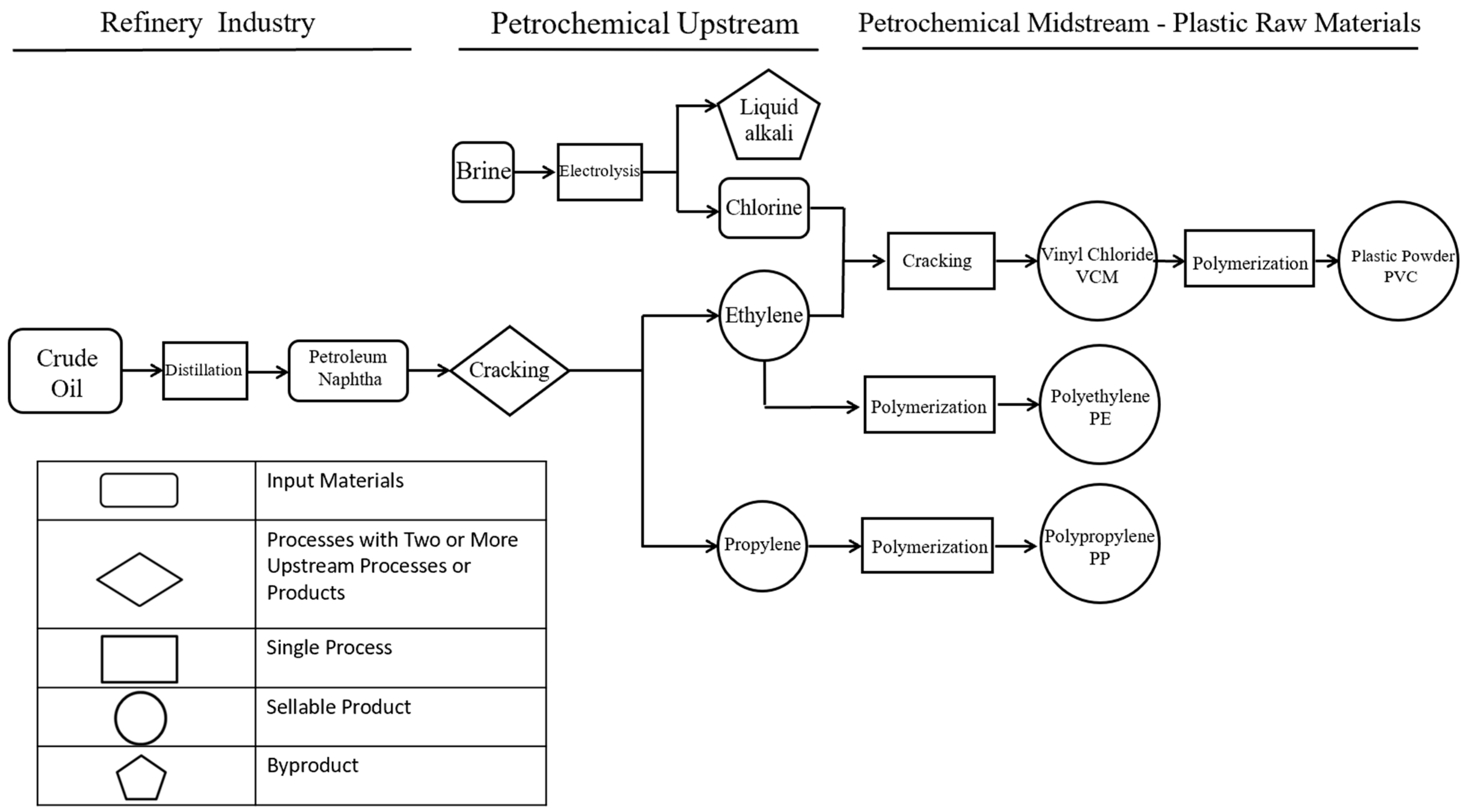
3.1. Production Process

The petrochemical industry refers to industries that use petroleum or natural gas as raw materials to produce chemical products, and the final products are called petrochemical products. The scope of the petrochemical industry includes upstream industries such as the production of basic raw materials such as ethylene, propylene, and butadiene, but does not include raw materials such as petroleum, natural gas, gasoline, and light oil; the petrochemical industry production process is based on refining crude oil, and by pressure distillation, petroleum naphtha is obtained, which is then cracked to produce basic petrochemical materials such as ethylene and propylene. After the above-mentioned raw materials are put in and go through steps such as polymerization, oxidation, and synthesis, the chemical raw materials of the midstream petrochemical industry can be produced, such as polyethylene (PE), polypropylene (PP), and polyvinyl chloride (PVC), which are the main materials used in plastics. These plastic raw materials can provide downstream manufacturers with various daily necessities, such as plastic products, rubber products, artificial fibers, cleaning products, and cosmetics, etc. Therefore, the midstream and upstream petrochemical manufacturing processes play an indispensable role in our lives. Figure 1 illustrates the transformation of crude oil into plastic raw materials through three stages: Refinery Industry, Petrochemical Upstream, and Petrochemical Midstream. Crude oil undergoes distillation to produce petroleum naphtha, which is then cracked into ethylene and propylene—key feedstocks for plastic production. The electrolysis of brine generates chlorine, which reacts with ethylene to form vinyl chloride monomer (VCM). These intermediates undergo polymerization to produce polyvinyl chloride (PVC), polyethylene (PE), and polypropylene (PP), essential plastic materials. The legend explains the symbols used to distinguish inputs, processes, products, and byproducts.

3.2. Research Assumptions

This research will take the upstream and midstream processes of the petrochemical industry as an example. Based on the capacity limits and demand forecasts of the process, this study will limit production at different parts of the process. The aim is to determine the target results of each model.

This research will exclude uncontrollable factors and maintain consistency, and will make the following research assumptions:

• There are six main products: ethylene (i = 1), propylene (i = 2), vinyl chloride (i = 3), plastic powder (i = 4), polyethylene (i = 5), and polypropylene (i = 6); there is one byproduct: liquid alkali. The unit prices of the above products are fixed during the production process.
• The costs of the main raw materials put into production remain unchanged during the production process.
• The quantity of products produced is equal to the quantity sold, and the model does not include any inventory.
• The products produced in the same production step will be produced at a certain production ratio.
• Labor costs will be paid in accordance with the first and second stage overtime rates as overtime hours increase, and in accordance with the government’s policies. Each stage rate will remain constant during the production process.
• In the carbon tax cost model, each unit of product produced is subject to a carbon tax, without setting an upper limit. That is, the amount of carbon tax depends on the quantity of products produced.

3.3. Objective Functions

This section introduces the primary objective functions of this study and the related constraints.

3.3.1. General Form of the Objective Functions

The primary objective functions of this study are outlined below. The first objective focuses on maximizing the profit, which is essential for business operations. The second objective addresses the current issue of carbon emissions, aiming to minimize emissions during the production process.

The profit function incorporates costs calculated using Activity-Based Costing (ABC), which enables more accurate cost tracing and allocation to determine more reasonable costs. Meanwhile, carbon emissions are measured based on the emissions generated per unit of production for each major product. As production volume increases, the total carbon emissions also rise proportionally.

The production volume of each product has opposing effects on the two objectives. Higher production volumes contribute to maximizing profits. Conversely, reduced production volumes align better with the second objective of minimizing carbon emissions.

Objective 1:

Profit Maximization

• Profit Maximization = Total Primary Product Revenue + Byproduct Revenue − Total Direct Material Cost − Total Direct Labor Cost − Total Output-Level Costs − Total Batch-Level Costs − Total Fixed Costs

$$\begin{gathered} Max Profit=\sum _{i=1}^6{P}_i{X}_i+QW-\sum _{i=1}^6\left(\sum _{m=1}^2{MC}_m{MU}_{im}\right)X_i-\left[{DL}_0+{\eta }_1\left({DL}_1-{DL}_0\right)+{\eta }_2\left({DL}_2-{DL}_0\right)\right] \\ -\sum _{i=1}^6\sum _{p=1}^6{EC}_p{MH}_{ip}{X}_i-\sum _{i=1}^6\sum _{b=1}^2{BC}_b{SH}_{ib}{N}_{ib}-F \end{gathered}$$

(1)

Symbol Descriptions:

$Max Profit$:	Maximizing Business Profit
$P_i$:	The unit selling price of product $i$ ($i=1~6$)
$X_i$:	The production quantity of product $i$ ($i=1~6$)
$i=1~6$:	The product categories include Ethylene (i = 1), Propylene (i = 2), Vinyl Chloride (i = 3), Plastic Powder (i = 4), Polyethylene (i =5), Polypropylene (i = 6)
$Q$:	The price of the byproduct (liquid alkali)
$W$:	The production quantity of the byproduct (liquid alkali)
$m=1~2$:	The raw materials include Petroleum ($m=1$), Salt ($m=2$)
${MC}_m$:	The cost per unit of raw material ($m=1~2$)
${MU}_{im}$:	The amount of raw material used to produce one unit of product i ($i=1~6$, $m=1~2$)
${DL}_0$:	The total direct labor cost at the point ${DLH}_0$ ${ DL}_0={WR}_0\times {DLH}_0$
${DL}_1$:	The total direct labor cost at the point ${DLH}_1$ ${DL}_1={DL}_0+{WR}_1\times ({DLH}_1-{DLH}_0)$
${DL}_2$:	The total direct labor cost at the point ${DLH}_2$ ${DL}_2={DL}_1+{WR}_2\times ({DLH}_2-{DLH}_1)$
${\eta }_1, {\eta }_2$:	This represents non-negative variables, with at most two adjacent variables being non-zero.
$p=1~6$:	The processes include Distillation and cracking ($p=1),$ Electrolysis ($p=2$), Cracking ($p=3$), Polymerization ($p=4$), Polymerization ($p=5$), Polymerization ($p=6$)
${EC}_p$:	The machine cost per hour in production process $p$
${MH}_{ip}$:	The number of machine hours required to produce product $i$ in process $p$ ($i=1~6$, $p=1~6$)
$b=1~2$:	The batch activities include Material delivery ($b=1$), Machine setup ($b=2$)
${BC}_b$:	The setup cost per hour in batch activity $b$ ($b=1~2$)
${SH}_{ib}$:	The number of setup hours required for each batch activity $b$ ($i=1~6$, $b=1~2$)
$N_{ib}$:	The batch number of product i produced in batch activity $b$ ($i=1~6$, $b=1~2$)
$F$:	Total fixed costs

Objective 2:

Carbon Emissions Minimization

Carbon Dioxide Emissions = Carbon emissions generated from the production of ethylene/propylene and their processed products + Carbon emissions generated from the production of vinyl chloride and its processed products.

$$Min {CO}_2=\sum _{i=1}^6{X}_i{\alpha }_i+(X_3+X_4){\beta }_i\gamma$$

(2)

Symbol Definition:

$Min {CO}_2$:	Minimizing carbon dioxide emissions.
${\alpha }_i, {\beta }_i$:	The carbon dioxide emission coefficient of the product (tons of CO2 per ton of production).
$\gamma$:	The geographical adjustment factor coefficient for vinyl chloride ($X_3$) and its processed products.

3.3.2. Constraints Related to Objective Functions

(1)

Direct Materials

This study assumes that the raw materials used in the petrochemical industry’s plastic production processes include petroleum (m = 1 m = 1 m = 1) and salt (m = 2 m = 2 m = 2). These costs are part of the overall profit and should be subtracted from the profit function. The following are the related cost functions and constraints. The maximum allowable raw material usage is the maximum value of this constraint.

Direct Material Cost Function:

$$\sum _{i=1}^6\left(\sum _{m=1}^2{MC}_m{MU}_{im}\right)X_i$$

The related constraints are as follows:

$$\sum _{i=1}^6\left({MU}_{im}{X}_i\right)\le {LMQ}_m$$

(3)

Symbol Descriptions:

${LMQ}_m$:

The upper limit of the m-th type of usable raw materials quantity.

(2)

Direct Labor

The labor hours used in this process include regular working hours as well as overtime hours. In this study, it is assumed that in the manufacturing process, the first three steps of the process—distillation and cracking ($p=1$), electrolysis ($p=2$), and cracking ($p=3$)—require manual supervision and other tasks. In cases where urgent orders arise or orders cannot be completed on time, overtime will occur, increasing the direct labor costs. As shown in Figure 2, it is assumed that the cost of direct labor varies as follows: The first stage reflects the payment during regular working hours, while the second and third stages represent overtime situations. If overtime extends beyond a certain number of hours, the payment per unit increases significantly. The amount of labor input and the production volume of products will determine the direct labor costs.

Direct labor cost function:

$$\left[{DL}_0+{\eta }_1\left({DL}_1-{DL}_0\right)+{\eta }_2\left({DL}_2-{DL}_0\right)\right]$$

The related constraints are as follows:

$$\sum _{i=1}^6\sum _{p=1}^3{SLH}_{ip}{X}_i\le \left[{DLH}_0+{\eta }_1\left({DLH}_1-{DLH}_0\right)+{\eta }_2\left({DLH}_2-{DLH}_0\right)\right]$$

(4)

$${\eta }_0-{\Omega }_1\le 0$$

(5)

$${\eta }_1-{\Omega }_1-{\Omega }_2\le 0$$

(6)

$${\eta }_2-{\Omega }_2\le 0$$

(7)

$${\eta }_0+{\eta }_1+{\eta }_2=1$$

(8)

$${\Omega }_1+{\Omega }_2=1$$

(9)

$${\Omega }_1, {\Omega }_2=0, 1$$

(10)

$$0\le {\eta }_0, {\eta }_1, {\eta }_2\le 1$$

(11)

Symbol Descriptions:

${SLH}_{ip}$:	The number of labor hours required to produce product $i$ in each process $p$. ($i=1~6$, $p=1~6$)
${\eta }_0, {\eta }_1, {\eta }_2$:	This represents non-negative variables, with at most two adjacent variables being non-zero.
${\Omega }_1, {\Omega }_2$:	This refers to binary variables (0 or 1), where only one of the two variables can be 1 at any given time.

(3)

Output Unit Level

The cost of manufacturing each unit of product in the process is traced back to the machine hours used in the production, which are allocated to this cost. In this study, it is assumed that all production processes require the use of machines for manufacturing. This process includes six steps: Distillation and cracking ($p=1$), Electrolysis ($p=2$), Cracking ($p=3$), Polymerization $(p=4$), Polymerization ($p=5$), Polymerization ($p=6$) The consumption of machine hours in each process is considered, and the production quantity affects the cost of this part of the process.

Output Unit Level Cost Function:

$$\sum _{i=1}^6\sum _{p=1}^6{EC}_p{MH}_{ip}{X}_i$$

The related constraints are as follows:

$$\sum _{i=1}^6\sum _{p=1}^6{MH}_{ip}{X}_i\le {MT}_p$$

(12)

Symbol Descriptions:

${MT}_p$:

The maximum available machine hours.

(4)

Batch Level

The costs generated by the production process due to batch activities are accounted for at this level. These costs include activities such as material handling, machine setup, quality inspections, packaging, and transportation. In this study, indirect costs are allocated not only based on machine hours but also considering the cost drivers related to batch activities. The cost for each product batch is calculated accordingly.

These batch-related costs may include the time required to adjust equipment when switching between batches, additional testing or inspection processes for specific batches, and inventory management costs between different batches. By breaking down these batch-related costs and allocating them accurately to each product batch, the total cost for each batch of products can be more precisely evaluated, thereby improving cost management accuracy and facilitating the establishment of more reasonable product pricing.

Batch Level Cost Function:

$$\sum _{i=1}^6\sum _{b=1}^2{BC}_b{SH}_{ib}{N}_{ib}$$

The related constraints are as follows:

$$X_i\le {QB}_{ib}{N}_{ib}$$

(13)

$$\sum _{i=1}^6{SH}_{ib}{N}_{ib}\le {TB}_b$$

(14)

Symbol Descriptions:

${QB}_{ib}$:	The quantity of product $i$ in each batch activity $b$.
${TB}_b$:	The available time (in hours) for handling batch activity $b$.

3.4. Model Assumptions

The following assumptions will be made for the different scenarios, including the basic model, the model with renewable energy use, the model with a continuous progressive carbon tax rate, and the model with a discontinuous progressive carbon tax rate. Each model is an extension of the basic model, with additional functions related to the specific scenario. The aim is to observe the results in terms of profit and carbon emissions under each scenario, as well as the differences between the four scenarios.

3.4.1. Basic Function

$$\begin{gathered} Max Profit=\sum _{i=1}^6{P}_i{X}_i+QW-\sum _{i=1}^6\left(\sum _{m=1}^2{MC}_m{MU}_{im}\right)X_i-\left[{DL}_0+{\eta }_1\left({DL}_1-{DL}_0\right)+{\eta }_2\left({DL}_2-{DL}_0\right)\right] \\ -\sum _{i=1}^6\sum _{p=1}^6{EC}_p{MH}_{ip}{X}_i-\sum _{i=1}^6\sum _{b=1}^2{BC}_b{SH}_{ib}{N}_{ib}-F \end{gathered}$$

(1)

$$Min {CO}_2=\sum _{i=1}^6{X}_i{\alpha }_i+(X_3+X_4){\beta }_i\gamma$$

(2)

This model serves as the comparison basis for other functional models and is also the functional model listed in Section 3.3.1 above.

3.4.2. Function with Renewable Energy Usage

$$\begin{gathered} Max Profit=\sum _{i=1}^6{P}_i{X}_i+QW-\sum _{i=1}^6\left(\sum _{m=1}^2{MC}_m{MU}_{im}\right)X_i-\left[{DL}_0+{\eta }_1\left({DL}_1-{DL}_0\right)+{\eta }_2\left({DL}_2-{DL}_0\right)\right] \\ -\sum _{i=1}^6\sum _{p=1}^6{EC}_p{MH}_{ip}{X}_i-\sum _{i=1}^6\sum _{b=1}^2{BC}_b{SH}_{ib}{N}_{ib}+C_S{RE}_s-F \end{gathered}$$

(15)

$$Min {CO}_2=\sum _{i=1}^6{X}_i{\alpha }_i+{(X}_3+X_4){\beta }_i\gamma -{RE}_S\phi$$

(16)

This section, in addition to the basic formula, explores the situation where circular economy practices are incorporated. As shown in Equations (15) and (16), the profit maximization objective includes the reduction in variable costs and the increase in fixed costs due to the use of renewable energy (SRF), while the carbon emissions minimization objective includes the reduction in carbon emissions from replacing coal-fired power generation with SRF. This model assumes that measures to reduce carbon emissions are implemented in the production process by substituting high-carbon coal with renewable energy for power generation. Since the use of renewable energy is still under development, the model assumes that SRF usage will only account for a portion of the production process. It also assumes that additional equipment will be required, thus increasing fixed costs. The reduction in carbon emissions due to the use of renewable energy to replace high-carbon coal is dependent on the production quantity. The following are the related constraints for using SRF:

$${RE}_S=(\sum _{i=1}^6{P}_i+Q)\sigma$$

(17)

Symbol Explanation:

$C_S$:	The cost savings per unit of using SRF to replace coal.
${RE}_s$:	The amount of SRF used in the production process.
$\phi$:	The amount of carbon emissions reduced per unit by replacing coal with SRF (tons of CO2 per ton of usage).
$\sigma$:	The correlation coefficient between the use of SRF and each product ($P_i$, $Q$).

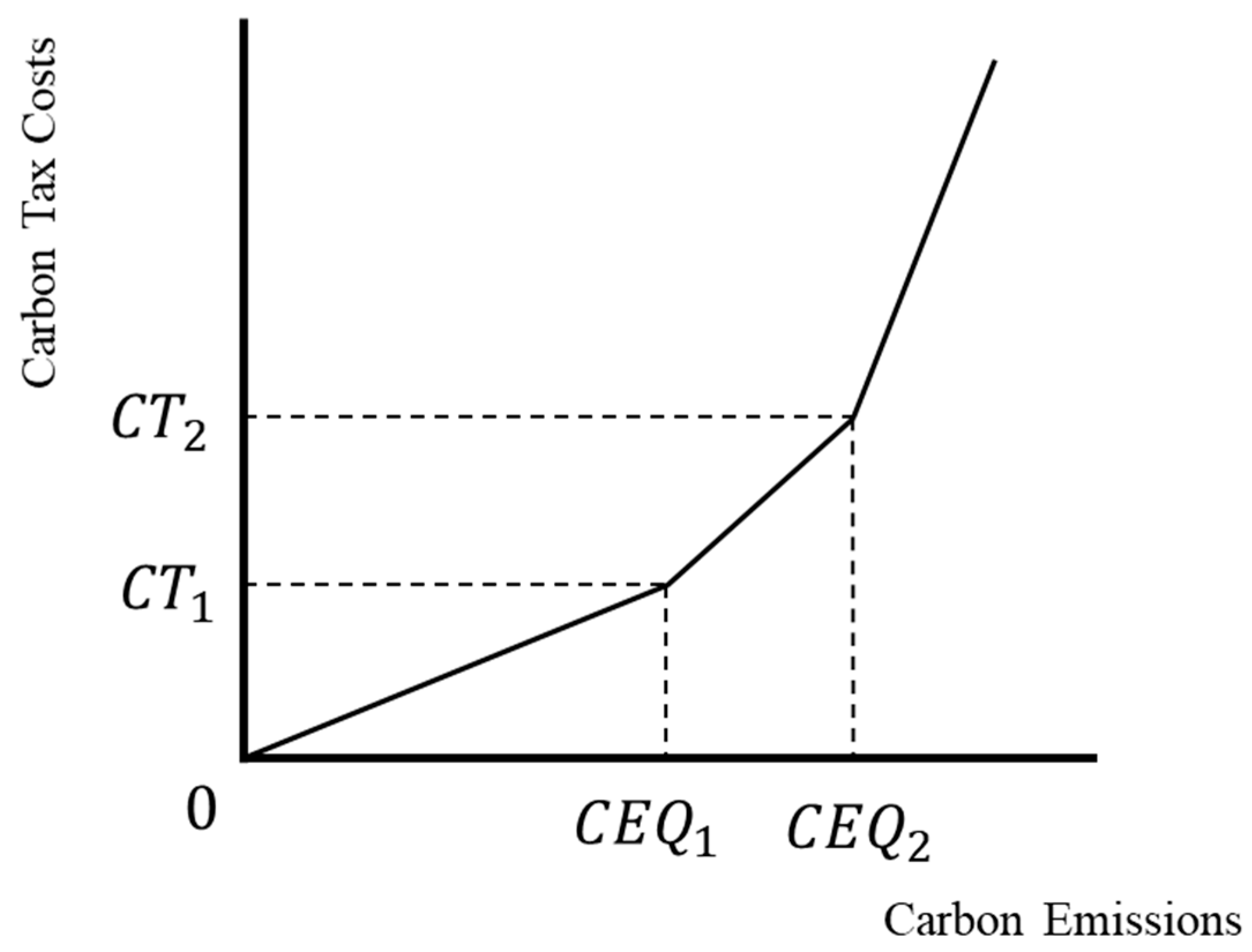
3.4.3. Carbon Tax Cost Function with Continuous Incremental Progressive Tax Rates

$$\begin{gathered} Max Profit=\sum _{i=1}^6{P}_i{X}_i+QW-\sum _{i=1}^6\left(\sum _{m=1}^2{MC}_m{MU}_{im}\right)X_i-\left[{DL}_0+{\eta }_1\left({DL}_1-{DL}_0\right)+{\eta }_2\left({DL}_2-{DL}_0\right)\right] \\ -\sum _{i=1}^6\sum _{p=1}^6{EC}_p{MH}_{ip}{X}_i-\sum _{i=1}^6\sum _{b=1}^2{BC}_b{SH}_{ib}{N}_{ib}-({\omega }_1{CT}_1+{\omega }_2{CT}_2+{\omega }_3{CT}_3)-F \end{gathered}$$

(18)

$$Min {CO}_2=\sum _{i=1}^6{X}_i{\alpha }_i+(X_3+X_4){\beta }_i$$

(2)

This section includes the cost of carbon tax, with a continuous incremental progressive tax rate. The carbon emissions generated by production will correspond to different carbon tax rates. As shown in Figure 3 and function (19), the carbon emission limits for the first and second stages are represented by ${CEQ}_1$ and ${CEQ}_2$, respectively. The corresponding carbon tax costs are ${CT}_1$ and ${CT}_2$. ${TR}_1$, ${TR}_2$, and ${TR}_3$ represent the carbon tax rates for the three stages, respectively.

$$f\left(q\right)=\left\{\begin{array}{cc}\hfill q\ast {TR}_1,& if 0 \le q\le {CEQ}_1\hfill \\ \hfill {CT}_1+\left(q-{CEQ}_1\right){TR}_2,& if {CEQ}_1<q\le {CEQ}_2\hfill \\ \hfill {CT}_2+\left(q-{CEQ}_2\right){TR}_3,& if {CEQ}_2<q\hfill \end{array}\right.$$

(19)

The related constraints are as follows:

$$TCT={\omega }_1{CT}_1+{\omega }_2{CT}_2+{\omega }_3{CT}_3$$

$$\sum _{i=1}^6\sum _{p=1}^6{CE}_{ip}{X}_i={\omega }_1{CEQ}_1+{\omega }_2{CEQ}_2+{\omega }_3{CEQ}_3$$

(20)

$${\omega }_0-{\epsilon }_1\le 0$$

(21)

$${\omega }_1-{\epsilon }_1-{\epsilon }_2\le 0$$

(22)

$${\omega }_2-{\epsilon }_2-{\epsilon }_3\le 0$$

(23)

$${\omega }_3-{\epsilon }_3\le 0$$

(24)

$${\omega }_0+{\omega }_1+{\omega }_2+{\omega }_3=1$$

(25)

$${\epsilon }_1+{\epsilon }_2+{\epsilon }_3=1$$

(26)

$$0\le {\omega }_0, {\omega }_1, {\omega }_2, {\omega }_3\le 1$$

(27)

$${\epsilon }_1, {\epsilon }_2, {\epsilon }_3=0, 1$$

(28)

Symbol Explanation:

$TCT$:	The total carbon tax cost of the company
${\omega }_0, {\omega }_1, {\omega }_2, {\omega }_3$:	Represents a binary variable (0, 1), where at most two adjacent variables are non-zero.
${CT}_1$:	The carbon tax cost at the carbon emission level of ${CEQ}_1$
${CT}_2$:	The carbon tax cost at the carbon emission level of ${CEQ}_2$
${CT}_3$:	The carbon tax cost at the carbon emission level of ${CEQ}_3$
${CE}_{ip}$:	The carbon emission per unit of product $i$ in process $p$. ($i=1~6$, $p=1~6$)
${CEQ}_1$:	The carbon emission in the first stage.
${CEQ}_2$:	The carbon emission in the second stage.
${CEQ}_3$:	The carbon emissions exceeding the second stage ${CEQ}_2$, with no upper limit for this stage.
${\epsilon }_1, {\epsilon }_2, {\epsilon }_3$:	It is a binary variable (0, 1), with only one of the three items being 1.

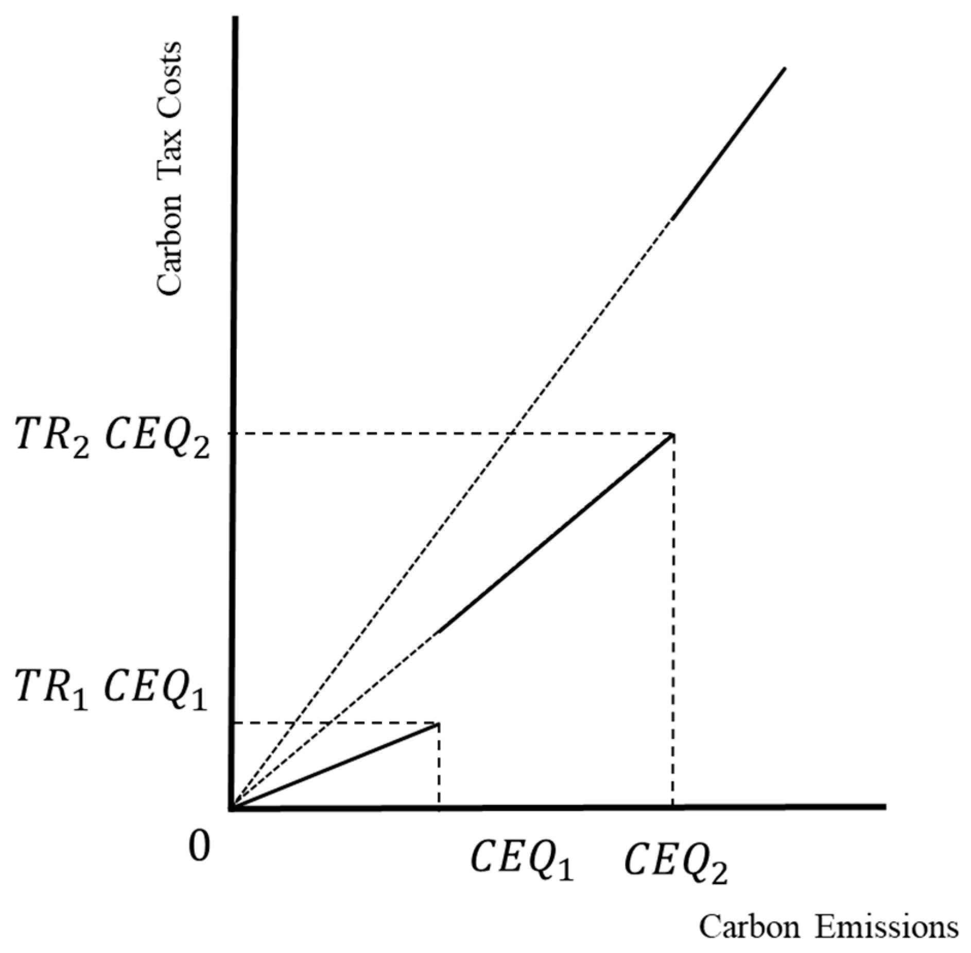
3.4.4. Carbon Tax Cost Function with Discontinuous Incremental Progressive Tax Rate

$$\begin{gathered} Max Profit=\sum _{i=1}^6{P}_i{X}_i+QW-\sum _{i=1}^6\left(\sum _{m=1}^2{MC}_m{MU}_{im}\right)X_i-\left[{DL}_0+{\eta }_1\left({DL}_1-{DL}_0\right)+{\eta }_2\left({DL}_2-{DL}_0\right)\right] \\ -\sum _{i=1}^6\sum _{p=1}^6{EC}_p{MH}_{ip}{X}_i-\sum _{i=1}^6\sum _{b=1}^2{BC}_b{SH}_{ib}{N}_{ib}-({{\lambda }_{1}DCT}_1+{\lambda }_2{DCT}_2+{\lambda }_3{DCT}_3)-F \end{gathered}$$

(29)

$$Min {CO}_2=\sum _{i=1}^6{X}_i{\alpha }_i+(X_3+X_4){\beta }_i$$

(2)

Figure 4 illustrates the discontinuous carbon tax imposition method, where different tax rates are applied based on the amount of carbon emissions. The emissions are divided into three stages, with upper limits for the first two stages being ${CEQ}_1$ and ${CEQ}_2$, respectively. Once the carbon emissions exceed a stage, a higher tax rate is applied. The tax rates are ${TR}_1$, ${TR}_2$, and ${TR}_3$, and the costs are calculated by multiplying the carbon emissions by the corresponding tax rate for each stage, such as $q\ast {TR}_1$. The related graph and equations are shown as follows:

$$f\left(q\right)=\left\{\begin{array}{cc}\hfill q\ast {TR}_1,& if 0 \le q\le {CEQ}_1\hfill \\ \hfill q\ast {TR}_2,& if {CEQ}_1<q\le {CEQ}_2\hfill \\ \hfill q\ast {TR}_3,& if {CEQ}_2<q\hfill \end{array}\right.$$

(30)

The related constraints are as follows:

$$TDCT={\lambda }_1{DCT}_1+{\lambda }_2{DCT}_2+{\lambda }_3{DCT}_3$$

$$\sum _{i=1}^6\sum _{p=1}^6{CE}_{ip}{X}_i={\lambda }_1+{\lambda }_2+{\lambda }_3$$

(31)

$$0\le {\lambda }_1\le {\mu }_1{CEQ}_1$$

(32)

$$0<{\lambda }_2\le {\mu }_2{CEQ}_2$$

(33)

$${\lambda }_3>{\mu }_3{CEQ}_2$$

(34)

$${\mu }_1+{\mu }_2+{\mu }_3=1$$

(35)

$${\mu }_1, {\mu }_2, {\mu }_3=0, 1$$

(36)

Symbol Explanation:

${\lambda }_1, {\lambda }_2, {\lambda }_3$:	The total carbon emissions falling within the first, second, or third phase.
${DCT}_1$, ${DCT}_2$, ${DCT}_3$:	The tax rate for the discontinuous carbon tax.
${\mu }_1, {\mu }_2, {\mu }_3$:	Represents a binary variable (0, 1), where only one of the three can be 1.

4. Analysis of Research Results

4.1. ε-Constraint Method

This study will use the ε-constraint method from unbiased multi-objective programming. The $\epsilon$–Constraint Method involves restricting other objectives to a fixed value while optimizing a single objective. In other words, by limiting other objectives to different target values, a series of optimal solutions for a single objective can be obtained, forming an approximate set of non-dominated solutions.

Based on the multi-objective programming approach outlined above, the first objective function, profit, is set as the single objective, while the second objective, carbon emissions, is constrained to different target values to obtain the optimal solution. Regarding the upper and lower limits, the core of multi-objective programming is to simultaneously consider multiple objectives, which are often in conflict with each other. By setting upper and lower limits, it ensures that while optimizing the primary objective, the other objectives remain within acceptable ranges, thus achieving a balance between the objectives. Furthermore, setting the upper and lower limits effectively controls the degree of deviation in the objectives. Therefore, for the carbon emission minimization, the upper and lower limits for the respective functions in each model are as follows:

(1)

Basic model: 5497.604~62,308.96 ton.

(2)

Renewable energy model: 4006.878~61,911.93 tons.

(3)

Carbon tax cost model with continuous incremental progressive tax rate: 5754.006~62,432.71 tons.

(4)

Carbon tax cost model with discontinuous incremental progressive tax rate: 4675.262~56,600.00 tons.

Each model will select the value of ${\epsilon }_t$ within the above limits, applying this value to the second objective, carbon emissions, making it one of the constraints in order to obtain the optimal profit solution for that ${\epsilon }_t$ value. The relevant function, using the basic model as an example, is shown as follows:

Objective Function:

$$\begin{gathered} Max Profit=\sum _{i=1}^6{P}_i{X}_i+QW-\sum _{i=1}^6\left(\sum _{m=1}^2{MC}_m{MU}_{im}\right)X_i+\left[{DL}_0+{\eta }_1\left({DL}_1-{DL}_0\right)+{\eta }_2\left({DL}_2-{DL}_0\right)\right] \\ -\sum _{i=1}^6\sum _{p=1}^6{EC}_p{MH}_{ip}{X}_i+\sum _{i=1}^6\sum _{b=1}^2{BC}_b{SH}_{ib}{N}_{ib}-F \end{gathered}$$

(1)

Constraints:

$$\sum _{i=1}^6{X}_i{\alpha }_i+(X_3+X_4){\beta }_i\gamma \le {\epsilon }_t$$

(37)

4.2. Illustrative Model Data

The products are as follows: Product 1: ethylene, Product 2: propylene, Product 3: vinyl chloride, Product 4: plastic powder, Product 5: polyethylene, Product 6: polypropylene, and byproduct: liquid alkali. The related illustrative data used in this paper are shown in

Table 3. Parameters of the Illustration.

Symbols

Products

Byproducts

Available Resources Limit

Ethylene (i = 1)

Propylene (i = 2)

Vinyl Chloride (i = 3)

Plastic Powder (i = 4)

Polyethylene (i = 5)

Polypropylene (i = 6)

Liquid Alkali

Sales Price per Metric Ton

$P_i, Q$

TWD 30,000

TWD 32,000

TWD 41,500

TWD 45,300

TWD 37,000

TWD 38,400

TWD 4700

Main Costs

Direct Material Input

Naphtha

m = 1

${MC}_1$ = 19,500 TWD/ton

${MU}_{i1}$

1.47

1.5

1.764

1.911

1.746

1.8

0

2,601,411

Salt

m = 2

${MC}_2$ = 4600 TWD/ton

${MU}_{i2}$

0

0

1

1

0

0

0.5

457,450

Direct labor hours

Distillation Cracking

p = 1

1.5

1.5

1.5

1.5

1.5

1.5

Electrolysis

p = 2

1

Cracking

p = 3

0.5

0.5

Output per unit operation

Machine hours

Distillation Cracking

p = 1

${MC}_P$ = 150 TWD/Machine hours

${MH}_{i1}$

5

10

5

5

5

10

3,325,500

Electrolysis

p = 2

${MH}_{i2}$

2

340,000

Cracking

p = 3

${MH}_{i3}$

2.27

2.27

485,800

Polymerization

p = 4

${MH}_{i4}$

3.03

535,500

Polymerization

p = 5

${MH}_{i5}$

1.01

123,000

Polymerization

p = 6

${MH}_{i6}$

1.01

99,600

Symbols

Products

Byproducts

Available Resources Limit

Ethylene (i = 1)

Liquid Alkali (i = 2)

Vinyl Chloride (i = 3)

Plastic Powder (i = 4)

Polyethylene (i = 5)

Polypropylene (i = 6)

Liquid Alkali

Batch Level Operations

Material Distribution

b = 1

${BC}_1$ = 15,000 TWD/Number of Deliveries

${SH}_{i1}$

1

2000

${MU}_{i2}$

10,000

Machine Maintenance

b = 2

${BC}_2$ = 3400 TWD/Maintenance Hours

${SH}_{i2}$

2

2

10

12

5

5

10

50,000

$n_{i2}$

600

600

400

800

300

300

500

Direct Labor Cost

Cost

${DL}_0$ = TWD 78,031,200

${DL}_1$ = TWD 130,585,000

${DL}_2$ = TWD 165,105,360

Labor Hours

${DLH}_0$ = 426,400

${DLH}_1$ = 533,000

${DLH}_2$ = 539,560

Wage Rate

183 TWD/hr

245 TWD/h

306 TWD/h

Renewable Energy Use

SRF Usage Reduces Carbon Emissions

0.000788 tons per production unit

Reduce variable cost ratio

15% per machine hour cost

Increase fixed cost ratio

55%

Carbon tax

Unit carbon emissions

${\alpha }_i$

0.04

0.04

0.1764

0.2164

0.0751

0.0751

0

Segment costs

${CT}_1$ = TWD 10,500,000

${CT}_2$ = TWD 28,300,000

${CT}_3$ = TWD 560,000,000

Segment carbon emission limits

${CEQ}_1$ = 35,000

${CEQ}_2$ = 56,600

${CEQ}_3$ = 70,000

Segment tax rates

${TR}_1$ = 300 TWD/ton

${TR}_2$ = 500 TWD/ton

${TR}_3$ = 800 TWD/ton

. The respective prices are TWD 30,000, TWD 32,000, TWD 41,500, TWD 45,300, TWD 37,000, TWD 38,400, and TWD 4700. The unit costs of raw materials are naphtha 19,500 TWD/ton, salt 4600 TWD/ton. The labor cost wage rates are 183 TWD/hr for normal working hours, 245 TWD/h for overtime in the first stage, and 306 TWD/hr for overtime in the second stage. The machine operation hour limits for each process are as follows: Distillation and Cracking (p = 1) 3,325,500 h, Electrolysis (p = 2) 340,000 h, Cracking (p = 3) 485,800 h, Polymerization (p = 4) 535,500 h, Polymerization (p = 5) 123,000 h, and Polymerization (p = 6) 99,600 h. The carbon emission reduction per unit of renewable energy used is 0.000788 tons/unit of production. The carbon tax rates for the first, second, and third stages are 300 TWD/ton, 500 TWD/ton, and 800 TWD/ton, respectively. Each model will be calculated using the above data.

4.3. Results Comparison and Analysis

This section explains the profit trends under four models when minimizing carbon emissions as the second objective function. It also analyzes the results. Furthermore, it compares the differences in profits and product output across the models under three hypothetical carbon tax levels by restricting carbon emissions to specific values.

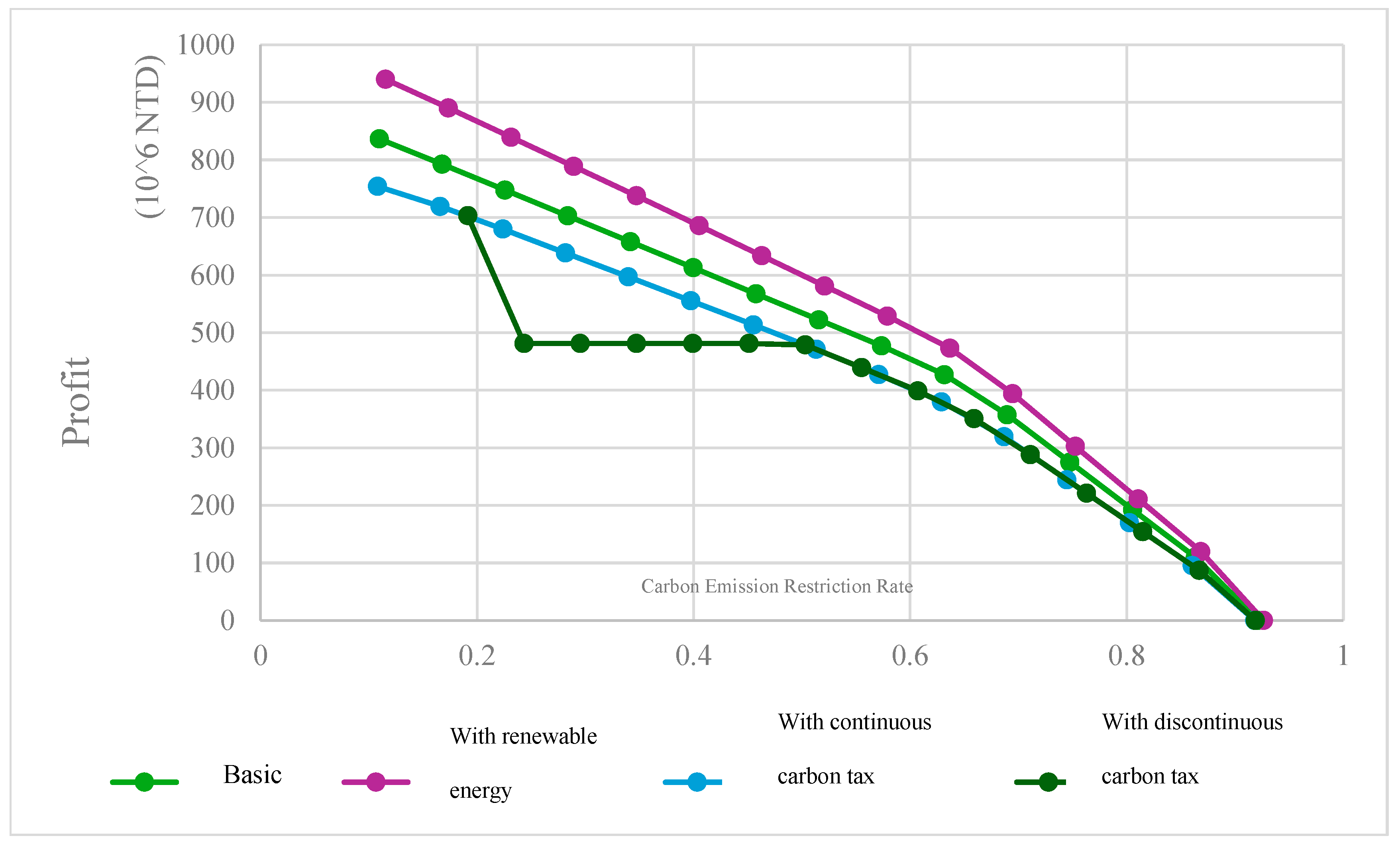
4.3.1. Model Profit Analysis

This part uses LINGO 20.0 to calculate the maximum and minimum carbon emissions for each model, determining the upper and lower bounds of this objective function.

Table 4. Maximum and minimum values of each model.

	Basic Model		Model with Renewable Energy
	Max Profit	Min Carbon Emissions	Max Profit	Min Carbon Emissions
Profit	TWD 836,612,800	62,308.96 (tons)	TWD 940,166,300	61,911.93 (tons)
Carbon Emissions	TWD 13,649.5	5497.604 (tons)	TWD 620.25	5149.618 (tons)
	Model with Continuous Incremental Progressive Tax Rates		Model with Discontinuous Incremental Progressive Tax Rates
	Max Profit	Min Carbon Emissions	Max Profit	Min Carbon Emissions
Profit	TWD 754,106,000	62,432.71 (tons)	TWD 703,262,000	56,600 (tons)
Carbon Emissions	TWD 521.67	5714.981 (tons)	TWD 197,627.3	5677.096 (tons)

provides the numerical upper and lower limits for each model.

Taking the basic model as an example, the value at the position of profit and Max profit represents the optimal solution of TWD 836,612,800, achieved when only profit is considered as the objective. On the other hand, the value at the position of carbon emissions and Min carbon emissions is the solution of 5497.604 tons, obtained when minimizing carbon emissions is the sole objective.

The carbon emissions value of 62,308.96 tons is calculated based on the production output that achieves the maximum profit of TWD 836,612,800. The maximum profit value of TWD 13,649.5 corresponds to the condition where the minimum carbon emissions of 5497.604 tons are applied.

Based on the above data, using the ε-constraint method, the profit variations in each model under the condition of minimizing carbon emissions are analyzed. Figure 5 shows the profit variation under the constraint of the second objective, carbon emissions. The horizontal axis represents the carbon emission restriction rate (%), where the emission limits are converted to restriction rates, ranging from 0 to 70,000 tons. Notably, 70,000 tons is the upper limit of carbon emissions set in this study’s carbon tax scenario. When the emission limit is set at 70,000 tons, the restriction rate is 0%; conversely, when the limit is 0 tons, the restriction rate is 100%. The vertical axis represents profit (TWD).

From the figure, the following observations can be made:

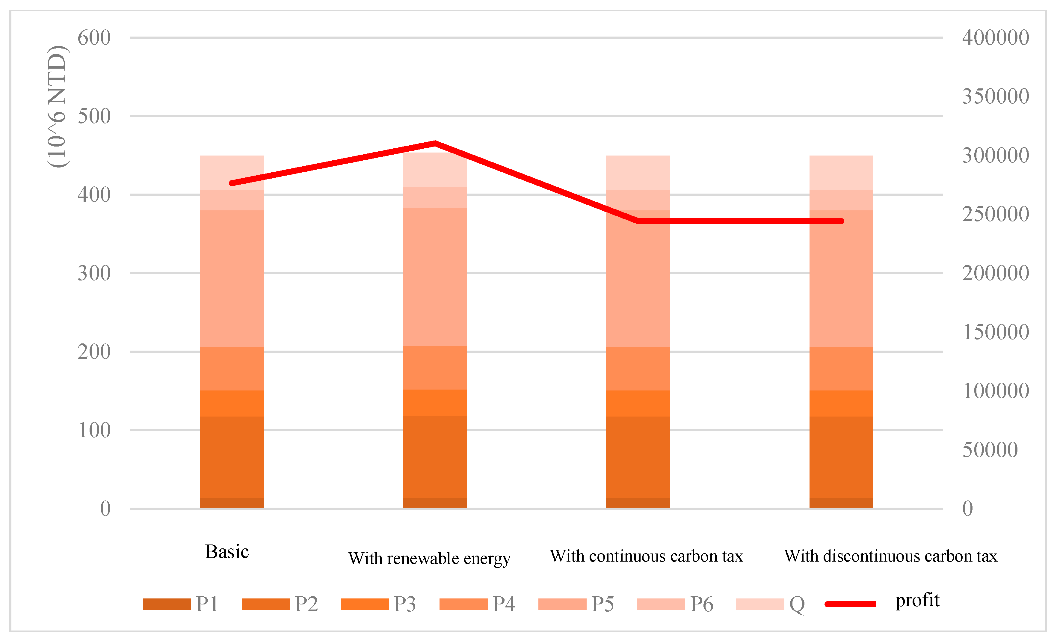
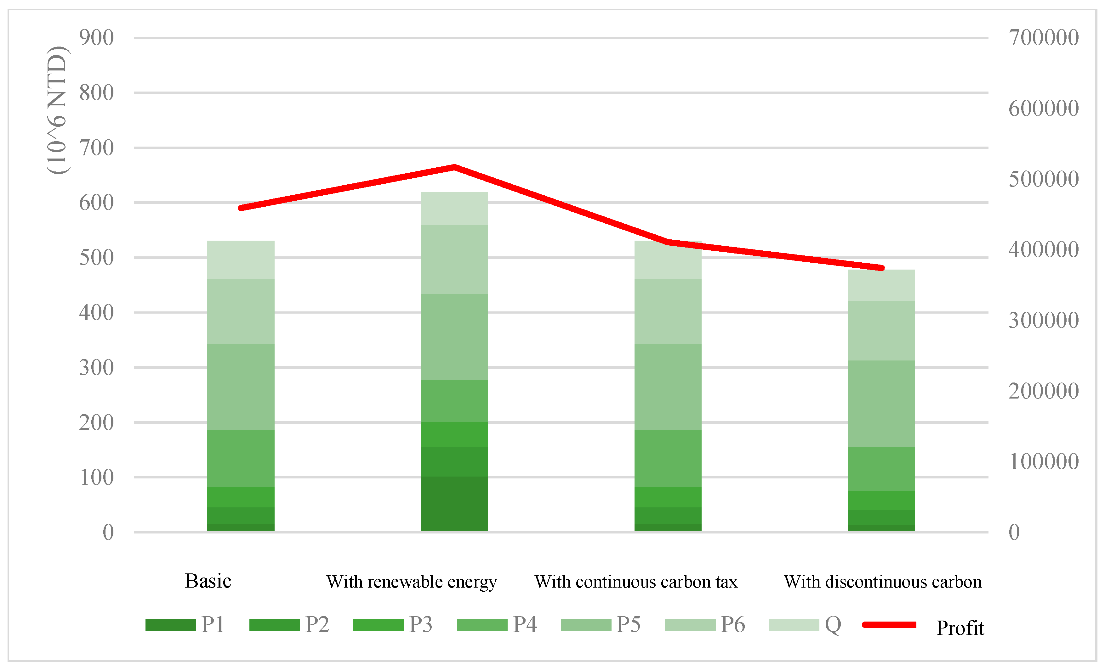
(1)

As the restriction rate on carbon emissions increases, the profit of all models shows a downward trend.

(2)

The model incorporating renewable energy consistently achieves the highest profit under any given carbon emission restriction. By utilizing renewable energy in production processes, companies can reduce some carbon emissions. Therefore, under the same carbon emission restrictions, this model can produce more products and achieve relatively higher profits compared to other models.

(3)

The basic model, as it does not involve carbon tax imposition, has higher profits than the two models with carbon tax. Moreover, as the carbon tax amount increases, the profit gap between the basic model and the continuous incremental progressive tax cost model widens under higher carbon emissions.

(4)

For the two models with carbon tax costs, both are subject to a tax rate of 300 TWD/ton during the first stage of carbon taxation. Thus, their profits remain identical when emissions are below 35,000 tons. However, in the second stage, the discontinuous incremental progressive tax cost model applies a higher tax rate of 500 TWD/ton to all emissions. Consequently, when the emission limits range between 35,001 and 56,599 tons, to maximize profits, the total product emissions remain at 35,000 tons, with profits maintained between TWD 481,157,800 and TWD 481,158,000. This strategy avoids the additional tax burden that would otherwise reduce profits.

Table 5. Profit of the discontinuous incremental progressive tax cost model under second-stage carbon taxation.

Carbon Emission Restriction Rate (%)	Carbon Emission Limit (tons)	Profit
24.3390718	≤52,962.64971	TWD 481,158,000
29.5352865	≤49,325.29943	TWD 481,157,900
34.7315012	≤45,687.94914	TWD 481,157,900
39.9277159	≤42,050.59886	TWD 481,158,000
45.1239306	≤38,413.24857	TWD 481,157,800

illustrates the emission limits and corresponding profits under the second-stage tax rate for the discontinuous incremental progressive tax cost model.

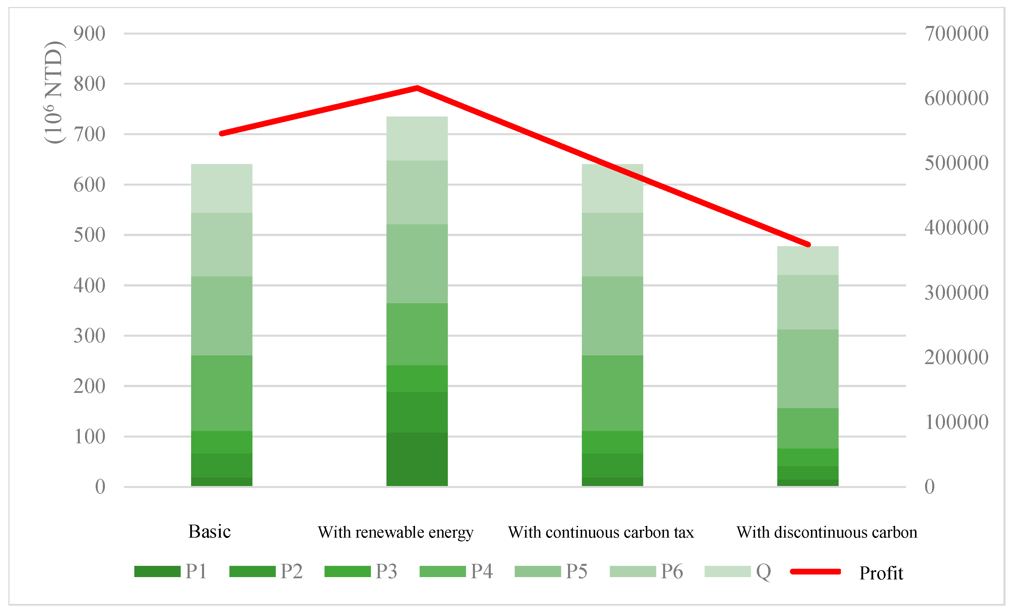
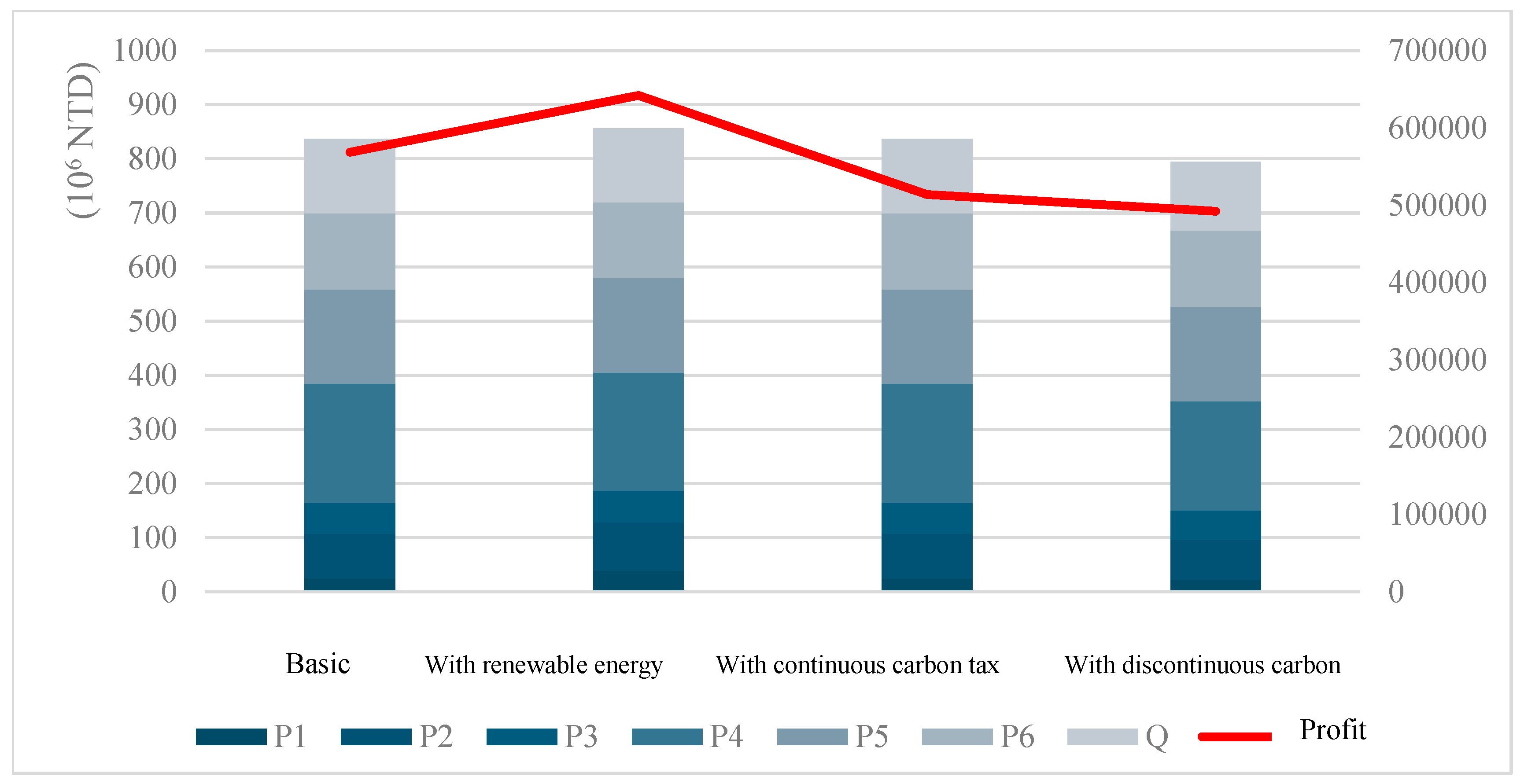
(5)

In the second stage of carbon taxation, the tax rate is already set at a high and stable level. Increased production leads to higher carbon tax costs, which offset the additional profits from increased production. Hence, under the trade-off between minimizing carbon emissions and maximizing profits, the emission limits in this stage keep profits stable. Similarly, when the emission limits exceed 56,600 tons up to 70,000 tons, corresponding to the third stage of taxation, the same pattern is observed. Examples of this situation will be discussed in Section 4.3.2.

4.3.2. Model Output Analysis

This section analyzes the results of minimizing carbon emissions under a fixed value for the second objective, examining profits and product output across four models. The values considered are drawn from three assumed carbon tax stages, with upper limits set as follows: first stage, 35,000 tons; second stage, 56,600 tons; and third stage, 70,000 tons. Two values are randomly selected from each stage for analysis to ensure comparative consistency. The models are represented numerically from Model 1 to Model 4, corresponding to the following names: basic model (Model 1), model with renewable energy (Model 2), continuous incremental tax rate model (Model 3), and discontinuous incremental tax rate model (Model 4). The primary axis (left) in the graph represents profit values, while the secondary axis (right) represents product production quantities.

A.

Values within Carbon Emission Quantity 25,000 and 30,000

In this stage, the fixed carbon emission limit is set between 0 and 35,000 tons. Here, two values—25,000 tons and 30,000 tons—are examined.

Table 6. Data for carbon emission limit ≤ 25,000 tons.

	Model 1	Model 2	Model 3	Model 4
Profit	TWD 414,482,500	TWD 465,254,700	TWD 366,310,000	TWD 366,310,000
Ethylene ($P_1$)	9198	9277	9198	9198
Propylene ($P_2$)	69,243	69,839	69,243	69,243
Chloroethane ($P_3$)	22,083	22,265	22,083	22,083
Plastic Powder ($P_4$)	36,800	37,123	36,800	36,800
Polyethylene ($P_5$)	11,5876	11,6873	11,5876	11,5876
Polypropylene ($P_6$)	17,325	17,473	17,325	17,325
Liquid Alkali ($Q$)	29,150	29,400	29,150	29,150
Total Product Output	29,9675	30,2250	29,9675	29,9675
Actual Carbon Emissions	25,000.00	24,999.98	25,000.00	25,000.00

and Figure 6 are the results for data carbon emission ≤ 25,000 tons;

Table 7. Data for carbon emission limit ≤ 30,000 tons.

	Model 1	Model 2	Model 3	Model 4
Profit	TWD 478,628,300	TWD 535,508,300	TWD 426,882,800	TWD 426,882,500
$\mathrm{Ethylene} (P_1$)	10,059	20,393	10,059	10,059
$\mathrm{Propylene} (P_2$)	19,097	19,800	19,097	19,094
$\mathrm{Chloroethane} (P_3$)	24,486	25,186	24,486	24,489
$\mathrm{Plastic} \mathrm{Powder} (P_4$)	44,800	42,181	44,800	44,797
$\mathrm{Polyethylene} (P_5$)	121,782	121,782	121,782	121,782
$\mathrm{Polypropylene} (P_6$)	75,551	78,808	75,551	75,554
$\mathrm{Liquid} \mathrm{Alkali} (Q$)	34,300	33,350	34,300	34,300
Total Product Output	33,0075	34,1500	33,0075	33,0075
Actual Carbon Emissions	30,000.00	29,999.99	30,000.00	29,999.98

and Figure 7 are the results for data carbon emission ≤ 30,000 tons. According to the data, production across all models is comparable. Even with a carbon emission limit of 25,000 tons, the continuous incremental tax rate model (Model 3) and the discontinuous incremental tax rate model (Model 4) show similar product outputs as the basic model (Model 1). This suggests that in this stage of carbon taxation, apart from the reduction in profits due to carbon tax impacts on Models 3 and 4, there is no significant effect on production. Specifically, since Models 3 and 4 operate within the first carbon tax stage without being influenced by continuous or discontinuous tax rates, the profit outcomes are nearly identical. For instance, with a carbon emission limit of 30,000 tons, profits for Models 3 and 4 are TWD 426,882,800 and TWD 426,882,500, respectively, while at a 25,000-ton limit, the profit value is TWD 366,310,000 for all three models.

B.

Values within Carbon Emission Quantity 40,000 and 50,000

When carbon emissions are restricted between 35,000 and 56,600 tons, Model 2 (which includes the use of renewable energy) exhibits the highest profit and production output. Model 1 (basic model) and Model 3 (continuous progressive carbon tax) show minimal differences in production quantities, even at carbon limits of 40,000 and 50,000 tons, where their product outputs are identical.

Table 8. Data for carbon emission limit ≤ 40,000 tons.

	Model 1	Model 2	Model 3	Model 4
Profit	TWD 590,125,200	TWD 664,616,200	TWD 527,879,800	TWD 481,157,800
$\mathrm{Ethylene} (P_1$)	12,227	79,143	12,227	11,194
$\mathrm{Propylene} (P_2$)	23,182	41,997	23,182	20,988
$\mathrm{Chloroethane} (P_3$)	29,244	35,498	29,244	27,094
$\mathrm{Plastic} \mathrm{Powder} (P_4$)	80,442	59,139	80,442	62,392
$\mathrm{Polyethylene} (P_5$)	121,782	121,782	121,782	121,782
$\mathrm{Polypropylene} (P_6$)	91,498	97,091	91,498	83,700
$\mathrm{Liquid} \mathrm{Alkali} (Q$)	54,300	46,850	54,300	44,300
Total Product Output	41,2675	481,500	412,675	371,450
Actual Carbon Emissions	39,999.98	39,999.98	39,999.98	34,999.99

and Figure 8 are the results for data carbon emission ≤40,000 tons;

Table 9. Data for carbon emission limit ≤ 50,000 tons.

	Model 1	Model 2	Model 3	Model 4
Profit	TWD 701,221,400	TWD 791,857,900	TWD 635,614,800	TWD 481,157,900
Ethylene ($P_1$)	14,393	83,880	14,393	11,194
Propylene ($P_2$)	37,200	62,832	37,200	20,989
Chloroethane ($P_3$)	34,816	41,115	34,816	27,093
Plastic Powder ($P_4$)	116,785	95,841	116,785	62,393
Polyethylene ($P_5$)	121,782	121,782	121,782	121,782
Polypropylene ($P_6$)	98,224	98,400	98,224	83,699
Liquid Alkali ($Q$)	75,050	67,800	75,050	44,300
Total Product Output	498,250	571,650	498,250	371,450
Actual Carbon Emissions	49,999.99	49,999.79	49,999.99	34,999.99

and Figure 9 are the results for data carbon emission ≤50,000 tons.

Model 4, which includes a non-continuous progressive carbon tax, demonstrates similar profit and production quantities at carbon limits differing by 10,000 tons. For instance, when the limit is 46,000 tons, the profit is TWD 481,157,800, and at 56,600 tons, the profit is TWD 481,157,900. This illustrates that Model 4 maintains consistent production and profits despite variations in carbon emission limits within the second tax stage.

C.

Values within Carbon Emission Quantity 60,000 and 65,000

The restrictions in this phase range from 56,600 tons to 70,000 tons, with specific values set at 60,000 tons and 65,000 tons. Under the carbon tax cost model with a discontinuous incremental progressive tax rate, when the carbon emission limit increases from 60,000 tons to 65,000 tons, the other three models continue to increase both profits and emissions, reaching their maximum production and profit levels.

Table 10. Data related to carbon emission limit ≤ 60,000 tons.

	Model 1	Model 2	Model 3	Model 4
Profit	TWD 811,996,300	TWD 917,234,200	TWD 733,925,100	TWD 703,290,700
Ethylene ($P_1$)	16,788	26,999	16,788	15,981
Propylene ($P_2$)	58,043	62,957	58,043	50,822
Chloroethane ($P_3$)	39,948	41,100	39,948	38,199
Plastic Powder ($P_4$)	154,376	152,618	154,376	141,581
Polyethylene ($P_5$)	121,782	121,782	121,782	121,782
Polypropylene ($P_6$)	98,613	98,219	98,613	98,610
Liquid Alkali ($Q$)	96,200	95,900	96,200	89,000
Total Product Output	585,750	599,575	585,750	555,975
Actual Carbon Emissions	59,998.70	59,999.99	59,998.70	56,599.99

and Figure 10 are the results for data carbon emission ≤60,000 tons;

Table 11. Data related to carbon emission limit ≤ 65,000 tons.

	Model 1	Model 2	Model 3	Model 4
Profit	TWD 836,612,800	TWD 940,166,300	TWD 754,106,000	TWD 703,290,700
Ethylene ($P_1$)	17,131	17,131	17,104	15,981
Propylene ($P_2$)	62,619	62,619	62,363	50,822
Chloroethane ($P_3$)	41,115	41,115	41,049	38,199
Plastic Powder ($P_4$)	163,511	163,511	164,789	141,581
Polyethylene ($P_5$)	120,861	120,861	119,132	121,782
Polypropylene ($P_6$)	98,613	98,613	98,613	98,610
Liquid Alkali ($Q$)	101,300	101,300	101,900	89,000
Total Product Output	605,150	605,150	604,950	555,975
Actual Carbon Emissions	62,308.96	61,911.93	62,432.71	56,599.99

and Figure 11 are the results for data carbon emission ≤65,000 tons.

Examining the performance of the models under the 65,000-ton emission limit reveals no significant restrictive effects on the basic model, the model incorporating renewable energy, or the carbon tax cost model with a continuous incremental progressive tax rate. These models have already achieved their optimal production and profit levels at this emission cap, indicating that the efficiency of current production processes has been maximized at this emission level. If further reduction in carbon emissions is desired through emission limits, lower emission caps should be considered, or alternative emission reduction measures should be introduced to promote higher efficiency in reductions.

For the discontinuous carbon tax model, the carbon emission limits in this phase lead to an increase in production and profit values compared to the second phase, reaching TWD 703,290,700. However, due to the carbon tax rate rising to 800 TWD per ton, the emission levels remain capped at 56,599.99 tons to avoid higher carbon tax charges, regardless of whether the emission limit is set at 60,000 or 65,000 tons.

The results indicate that profitability and carbon emissions are strongly influenced by the choice of carbon tax model. As shown in the tables and figures, the basic model achieves the highest profits but also generates the most carbon emissions since it does not include a carbon tax. Conversely, the model incorporating renewable energy consistently maintains higher profits compared to models with carbon tax costs, as the use of renewable energy helps reduce carbon emissions while allowing for more production under the same restrictions.

The continuous incremental progressive tax model and the discontinuous incremental progressive tax model exhibit different trends in profitability. When emissions remain under 35,000 tons, both models maintain identical profits since they are subject to the same carbon tax rate. However, as shown in Table 4, once emissions exceed this threshold, the discontinuous tax model applies a significantly higher rate of 500 TWD per ton, forcing firms to limit emissions at 35,000 tons to avoid excessive taxation. This results in a stable profit level of TWD 481,157,800 to TWD 481,158,000, demonstrating that firms strategically adjust production to optimize profits while complying with tax regulations.

At higher carbon emission levels (above 56,600 tons), models reach their maximum profit and production limits, as seen in Table 9 and Table 10. The discontinuous incremental tax model effectively limits emissions by maintaining a cap of 56,599.99 tons, even when emission limits increase, showing its strong emission control effect. Meanwhile, the basic model, renewable energy model, and continuous tax model all maximize production, indicating that their respective carbon tax structures do not sufficiently incentivize further emissions reduction at this stage. These trends emphasize that carbon tax structures significantly impact both production decisions and emission levels, with discontinuous tax policies proving to be the most effective in controlling emissions while maintaining profitability at a stable level.

In this section analyzing the situation with a specific carbon emission limit, this study finds that models incorporating renewable energy consistently achieve the highest profits, as the use of renewable energy reduces carbon emissions, allowing for greater production under the same restrictions. Across different stages of carbon tax implementation, there are variations in profits and production among models. In the first stage, two models with carbon tax costs achieve the same profit; however, in the second stage, the model with a discontinuous incremental progressive tax rate, with higher tax rates, limits production to avoid higher tax liability, resulting in a decrease in profits compared to other models.

In the third stage, all models reach maximum production levels under a 65,000-ton carbon emission limit, suggesting that this restriction is not effective in controlling carbon emissions efficiently. The carbon tax cost model with discontinuous incremental progressive tax rates demonstrates a strong effect of carbon emission control during both the second and third stages, maintaining stable emission levels even when restrictions are relaxed, effectively exerting strict control over carbon emissions. These findings provide valuable insights for businesses navigating carbon tax policies and support policymakers in designing more rational environmental regulations.

4.4. Sensitivity Analysis

This section conducts a sensitivity analysis to observe how changes in demand and pricing affect profit and carbon emissions. Plastic powder ($P_4$) is one of the most widely produced synthetic plastics and has the highest carbon emissions in this model. Therefore, the analysis focuses on adjusting parameters related to this product, specifically unit price and maximum production quantity, while keeping other parameters constant. The analysis examines how changes in production quantities and prices for $P_4$ impact maximum profits and carbon emissions.

In this analysis, if the demand for plastic powder ($P_4$) significantly increases, but market supply remains relatively insufficient, companies choose to raise prices to reflect the scarcity of the product and simultaneously increase production to meet market demand. Conversely, if $P_4$ faces oversupply in the market, companies opt to lower prices and reduce production.

Table 12. Demand and price sensitivity analysis—basic model.

	Profit	Profit Change Rate	Carbon Emissions (tons)	Carbon Emission Change Rate
+10%	TWD 1,708,197,000	104.18%	65,292.09	4.79%
+5%	1,248,548,000	49.24%	64,346.02	3.27%
0%	836,612,800	0.00%	62,308.96	0.00%
−5%	632,063,100	−24.45%	58,348.94	−6.36%
−10%	463,292,300	−44.62%	56,128.82	−9.92%

,

Table 13. Demand and price sensitivity analysis—model including renewable energy.

	Profit	Profit Change Rate	Carbon Emissions (tons)	Carbon Emission Change Rate
+10%	TWD 1,812,296,000	92.76%	64,910.38	4.84%
+5%	1,352,475,000	43.85%	63,959.45	3.31%
0%	940,166,300	0.00%	61,911.93	0.00%
−5%	729,051,700	−22.46%	57,951.91	−6.40%
−10%	556,781,900	−40.78%	55,794.29	−9.88%

,

Table 14. Demand and price sensitivity analysis—model with continuous incremental progressive tax rate for carbon tax cost.

	Profit	Profit Change Rate	Carbon Emissions (tons)	Carbon Emission Change Rate
+10%	TWD 1,634,202,000	116.71%	65,299.68	4.59%
+5%	1,171,843,000	55.39%	64,346.02	3.06%
0%	754,106,000	0.00%	62,432.71	0.00%
−5%	557,402,300	−26.08%	58,348.94	−6.54%
−10%	392,635,100	−47.93%	56,128.82	−10.10%

and

Table 15. Demand and price sensitivity analysis—model with discontinuous incremental progressive tax rate for carbon tax cost.

	Profit	Profit Change Rate	Carbon Emissions (tons)	Carbon Emission Change Rate
+10%	TWD 1,516,499,000	115.64%	56,600.00	0.00%
+5%	1,072,256,000	52.47%	56,599.97	0.00%
0%	703,262,000	0.00%	56,600.00	0.00%
−5%	546,200,400	−22.33%	56,600.00	0.00%
−10%	390,343,900	−44.50%	56,600.00	0.00%

below illustrate the outcomes under four different models based on the following scenarios:

• Scenario 1: When demand increases significantly, companies increase production by 10% and simultaneously raise prices by 10%.
• Scenario 2: When demand increases slightly, companies increase production by 5% and simultaneously raise prices by 5%.
• Scenario 3: When demand decreases slightly, companies decrease production by 5% and simultaneously lower prices by 5%.
• Scenario 4: When demand decreases significantly, companies decrease production by 10% and simultaneously lower prices by 10%.

Based on the results from the tables above, it is evident that in the basic model, as the demand and price for plastic powder (P₄) increase, profits significantly rise, but carbon emissions also follow suit. Conversely, when demand and price decrease, both profits and carbon emissions decline. In the model including renewable energy, the trend of profit and carbon emission changes closely mirrors the basic model, with a slightly smaller profit change but a moderated change in carbon emissions, indicating that the use of renewable energy plays a mitigating role in carbon emissions.

In the model with continuous incremental progressive tax rates for carbon tax costs, when demand and price increase, profit increases the most, but carbon emissions also rise. Conversely, when demand and price decrease, profits and carbon emissions decrease more significantly. Therefore, this model is more sensitive to changes in demand and price with respect to carbon emissions.

Lastly, in the model with discontinuous incremental progressive tax rates for carbon tax costs, the profit trend is similar to other models, but carbon emissions remain constant. This model demonstrates the effectiveness of fixed carbon emissions, showing that discontinuous incremental progressive tax policies effectively control carbon emissions, even when demand and price fluctuate.

The sensitivity analysis results, as shown in Table 12, Table 13, Table 14 and Table 15 and Figure 12 and Figure 13, illustrate how changes in demand and price for plastic powder (P₄) affect profitability and carbon emissions across different models. Figure 12 presents the impact on profit, showing that when demand and price increase by 10%, profits rise sharply in all models, with the continuous incremental progressive tax model experiencing the most significant profit gain (116.71% increase). Conversely, when demand and price decrease by 10%, profits drop the most in the continuous tax model (−47.93%), indicating that this model is highly sensitive to demand fluctuations.

Figure 13 highlights the carbon emissions changes under varying demand conditions. In the basic model and renewable energy model, emissions increase proportionally with rising demand. However, the renewable energy model shows a slightly lower emission growth rate compared to the basic model, confirming that renewable energy usage mitigates carbon emissions while maintaining profit stability. The continuous incremental progressive tax model shows a similar trend, with emissions rising and falling in response to production changes.

In contrast, the discontinuous incremental progressive tax model maintains constant carbon emissions across all scenarios (56,600 tons), as seen in Table 14, regardless of demand increases or decreases. This demonstrates that discontinuous tax policies effectively cap carbon emissions, preventing firms from increasing output beyond regulatory limits even when higher demand creates an incentive to expand production.

Overall, these results suggest that firms operating under progressive carbon tax schemes are more vulnerable to market fluctuations, while those under a discontinuous incremental tax system face a stable emission cap, ensuring environmental compliance but limiting production flexibility. These insights emphasize the importance of selecting an appropriate tax model based on industry characteristics, balancing profit stability, carbon reduction, and market adaptability.

4.5. Comprehensive Analysis and Recommendations

When enterprises aim for maximum profitability, in both the basic model and the model with continuous incremental progressive tax rates, profits significantly increase with rising demand and prices, accompanied by an increase in carbon emissions. However, models with discontinuous carbon tax policies effectively control carbon emissions while ensuring profitability, making them suitable for businesses required to strictly adhere to carbon emission limits. These models prevent carbon emissions from exceeding the specified limits.

For carbon emission control, models incorporating renewable energy and those with discontinuous carbon tax policies demonstrate better results in controlling carbon emissions. Enterprises can consider increasing the use of renewable energy, as this not only significantly boosts profitability but also effectively mitigates carbon emissions. The discontinuous carbon tax policy model, on the other hand, ensures stable carbon emissions even when demand and price fluctuate.

Through sensitivity analysis, businesses gain a deeper understanding of how changes in market demand affect their operations and can make more informed decisions regarding business strategies and environmental policies.

5. Conclusions

This study applies a multi-objective programming approach to analyze the trade-off between profitability and carbon emissions control under different policy models. The results indicate that without any constraints, firms can achieve the highest profit (TWD 836,612,800) but at the cost of excessive carbon emissions (62,308.96 tons), highlighting that a profit-maximization strategy alone is not effective for emissions control. However, when adopting renewable energy, firms experience an increase in fixed costs but can reduce carbon emissions by 3.4%, while still maintaining a relatively high profit (TWD 940,166,300). This suggests that incorporating renewable energy provides a viable solution for balancing economic performance and environmental sustainability.

Regarding carbon tax policies, the continuous incremental progressive tax model introduces a gradual cost increase as emissions rise, which slightly curtails carbon emissions but also reduces profitability to TWD 754,106,000. This model offers moderate emissions control but does not significantly alter production behavior. In contrast, the discontinuous incremental progressive tax model enforces stricter emissions control, effectively limiting emissions to 56,600 tons. However, due to the higher tax burden, the maximum achievable profit drops to TWD 703,262,000, demonstrating that while this policy is effective in reducing emissions, it imposes substantial financial pressure on firms.

Previous studies have primarily focused on the impact of carbon taxation and emission reduction strategies on industrial production, but they often lack a comprehensive evaluation of cost management methods in optimizing both profitability and carbon control. This research provides a more holistic approach by incorporating multi-objective optimization with cost management frameworks, demonstrating how firms can effectively balance economic and environmental goals. The results confirm that integrating ABC and the TOC enhances the strategic flexibility of enterprises under different taxation policies, offering valuable insights for both policymakers and industry leaders in designing sustainable production strategies.

As the issue of climate change continues to gain attention, balancing profitability with minimizing carbon emissions from production becomes a critical concern for businesses. The COP28 held in Dubai in 2023 emphasized that by 2030, greenhouse gas emissions need to be reduced by 43% compared to 2019 levels. It also highlighted that fossil fuels are the fundamental cause of climate change. As a result, the resolution includes commitments to transition away from fossil fuels and to increase the use of renewable energy.

This study explores how businesses can achieve both maximum profitability and the lowest possible carbon emissions under different policies and approaches. Among the four models considered, the model with discontinuous incremental progressive tax rates for carbon tax costs demonstrates the best performance in limiting carbon emissions, especially as emissions increase. However, this model also restricts production quantities to minimize the impact of higher carbon tax costs.

In contrast, the model with continuous incremental progressive tax rates for carbon tax costs struggles to meet the objective of reducing carbon emissions effectively. This is because, unlike the basic model that is not burdened by carbon tax, the continuous incremental model sees increasing production and emissions leading to higher carbon tax costs. Although this affects profitability, it is less extreme compared to the discontinuous incremental model.

The most effective model that balances maximum profitability and minimal carbon emissions is the model incorporating the use of renewable energy. By substituting fossil fuels with renewable energy sources (SRF), this model achieves lower carbon emissions than other models, making it a more sustainable and viable option.

This research primarily focuses on how businesses can pursue profitability while ensuring sustainable development. By calculating feasible carbon emission reduction methods, this study provides insights for both businesses and governments to address the issue of reducing carbon dioxide emissions. Carbon taxes reflect environmental costs directly onto producers, while process improvements lead to more efficient carbon emission reductions. Governments can identify effective strategies and implement corresponding policies, while businesses can seek methods to reduce carbon emissions while maintaining profitability—contributing to a more sustainable future collectively.

The findings of this study have significant policy implications, providing a practical framework for both governments and industries to design effective carbon regulation strategies. Governments can use this model to evaluate the impact of different carbon tax structures on industrial profitability and emissions, aiding in the formulation of balanced and sector-specific carbon policies. For industries, the model offers a decision-making tool to optimize production planning, integrate renewable energy, and minimize carbon costs while maintaining competitiveness. By adapting the model to different regulatory environments and industry constraints, policymakers and business leaders can develop more effective and economically viable carbon reduction strategies.

References

- Li, H.-C. Optimal delivery strategies considering carbon emissions, time-dependent demands and demand-supply interactions. Eur. J. Oper. Res. 2015, 241, 739–748. [Google Scholar] [CrossRef]
- Oxford Languages. Word of the Year 2019: Climate Emergency; Oxford University Press: Oxford, UK, 2019; Available online: https://languages.oup.com/word-of-the-year/2019/ (accessed on 22 January 2025).
- Lee, J.L. Greenhouse Gas Concentrations Reach New Highs. World Journal, 26 November 2019. Available online: https://maritime-executive.com/article/greenhouse-gas-concentrations-reach-yet-another-high (accessed on 22 January 2025).
- Liu, B.; Holmbom, M.; Segerstedt, A.; Chen, W. Effects of carbon emission regulations on remanufacturing decisions with limited information of demand distribution. Int. J. Prod. Res. 2015, 53, 532–548. [Google Scholar] [CrossRef]
- IPCC. Climate Change 2014: Synthesis Report; Intergovernmental Panel on Climate Change: Geneva, Switzerland, 2014. [Google Scholar]
- Industrial Development Bureau, MOEA. Product Environmental Footprint and Sustainable Resource Information Zone; Taiwan Ministry of Economic Affairs: Taipei, Taiwan, 2023. Available online: https://www.idbcfp.org.tw/ (accessed on 22 January 2025).
- Knight, P.; Jenkins, J.O. Adopting and applying eco-design techniques: A practitioner’s perspective. J. Clean. Prod. 2009, 17, 549–558. [Google Scholar] [CrossRef]
- Verbruggen, A. Financial appraisal of efficiency investments: Why the good may be the worst enemy of the best. Energy Effic. 2012, 5, 571–582. [Google Scholar] [CrossRef]
- Boons, F. Greening products: A framework for product chain management. J. Clean. Prod. 2002, 10, 495–505. [Google Scholar] [CrossRef]
- Hsu, A.; Brandt, J.; Widerberg, O.; Chan, S.; Weinfurter, A. Exploring links between national climate strategies and non-state and subnational climate action in nationally determined contributions (NDCs). Climate Policy 2023, 20, 443–457. Available online: https://dspace.library.uu.nl/handle/1874/409411 (accessed on 8 March 2025). [CrossRef]
- Climate Change Administration. 2023 Greenhouse Gas Inventory Report of the Republic of China. 2024. Available online: https://www.cca.gov.tw/en/information-service/publications/national-ghg-inventory-report/1851.html (accessed on 22 January 2025).
- Carbon Tax Center. Where Carbon is Taxed (Overview). 2019. Available online: https://www.carbontax.org (accessed on 22 January 2025).
- David, S.L.; Kotler, P. Designing and Managing the Supply Chain: Concepts, Strategies, and Case Studies; McGraw-Hill: Singapore, 1998. [Google Scholar]
- Kuhn, H.W.; Tucker, A.W. Nonlinear programming. In Proceedings of the Second Berkeley Symposium on Mathematical Statistics and Probability, Berkeley, CA, USA, 31 July–12 August 1950; University of California Press: Berkeley, CA, USA, 1951; Volume 2, pp. 481–492. [Google Scholar]
- Goicoechea, A.; Hansen, D.R.; Duckstein, L. Multiobjective Analysis with Engineering and Business Applications; Wiley: New York, NY, USA, 1982. [Google Scholar]
- Hsu, G.; Chou, F. Integrated planning for mitigating CO2 emissions in Taiwan: A multi-objective programming approach. Energy Policy 2000, 28, 519–523. [Google Scholar] [CrossRef]
- Hsu, C.Y. Multi-Objective Decision Making, 2nd ed.; Wu-Nan: Taipei, Taiwan, 2003. [Google Scholar]
- Bai, Y.; Wang, S. Development Status of Refining Production Planning Optimization Technology and Its Application in Daqing Petrochemical Company. J. Southwest Pet. Univ. 2018, 40, 6–14. [Google Scholar] [CrossRef]
- Wang, L.; Chen, Y.; Zhang, H. Digital Development and Competition Regulation in Petrochemical Industry. Fair Trade Q. 2021, 29, 45–60. [Google Scholar] [CrossRef]
- Tsai, W.H.; Lai, C.W.; Tseng, L.J.; Chou, W.C. Embedding management discretionary power into an ABC model for a joint products mix decision. Int. J. Prod. Econ. 2008, 115, 210–220. [Google Scholar] [CrossRef]
- Cooper, R.; Kaplan, R.S. Activity-based systems: Measuring the costs of resource usage. Account. Horiz. 1992, 6, 1–13. [Google Scholar]
- Datar, S.M.; Rajan, M.V. Horngren’s Cost Accounting: A Managerial Emphasis, 16th ed.; Pearson: London, UK, 2018. [Google Scholar]
- Goldratt, E.M.; Cox, J. The Goal: A Process of Ongoing Improvement; North River Press: Great Barrington, MA, USA, 1992. [Google Scholar]
- Plenert, G. Optimizing theory of constraints when multiple constrained resources exist. Eur. J. Oper. Res. 1993, 70, 126–133. [Google Scholar] [CrossRef]
- Turney, P.B.B. Common Cents: The ABC Performance Breakthrough: How to Succeed with Activity-Based Costing; McGraw-Hill: New York, NY, USA, 1991. [Google Scholar]
- Tsai, W.H.; Hsu, J.L.; Chen, C.W. An activity-based costing decision model for life cycle assessment in green building projects. Energies 2011, 4, 1426–1445. [Google Scholar] [CrossRef]
- Kaplan, R.S.; Anderson, S.R. Time-Driven Activity-Based Costing: A Simpler and More Powerful Path to Higher Profits; Harvard Business Review Press: Brighton, MA, USA, 2007. [Google Scholar]
- Keel, G.; Savage, C.; Rafiq, M.; Mazzocato, P. Time-driven activity-based costing in health care: A systematic review of the literature. Health Policy 2017, 121, 755–763. [Google Scholar] [CrossRef] [PubMed]
- Afonso, P.; Silva, R.; Guzmán, B.A. Activity-based costing (ABC) and its implication for open innovation. J. Open Innov. Technol. Market Complex. 2021, 7, 41. [Google Scholar]
- Resource Circulation Administration. Taiwan 2050 Net-Zero Emission Pathway and Strategy General Explanation; Resource Circulation Administration: Taipei, Taiwan, 2024.
- Environmental Protection Administration. 2020 Waste Management Report; Environmental Protection Administration: Taipei, Taiwan, 2020.