Abstract
In this paper, the distributed model predictive load frequency control problem for virtual power plants (VPPs) under the cloud-edge-terminal framework is addressed, where the data packets are transmitted under a novel dynamic event-triggered mechanism (DETM) with hybrid variables. The proposed DETM has the ability to flexibly manage packet releases and reduce network congestion, thus decreasing the communication delay of the VPP. A method of the DETM-based distributed model predictive control (DMPC) is proposed, which can shorten the data processing time and further decrease the communication delay. The DMPC problem is described as a “min-max” optimization problem (OP) with hard constraints on the system state. By utilizing a Lyapunov function with an internal dynamic variable, an auxiliary OP with matrix inequalities constraints is proposed to optimize the controller gain and the weighting matrix of the DETM. The effectiveness and superiority of the designed DETM and dynamic event-based DMPC algorithm are demonstrated through a case study on two-area VPPs.
1. Introduction
Frequency is a significant indicator of power quality, and keeping the frequency fluctuation within the rated allowable range is key to maintaining the stability and security of the power system [1]. Load frequency control (LFC) maintains the quality of system power by keeping the system operating frequency within the rated allowable range [2,3]. With the increase in renewable energy penetration in the power system, the strong volatility and intermittency of renewable energy output also lead to frequent fluctuations in the grid frequency, and the system’s flexible regulation capability decreases significantly [4]. Therefore, it is urgent to explore the potential and value of new regulation resources to enhance the frequency stability of the power system.
Currently, under the role of power system marketization, a large number of adjustable resources such as energy storage and vehicle clusters are connected to the power system, which brings new possibilities for supplementing the frequency response capacity of the generation side. By aggregating each adjustable resource to form a virtual power plant (VPP), additional regulation capacity can be provided to provide auxiliary frequency regulation services for large-capacity systems. VPPs realize cooperative operation through aggregation and regulation of geographically dispersed and different kinds of distributed resources [5], which has great potential to improve the sustainable development of energy and ensure the safe and stable operation of power grids [6]. Therefore, it is of great significance to study the regulation strategy of VPPs.
Since distributed resources present small capacity, large volume, and wide dispersion, a VPP generally adopts a cloud-edge-terminal collaborative information framework [7,8]. The communication network is key to the cloud-edge-terminal framework, which facilitates the transmission of system data. However, due to the limited communication bandwidth, transmissions of large amounts of data cause congestion on the communication network, which subsequently increases the communication delay [9]. Therefore, it is of great engineering significance to investigate how to reduce the communication delay while ensuring the control performance of the VPP.
To solve the VPP communication delay problem under the cloud-edge-terminal framework, the event-triggered mechanism (ETM) is an effective method [10]. Unlike the time-triggered method, the ETM transmits data only when a pre-defined triggering condition is satisfied [11]. This means that ETM reduces unnecessary packet releases and decreases the likelihood of network congestion, thereby reducing communication delay. Recently, some scholars have proposed dynamic event-triggered mechanisms (DETMs) [12,13,14], which can flexibly manage the release of packets and further save network resources compared to static event-triggered mechanisms [15,16,17]. However, the existing DETMs still have room for improvement. For example, for the DETM in [13], the coefficients are fixed and cannot dynamically adjust the packet releases. These provide opportunities for designing improved DETMs to reduce the delay of VPPs further.
Model predictive control (MPC) has the advantages of handling hard constraints and yielding good dynamic performance [18,19,20]. Some scholars have studied the model predictive LFC with VPP participation and there have been some results [21,22]. The aforementioned studies use a centralized MPC (CMPC) approach, but under the cloud-edge-terminal framework, VPPs with the CMPC strategy for LFC will aggregate all data to an edge-centered processor for processing. Data centralization often leads to network congestion and increases the data processing time, which triggers the latency problem of the VPP. On the contrary, the distributed MPC (DMPC) avoids centralized transmission of data by decentralizing the data to be processed on multiple edge nodes. This shortens the data processing time and reduces the network burden, which helps to reduce communication delay. However, the DMPC problem for VPPs has not been discussed, let alone an improved DETM-based DMPC for VPPs. This presents an opportunity to explore distributed model predictive LFC for VPP under the new DETM.
In this paper, in order to reduce the communication delay of a VPP, a new DETM is proposed for VPPs, and a dynamic event-based DMPC algorithm is developed under the cloud-edge-terminal framework. The main contributions are three-fold: (1) a low-delay communication technique based on novel DETM is proposed, and the proposed DETM is more generalized than some existing ETMs, which further reduces the network burden and thus reduces the communication delay of the VPP; (2) under the cloud-edge-terminal framework, the distributed model predictive controllers were designed for the edge servers of each VPP, which further reduces the communication delay by shortening the data processing time compared to the centralized control strategy while guaranteeing the control performance; and (3) a dynamic event-based distributed model predictive LFC algorithm is developed to reduce the consumption of communication resources and shorten the data processing time, which reduces the communication delay of the VPP.
2. Problem Formulation
2.1. General Structure of VPP
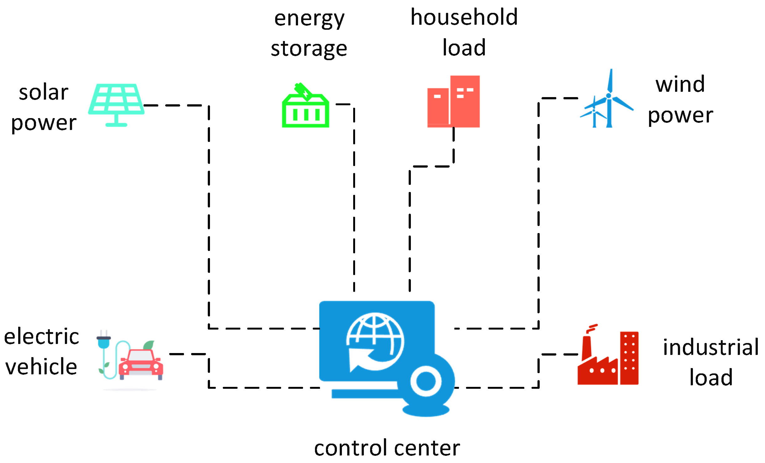
VPPs serve as a way to realize the aggregation and coordinated optimization of distributed energy resources such as distributed power sources, energy storage systems, controllable loads, electric vehicles, and other distributed energy resources through advanced information and communication technologies and software systems. The general structure of a VPP is shown in Figure 1, and this paper focuses on a typical VPP that integrates a combination of wind energy, energy storage, and electric vehicles to participate in the frequency regulation of the power system.

Figure 1.
General structure of VPP.
2.2. Wind Storage System Frequency Modulation Model
The expression for the general wind turbine aerodynamic system is shown in [23]. Under the condition of constant wind speed and maintaining the optimal tip speed ratio, the adjustment of the output power of the wind turbine is realized by changing the size of the pitch angle opening. Now, consider the following wind turbine model:
where is the angular change in paddle pitch angle, is the wind turbine power transfer function, is the wind turbine response time, and is the pitch angle control slope.
The long response time of the pitch angle of the wind turbine leads to a reduction in the frequency modulation capability, and it is necessary to combine the energy storage system with fast response capability to suppress the power fluctuation. The energy storage model of the VPP can be represented as follows [24]:
where is the storage instantaneous power, is the storage system transfer function, and is the storage system response time.
2.3. Electric Vehicle Frequency Modulation Model
As a flexible control resource, the charging and discharging processes of electric vehicles can be regarded as load and power supply, respectively, for the power grid. With the number of cars fixed, consider the following frequency modulation model for electric vehicles [25]:
where represents the depth of charge and discharge of the electric vehicle battery, and is the electric vehicle system response time.
2.4. Distributed Predictive LFC Model with VPP
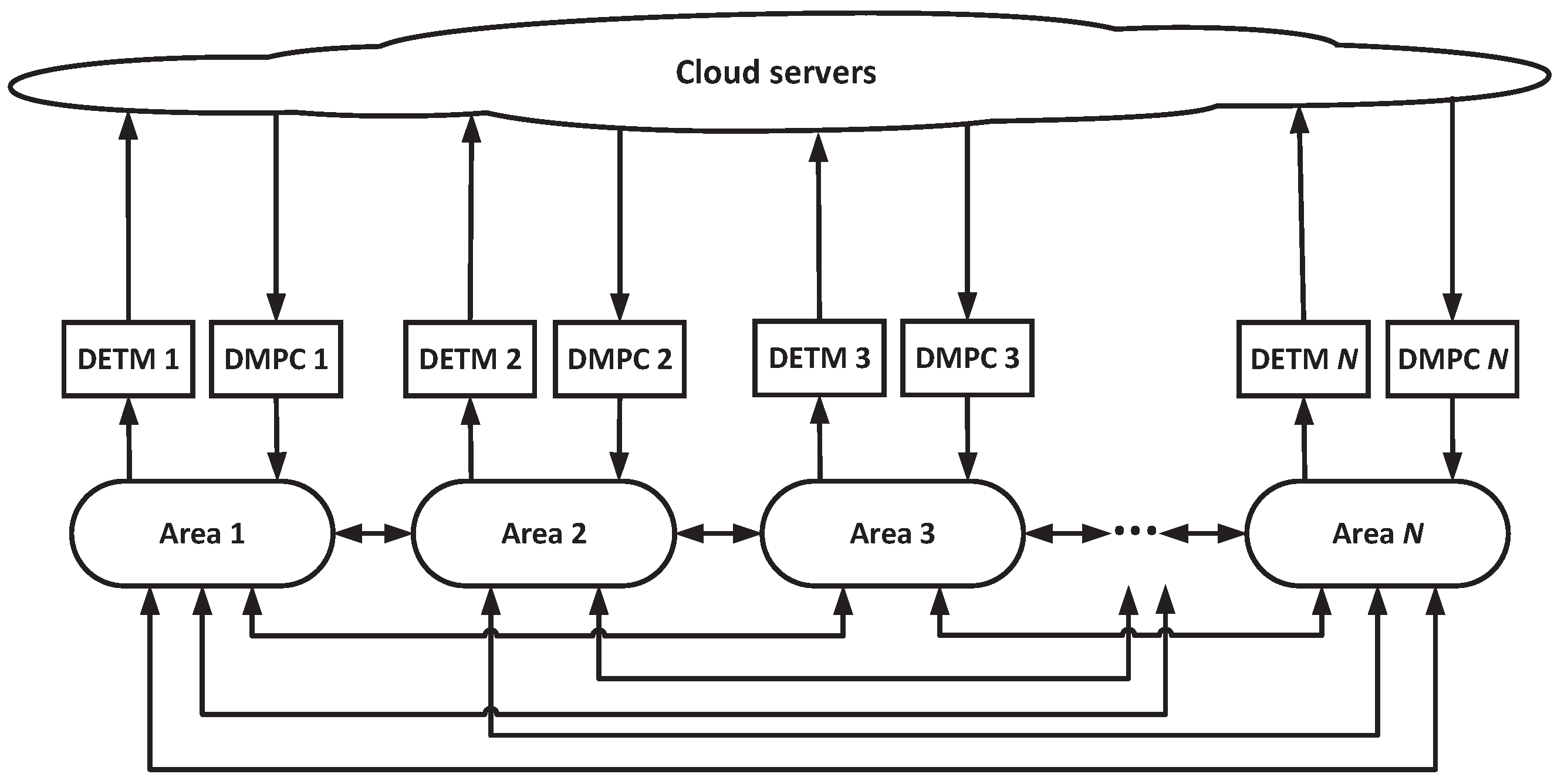
In Figure 2, we give the system structure and consider the following dynamic model of LFC with VPP for the ith control area:
where
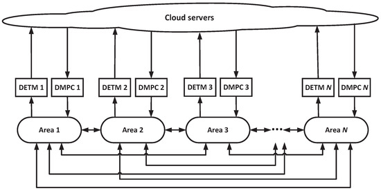
Figure 2.
Structure of multiple VPPs using DETM-based DMPC under loud–edge–terminal framework.
For explanations regarding the parameters in Equation (4), please refer to [3] for details.
The discrete-time model of LFC for a VPP for the ith control area is given as follows:
where , , , , , and are the discretized coefficient matrices.
Remark 1.
In Figure 2, each control area contains distributed energy from wind energy, energy storage, and vehicle clusters in the VPP. The distributed model predictive controllers are designed for the edge servers of each VPP, which reduces the processing time of the data and the communication delay. In addition, each control area is a terminal, and the cloud server is used for uploading and downloading data. Under this cloud–edge–terminal framework, DETMs are utilized to manage the release of packets, thereby reducing network congestion and achieving low-delay communication.
Suppose that the load disturbance satisfies
where is constant.
Consider the following hard constraints:
where the vector is given with its elements being nonnegative.
To reduce communication delay and increase the packet transmission rate, the following DETM is presented:
where stands for the mth instant for data release, is a dynamic variable (DV) with , is an adaptive adjustment variable (AAV), is a weighting matrix, , , , and are given constants, and where .
Note that in DETM (8), there exist a DV and an AAV , which are incorporated to enhance the capability of adjusting releases of data packets. Additionally, we have
Let
Then, we obtain
which holds for any .
Remark 2.
In (8), a new DETM is designed that contains an AVV with adjustable upper and lower bounds to flexibly regulate packet releases. In addition, DETM (8) can also be degraded to existing DETMs by setting suitable parameters. For example, by setting , , , , , and , DETM (8) becomes the DETM in [13]. As a result, DETM (8) is more general and flexible than existing DETMs, which can further decrease the possibility of network congestion and thus reduce communication delay.
To further reduce the communication delay, a distributed control strategy is used to shorten the data processing time. A distributed state feedback controller for the ith control area can be designed:
The state feedback controller of the neighboring subsystem is expressed as
For ease of presentation, we define
The following prediction model is given:
Consider the following objective function:
where , , , and are given weighting matrices, and is a constant.
For DMPC in each area i, and at each time instant k, we construct the following “min=-max” optimization problem (OP) to design the DMPC controllers for System (14):
where
where and give the weighting matrix to be designed and the optimisation index, respectively.
Definition 1.
For System (5), the set is a positively invariant set (PIS) if , .
Lemma 1.
In DETM (8), where , if the constants , , , , , and satisfy and , then .
Proof.
It is not difficult to complete the proof by following the method in [14]; the details are thus omitted. □
Since it is difficult to solve directly, we need to transform . Therefore, we next propose an LMI-based auxiliary OP for and then develop a DETM-based DMPC algorithm to design the controller gain matrix and the DETM weighting matrix .
3. Main Results
3.1. LMI-Based Auxiliary of
In this section, we will design a DMPC algorithm based on the DETM (8) for System (14). To achieve this goal, we design an LMI-based auxiliary OP to solve .
Consider the following Lyapunov-like function:
At each time instant k, we suppose the following inequality:
Adding both sides of (21) from to , we obtain
Based on (23), we construct the following auxiliary OP:
Theorem 1.
Let the scalars , , , , and , and the matrices and be given. If a scalar and matrices , , , , and exist such that, , the following LMIs
hold, where
then conditions (17a) and (21) are satisfied, and the feedback gain matrix and the weighting matrix are designed by
Proof.
It follows from (15) that
Further, we obtain
where
Pre- and post-multiply the left-hand side matrix of Inequality (34) by diag and its transpose, respectively. Then, by denoting and (28), we have
where
Then, (17a) holds if there exists a matrix such that
and (27) are met.
By the Schur complement, we obtain
3.2. Sufficient Conditions for PIS
To ensure that is a PIS, we give sufficient conditions and give the corresponding LMIs.
Theorem 2.
Define the scalar satisfying , and the scalars associated with DETM (8) are the same as in Theorem 1. If there exist a scalar and matrices , , , and such that the LMIs
Proof.
Noting that , by Schur complement, we know that (39) guarantees ; further, we obtain . Due to the presence of disturbance, we need to prove that .
The invariant set (18) holds at if
Substituting (6) into (41), and noting that , we have that , and thus . This proves that . Furthermore, we obtain that (41) is ensured by (40) [the detailed proof is similar to the proof of Theorem 1 and is omitted here]. Finally, the condition (17b) is guaranteed by (39) and (40). This completes the proof. □
From the sufficient conditions given above, we transform into the following auxiliary OP:
Based on , we give Algorithm 1.
| Algorithm 1 DETM-based DMPC for System (14) |
Step 1. At , set the initial state , the matrices and , and set the scalars , , , , , , , , , , , and . Step 2. If the error between and meets the event-triggered condition in DETM (8), then update by ; otherwise, implement on the controller. |
4. Case Study
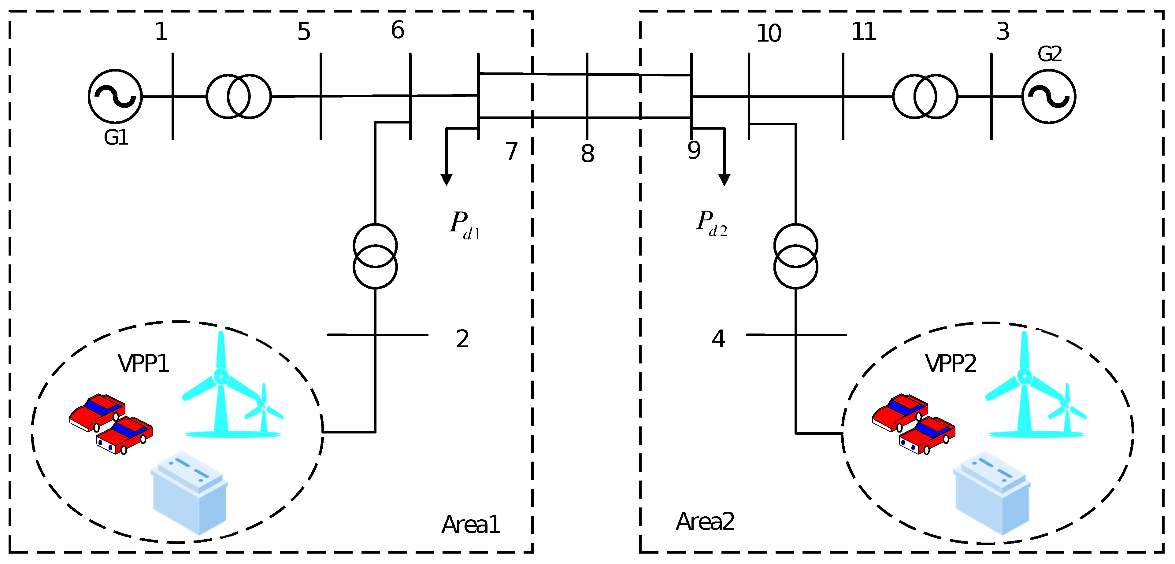
To illustrate the superiority of our proposed approach, we construct the model of an 11-node LFC system in two areas, as shown in Figure 3. Areas 1 and 2 include 600 MW thermal power units, G1 and G2, respectively, and each area contains a VPP aggregating wind power, energy storage, and electric vehicles. In each area, all generation units are simplified as an equivalent generation unit, and the system parameters (see Table 1 and Table 2) are borrowed from [26].
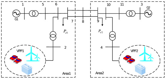
Figure 3.
System simulation.

Table 1.
Parameters of two-area power system.
Table 2.
Parameters of two virtual power plants.
Let , and the scalars , , , , , , , , , , , , and , and the matrices and . Set and . Select the discretization period .
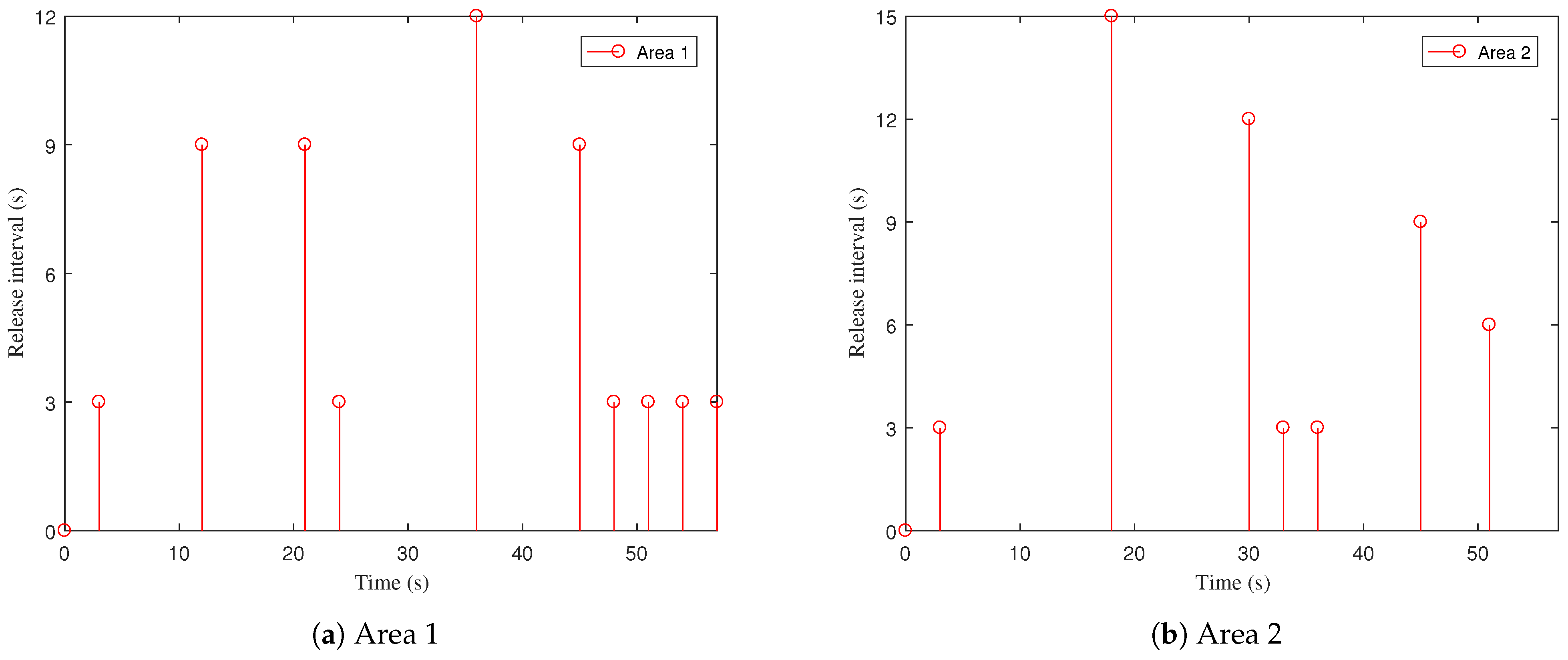
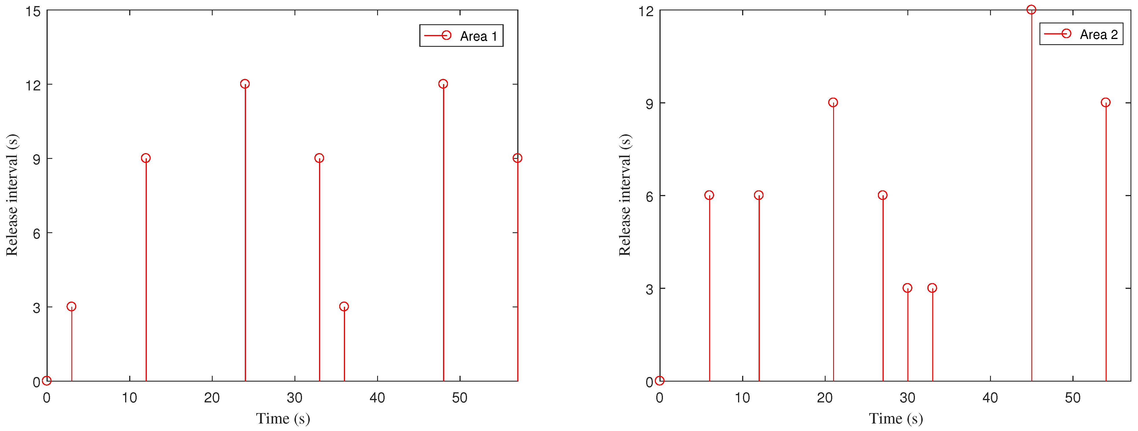
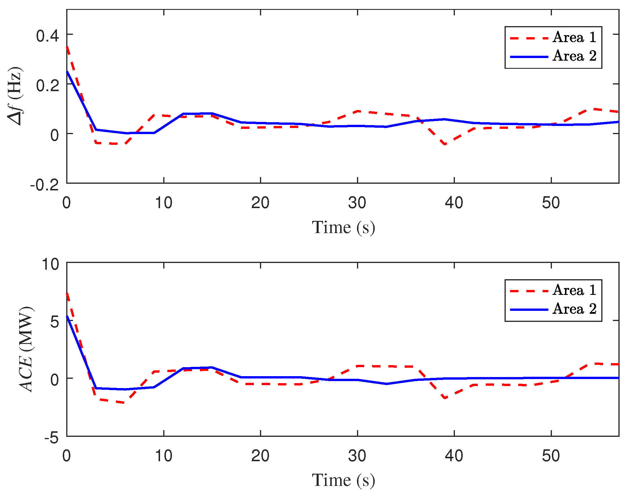
Scenario 1. Suppose that in the first 60 s, there exist step load disturbances with and .
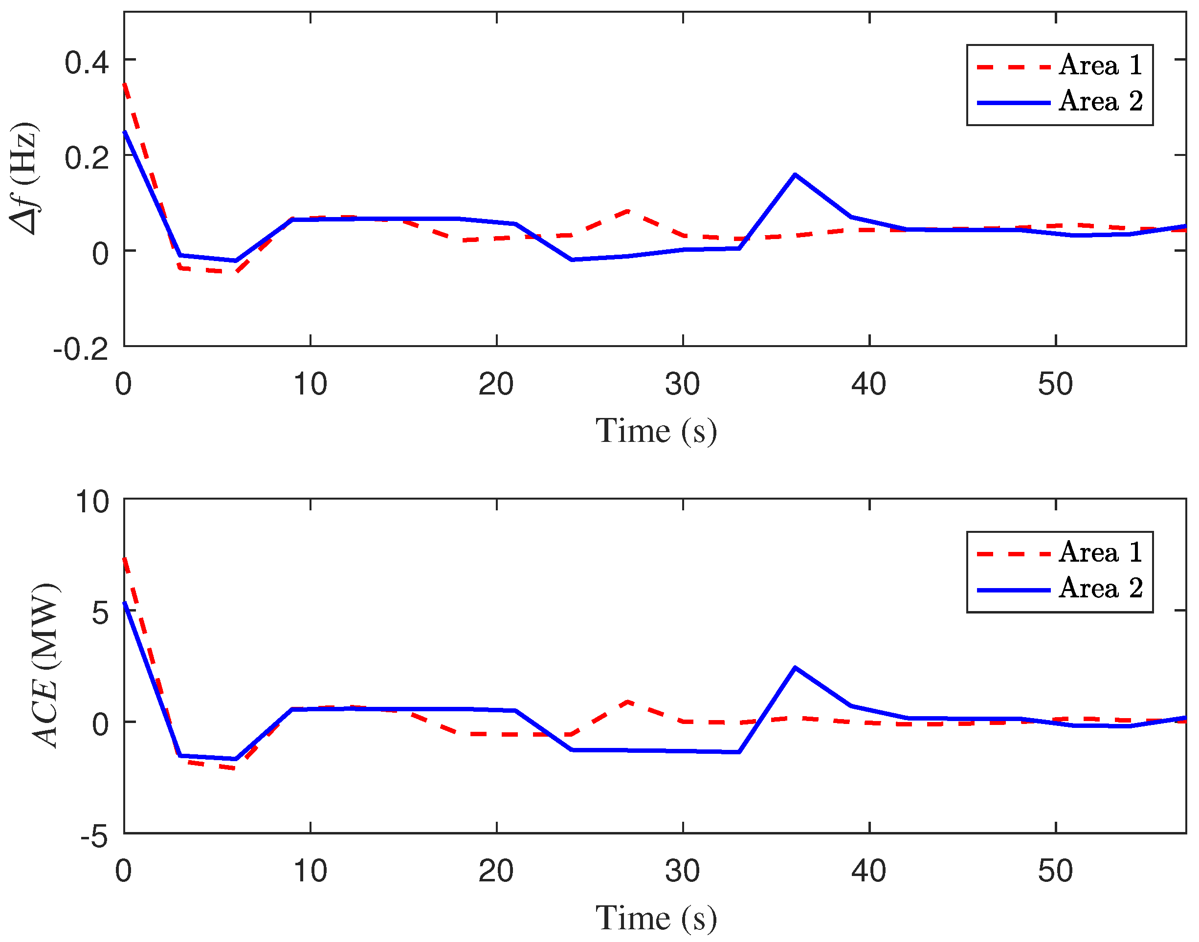
Figure 4 shows the DETM triggering instants and release intervals for Area 1 (Area 2). Figure 5 shows the trajectories of and . The above simulation results indicate that the designed dynamic event-based DMPC algorithm is able to reduce packet releases while achieving control performance, thus reducing the communication delay of the VPP.
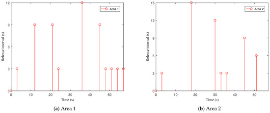
Figure 4.
DETM evolutions of two areas under step load disturbances.
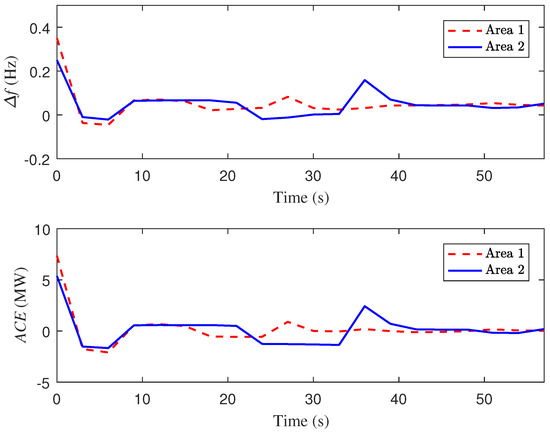
Figure 5.
Trajectories of and subjected to step load disturbances.
To further illustrate the superiority of DETM (8), we compare it with DETM in [13]. By setting , , , , , and and keeping the other parameters of DETM (8), we can obtain DETM in [13].
Table 3 gives the average triggering rates (ATRs) of the above two DETMs for two areas, and it can be noticed that the ATR of DETM (8) is lower than that of DETM in [13]. This means that the DMPC algorithm under DETM (8) is able to significantly reduce the ATR, thus reducing network congestion and decreasing the communication delay of the VPP at a slight sacrifice of control performance (see Table 4 for the detailed performance comparison of different algorithms, where summation of the absolute value of the error (SAE), summation of the square value of the error (SSE), and summation of the time multiplied by square value of the error (STSE) are defined as , , and with and ).
Table 3.
ATRs under DETM (8) and DETM in [13] for the case of step load disturbances.
Table 4.
Performance comparison under step load disturbances between different algorithms.
In Table 5, we list the data processing time under DMPC and CMPC algorithms on the MATLAB R2016b platform with Intel(R) Core(TM) i5-8300H CPU @2.3 GHz. We obtain from Table 4 and Table 5 that, under the cloud-edge-terminal framework, compared with the CMPC algorithm under DETM (8), the DMPC algorithm under DETM (8) is able to shorten the data processing time while guaranteeing the control performance. The above results demonstrate that the DMPC algorithm under DETM (8) reduces the network burden and shortens the data processing time, which helps to reduce the communication delay of the VPP.
Table 5.
Data processing time under DMPC and CMPC algorithms.
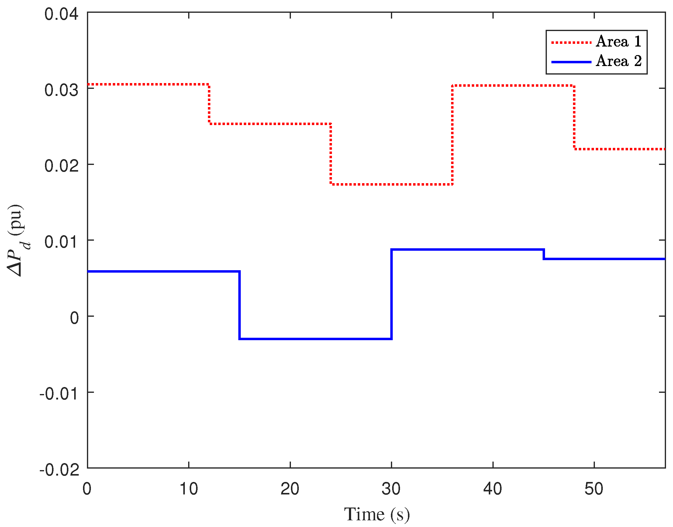
Scenario 2. Suppose that in the first 60 s, there exist random load disturbances, which are shown in Figure 6.

Figure 6.
Random load disturbances.
Figure 7 shows the DETM triggering instants and release intervals for Area 1 (Area 2). Figure 8 gives the trajectories of and . The above results show that the dynamic event-based DMPC algorithm reduces the packet releases and the communication delay of the VPP while achieving the desired control performance.
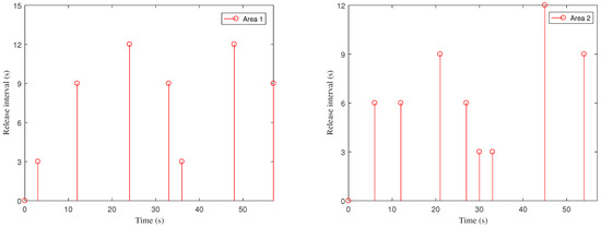
Figure 7.
DETM evolutions of two areas under random load disturbances.
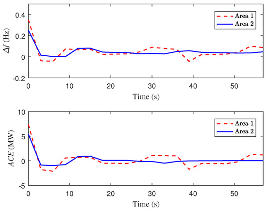
Figure 8.
Trajectories of and subjected to random load disturbances.
To further illustrate that our proposed algorithm is also superior under random load disturbances, we compare the DMPC algorithms under DETM (8) and DETM in [13]. The corresponding ATRs for the above two DETMs are shown in Table 6, from which we can observe that the ATR of DETM (8) is lower than that of DETM in [13]. In other words, the DMPC algorithm under DETM (7) can significantly reduce the ATR at a slight sacrifice of control performance (see Table 6 for the detailed performance comparison of different algorithms). Therefore, the DMPC algorithm under DETM (8) is able to reduce the release of packets and thus decrease the communication delay of the VPP.
Table 6.
ATRs under DETM (8) and DETM in [13] for the case of random load disturbances.
In addition, under the cloud–edge–terminal framework, we give the performance criteria of the DMPC algorithm and CMPC algorithm under random load disturbances in Table 7, and the result shows that the DMPC algorithm under DETM (8) can guarantee the control performance. The data processing time under the two MPC algorithms is almost identical to the corresponding results in Table 5 and is thus omitted here. The above experimental results show that the DMPC algorithm under DETM (8) can shorten the data processing time while guaranteeing the control performance, which contributes to a reduction in the communication delay of the VPP.
Table 7.
Performance comparison under random load disturbances between different algorithms.
5. Conclusions
The DETM-based distributed model predictive LFC problem is investigated for VPPs under the cloud-edge-terminal framework. We design a new DETM that manages packet release more flexibly than several existing ETMs and reduces network congestion, which further reduces the communication delay of the VPP. Based on the above DETM, we design DMPC controllers for each edge server of the VPP. Specifically, to facilitate the solution of the “min-max” OP of the DMPC, we design an auxiliary OP which utilizes the Lyapunov-like function containing a DV, and then transform it into another auxiliary OP with LMI constraints which provides the design method of the DMPC controller. A case study of two-area VPPs is given to illustrate the effectiveness and superiority of the DETM-based DMPC approach under the cloud-edge-terminal framework. The designed DETM-based DMPC algorithm is able to save network resources and shorten data processing time while maintaining the control performance, which helps to reduce the communication delay of the VPP.
Author Contributions
Conceptualization, K.K. and N.S.; methodology, K.K., N.S., and S.C.; validation, L.Z., X.S., and H.C.; formal analysis, K.K., N.S., and M.F.; investigation, K.K., S.C., S.Z., and X.W.; writing—original draft preparation, L.Z., X.S., and H.C.; writing—review and editing, M.F., S.Z., X.W., and K.K. All authors have read and agreed to the published version of the manuscript.
Funding
This research was supported by the project “Research and Applications of Key Technology for Virtual Power Plants in New Power Systems Subject to Cloud-Edge-Terminal Collaboration and Source-Grid-Load-Storage Integration” from PowerChina Hubei Electric Engineering Co., Ltd. (Project Number: DJ-ZDXM-2023-14).
Data Availability Statement
The data is contained within the article.
Conflicts of Interest
Author Kai Kang is employed by the company PowerChina Hubei Engineering Co., Ltd., Authors Nian Shi, Si Cai, Liang Zhang, Xinan Shao, Haohao Cao, Mingjin Fei are employed by the company PowerChina Hubei Electric Engineering Co., Ltd. The remaining authors declare that the research was conducted in the absence of any commercial or financial relationships that could be construed as a potential conflict of interest.
Abbreviations
The following abbreviations are used in this manuscript:
| VPP | virtual power plant |
| LFC | load frequency control |
| DMPC | distributed model predictive control |
| CMPC | centralized model predictive control |
| DETM | dynamic event-triggered mechanism |
| OP | optimization problem |
| DV | dynamic variable |
| AAV | adaptive adjustment variable |
References
- Zhang, Y.; Shi, X.; Zhang, H.; Cao, Y.; Terzija, V. Review on deep learning applications in frequency analysis and control of modern power system. Int. J. Electr. Power Energy Syst. 2022, 136, 107744. [Google Scholar] [CrossRef]
- Lan, Y.; Illindala, M.S. Robust distributed load frequency control for multi-area power systems with photovoltaic and battery energy storage system. Energies 2024, 17, 5536. [Google Scholar] [CrossRef]
- Shangguan, X.C.; Zhang, C.K.; He, Y.; Jin, L.; Jiang, L.; Spencer, J.W.; Wu, M. Robust load frequency control for power system considering transmission delay and sampling period. IEEE Trans. Ind. Inform. 2022, 17, 5292–5303. [Google Scholar] [CrossRef]
- Chen, X.; Qu, G.; Tang, Y.; Low, S.; Li, N. Reinforcement learning for selective key applications in power systems: Recent advances and future challenges. IEEE Trans. Smart Grid 2022, 13, 2935–2958. [Google Scholar] [CrossRef]
- Chen, J.; Liu, M.; Milano, F. Aggregated model of virtual power plants for transient frequency and voltage stability analysis. IEEE Trans. Power Syst. 2021, 36, 4366–4375. [Google Scholar] [CrossRef]
- Wang, Z.; Wang, Y.; Xie, L.; Pang, D.; Shi, H.; Zheng, H. Load frequency control of multiarea power systems with virtual power plants. Energies 2024, 17, 3687. [Google Scholar] [CrossRef]
- Li, X.; Li, C.; Liu, X.; Chen, G.; Dong, Z.Y. Two-stage community energy trading under end-edge-cloud orchestration. IEEE Internet Things J. 2023, 10, 1961–1972. [Google Scholar] [CrossRef]
- Lin, W.T.; Chen, G.; Zhou, X. Distributed carbon-aware energy trading of virtual power plant under denial of service attacks: A passivity-based neurodynamic approach. Energy 2022, 257, 124751. [Google Scholar] [CrossRef]
- Hu, G.; Zhu, Y.; Zhao, D.; Zhao, M.; Hao, J. Event-triggered communication network with limited-bandwidth constraint for multi-agent reinforcement learning. IEEE Trans. Neural Netw. Learn. Syst. 2023, 34, 3966–3978. [Google Scholar] [CrossRef]
- Bu, X.; Yu, W.; Cui, L.; Hou, Z.; Chen, Z. Event-triggered data-driven load frequency control for multiarea power systems. IEEE Trans. Ind. Inform. 2022, 18, 5982–5991. [Google Scholar] [CrossRef]
- Wang, M.; Cheng, P.; Zhang, Z.; Wang, M.; Chen, J. Periodic event-eriggered MPC for continuous-time nonlinear systems with bounded disturbances. IEEE Trans. Autom. Control 2023, 68, 8036–8043. [Google Scholar] [CrossRef]
- Wan, X.; Wei, F.; Zhang, C.K.; Wu, M. Networked output-feedback MPC: A bounded dynamic variable and time-varying threshold-dependent event-based approach. IEEE Trans. Cybern. 2024, 54, 2308–2319. [Google Scholar] [CrossRef] [PubMed]
- Shi, T.; Shi, P.; Chambers, J. Dynamic event-triggered model predictive control under channel fading and denial-of-service attacks. IEEE Trans. Autom. Sci. Eng. 2024, 21, 6448–6459. [Google Scholar] [CrossRef]
- Wan, X.; Han, T.; An, J.; Wu, M. Fault diagnosis for networked switched systems: An improved dynamic event-based scheme. IEEE Trans. Cybern. 2022, 52, 8376–8387. [Google Scholar] [CrossRef]
- Zhang, M.; Dong, S.; Shi, P.; Chen, G.; Guan, X. Distributed observer-based event-triggered load frequency control of multiarea power systems under cyber attacks. IEEE Trans. Autom. Sci. Eng. 2023, 20, 2435–2444. [Google Scholar] [CrossRef]
- Fang, X.; Xu, M.; Fan, Y. SOC-SOH estimation and balance control based on event-triggered distributed optimal kalman consensus filter. Energies 2024, 17, 639. [Google Scholar] [CrossRef]
- Shen, H.; Wang, D.; Park, J.H.; Sreeram, V.; Wang, J. Switching-like event-triggered sliding mode load frequency control for networked power systems under energy-limited DoS attacks. IEEE Trans. Syst. Man Cybern. Syst. 2024, 54, 1589–1598. [Google Scholar] [CrossRef]
- Yang, Q.; Chen, G.; Guo, M.; Chen, T.; Luo, L.; Sun, L. Model predictive hybrid PID control and energy-saving performance analysis of supercritical unit. Energies 2024, 17, 6356. [Google Scholar] [CrossRef]
- Zhang, B.; Song, Y. Model-predictive control for Markovian jump systems under asynchronous scenario: An optimizing prediction dynamics approach. IEEE Trans. Autom. Control 2022, 67, 4900–4907. [Google Scholar] [CrossRef]
- Tang, X.; Li, Y.; Yang, M.; Wu, Y.; Wen, Y. Adaptive event-triggered model predictive load frequency control for power systems. IEEE Trans. Power Syst. 2023, 38, 4003–4014. [Google Scholar] [CrossRef]
- Bolzoni, A.; Parisio, A.; Todd, R.; Forsyth, A.J. Optimal virtual power plant management for multiple grid support services. IEEE Trans. Energy Convers. 2021, 36, 1479–1490. [Google Scholar] [CrossRef]
- Bao, P.; Zhang, W.; Zhang, Y. Secondary frequency control considering optimized power support from virtual power plant containing aluminum smelter loads through VSC-HVDC link. J. Mod. Power Syst. Clean Energy 2023, 11, 355–367. [Google Scholar] [CrossRef]
- Wang, C.; Liu, X.; Lee, K.Y. Two-layer robust distributed predictive control for load frequency control of a power system under wind power fluctuation. Energies 2023, 16, 4714. [Google Scholar] [CrossRef]
- Ma, Y.; Hu, Z.; Song, Y. A Reinforcement learning based coordinated but differentiated load frequency control method with heterogeneous frequency regulation resources. IEEE Trans. Power Syst. 2024, 39, 2239–2250. [Google Scholar] [CrossRef]
- Qiao, S.; Liu, X.; Wang, Y.; Xiao, G.; Wang, P. H∞ load frequency control of power system integrated with EVs under DoS attacks: Non-fragile output sliding mode control approach. IEEE Trans. Intell. Transp. Syst. 2024, 25, 4565–4577. [Google Scholar] [CrossRef]
- Peng, C.; Zhang, J.; Yan, H. Adaptive event-triggering H∞ load frequency control for network-based power systems. IEEE Trans. Ind. Electron. 2018, 65, 1685–1694. [Google Scholar] [CrossRef]
Disclaimer/Publisher’s Note: The statements, opinions and data contained in all publications are solely those of the individual author(s) and contributor(s) and not of MDPI and/or the editor(s). MDPI and/or the editor(s) disclaim responsibility for any injury to people or property resulting from any ideas, methods, instructions or products referred to in the content. |
© 2025 by the authors. Licensee MDPI, Basel, Switzerland. This article is an open access article distributed under the terms and conditions of the Creative Commons Attribution (CC BY) license (https://creativecommons.org/licenses/by/4.0/).