Integrating Kolmogorov–Arnold Networks with Time Series Prediction Framework in Electricity Demand Forecasting

Abstract

Electricity demand is driven by a diverse set of factors, including fluctuations in business cycles, interregional dynamics, and the effects of climate change. Accurately quantifying the impact of these factors remains challenging, as existing methods often fail to address the complexities inherent in these influences. This study introduces a time series forecasting model based on Kolmogorov–Arnold Networks (KANs), integrated with three advanced neural network architectures, Temporal Convolutional Network (TCN), Bidirectional Long Short-Term Memory (BiLSTM), and Transformer, to forecast UK electricity demand. The analysis utilizes real-world datasets from a leading utility company and publicly available sources. Experimental findings reveal that the integration of KANs significantly improves forecasting accuracy, robustness, and adaptability, particularly in modeling intricate sequential patterns in electricity demand time series. The proposed approach addresses the limitations of traditional time series models, underscoring the potential of KANs as a transformative tool for predictive analytics.

1. Introduction

Electricity demand forecasting plays a critical role in modern energy management. With the increasing strain on energy resources, enhancing forecasting accuracy through advanced models is essential for optimizing energy allocation and utilization. This is not only pivotal for the advancement of the power industry but also provides indispensable technical support for addressing global energy challenges. Numerous methods have been developed for electricity demand forecasting, ranging from traditional statistical techniques, such as regression analysis and autoregressive models, to more advanced approaches. Traditional methods, which rely on historical data, are well-suited for short-term and medium-term forecasting [1], but they exhibit significant limitations in long-term predictions. Statistical approaches such as ARIMA, ETS, and Prophet effectively address seasonality, long-term trends, and noise; however, their reliance on linearity assumptions, extensive historical data requirements, and restricted capacity to model complex non-linear relationships hinder their adaptability to abrupt structural changes in the data [2]. In contrast, machine learning models, such as support vector machines (SVMs) and artificial neural networks (ANNs), have been extensively employed for forecasting monthly electricity demand across different countries and regions [3]. While these models demonstrate strong nonlinear modeling capabilities, they are often susceptible to overfitting and struggle to effectively capture long-term trends. Grey prediction models, although capable of enhancing forecasting accuracy through data sequence transformation and background value optimization, are constrained by their sensitivity to initial conditions and reliance on small sample sizes. These limitations make it difficult for grey models to manage highly volatile or complex datasets effectively [4]. Although machine learning techniques are widely utilized in electricity demand forecasting [5,6,7,8,9,10,11], their inherent shortcomings have motivated researchers to explore alternative approaches.

Time series forecasting plays a vital role in various fields, influencing key decision-making processes in finance, medicine, economics, biology, and meteorology, highlighting its broad applicability and significance across disciplines [12,13,14,15]. In recent years, the application of time series models to forecast trends, seasonal variations, and cyclical patterns in electricity demand has garnered significant interest [16,17,18,19,20]. Ahmed et al. [21] addressed the complex multi-source power load forecasting problem by employing an ensemble learning method, integrating multiple predictive factors into the model, and achieving high prediction accuracy. Shi et al. [22] proposed a deep neural network model based on long short-term memory (LSTM) and recurrent neural networks (RNNs) for short-term electricity demand forecasting, although factors such as weather were not considered. To enhance forecasting performance, techniques such as optimization algorithms, integration methods, and time series decomposition have emerged as key technologies [23]. Kenneth [24] examined terminal energy consumption in Canada, the Asia-Pacific region, the United States, and European countries, incorporating socio-economic development factors. The findings revealed a nonlinear growth relationship between per capita income and electricity consumption. Similarly, Jovanovic [25] identified national-level factors, such as economic governance and population size, as critical determinants of electricity demand alongside economic variables.

Building on advancements in time series forecasting and the identification of key determinants of electricity consumption, this study seeks to improve the accuracy and reliability of electricity demand predictions by integrating Kolmogorov–Arnold Networks (KANs) with three established time series models: Transformer, Bidirectional Long Short-Term Memory (BiLSTM), and Temporal Convolutional Network (TCN).

The Transformer model, celebrated for its ability to capture long-range dependencies through self-attention mechanisms, offers substantial advantages in modeling intricate temporal relationships [26,27]. However, optimizing sparse attention for diverse data structures remains a challenge, as it may lead to the loss of critical information in highly dynamic sequences [28]. Long Short-Term Memory (LSTM) and its bidirectional variant, BiLSTM, are widely utilized for their proficiency in capturing long-term dependencies within sequential data [29]. BiLSTM extends this capability by processing input sequences in both forward and backward directions, enabling it to capture dependencies spanning past to present as well as present to future. This dual processing enhances prediction accuracy, often outperforming unidirectional LSTM in tasks such as stock price prediction [30]. TCN is another powerful deep learning architecture specifically designed for time series data, excelling at capturing local dependencies through convolutional operations. TCNs are highly adaptable and have been effectively applied to various forecasting tasks, including weather prediction [31] and short-term load forecasting for industrial users [32]. However, the increased complexity of BiLSTM and TCN makes them more prone to overfitting, especially when trained on smaller datasets, and they typically require larger amounts of data to achieve optimal performance [33].

Recent studies have introduced Kolmogorov–Arnold Networks (KANs) [34] as an innovative neural network architecture grounded in the Kolmogorov–Arnold representation theorem [35,36]. This theorem asserts that any multivariate continuous function can be expressed as a composition of univariate functions and addition operations. This foundational principle sets KANs apart from traditional Multi-Layer Perceptrons (MLPs) [37]. By leveraging the representation theorem [38], KANs enhance both accuracy and interpretability, enabling them to achieve comparable or even superior performance with more compact architectures in tasks such as data fitting and solving partial differential equations. Kolmogorov–Arnold Networks (KANs) have gained significant attention as a promising method in electrical engineering. For instance, Cabral et al. [39] utilized KANs for fault diagnosis in oil-immersed power transformers, highlighting their reliability in handling real-world imbalanced datasets. Jiang et al. [40] proposed the D_KAN model, integrating KANs with DLinear to enhance power load forecasting through improved accuracy and adaptability. Shuai et al. [41] developed physics-informed KANs for dynamic modeling of power systems, showcasing their ability to integrate physical constraints into data-driven models for improved interpretability. Dao et al. [42] employed KANs for estimating the state of charge in lithium-ion batteries and demonstrated that KANs provide more accurate predictions in complex scenarios. These studies highlight the significant potential of KANs in advancing electrical engineering applications.

To achieve more accurate power demand forecasting, this study integrates KAN with three established models. By utilizing these methods, the complex relationships and nonlinearities inherent in power demand are effectively captured, enabling a more comprehensive and precise analysis of the factors influencing power demand.

This paper is organized as follows. Section 2 outlines the materials and methods, detailing the data collection, preprocessing techniques, and feature selection process for power demand forecasting. Section 3 provides the theoretical background, covering time series models and the Kolmogorov–Arnold representation theorem, while also explaining the experimental framework and process. Section 4 presents the forecasting results and evaluates the performance of KAN integrated with time series models. Finally, Section 5 summarizes the study’s contributions and discusses potential future research directions.

2. Materials and Methods

In order to establish a UK electricity demand forecasting model, this study collected monthly electricity consumption data, along with various related datasets, from 2015 to April 2024 (

Table 1. Factor types and descriptions and importance.

Factors	Description	Pearson Coefficient	Mutual Information
National demand—nd	National demand is the sum of metered generation	1	-
Electricity consumption—x2	Monthly electricity consumption from users in the UK	0.98	0.83
England electricity generation—x3	Monthly electricity generation in England	0.86	0.94
Wales electricity generation—x4	Monthly electricity generation in Wales	0.56	1.06
Regional Total precipitation—x5	Monthly measures of regional total precipitation	0.43	0.58
Regional average temperature—x6	Monthly measures of regional average temperature	0.40	0.60
Regional average wind speed—x7	Monthly measures of regional average wind speed	0.35	0.42
Regional economy—x8	Monthly CPI in a region	−0.13	0.21
Transmission system demand—x9	Monthly measures of transmission system demand additional generation required to meet station load, pump storage pumping, and interconnector exports	0.11	0.28

). These datasets include, but are not limited to, economic and meteorological data. In this analysis, the total electricity demand in the UK (national demand, nd) is modeled as the dependent variable. The collected monthly data are time-series data, some of which exhibit a certain periodicity over time and include eight distinct factors (Figure 1).

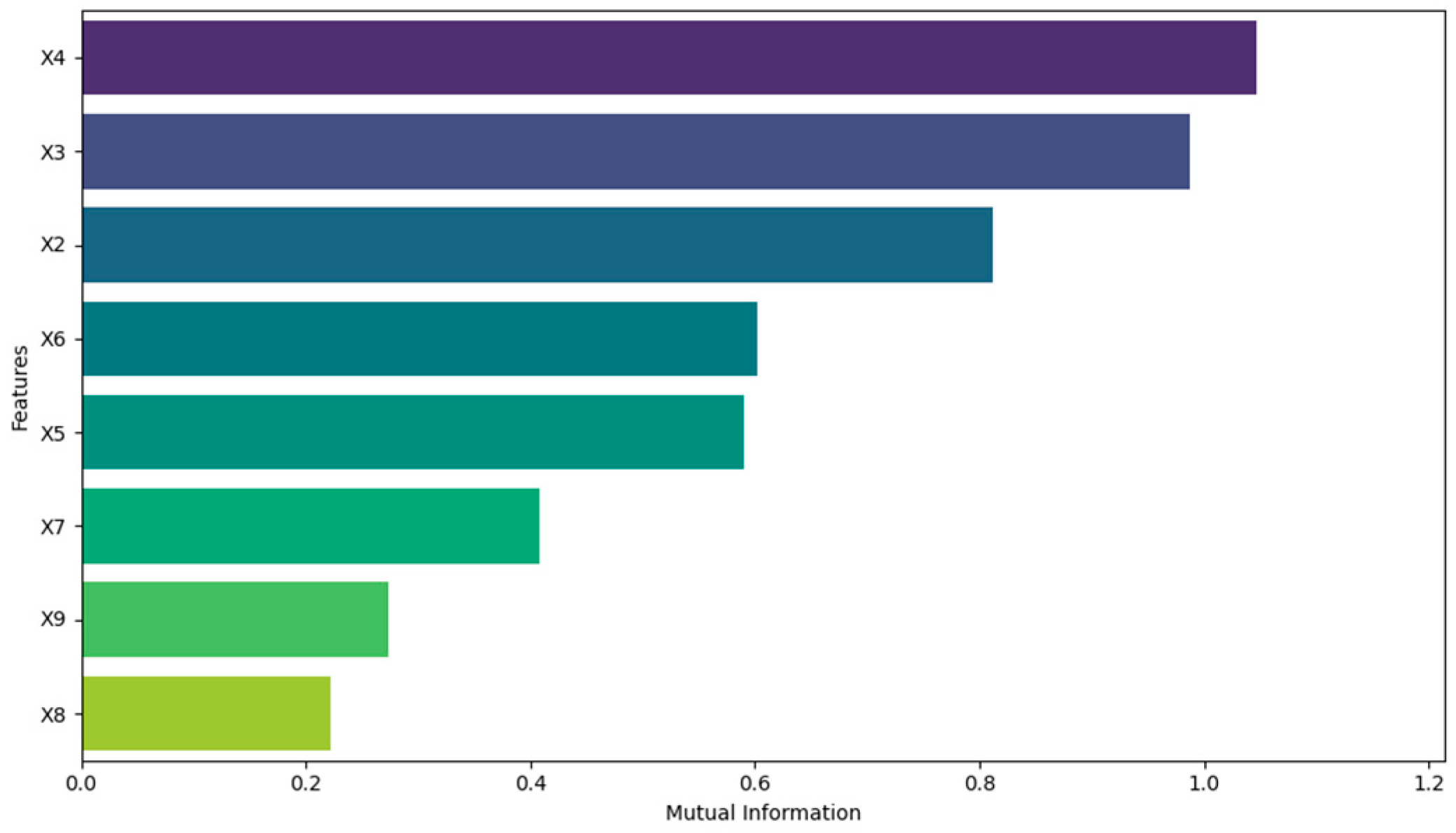
Electricity demand in the UK is influenced by a variety of economic, environmental, and regional factors. Industrial electricity consumption (x2) is a significant component of total electricity demand, reflecting the monthly consumption of users nationwide. According to the UK’s regional electricity mobility policy, England and Wales exhibit relatively concentrated patterns of electricity production and consumption. The majority of the electricity supply in these regions is managed and distributed through a unified power transmission network, resulting in a strong relationship between regional power generation (e.g., England x3, Wales x4) and electricity consumption. Meteorological factors, including precipitation (x5), temperature (x6), wind speed (x7), and others, are key variables that influence electricity demand. Particularly during cold winters and hot summers, temperature fluctuations significantly affect both household and industrial electricity demand. Wind speed and precipitation may further influence electricity consumption by affecting climate comfort and the frequency of air conditioning and heating system use. Furthermore, the Consumer Price Index (CPI, x8), as an economic variable, may negatively impact electricity demand. Research indicates that when the CPI rises [43,44], higher consumer goods prices typically reduce purchasing power, thereby decreasing electricity demand. Transmission system demand (x9) is another critical factor, representing the additional generation needed to accommodate regional load changes or demand fluctuations via inter-regional electricity transmission. By analyzing the Pearson correlation coefficient heat map (Figure 2) and mutual information plot (Figure 3) of these factors, the relationship between each variable and nation demand can be quantified. The Pearson coefficient and mutual information are shown in Table 1.

3. Theory and Calculation

3.1. KANs Background

Kolmogorov–Arnold Networks (KANs) [34] represent a novel neural network architecture inspired by the Kolmogorov–Arnold representation theorem, designed to serve as an alternative to traditional Multi-Layer Perceptrons (MLPs). The Kolmogorov–Arnold representation theorem [35] posits that any multivariate continuous function f that depends on $x=\left[x_1,x_2,\dots ,x_n\right]$ within a bounded domain can be represented as a finite composition of simpler continuous functions involving only one variable. Formally, a real, smooth, and continuous multivariate function $f\left(x\right):{\left[\mathrm{0,1}\right]}^n\to \mathbb{R}$ can be expressed through the superposition of univariate functions:

$$f\left(x\right)=f\left(x_1,\dots ,x_n\right)=\sum _{q=1}^{2n+1}{\mathsf{\Phi }}_q\left(\sum _{p=1}^n{\varphi }_{q,p}\left(x_p\right)\right)$$

(1)

where ${\mathsf{\varphi }}_{q,p}:\left[\mathrm{0,1}\right]\to \mathbb{R}$ is inner function, ${\mathsf{\Phi }}_q:\mathbb{R}\to \mathbb{R}$ is outer function.

The architecture of KAN is defined by a KAN layer $\mathsf{\Phi }=\left\{{\varphi }_{q,p}\right\}$, where $p=\mathrm{1,2},\dots ,n_{\mathrm{in}},q=\mathrm{1,2},\dots ,n_{\mathrm{out}}$, and the functions ${\varphi }_{q,p}$ are parameterized with learnable parameters. This structure allows KAN to capture complex nonlinear relationships in the data more effectively. A KAN with a depth of L is constructed by stacking L KAN layers, with the configuration of this deeper KAN specified by an integer array. $\left[n_0,n_1,\dots ,n_L\right]$, where $n_l$ indicates the number of neurons in the layer. Each l-th KAN layer takes an input of dimension $n_{in}$ and produces an output of dimension $n_{l+1}$, transforming the input vector $x_l\in {\mathbb{R}}^{n_l}$ to $x_{l+1}\in {\mathbb{R}}^{n_l+1}$ [34], as shown in Equation (2).

$$x_{l+1}=\underset{{\mathsf{\Phi }}_l}{\underbrace{\left(\begin{array}{cccc}{\varphi }_{l,\mathrm{1,1}}\left(\cdot \right)& {\varphi }_{l,\mathrm{1,2}}\left(\cdot \right)& ⋮& {\varphi }_{l,1,n_l}\left(\cdot \right)\\ {\varphi }_{l,\mathrm{2,1}}\left(\cdot \right)& {\varphi }_{l,\mathrm{2,2}}\left(\cdot \right)& \cdots & {\varphi }_{l,2,n_l}\left(\cdot \right)\\ ⋮& ⋮& \ddots & ⋮\\ {\varphi }_{l,n_{l+1},1}\left(\cdot \right)& {\varphi }_{l,n_{l+1},2}\left(\cdot \right)& \cdots & {\varphi }_{l,n_{l+1},n_l}\left(\cdot \right)\end{array}\right)}}$$

(2)

The function matrix ${\mathsf{\Phi }}_l$ corresponds to the l-$\mathrm{t}\mathrm{h}$ KAN layer, and the KAN is essentially formed by combining multiple KAN layers

$$KAN\left(x\right)=\left({\mathsf{\Phi }}_{L-1}\circ {\mathsf{\Phi }}_{L-2}\circ \dots \circ {\mathsf{\Phi }}_0\right)x$$

(3)

The network depth, determined by the number of layers, enables the model to capture more complex patterns and relationships within the data. Each KAN layer processes the input $x$ through a series of learnable functions ${\varphi }_{q,p}$, enabling the network to be highly adaptable and resilient.

The Kolmogorov–Arnold (KAN) representation theorem facilitates the development of novel neural network architectures by replacing conventional linear weights with univariate B-spline-based functions, which serve as learnable activation functions. These B-splines are represented through the basis functions $N_{i,j}\left(t\right)$. Integrating the network’s multilayer structure with dynamic adjustments to the activation function through a grid expansion technique allows the network to adapt to varying data resolutions. This design optimizes performance by fine-tuning the accuracy of the activation function. The flexibility of the spline enables adaptive modeling of complex relationships by reshaping the spline, minimizing approximation errors, and enhancing the network’s capability to learn intricate patterns from high-dimensional datasets. The 0th-order basis function $N_{i,0}\left(t\right)$ is defined as follows:

$$N_{i,0}\left(t\right)=\left\{\begin{array}{c}1if{t}_i\le t\le t_{i+1}and{t}_i<t_{i+1},\\ 0otherwise\end{array}\right.$$

(4)

Higher-order basis functions $N_{i,j}\left(t\right)$ are calculated using the recursive formula:

$$N_{i,j}\left(t\right)={\displaystyle \frac{t-t_i}{t_{i+j}-t_i}}{N}_{i,j-1}\left(t\right)+{\displaystyle \frac{t_{i+j+1}-t}{t_{i+j+1}-t_{i+1}}}{N}_{i+1,j-1}\left(t\right),$$

(5)

where $j=1,2,\dots ,p$, and $i$ is the index of the basis function, corresponding to the position of the first knot $t_i$ that influences $N_{i,j}\left(t\right)$, with $i=0,1,\dots ,m-j-1$, where $m$ denotes the total number of knots, ensuring the proper definition of the basis functions within the knot sequence. The B-spline curve is defined by the following equation:

$$C\left(t\right)=\sum _{i=0}^n{P}_i{N}_{i,p}\left(t\right)$$

(6)

This is called B-spline. This method provides greater adaptability in creating the architecture of the neural network and improves the KAN model’s ability to learn and represent data, allowing it to better handle nonlinear relationships within intricate datasets.

During the training process, a grid search method is used, where the parameters of the spline function (i.e., the coefficients of the basis functions) are adjusted to minimize the loss function. The shape of the spline function is dynamically refined to best fit the training data. This optimization process usually utilizes techniques such as gradient descent, and the spline function parameters are updated in each iteration to reduce the prediction error. Since KANs are similar to multi-layer perceptrons (MLPs) on the outside, they can not only extract features but also optimize features with high accuracy by leveraging their internal similarities to spline functions. KANs exhibit strong function approximation capabilities, high interpretability, smoothness, and robustness while providing flexible parameter settings and adaptive characteristics for time series forecasting. These advantages enable KANs to effectively handle a variety of complex time series data, thereby improving prediction accuracy and model stability.

3.2. BiLSTM-KANs

With its bidirectional structure, long short-term memory units, and strong context understanding capabilities, BiLSTM effectively captures long-term dependencies, thereby enhancing prediction accuracy and reliability in time series forecasting. The BiLSTM-KANs model leverages the bidirectional long short-term memory network’s ability to comprehensively capture temporal dependencies and understand the context of time series data [30]. Unlike LSTM, which typically processes information in only a forward direction, BiLSTM incorporates two layers of LSTM: one processes the input sequence in the forward direction, while the other processes it in reverse. The forward LSTM captures information about past data within the input sequence, whereas the reverse LSTM retrieves information about future data. The outputs of these two hidden layers are then combined to provide a more comprehensive representation of the input sequence [45]. The hidden state $h_t$ of BiLSTM at $t$ current time contains both of forward $\overrightarrow{h_t}$ and backward $\overleftarrow{h_t}$, where $⨁$ denotes the summation by component, used to sum the forward and backward output components.

$$h_t=\overrightarrow{h_t}\oplus \overleftarrow{h_t}$$

(7)

Replacing the fully connected layer of BiLSTM with KANs enhances the model’s function approximation and feature extraction abilities, while also improving smoothness and robustness, thus reducing the risk of overfitting and providing higher interpretability. The integrated equation is as follows:

$$z_t=\mathsf{\Phi }\left(h_t\right)$$

(8)

where $\mathsf{\Phi }(\cdot )$ is the output of the KAN layer to the BiLSTM hidden state, and $z_t$ represents the refined feature output of the KAN layer. These advantages make KANs highly promising for time series forecasting tasks. BiLSTM-KAN is well-suited for modeling short to medium-time series and demonstrates strong performance in capturing bidirectional dependencies, though its efficiency and the constraints on sequence length require further optimization.

3.3. TCN-KANs

Temporal Convolutional Networks (TCNs) are a type of convolutional neural network (CNN) specifically designed for sequence modeling tasks under causal constraints. A TCN comprises multiple stacked residual blocks, each containing two layers of dilated causal convolutions with ReLU as the activation function [46]. The dilated convolution operation $F$ applied to an element s in the 1-D sequence $x\in \mathbb{R}$ using a filter $f:\{\mathrm{0,1},\dots ,k-1\}\to \mathbb{R}$, can be expressed as follows, where $k$ refers to the size of the filter, d represents the dilation factor, and ∗ represents the convolution operation:

$$F\left(s\right)=\left(x{\ast }_{d}f\right)\left(s\right)=\sum _{i=1}^{k-1}f\left(i\right)\cdot x_{s-d\cdot i}$$

(9)

TCN is another powerful deep learning architecture tailored for time series data, which excels at capturing local dependencies through convolution operations. After stacking multiple layers of residual structures, the final low-level features of TCN can be expressed as:

$$h_{TCN}=TCN\left(x\right)$$

(10)

where $h_{TCN}$ is the feature obtained by stacking the dilated convolution $F\left(s\right)$. The integrated equation is as follows:

$$z_t=\sum _{q=1}^{2D+1}{g}_q\left(\sum _{p=1}^D{\varphi }_{q,p}\left(h_p\right)\right)$$

(11)

where $h_p$ is the p-$\mathrm{t}\mathrm{h}$ dimension of the low-level features $h_{TCN}$ extracted by TCN; ${\varphi }_{q,p}\left(\cdot \right)$ is the one-dimensional continuous function used for nonlinear transformation of the feature $h_p$; $g_q\left(\cdot \right)$ is one-dimensional output function that processes the high-order combined features; $D$ is the feature dimension of $h_{TCN}$; $q$ indicates the index range of feature combinations.

The TCN has several advantages in time series forecasting, such as capturing long-term dependencies, processing long sequence data, supporting data parallelism, and ensuring fast training speed. TCN-KANs can fully leverage the strengths of TCN in handling long-term dependencies and multi-scale feature extraction. The convolutional layer of TCN extracts low-level features from the original data, while KANs further extract higher-level feature representations from these low-level features. KANs replace the fully connected layer of TCN. This hierarchical feature abstraction enhances the model’s understanding of complex structures and patterns in the input data, thereby enhancing feature representation, forecasting performance, and interpretability. Additionally, it reduces the risk of overfitting and allows the model to better adapt to time series forecasting tasks. TCN-KAN exhibits notable strengths in computational efficiency, particularly for large-scale parallel tasks, but its performance in handling complex dependency patterns may be limited.

3.4. Transformer-KANs

The core concept of the Transformer model lies in its self-attention mechanism, which enables the model to capture dependencies between any two positions in a sequence, regardless of their distance. This mechanism significantly enhances the model’s capability to manage long-range dependencies [23]. The self-attention mechanism is defined by the formula:

$$\mathrm{Attention}\left(Q,K,V\right)=\mathrm{softmax}\left({\displaystyle \frac{Q{K}^T}{\sqrt{d_k}}}\right)V$$

(12)

where $Q,K$, and $V$ represent the query, key, and value matrices, and $d_k$ is the dimensionality of the keys. To capture information from various representation subspaces, the Transformer utilizes multi-head attention, which is mathematically formulated as:

$$\mathrm{MultiHead}\left(Q,K,V\right)=\mathrm{Concat}\left({\mathrm{head}}_1,\dots ,{\mathrm{head}}_h\right)W^O$$

(13)

Here, ${\mathrm{head}}_i$ denotes individual attention mechanisms, and $W^O$ is the output weight matrix. Since the Transformer does not inherently consider the order of sequence elements, positional encoding is incorporated to provide sequence order information:

$$P{E}_{\left(pos,2i\right)}=\sin \left({\displaystyle \frac{pos}{{10000}^{2i/d_{\mathrm{model}}}}}\right),\circ P{E}_{\left(pos,2i+1\right)}=\cos \left({\displaystyle \frac{pos}{{10000}^{2i/d_{\mathrm{model}}}}}\right)$$

(14)

In these equations, $pos$ indicates the position in the sequence, $i$ is the dimension index, and $d_{\mathrm{model}}$ is the model’s dimensionality. The Transformer’s architecture, consisting of an encoder and a decoder with self-attention and feed-forward networks in each layer, has proven highly effective for sequence-to-sequence tasks, offering parallel processing advantages and improved training efficiency.

The Transformer provides several advantages, including global dependency modeling, strong parallel processing capabilities, a multi-head attention mechanism to capture complex patterns, and high training efficiency in time series forecasting. Transformer-KANs fully utilize the Transformer’s strengths in global dependency modeling and parallel processing, with KANs replacing the Transformer’s fully connected layer. The mapping equation for passing the output of the self-attention mechanism to KAN is:

$$z_{\mathrm{t}}=\sum _{q=1}^{2D+1}{g}_q\left(\sum _{p=1}^D{\mathsf{\varphi }}_{q,p}\left(h_p^{\prime }\right)\right)$$

(15)

where $h_p^{\prime }$ is the superposition of the input feature $h$ and the positional encoding $P{E}_{\left(pos\right)}$, which contains contextual information and sequence position information. ${\varphi }_{q,p}\left(\cdot \right)$ is one-dimensional continuous function used for nonlinear transformation of the feature $h_p$; $g_q\left(\cdot \right)$ is the one-dimensional output function that processes the high-order combined features; $D$ is the feature dimension of $h_{TCN}$; $q$ indicates the index range of feature combinations.

KANs take advantage of their strengths in the final feature mapping stage to generate more representative feature vectors. Compared to a simple fully connected layer, KANs more effectively extract important features from the input data, thereby improving the model’s performance. Transformer-KAN excels in global modeling of long time series; however, it demands significant computational resources.

3.5. Model Building Steps Using KANs

In this study, the electricity demand forecasting problem is formulated as a time series at time t, denoted by $y\_t$. The goal is to predict the future values of this series.

$$Y_{t_0:T}=\left[y_{t_0},y_{t_0+1},\dots ,y_{t_0+T}\right]$$

(16)

based solely on its historical values

$$X_{t_0-k:t_0-1}={\left[X_{t_0-k},\dots ,X_{t_0-2},X_{t_0-1}\right]}_k$$

(17)

where $t_0$ denotes the starting point from which future values $y_t$, t = $t_0$,…, T are to be predicted. The historical time range [$t_{0-k}$, $t_{0-1}$] and the forecast range [$t_0$, T] are the context and prediction lengths. The focus is on generating point forecasts for each time step in the prediction length, aiming to achieve accurate and reliable forecasts.

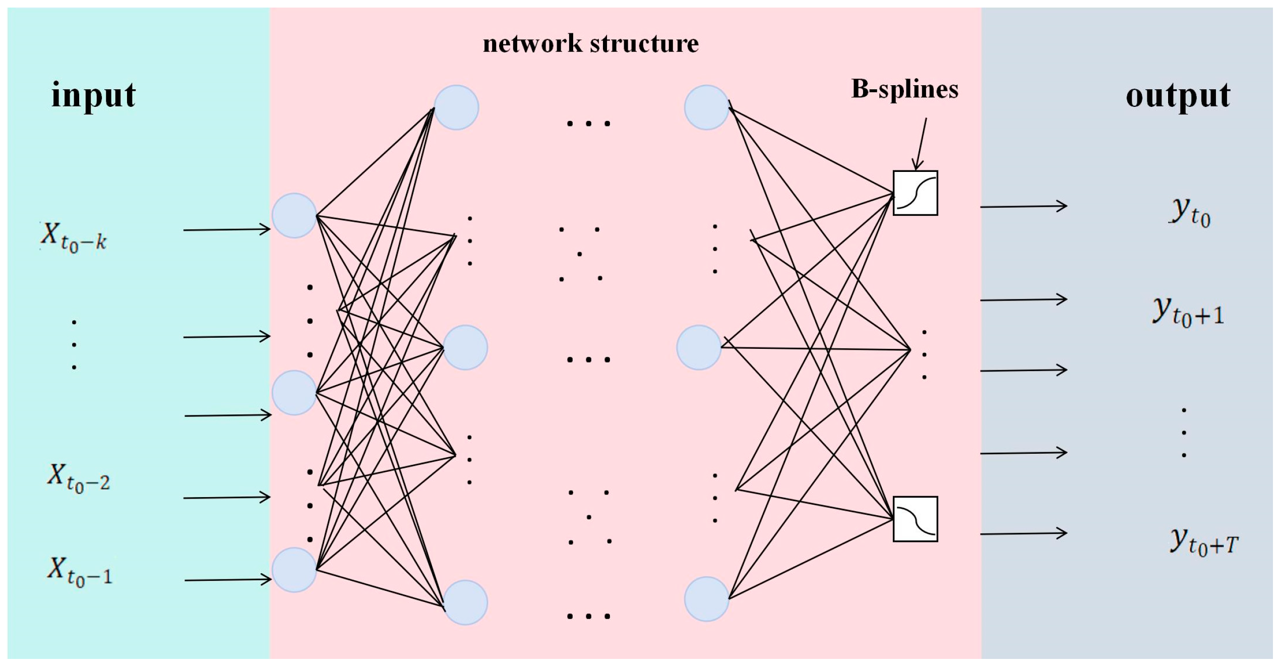
The electricity demand forecasting problem is formulated as a supervised learning task, where input–output pairs $\left\{X_{t_0-k:t_0-1},Y_{t_0:T}\right\}$ represent the context and prediction lengths. The goal is to find a function g that approximates $Y_{t_0:T}$. In this framework, three different time series models are employed: Transformer, TCN, and BiLSTM. Despite differences in their architectures, the models share a common structure. The output and input layers will comprise the $N_{out}$ and $N_{in}$ nodes, while the hidden layer comprise n nodes. Each model then processes the input sequence through its core structure. Following these processing steps, the output is passed to a KAN layer. The framework can be expressed by the:

$$y=f_{\mathrm{time}}\circ \mathsf{\Phi }$$

(18)

where $\mathsf{\Phi }$ is defined the KAN layer, $f_{time}$ denotes the time series models. The schematic diagram of the network structure is depicted in Figure 4.

3.6. The Experimental Framework

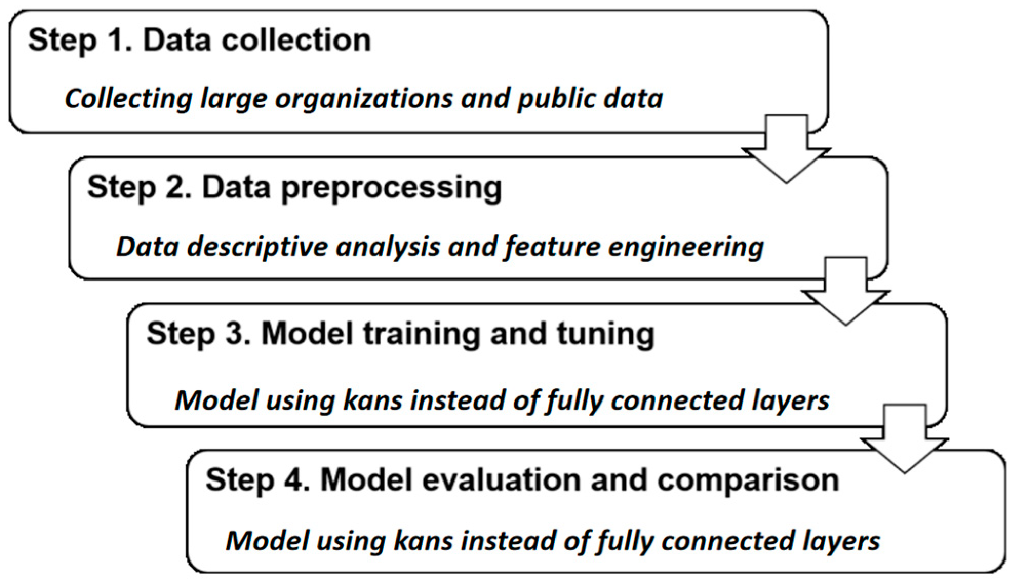
The research process is divided into four consecutive steps (Figure 5). In step 1, data is collected from large organizations and public sources. In step 2, the data is initially processed, including handling missing values, outliers, data scaling, etc. In step 3, the prediction model is trained and optimized. In step 4, cross-validation is performed to evaluate the performance of the prediction model.

Step 1: Drawing from multiple information sources, this study comprehensively analyzes the key factors influencing regional electricity demand to establish a robust feature selection framework. First, common feature variables were identified based on insights from classic literature in the field of electricity demand forecasting and related research. These variables include economic indicators, weather conditions, and historical power load data, all of which are widely recognized as having a significant impact on electricity demand. Additionally, the expertise of senior professionals from the power industry—spanning power generation companies, power dispatching departments, and power grid operation units—was leveraged. These experts, with extensive experience in the industry, provided valuable insights into the primary drivers of electricity demand through long-term practice. Using this background information, a preliminary candidate feature set was constructed. Next, the correlation between each feature and the target variable was evaluated using statistical and analytical techniques, such as mutual information and heatmap analysis, to eliminate low correlation or redundant features. Ultimately, an optimal feature set was determined for model construction and subsequent analysis.

Electricity-related data such as national demand, monthly electricity consumption of users, and regional power generation are downloaded and collated from the public website of the UK National Grid ESO. Financial and economic historical data are obtained from the large database of the data service provider Wind. Considering the impact of weather conditions on electricity demand, regional meteorological data are collected from the public website of the UK meteorological station, covering nine indicators from 2015 to 2024. Information such as the heat map and mutual information of factors is described in the second part.

Step 2: The model was developed and executed using Python in the PyCharm (Version Number 2024.3.2) environment. Preliminary descriptive statistical analysis of the dataset was conducted to address issues such as missing values and outliers. Basic visualization techniques were applied to gain a clear understanding of the data distribution, while the relationships between variables were examined using heatmaps and mutual information analysis. Outliers were identified during the preliminary analysis using the interquartile range method and were replaced through median interpolation. The missing rates for the dataset are detailed in

Table 2. Factors missing value ratio.

Factors	Missing Value Ratio
National demand—nd	1.5%
Electricity consumption—x2	1.3%
England electricity generation—x3	2.1%
Wales electricity generation—x4	2.6%
Regional Total precipitation—x5	4.3%
Regional average temperature—x6	2.1%
Regional average wind speed—x7	5.6%
Regional economy—x8	7.1%
Transmission system demand—x9	2.4%

. To handle missing values efficiently, feature engineering techniques were employed alongside the trend extrapolation method. The trend extrapolation method was specifically chosen for its ability to preserve inherent trends and temporal dependencies within the dataset.

The data was standardized using z-score standardization (Equation (19)). Where $x_{ij}$ represents the j-$\mathrm{t}\mathrm{h}$ observation of the i-$\mathrm{t}\mathrm{h}$ variable in the dataset, while $Mea{n}_i$ and $St{d}_i$ represent the mean and standard deviation of the i-$\mathrm{t}\mathrm{h}$ variable, respectively. The standardized data after processing is denoted as ${\overline{x}}_{ij}$.

$${\overline{x}}_{ij}={\displaystyle \frac{x_{ij}-Mea{n}_i}{St{d}_i}}$$

(19)

Step 3: A sliding window approach was applied to structure the input data for the model. During the experiments, different window sizes, including 10, 15, 20, and 30, were evaluated to determine the best value for capturing temporal dependencies in the time series data. A window size of 20 was chosen because it consistently achieved the best performance in both RMSE and MAE, the optimal window size is determined by grid search. This approach ensures that temporal dependencies within the time series data are preserved, allowing the model to learn sequential patterns effectively. All input and target features are scaled to the range of [−1, 1] to ensure data processing on a unified scale, thereby enhancing training efficiency and prediction accuracy.

Training and tuning the regional electricity demand forecasting models were conducted using three time series forecasting models, namely, the Transformer model, BiLSTM model, and TCN model, integrated with Kolmogorov–Arnold Networks (KANs). The forecasting indicators are compared with those of traditional models such as LSTM and GRU. Based on existing literature, these models were selected to capture the complex dependencies in the data. Use the preprocessed dataset in step 2 to train the model. To improve model predictive performance, the models were carefully tuned, and the best combination of parameters was identified using a grid search method. The dataset is divided into two parts, 80% for training and the remaining 20% for testing. Early stopping was also employed to prevent overfitting and further enhance model generalizability. In the KAN structure, the activation function employed was SiLU, with a grid size of 200. The weights between the adaptive and uniform grids were set to 0.02, and the noise scale of the spline weights was set to 0.1.

Step 4: To assess the predictive performance and accuracy of the models, we used the following indicators: mean squared error (RMSE), mean absolute error (MAE), the coefficient of determination (R²), and Akaike Information Criterion (AIC).

4. Experimental Results and Discussion

The results demonstrate that these methods and strategies significantly improve the model’s forecasting accuracy and generalization capacity, providing robust support for future electricity demand forecasting. Throughout the training process, the MAE, RMSE, R², and AIC values for each epoch were recorded, and the models with traditional LSTM and GRU indicators were compared. Radar diagrams of various metrics are shown in Figure 6. These metrics are used to assess the model’s goodness of fit and forecasting performance on the training set. For demonstration purposes, data from 2024 to the present were sampled. 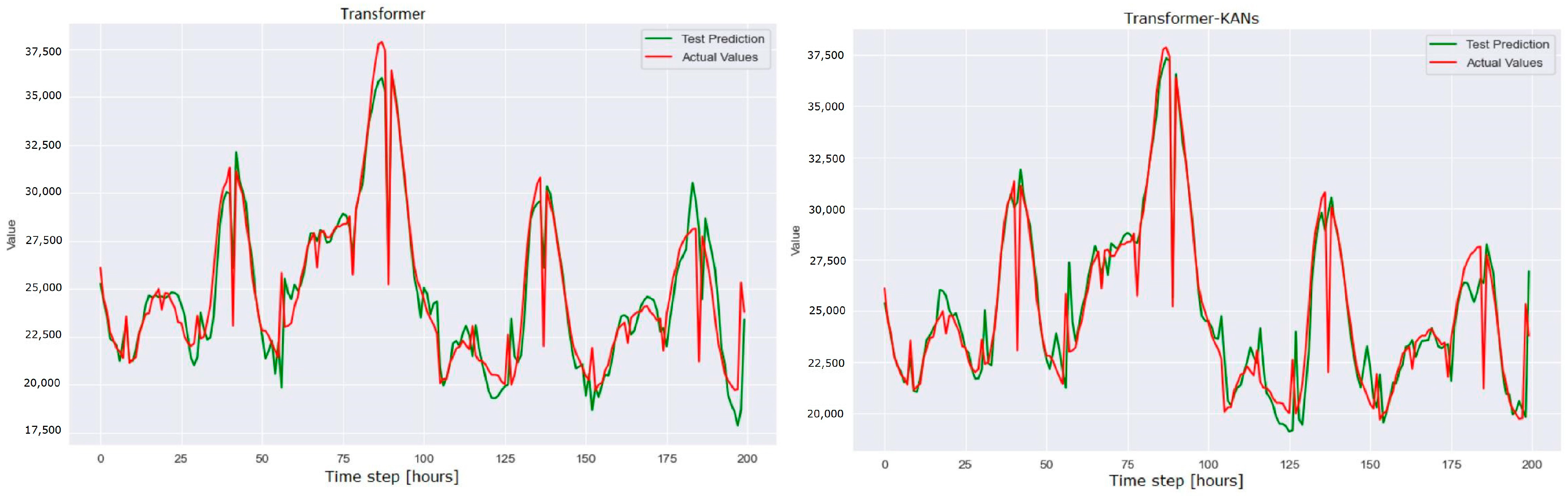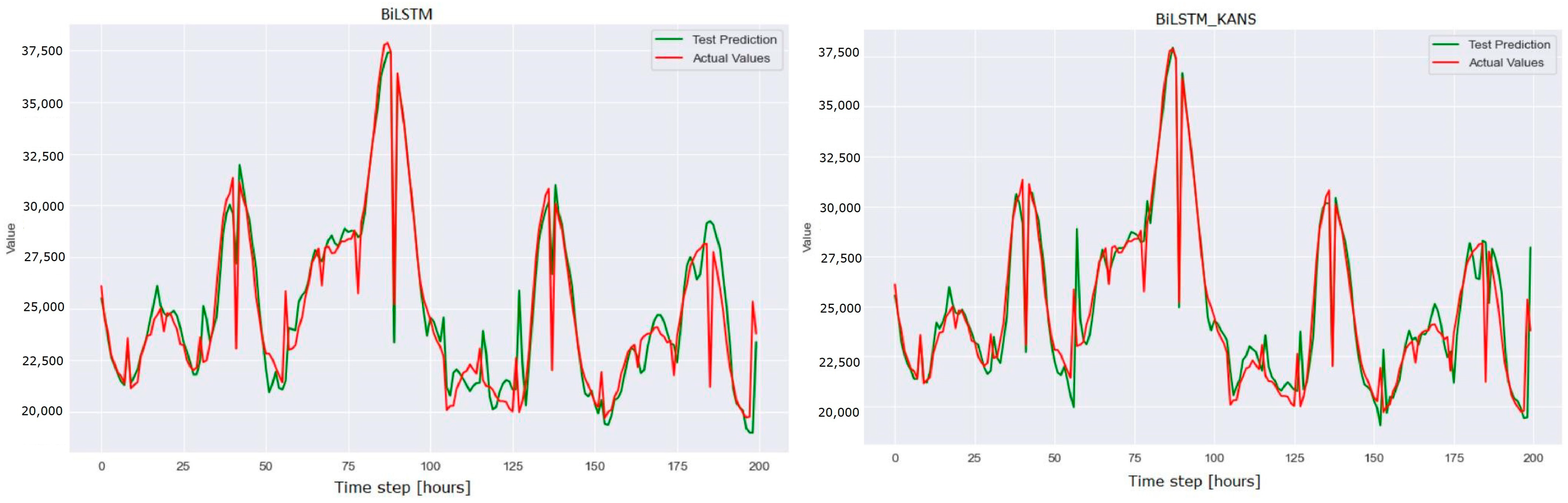Figure 7, Figure 8 and Figure 9 depict the actual input values (red) and test forecasted values (green). Comparing the actual values with the forecasted values reveals that the KAN-based model generates smoother forecasts and exhibits smaller errors across various time periods, particularly when addressing erratic fluctuations in the data. This advantage is particularly crucial in long-term time series forecasting tasks, as it delivers more reliable forecasts, offering valuable insights for practical applications.

As shown in

Table 3. Various metrics in the Test Set.

Model	RMSE	MAE	${\mathbf{R}}^2$	$\mathbf{AIC}$
LSTM	0.093	0.071	0.8945	−2103.21
GRU	0.098	0.083	0.9092	−2050.70
TCN	0.086	0.061	0.9362	−2235.67
TCN_KAN	0.075	0.053	0.9672	−2360.72
Transformer	0.095	0.068	0.9136	−2187.03
Transformer_KAN	0.083	0.059	0.9435	−2286.13
BiLSTM	0.085	0.061	0.9262	−2246.35
BiLSTM_KAN	0.083	0.059	0.9513	−2286.13

that TCN-KANs, Transformer-KANs, and BiLSTM-KANs exhibit improved RMSE and $\mathrm{ }{\mathrm{R}}^2$ compared to their original models (TCN, Transformer, and BiLSTM). Specifically, when comparing TCN-KANs with TCN, the introduction of the KANs network reduces the TCN model’s RMSE and MAE by 0.011 and 0.006, respectively, and ${\mathrm{R}}^2$ enhanced by 0.031. This signifies improved accuracy in electricity demand forecasting and effective prediction error reduction, indicating that the addition of the KANs network enhances the TCN model’s feature extraction and data pattern capturing capabilities. The AIC indicator is employed for model selection, as it balances model fit and complexity while evaluating the relative quality of statistical models by penalizing overfitting. A lower AIC value indicates better model prediction performance [47]. Both TCN-KANs and TCN achieve a smaller AIC value of 125.05, demonstrating their superior ability to balance accuracy and complexity. Compared to the indexes of traditional LSTM and GRU models, the proposed approach demonstrates significant improvements in performance metrics.

Similarly, comparing Transformer-KANs with Transformer, the introduction of the KANs network reduces the Transformer model’s RMSE and MAE by 0.012 and 0.009, respectively, and ${\mathrm{R}}^2$ enhanced by 0.0299. Both Transformer-KANs and Transformer achieve a smaller AIC value of 99.1, and the indicators are better than those of radical LSTM and GRU models. This demonstrates improved accuracy through better capture of complex patterns and global dependencies, highlighting the KANs network’s role in enhancing feature representation and reducing overfitting.

When comparing BiLSTM-KANs with BiLSTM, the introduction of the KANs network reduces the BiLSTM model’s RMSE and MAE by 0.002, ${\mathrm{R}}^2$ enhanced improvement by 0.0251. Both Transformer-KANs and Transformer achieve a smaller AIC value of 39.78. All indicators are better than LSTM and GRU. This improvement demonstrates the KANs network’s effectiveness in enhancing the BiLSTM model’s ability to capture and interpret time series data, thereby increasing prediction accuracy. Furthermore, this enhancement confirms the advantages of the KANs network in feature extraction and pattern recognition within the BiLSTM model.

To verify the performance of the proposed model, the widely recognized ETTh1 and ETTm1 datasets were used for evaluation, as shown in

Table 4. Various metrics in the ETTh1 and ETTm1.

Dataset	Model	RMSE	MAE	${\mathbf{R}}^2$
ETTh1	TCN	0.694	0.578	0.9162
	TCN_KAN	0.563	0.453	0.9672
	Transformer	0.682	0.568	0.9136
	Transformer_KAN	0.541	0.459	0.9435
	BiLSTM	0.793	0.661	0.9262
	BiLSTM_KAN	0.551	0.459	0.9513
ETTm1	TCN	0.629	0.524	0.9253
	TCN_KAN	0.476	0.402	0.9516
	Transformer	0.545	0.429	0.9373
	Transformer_KAN	0.442	0.386	0.9637
	BiLSTM	0.521	0.427	0.9165
	BiLSTM_KAN	0.458	0.392	0.9542

. The results indicate that the proposed model performs exceptionally well with respect to RMSE and MAE metrics. These findings validate the model’s effectiveness and generalizability for achieving accurate and dependable forecasting in practical scenarios.

In summary, it can be concluded that the introduction of the KANs network in the TCN, Transformer, and BiLSTM models has resulted in varying degrees of index reduction across all models, significantly improving forecasting performance. This demonstrates that the KANs network can further optimize feature extraction and pattern recognition capabilities within existing time series forecasting models, thereby enhancing overall forecasting performance. The findings of this study hold great significance for further refining time series forecasting models and improving the accuracy of electricity demand forecasting.

5. Conclusions

This work tackles the electricity demand forecasting problem by considering both common influencing factors and region-specific predictor variables. The proposed method integrates Kolmogorov–Arnold Networks (KANs) with prediction networks, demonstrating the potential and robustness of KANs in forecasting applications. Compared to traditional methods, the modified architecture significantly improves multi-step forecasting performance and stability, effectively addressing the long-term dependency issues often encountered in time series forecasting.

When compared to models such as LSTM, BRU, BiLSTM, TCN, and Transformer, the proposed architecture excels in long-term forecasting, showcasing its capacity to manage extended time horizons. By incorporating factors such as climate and economic variables, the model confirms the superior stability and effectiveness of KANs in processing real-world historical market data. These findings further validate the relevance and practicality of the Kolmogorov–Arnold Network framework for time series applications. The combination of the KAN network with other neural networks is driven by the complementary capabilities of these networks. While KAN excels at nonlinear feature extraction, it lacks the inherent ability to model temporal dependencies or global relationships, which are crucial for tasks such as time-series forecasting. Neural networks like BiLSTM, TCN, and Transformer specialize in capturing temporal and global patterns but often face challenges in capturing intricate nonlinear representations. Integrating KAN enhances these architectures by refining feature representation, thus improving predictive accuracy and robustness.

While the results of this study demonstrate the effectiveness of the proposed models, several limitations should be acknowledged. The findings are based on specific datasets and application scenarios. While the proposed models demonstrated strong generalizability in this context, and have been evaluated on the widely used ETTm1 and ETTh1 benchmark datasets, their applicability to other domains and data types requires further validation.

This study can be extended by incorporating additional machine learning techniques to further enhance the predictive framework. Balancing prediction accuracy, computational complexity, and practical applicability remains a critical aspect of future research. Considering data availability, it is important to focus on accumulating sufficient relevant industrial data to improve the robustness and real-world applicability of the proposed models. Additionally, future research should aim to quantify the impact of low-carbon transitions and economic development on regional electricity demand. This will help address emerging challenges in sustainable energy planning and provide more actionable insights for decision-makers.