Article

Particle Image Velocimetry Flow Characterisation of High-Convection Slot Nozzle Systems for Impingement Heat Transfer

Department for Industrial Furnaces and Heat Engineering, RWTH Aachen University, 52074 Aachen, Germany
*
Authors to whom correspondence should be addressed.
Energies 2025, 18(6), 1363; https://doi.org/10.3390/en18061363
Submission received: 15 February 2025 / Revised: 5 March 2025 / Accepted: 7 March 2025 / Published: 10 March 2025
(This article belongs to the Special Issue Heat Transfer Analysis: Recent Challenges and Applications)

Abstract

:
Impingement jets are used in many applications for high convective heat transfer. In order to optimise specialised nozzle systems, a comprehensive understanding of the gas flow is essential. The aim of this work is to investigate high-convective flows at Re = 10,000 to Re = 50,000 for a single slot nozzle (slot width W = 5 mm) and a slot nozzle array (distance between nozzle slots s = 70 mm) consisting of five nozzles. Particle image velocimetry measurements are taken for a distance between strip and nozzle exit of H = 50 mm and are compared to verify if the results from a single slot nozzle are transferable to a nozzle array. The presence of an array of nozzles not only creates a distinct zone where the individual jets interact but also changes the flow characteristics of the respective free jets. The potential core length in the nozzle field is significantly reduced compared to the single nozzle. It is therefore not possible to make a direct transfer of the results. Direct transferability of the results is therefore not possible. This means that further studies on whole arrays are needed to optimise nozzle arrays.

1. Introduction

Energy-intensive industries like metal, glass, or paper manufacturers use impingements jets to efficiently heat or cool products, where highly efficient nozzle systems are essential to minimise energy consumption [1]. Climate protection and resource efficiency are key issues in society and politics. Innovative and resource-efficient lightweight construction solutions are needed to reduce emissions and achieve our climate, sustainability, and electromobility goals [2]. High-strength aluminium and steel alloys are important factors for lightweight automotive construction. An amount of 100 kg less weight reduces the fuel consumption of a car by 0.7 l per 100 km. For electric vehicles a weight reduction is reflected in increased range. [3]. The materials optimised for these properties are characterised by demanding production routes, especially in terms of heat treatment. The complex requirements for the material properties place high demands on the nozzle systems. It is therefore imperative to continuously improve highly efficient nozzle systems for various applications across all industries.
Despite many studies [4] that have been carried out on impingement jets, further research is needed to optimise nozzle systems for specific applications with high Reynolds numbers Re > 10,000 due to the complex flow characteristics of impingement jets when striking a surface (see 
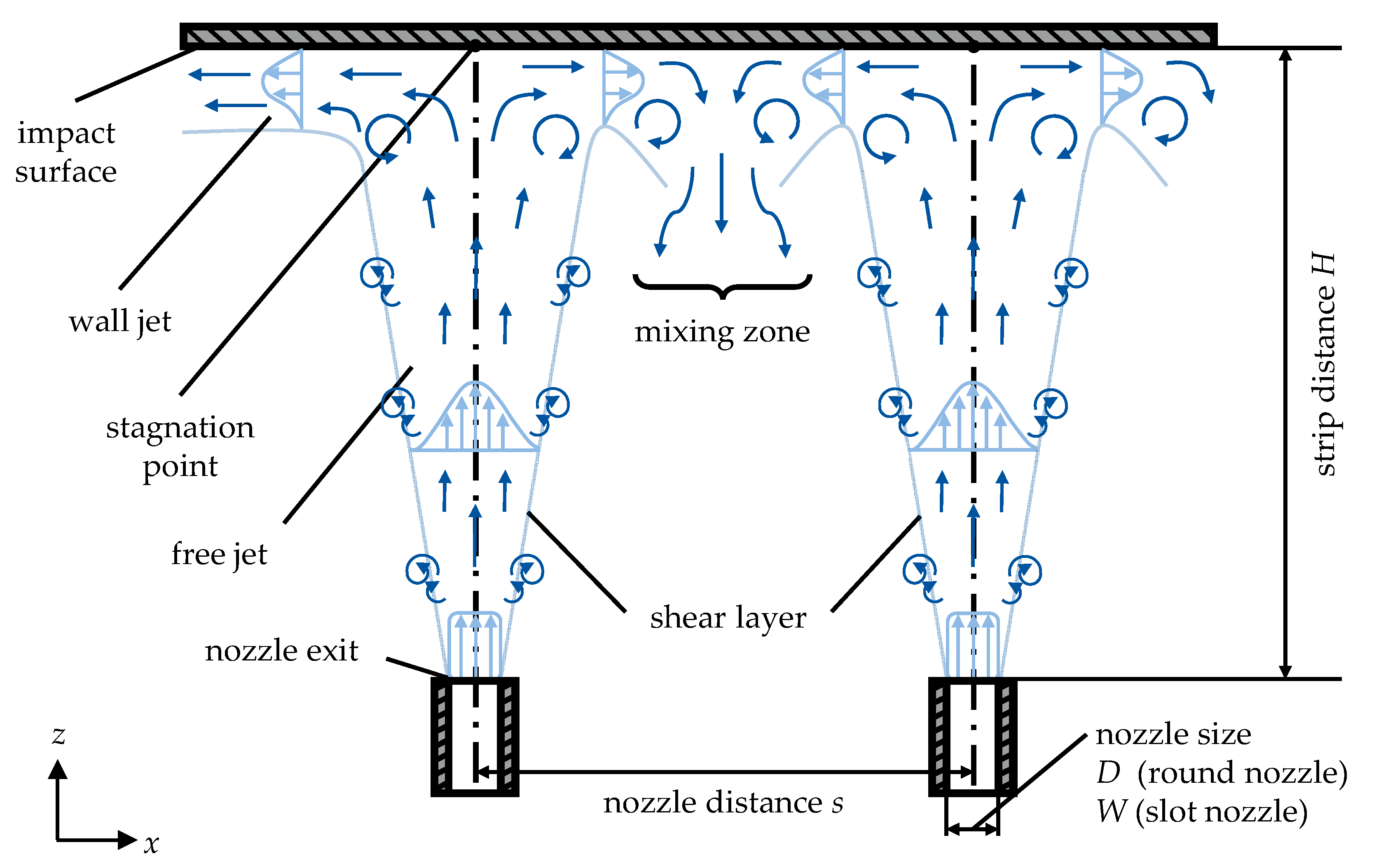
Figure 1). In this work, an industrial nozzle system used in the heat treatment of metal strips is analysed. The original nozzle array can be analysed without simplifications. An impingement jet can be divided into three zones: free jet zone, stagnation zone, and wall jet zone. For nozzle arrays an additional mixing zone is taken into consideration [5,6].
Starting from the nozzle, a free jet is formed which continuously expands and mixes with the surrounding medium (shear layer). As a result, the vertical velocity component decreases continuously until it is reduced to zero at the stagnation point. At the same time, the horizontal velocity component increases and a wall jet zone is formed. The area between individual nozzles in a nozzle field is referred to as a mixing zone. The characteristics of this flow depend on the nozzle geometry (round nozzle: nozzle diameter D, slot nozzle: slot width W), the distance between the nozzle outlet and the impact surface (strip distance H), the nozzle exit velocity u, and, in the case of a nozzle array, the distance between the individual nozzles s. In addition, the flow and therefore the heat transfer is very sensitive to the nozzle arrangement. A low ratio of strip distance to nozzle size is aimed for to maximise heat transfer but is not always technically feasible.
Within the free jet, the potential core jet is of importance for heat transfer. Here, the velocity remains constant and is equal to the nozzle exit velocity. The length of the core jet depends on the degree of turbulence of the nozzle flow and the nozzle exit velocity. The potential core jet length is defined as the position where the mean flow dynamic pressure (proportional to speed squared) reaches 95% of the initial value at the nozzle exit. For slot nozzles, the core jet length is between 4.7 and 7.7 times the nozzle width [7,8].
The basis for optimising nozzle systems is a sufficient understanding of the flow. The challenge is to visualise the real flows and their properties such as velocity and direction. One way to build up this understanding is through experiments supported by particle-based optical measurement techniques for describing velocities in flows. These include Laser Doppler Anemometry (LDA), Particle Image Velocimetry (PIV), Doppler Global Velocimetry (DGV), and Laser Transit Velocimetry (LTV) [9]. PIV’s ability to capture the flow velocity of a large number of points in an area simultaneously, the possibility for quantitative visualisation of flow structures, and gradient-based variables such as vorticity have led PIV to be used in various nozzle systems before [10]. Due to the wide range of applications of impingement jets, various optical flow investigations which have been carried out are summarised in Table 1.
Different types of nozzles and settings have been studied, including single nozzles and nozzle arrays with different shapes. The focus of the studies is also varied, e.g., Barbosa et al. [19,20] investigate the influence of the impact plate shape. Only a few studies deal with flows Re > 10,000, resulting in a specific field of research for highly convective heat transfer, which is characterised by very high flow velocities and special nozzle systems. In addition, often only individual nozzles are investigated, leaving the transferability of results to entire nozzle arrays limited. Especially for slot nozzle arrays, there is little data availability.
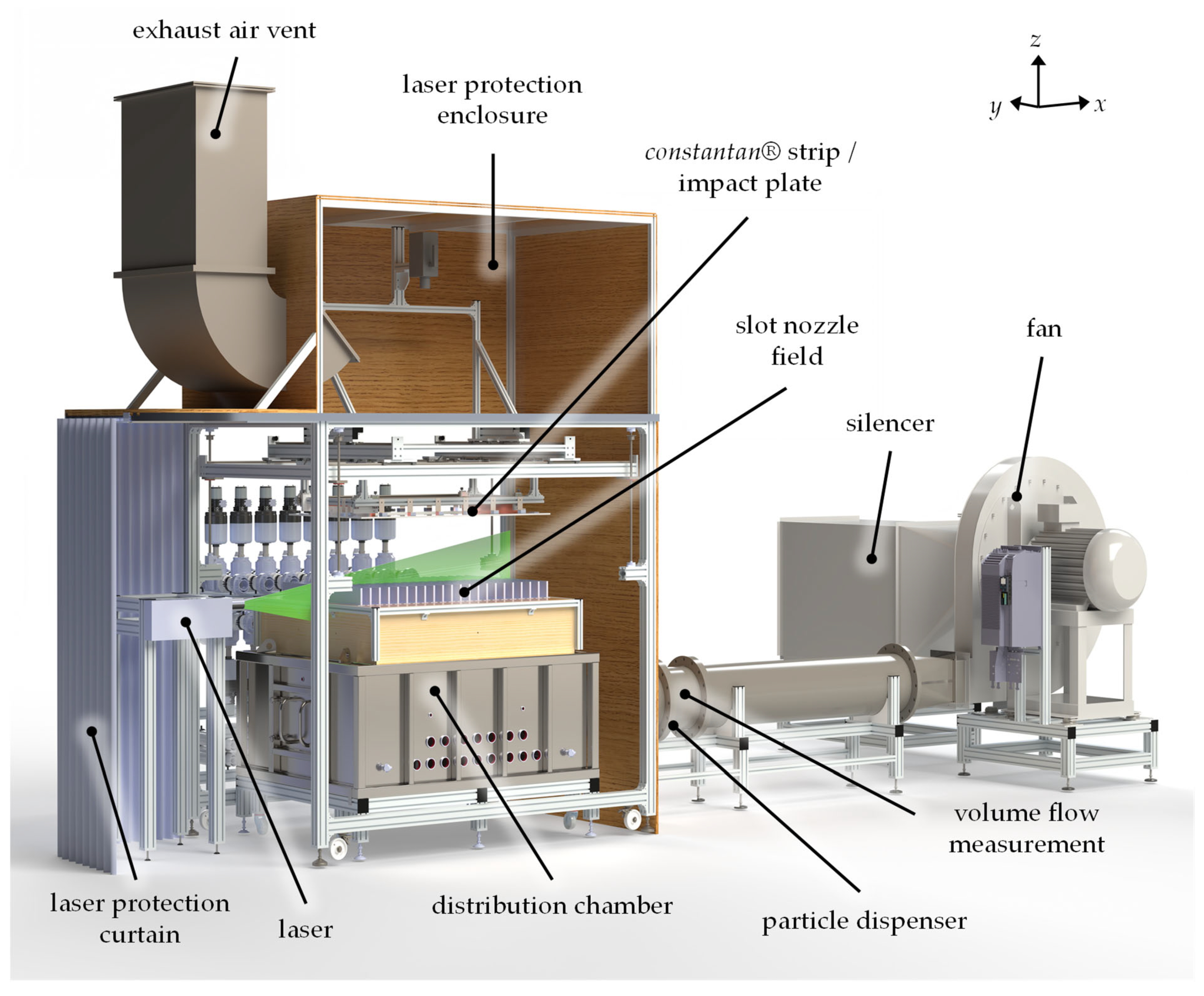
The aim of this study is to fill this research gap by investigating highly convective air flows at Re = 10,000 to Re = 50,000 using PIV. The experiments are carried out on a single slot nozzle and on an array of slot nozzles. In particular, the visualisation of the flow in entire slot nozzle arrays on an industrial scale in thermal process technology is unique.

2. Experimental Setup and Data Processing

2.1. Experimental Test Rig

The test rig for concluding the heat transfer of industrial nozzle systems by determining both the heat transfer coefficient and the flow visualisation is shown in Figure 2. The test rig is based on a radial fan with a power of 90 kWel and a maximum volume flow rate of 10,800 m3/h.
The fan draws in ambient air and accelerates it through an inlet section equipped with a flow meter into a distribution chamber. Particles are injected via the particle dispenser into the inlet section for visual observation of the flow. Various nozzle arrays up to industrial size (1480 × 1560 mm2) can be mounted on the distribution chamber. The heat transfer coefficient was calculated based on measurements taken from an IR camera directed at an electrically heated constantan® strip. For further technical details please refer to the detailed description which is included by Trampe and Rademacher in [21].
This test rig was extended by laser measurement technology including a Nd:YAG laser, a camera system, a particle dispenser, and laser protection to carry out optical investigations of the flows within various nozzle systems. In order to investigate the flow of the impinging jets using laser-optical measurement techniques, the heated strip is replaced by a steep plate. This provides an accurate and straight edge for alignment of the PIV camera system and protects the sensitive electrical connections from contamination by the tracer particles. In addition, the test rig was equipped with a full laser protection system.
The presented results are derived by an investigation of a single slot nozzle with a slot width of W = 5 mm and length of L = 100 mm. The slot nozzle array consists of five single slot nozzles (W = 5 mm, L = 100 mm). According to Holger [22] heat transfer reaches its maximum when Equation (1) is satisfied.
s o p = 7 5 H
Since the strip distance is kept constant at H = 50 mm, a nozzle spacing of s = 70 mm results. Accordingly, a flow-optimised slot nozzle array is assumed in this work. The geometric data of the investigated nozzle systems are summarised in Figure 3. The hydraulic diameter Dh is given for the dimensionless relations. For a slot nozzle, this is Dh = 2W.
The experiment utilised air as the test medium, with a temperature of TAir = 30 °C, resulting in a fluid density ρ = 1.161 kg/m3 and the dynamic viscosity η =17.1 µPa⋅s. The nozzle outlet velocity was determined through the usage of Equation (2) and the measurement of the dynamic pressure p at the nozzle outlet. Prior to each measurement, a pitot tube was installed and subsequently removed to avoid influencing the flow. The corresponding Reynolds numbers Re were calculated from the determined nozzle exit velocities using Equation (3).
u = 2 · p ρ
R e = ρ · u · 2 W η
For both nozzle systems three different nozzle exit velocities are investigated representing the range of different Reynolds numbers. Table 2 provides an overview of all tests carried out.
As part of the experimental investigation, a comparison of the outlet velocities of the single slot nozzle and the slot nozzle array was ensured, with a comparable value being recorded in each case. The nozzle outlet velocity that could be stably set for the single slot nozzle was labelled u = 19.3 m/s, which is 4 m/s higher than that of the slot nozzle array. It was not possible to set a lower volume flow with the fan. Opening the nozzle box could have caused cross-flow.

2.2. Measurement Setup

The measurement setup for carrying out PIV measurements includes a laser, a high-resolution camera, and a computer for recording and processing the data. A double-pulsed Nd:YAG laser (wavelength 532 nm) from Litro Lasers Ltd. is used. The maximum pulse energy is 200 mJ with a pulse length of 6–9 ns. The repetition rate can be adjusted between 0–15 Hz. The light sheet of the laser has a width of 2 mm. The liquid di-ethyl-hexyl sebacate (DEHS) is used as tracer particles for applications in air. This odourless and colourless liquid has a density of ρp = 0.912 g/cm3 and, using a seeding device from LaVision, has an average particle size of dp < 1 µm [23].
The high-resolution Imager digital camera CX2-16 from LaVision is integrated into the test rig. The camera is aligned at 90° to the laser sheet with a distance of approximately 880 mm. The maximum resolution of the camera is 5312 × 3024 pixels. The image dimensions are 241.5 × 137.5 mm, obtaining a resolution of 22 pixels/mm. LaVision’s DaVis 11 software is used for the processing of the measurement data. The local velocity vectors are calculated by cross-correlation, which is the basis for evaluating the PIV method [24]. For this purpose, the two recorded images are divided into frames of 64 × 64 pixels. An overlap factor of these frames is set on 75%. Further processing is used to reduce reflections and background noise. The background is deducted over a spatial length of 4 and a filter is used to remove or insert any outliers. In the following measurements, all outliers above 0.5 are removed and those below 3.0 are reinserted. Due to the processing parameters 20 vectors per orifice width are counted.

3. Results

The velocity and the turbulent kinetic energy (TKE) k distributions are determined for each case from the vector fields of the PIV measurements. While the velocity is derived directly from the vector displacement of the particle motion, the turbulent kinetic energy is calculated based on the Reynolds stress Rxx and Ryy according to Equation (4).
k = 3 4 R x x + R y y
Since a 2D planar PIV system is used in the present study, the turbulent kinetic energy can only be calculated in the laser slice plane with the vector components Vx and Vy. It is assumed that the turbulent kinetic energy in the third not-measured dimension Vz has the same dimension as Vx and Vy [25]. Turbulent kinetic energy characterises the energy in the fluctuating velocity field and can therefore be understood as a measure of the energy content of the turbulent motion in a flow. Since it is well known that heat transfer increases with increasing turbulence, knowledge of the distribution of turbulent kinetic energy is an important contribution for the optimisation of nozzle systems [26].
The singe-slot nozzle was measured within a range from x = ± 40 mm. The measurement of the slot nozzle array focused on the middle three nozzles (x = ± 90 mm). This allows the influence of increasing nozzle exit velocities on the formation of flow structures to be analysed. In addition, for the slot nozzle array, the interaction between the nozzles can be evaluated. To ensure a visual comparison of the data between the results of the single slot nozzle and the slot nozzle array, the scales per nozzle exit velocity have been kept the same. However, it should be noted that the TKE values of the slot nozzle array exceed the maximum value of the scale. Adjusting the scales to present the results of the single slot nozzle would result in a significant loss of information. This also applies to standardised scaling over the velocities.

3.1. Single Slot Nozzle

Initially, the flow through a single slot nozzle with a strip distance of H = 50 mm is analysed at different nozzle exit velocities. 
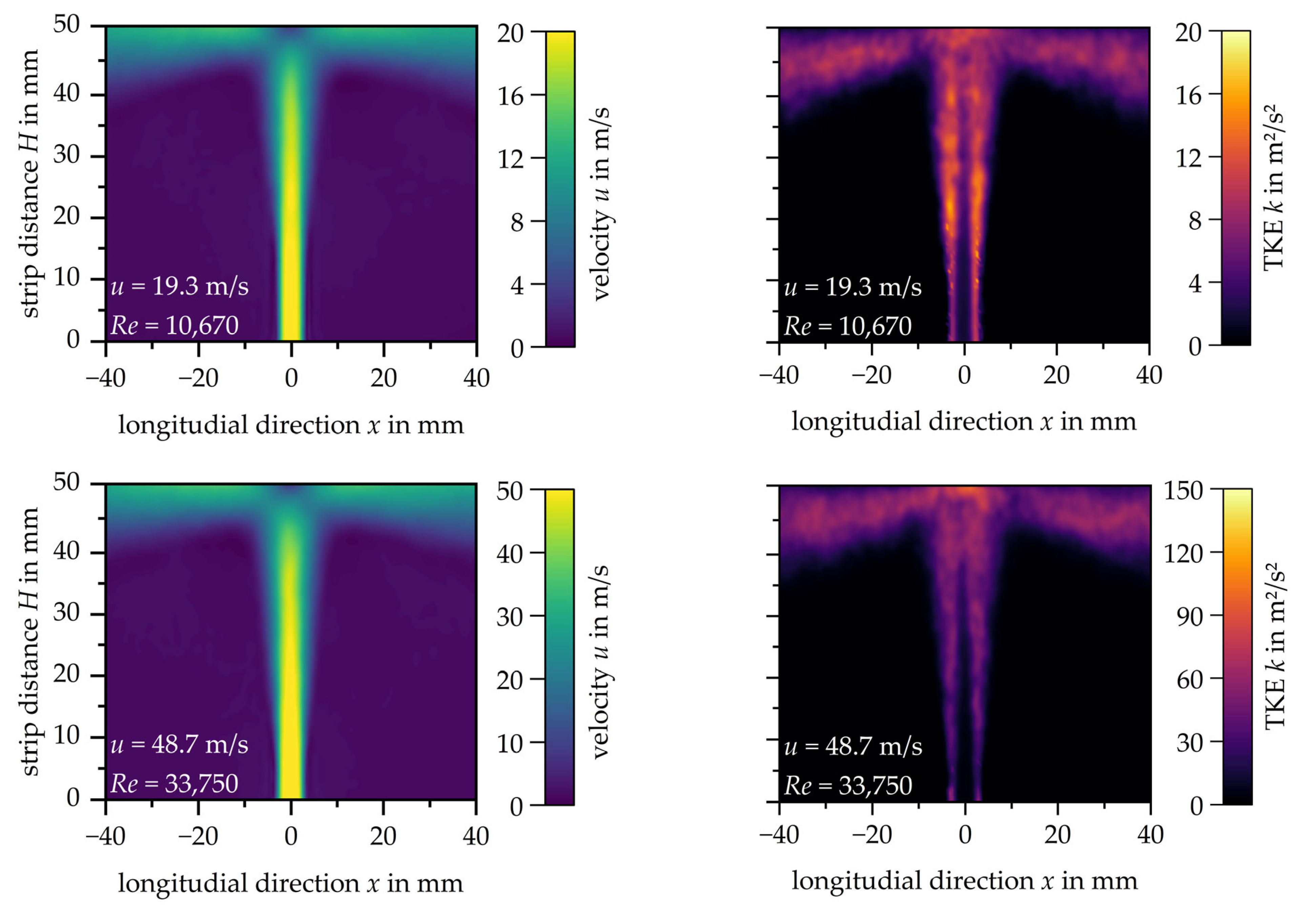
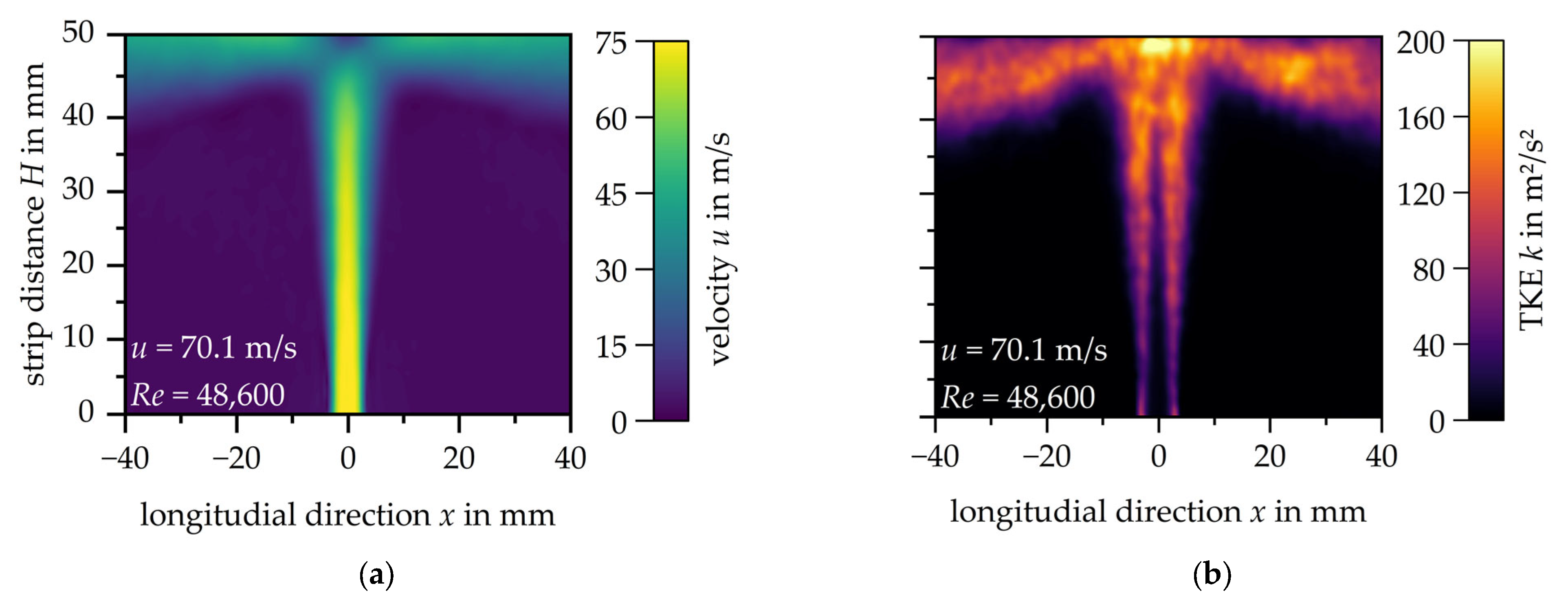
Figure 4a shows the velocity distributions for the three different exit velocities, while Figure 4b illustrates the corresponding distributions of turbulent kinetic energy. Note that the scales had to be adapted to the increasing exit velocity. A uniform scaling across all velocities leads to reduced contrast, resulting in reduced readability of the measured data.
The influence of the nozzle exit velocity u on the flow is limited since only higher velocities in both the free jet and the wall jet can be observed. The dimension of the stagnation zone remains unaffected, as does the expansion of the shear layer.
The distribution of turbulent kinetic energy (TKE) throughout the impingement jet changes with increasing nozzle exit velocity. Turbulent kinetic energy is generally lowest in the centre of the free jet and wall region and highest in the shear layers of the free jet and the wall jet. The formation of the impingement jet is symmetrical.
For the lowest nozzle exit velocity of u = 19.3 m/s (Re = 10,670), the highest turbulent kinetic energy of k = 15 m2/s2 is reached in the shear layer of the free jet. The turbulent kinetic energy increases with increasing nozzle exit velocity at u = 48.7 m/s and reaches its maximum at the stagnation point at k = 95 m2/s2. The wall jet reaches a turbulent kinetic energy value up to k = 65 m2/s2. In the shear layer of the free jet a turbulent kinetic energy of k = 40 m2/s2 is reached.
At the maximum investigated nozzle exit velocity u = 70.1 m/s, the turbulent kinetic energy reaches up to k = 200 m2/s2 at the stagnation point. It is noticeable that the zone of increased turbulent kinetic energy in the area of the stagnation point expands as the nozzle exit velocity increases. Analogous to the doubling of the turbulent kinetic energy at the stagnation point of the impingement jet by increasing the nozzle exit velocity from u = 48.7 m/s to u = 70.1 m/s, the turbulent kinetic energy in the wall jet (k = 134 m2/s2) and in the shear zone (k = 89 m2/s2) also doubles.

3.2. Slot Nozzle Array

Single nozzles are not commonly used in an industrial setting; therefore, a slot nozzle array consisting of five single slot nozzles is considered. The flow from the three centre nozzles is evaluated as it is anticipated that the flow formation will repeat symmetrically. The left nozzle appears to be slightly displaced inwards. This, however, does not affect the key findings of the study. Figure 5a shows the velocity distribution of the slot nozzle array at a nozzle exit velocity of u = 15.4 m/s.
The impingement jets from each of the three nozzles are clearly visible. The mixing zone between the left and middle nozzle is more pronounced than the mixing zone between the middle and right nozzles. This is also apparent in the distribution of turbulent kinetic energy in Figure 5b. There are local maxima of k = 20 m2/s2 both in the shear layer of the individual free jets and in the area of the mixing zone where two wall jets meet. The distribution of the turbulent kinetic energy in the individual impingement jet is not symmetrical.
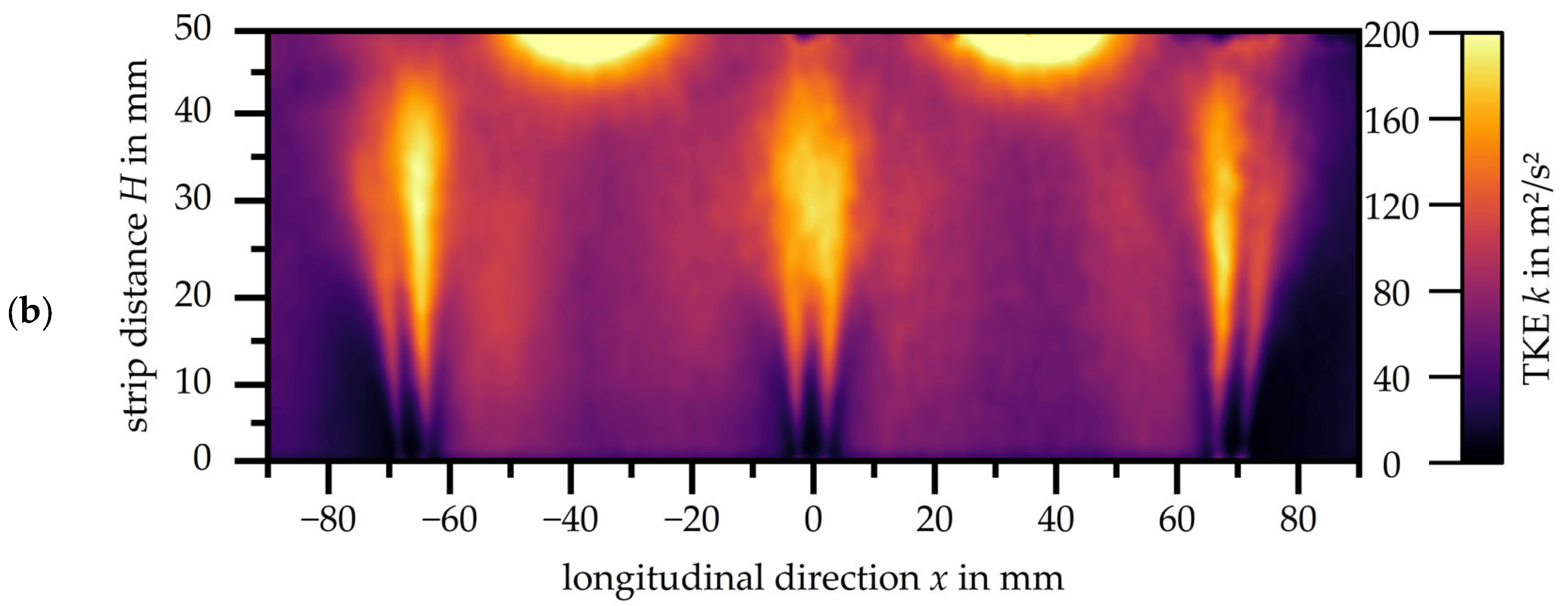
Figure 6 provides in (a) the velocity distribution and in (b) the turbulent kinetic energy distribution of the slot nozzle array with a nozzle exit velocity of u = 48.7 m/s. Due to the increased nozzle exit velocity, the velocity in the wall jets also increases, resulting in a clearer formation of the wall jet flow and the flow in the mixing zone.
The areas with high turbulent kinetic energy have increased significantly in proportion. After just one third of the free jet, a turbulent kinetic energy of k = 170 m2/s2 is reached in the entire impingement jet. The zone around the interaction between two wall jets has also increased and reaches a turbulent kinetic energy of k = 200 m2/s2. It is now noticeable that the mixing zone extends between the nozzles. There is no change in the flow characteristics when the nozzle exit velocity is increased up to u = 70.1 m/s in the slot nozzle array (see Figure 7).

3.3. Uncertainty

The most important criterion for PIV measurements is that the tracer particles follow the flow for any velocity u without delay. The Stokes number, as shown in Equation (5), is used to verify this criterion. For Stk << 1 the particles follow the flow closely [9].
S t k = τ p τ f
Therefore, τ p describes the response time as defined in Equation (6) and τ f is the characteristic time scale of the flow (see Equation (7)) [24].
τ p = d p 2 · ρ p 18 · μ
τ f = L u
The response time formula is valid for Re < 1. For the velocity range studied, Re is in the interval of Re = 10,000 to 50,000 (see Table 2). Due to the high Reynolds numbers, an additional factor, a standard drag correlation CD, must be added [27]. The material data of the DEHS tracer particles (particle diameter dp, particle density ρ p ) were mentioned in Section 2.2; the dynamic viscosity of the air is specified as μ = 1.185 · 10−5 Pa · s. With the characteristic length of the slot nozzle L = Dh = 2W and the additional factor CD, this results in τ p being between 1.86 · 10−6 s–1.98 · 10−6 s. This leads to Stokes numbers between Stk = 0.00353–0.01384. Due to the small Stokes numbers for all velocities, the tracing error can be estimated to be less than 1% [9].
The overall measurement uncertainty is also analysed directly in the software DaVis based on the uncertainty of standard deviation [25]. According to Wieneke [
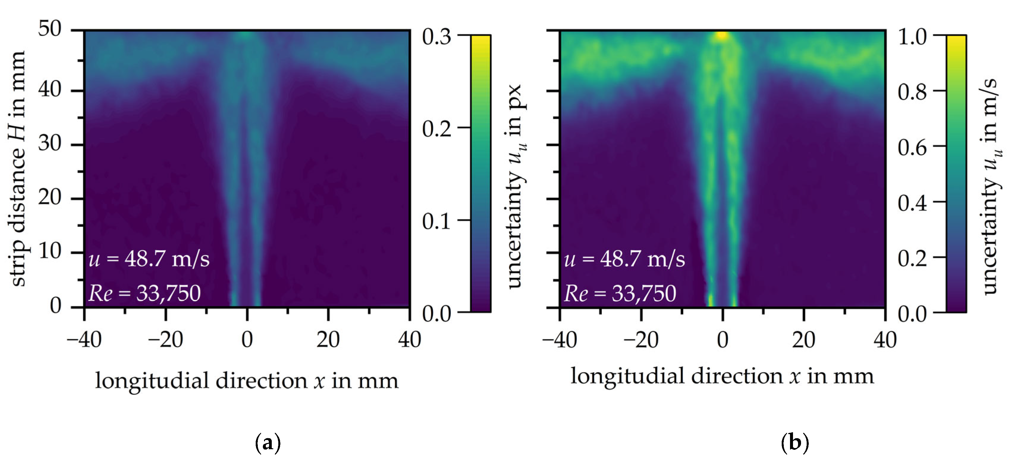
28], a value of 0.01 pixels is considered ‘excellent’ and 0.3 pixels ‘poor’. As an example, the measurement uncertainty is illustrated by the single slot nozzle with a nozzle exit velocity of u = 48.7 m/s in Figure 8. The measurement uncertainty of the velocity distribution uu is shown in pixels in Figure 8a and in m/s in Figure 8b. At this point, both units are selected in order to show the accuracies of the PIV measurement carried out in pixels but also the more comprehensible deviation of the velocity distribution in m/s.
The measurement uncertainty of the PIV measurements is on average less than uu < 0.1 px, except for the stagnation point, where the measurement uncertainty reaches its maximum deviation at uu = 0.16 px. The illustration in Figure 8b shows that the corresponding measurement uncertainty is uu = 0.5 m/s on average and the increased measurement uncertainty at the stagnation point is uu = 1 m/s.
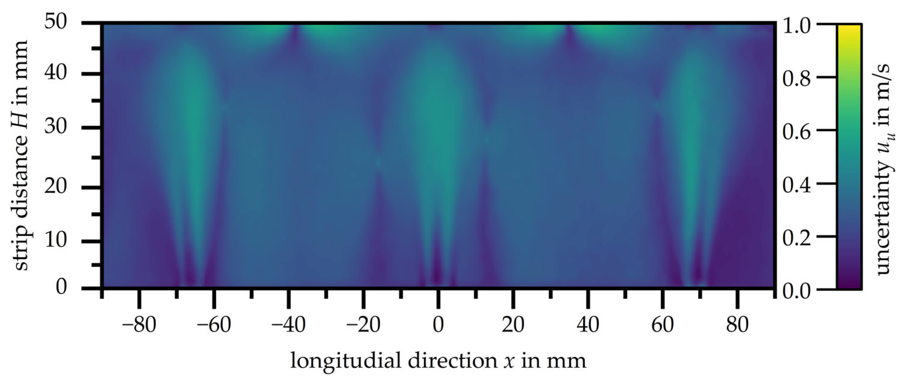
Figure 9 presents the measurement uncertainty uu of the velocity distribution of the slot nozzle array with a nozzle exit velocity of u = 48.7 m/s, given in m/s. As with the single nozzle, the accuracy of the PIV in pixels is less than 0.1 px.
The measurement uncertainty of the other investigated nozzle exit velocities are within the shown range and can be considered overall as ’good’ according to Wieneke [28]. Higher accuracies, especially in the area near the stagnation point, have to be accepted at this point, as the focus is on a comprehensive flow investigation of the impingement jets. A high-resolution analysis of the boundary layer is beyond the scope of this study.

4. Conclusions

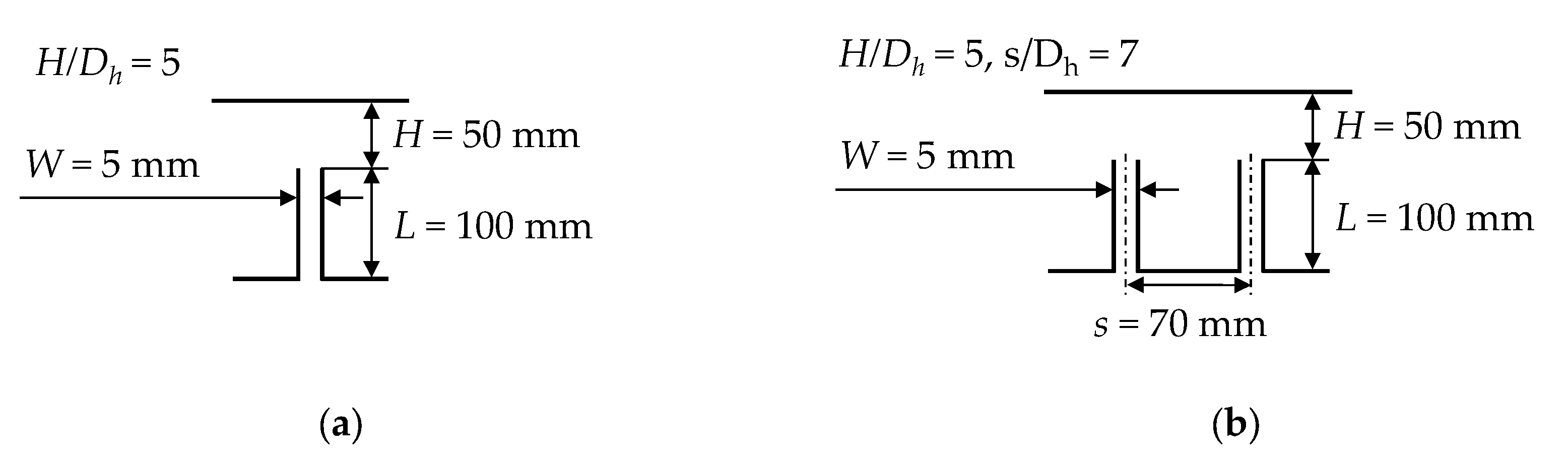
The highly convective flow of an impingement jet generated by a single slot nozzle (W = 5 mm) and a slot nozzle array consisting of five single slot nozzles with a nozzle spacing of s = 70 mm have been investigated for three different nozzle exit velocities. The nozzle exit velocities correspond to Reynolds numbers from approximately Re = 10,000 to 50,000. The resulting flow profiles of the single slot nozzle and the slot nozzle array are subsequently compared and evaluated.
The results for the single slot nozzle show that the formation of the characteristic flow pattern is independent from the nozzle exit velocity leading to an increase in the mean velocity of the impingement jet. The same applies to the turbulent kinetic energy distribution. The turbulent kinetic energy increases reciprocal to the increase in velocity. The same was observed when analysing the slot nozzle array. Furthermore, it can be seen that the velocity in the mixing zone increases with increasing nozzle exit velocity, which leads to a higher turbulent kinetic energy. 
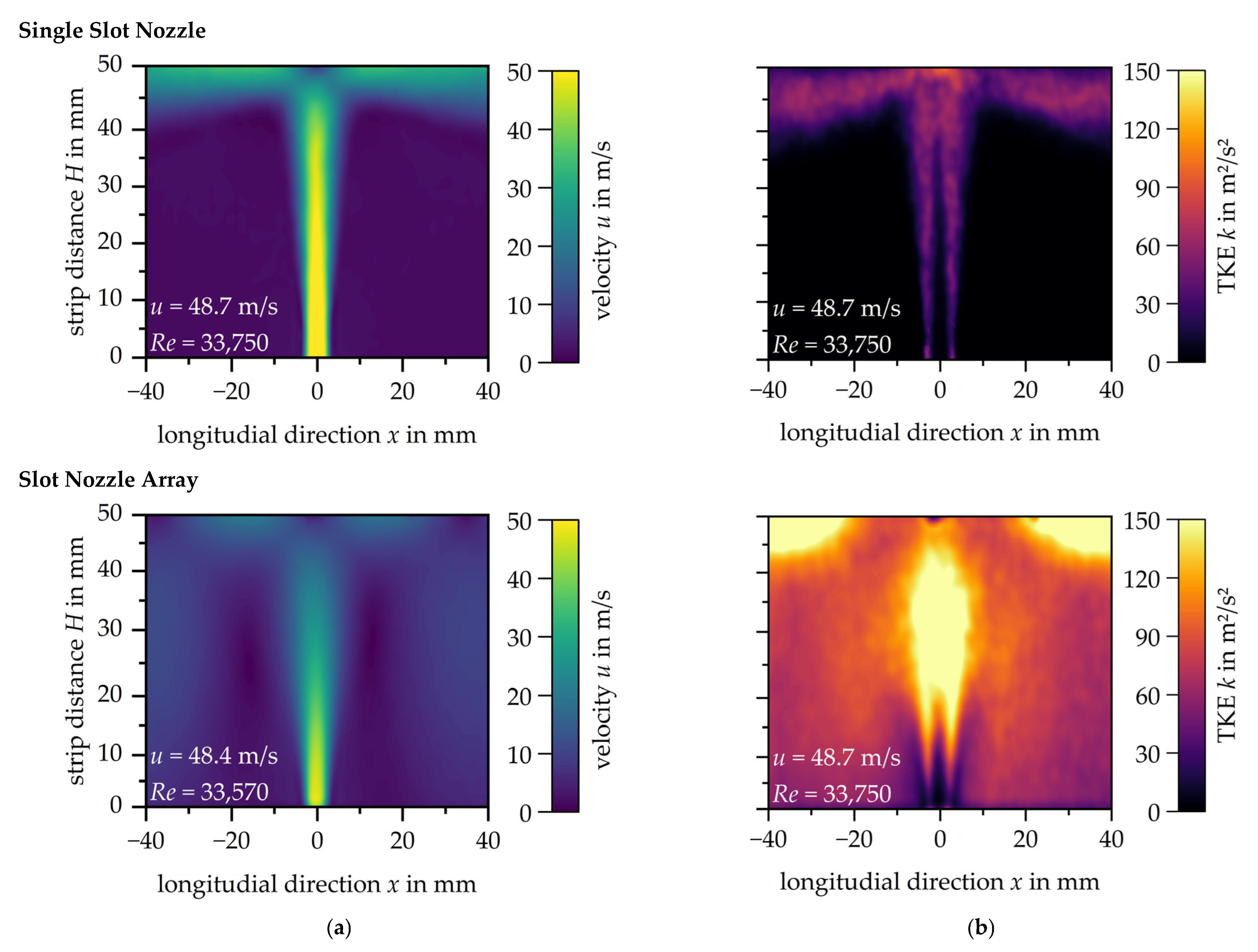
Figure 10 compares the results of the single slot nozzle and the slot nozzle array at a nozzle exit velocity of u ≈ 48.5 m/s. The central slot nozzle of the slot nozzle array has been selected for this comparison.
Comparison of the velocity profiles at the same nozzle exit velocity shows that the potential core jet length in the free jet of the impingement jet is about one third shorter for the centre nozzle of the slot nozzle array and therefore has a significantly lower velocity. Table 3 shows the theoretical velocities according to Livingood and Hrycak [7] for the associated nozzle exit velocities of the single slot nozzle as well as the centre nozzle in the slot nozzle array. The corresponding absolute core jet length and the core jet length as a function of the nozzle width W from the PIV measurement are also given in the table.
With a relative core jet length of between 6.4 and 6.9, the core jet length of the single slot nozzle is within the range predicted by Zuckermann [8]. The reduced relative core jet length of 1.3 to 2.8 in the centre nozzle of the slot nozzle array deviates significantly from this specification. In the area between the core jet and the impact surface, a substantial reduction in the velocity of the impingement jet can be recognised.
In the mixing region of the impingement jet a higher velocity is observed due to the interaction with the adjacent jets for the slot nozzle array. The turbulent kinetic energy in the shear layer and in the area of the wall jet where the jets meet is three times higher compared to the single slot nozzle. Even between the nozzles, away from the shear layer, the turbulent kinetic energy is significantly higher. The reverse is observed at the stagnation point. Due to the reduced velocity in the stagnation zone of the slot nozzle array, no local maximum of the turbulent kinetic energy is reached here.
This finding leads to the conclusion that interference between multiple impinging jets is not limited to the mixing zone near the wall. The mixing zone partially extends along the length of the jet, resulting in further interaction with the jet. This leads to a significant reduction in the velocity of each individual impingement jet, but also to a disproportionate increase in turbulent kinetic energy. Geers [13] made similar observations when analysing single round nozzles and a round nozzle array. The flow in round nozzles is rotationally symmetrical, which is not the case with slot nozzles. Therefore, the results cannot be directly compared to each other. Nevertheless, this work confirms that it is not possible to extrapolate the results of flow investigations on individual nozzles to entire nozzle fields, without compensating for the observed interaction. Further investigations with other nozzle arrangements are essential to confirm the observations of both studies. Larger nozzle spacings are expected to reduce the interaction between the impinging jets, but the effect on the core jet length is still largely unknown.
Due to the limited database for impingement flows from slot nozzle systems, there is a need for further research. Most of the work has been carried out on single nozzles, and the present work raises questions about the applicability of the flow results to nozzle arrays. For this reason, experimental and numerical investigations on impinging heat transfer problems, especially for industrial applications, must examine more nozzle arrays. Otherwise, the extrapolated results from single slot nozzles will not be sufficient for the efficient design of nozzle systems.

Author Contributions

E.T., I.D., D.B., H.P. and C.W. Conceptualization, methodology, software, validation, and formal analysis, investigation, resources, data curation, writing—original draft preparation, writing—review and editing, visualization, supervision, project administration, funding acquisition. All authors have read and agreed to the published version of the manuscript.

Funding

This research received no external funding.

Data Availability Statement

Data are contained within the article.

Acknowledgments

The presented experimental data were generated during trials within the IGF project (“Impingement jets—Development and experimental validation of numerical heat transfer models for impingement jets”; IGF no. 22751 N) funded by the Federal Ministry for Economic Affairs and Climate Action based on a resolution of the German Bundestag.

Conflicts of Interest

The authors declare no conflict of interest.

Nomenclature

The following abbreviations are used in this manuscript:
CDStandard drag correlation
DDiameter (round nozzle)mm
dpParticle diameterμm
HStrip distancemm
kTurbulent kinetic energym2/s2
LNozzle lengthmm
sopOptimised nozzle distancemm
ReReynolds number
Rxx, RyyReynolds stress
sNozzle distancemm
StkStokes number
uNozzle exit velocitym/s
uuUncertainty of the velocity distributionm/s, px
Vx, Vy, VzVector components
WWidth mm
XNumber of nozzles
μDynamic viscosityPa · s
ρpParticle densityg/cm3
ρFluidFluid densityg/cm3
τfResponse times
τpCharacteristic time scales

References

  1. Fleiter, T.; Rehfeldt, M.; Hirzel, S.; Neusel, L.; Aydemir, A.; Schwotzer, C.; Kaiser, F.; Gondorf, C.; Hauch, J.; Hof, J.; et al. CO2-Neutrale Prozesswärmeerzeugung; UBA: New York, NY, USA, 2023. [Google Scholar]
  2. European Parliament. Resolution of 15 January 2020 on the European Green Deal (2019/2956(RSP)). Available online: https://www.europarl.europa.eu/doceo/document/TA-9-2020-0005_EN.html (accessed on 4 March 2025).
  3. Umweltbundesamt. Ökosteuer—Sparen Oder Zahlen?: Sprit Sparen und Mobil Sein. 2009. Available online: https://www.umweltbundesamt.de/sites/default/files/medien/publikation/long/3705.pdf (accessed on 4 March 2025).
  4. Plant, R.D.; Friedman, J.; Saghir, M.Z. A review of jet impingement cooling. Int. J. Thermofluids 2023, 17, 100312. [Google Scholar] [CrossRef]
  5. Bergman, T.L.; Lavine, A.S.; Incropera, F.P.; Dewitt, D.P. Fundamentals of Heat and Mass Transfer; John Wiley & Sons: Hoboken, NJ, USA, 2011; ISBN 978-0470-50197-9. [Google Scholar]
  6. Hofmann, H.M. Wärmeübergang Beim Pulsierenden Prallstrahl; KIT Scientific Publishing: Karlsruhe, Germany, 2005; ISBN 3-937300-57-0. [Google Scholar]
  7. Livingood, J.N.B.; Hrycak, P. Impingement Heat Transfer from Turbulent Air Jets to Flat Plates: A Literature Survey. NASA-TM-X-2778. 1973. Available online: https://ntrs.nasa.gov/citations/19730016200 (accessed on 4 March 2025).
  8. Zuckerman, N.; Lior, N. Jet Impingement Heat Transfer: Physics, Correlations, and Numerical Modeling; Elsevier: Amsterdam, The Netherlands, 2006; pp. 565–631. ISBN 9780120200399. [Google Scholar]
  9. Springer Handbook of Experimental Fluid Mechanics; Tropea, C., Ed.; Springer: Berlin/Heidelberg, Germany, 2007; ISBN 9783540302995. [Google Scholar]
  10. Scharnowski, S.; Kähler, C.J. Particle image velocimetry—Classical operating rules from today’s perspective. Opt. Lasers Eng. 2020, 135, 106185. [Google Scholar] [CrossRef]
  11. Buchlin, J. Convective Heat Transfer in Impinging-Gas-Jet Arrangements. JAFM 2011, 4, 137–149. [Google Scholar] [CrossRef]
  12. Buchlin, J.-M.; Gouriet, J.-B.; Planquart, P.; van Beeck, J.; Renard, M. Experimental and Numerical Study of Convective Heat Transfer in an Array of Slot Jets. In Proceedings of the 2002 ASME Joint U.S.-European Fluids Engineering Conference, Montreal, QC, Canada, 14–18 July 2002; pp. 13–19, ISBN 0-7918-3616-9. [Google Scholar]
  13. Geers, L.F.G.; Tummers, M.J.; Hanjalic, K. Experimental investigation of impinging jet arrays. Exp. Fluids 2004, 36, 946–958. [Google Scholar] [CrossRef]
  14. Angioletti, M.; Nino, E.; Ruocco, G. CFD turbulent modelling of jet impingement and Its validation by particle image velocimetry and mass transfer measurements. Int. J. Therm. Sci. 2005, 44, 349–356. [Google Scholar] [CrossRef]
  15. Wang, H.; Lee, S.; Hassan, Y.A. Particle image velocimetry measurements of the flow in the converging region of two parallel jets. Nucl. Eng. Des. 2016, 306, 89–97. [Google Scholar] [CrossRef]
  16. Khayrullina, A.; van Hooff, T.; Blocken, B.; van Heijst, G.J.F. PIV measurements of isothermal plane turbulent impinging jets at moderate Reynolds numbers. Exp. Fluids 2017, 58, 31. [Google Scholar] [CrossRef]
  17. Nguyen, D.T.; Maher, B.; Hassan, Y. Effects of Nozzle Pressure Ratio and Nozzle-to-Plate Distance to Flowfield Characteristics of an Under-Expanded Jet Impinging on a Flat Surface. Aerospace 2019, 6, 4. [Google Scholar] [CrossRef]
  18. Berthold, A.; Haucke, F.; Weiss, J. Flow Field Analysis of a Dynamically Forced Impingement Jet Array. In Proceedings of the AIAA Scitech 2020 Forum, Orlando, FL, USA, 6–10 January 2020; American Institute of Aeronautics and Astronautics: Reston, VA, USA, 2020; p. 1062020, ISBN 978-1-62410-595-1. [Google Scholar]
  19. Barbosa, F.V.; Teixiera, S.F.; Teixeira, J.C. 2D PIV analysis of the flow dynamics of multiple jets impinging on a complex moving plate. Int. J. Heat Mass Transf. 2022, 188, 122600. [Google Scholar] [CrossRef]
  20. Barbosa, F.V.; Teixeira, S.F.C.F.; Teixeira, J.C.F. Flow dynamics and heat transfer characterization of confined multiple jets impinging on a complex surface. Exp. Fluids 2023, 64, 153. [Google Scholar] [CrossRef]
  21. Trampe, E.; Rademacher, N.; Wulfmeier, M.; Büschgens, D.; Pfeifer, H. A High-Resolution Method for the Experimental Determination of the Heat Transfer Coefficients of Industrial Nozzle Systems in Heat Treatment Plants. Appl. Sci. 2024, 14, 3024. [Google Scholar] [CrossRef]
  22. Martin, H. Heat and Mass Transfer between Impinging Gas Jets and Solid Surfaces. In Advances in Heat Transfer; Elsevier: Amsterdam, The Netherlands, 1977; Volume 13, pp. 1–60. ISBN 9780120200139. [Google Scholar]
  23. LaVision GmbH. Seeding Particles: DEHS. Available online: https://shop.lavision.de/en/seeding-particles/1/dehs (accessed on 4 March 2025).
  24. Raffel, M. Particle Image Velocimetry: A Practical Guide, 3rd ed.; Springer International Publishing AG: Cham, Switzerland, 2018; ISBN 9783319688527. [Google Scholar]
  25. LaVision GmbH. Product Manual for DaVis 11.0; LaVision GmbH: Göttingen, Germany, 2023. [Google Scholar]
  26. Pope, S.B. Turbulent Flows; 1. Publ., 12. Print; Cambridge University Press: Cambridge, UK, 2015; ISBN 9780521591256. [Google Scholar]
  27. COMSOL Multiphysics®. Users Guide 5.6: Theory for the Particle Tracing for Fluid Flow Interface; COMSOL: Stockholm, Sweden, 2020. [Google Scholar]
  28. Wieneke, B. PIV uncertainty quantification from correlation statistics. Meas. Sci. Technol. 2015, 26, 74002. [Google Scholar] [CrossRef]
Figure 1. Schematic illustration of the flow of an impingement jet.
Energies 18 01363 g001
Figure 2. Test rig for optical flow measurements and heat transfer characterisation; dimensions: 8 m × 5 m × 4 m.
Energies 18 01363 g002
Figure 3. Schematic of the investigated (a) single nozzle and the (b) slot nozzle array.
Energies 18 01363 g003
Figure 4. Representation of (a) the velocity and (b) the turbulent kinetic energy distribution for an impingement jet with three different nozzle exit velocities with H = 50 mm.
Energies 18 01363 g004aEnergies 18 01363 g004b
Figure 5. Representation of (a) the velocity and (b) the turbulent kinetic energy distribution for an impact jet array with a nozzle exit velocity of u = 15.4 m/s with H = 50 mm.
Energies 18 01363 g005aEnergies 18 01363 g005b
Figure 6. Representation of (a) the velocity and (b) the turbulent kinetic energy distribution for an impact jet array with a nozzle exit velocity of u = 48.4 m/s with H = 50 mm.
Energies 18 01363 g006aEnergies 18 01363 g006b
Figure 7. Representation of (a) the velocity and (b) the turbulent kinetic energy distribution for an impact jet array with a nozzle exit velocity of u = 70.8 m/s with H = 50 mm.
Energies 18 01363 g007
Figure 8. Measurement uncertainty of the single slot nozzle at u = 48.7 m/s to be specified in (a) uu in px and (b) uu in m/s with H = 50 mm.
Energies 18 01363 g008
Figure 9. Measurement uncertainty of the slot nozzle array at u = 48.4 m/s to be specified in uu in m/s with H = 50 mm.
Energies 18 01363 g009
Figure 10. Comparison of the (a) velocity and (b) turbulent kinetic energy distribution of the flow from a single slot nozzle and a slot nozzle array (centre nozzle) at a nozzle exit velocity of u ≈ 48.5 m/s with H = 50 mm.
Energies 18 01363 g010
Table 1. Optical flow studies on nozzle systems by other authors.
Author (Year)MethodNozzle SystemReynolds Number Re
Buchlin
(2002) [11,12]
PIV/CFDSlot nozzle array11,000
Geers
(2004) [13]
PIV/LDASingle round nozzle (D = 36 mm)
Round nozzle array (D = 12 mm)
23,000
Angioletti
(2005) [14]
PIVSingle round nozzle1000–4000
Wang
(2016) [15]
PIVDouble slot nozzle (W = 5.8 mm)9100
Khayrullina
(2017) [16]
PIV/LDASingle slot nozzle (W = 8; 16 mm)7200–13,500
Nguyen
(2019) [17]
PIVSingle square nozzle with round edges (W = 12.7 mm)Re > 450,000
Berthold
(2020) [18]
PIVRound nozzle array (D = 12 mm)7200
Barbosa
(2022) [19]
PIVRound nozzle array (D = 5 mm, XNozzle = 5)5000
Barbosa
(2023) [20]
PIVRound nozzle array (D = 5 mm, XNozzle = 3)5000
Table 2. Overview of the analysed nozzle exit velocities.
Nozzle SystemNozzle Exit Velocity uReynolds Number Re
Single slot nozzle19.3 m/s10,670
Single slot nozzle48.7 m/s33,750
Single slot nozzle70.1 m/s48,600
Slot nozzle array15.4 m/s13,360
Slot nozzle array48.4 m/s33,570
Slot nozzle array70.8 m/s49,080
Table 3. Comparison of core jet lengths between single slot nozzle and slot nozzle array with W = 5 mm.
Nozzle SystemNozzle Exit VelocityVelocity Potential Core Jet EndCore LengthCore Length
W Related
Single slot nozzle19.3 m/s18.8 m/s31.8 mm6.4
Single slot nozzle48.7 m/s47.2 m/s24.3 mm6.9
Single slot nozzle70.1 m/s69.0 m/s34.0 mm6.8
Slot nozzle array15.4 m/s15.0 m/s6.5 mm1.3
Slot nozzle array48.4 m/s47.5 m/s8.2 mm1.6
Slot nozzle array70.8 m/s78.3 m/s13.9 mm2.8
Disclaimer/Publisher’s Note: The statements, opinions and data contained in all publications are solely those of the individual author(s) and contributor(s) and not of MDPI and/or the editor(s). MDPI and/or the editor(s) disclaim responsibility for any injury to people or property resulting from any ideas, methods, instructions or products referred to in the content.

