Prediction of Coalbed Methane Production Using a Modified Machine Learning Methodology

Abstract

Compared to natural and shale gas, studies on predicting production specific to coalbed methane (CBM) are still relatively limited, and mainly use decline curve methods such as Arps, Stretched Exponential Decline Model, and Duong’s model. In recent years, machine learning (ML) methods applied to CBM production prediction have focused on the significant data characteristics of production, achieving more accurate predictions. However, throughout the application process, these models require a large amount of data for training and can only achieve accurate forecasts over a short period, such as 30 days. This study constructs a hybrid ML model by integrating a long short-term memory (LSTM) network and Transformer architecture. The model is trained using the mean absolute error (MAE) loss function, optimized using the Adam optimizer, and finally evaluated using metrics such as MAE, root mean square error (RMSE), and R squared (R²) scores. The results show that the LSTM-Attention (LSTM-A) hybrid model based on small training datasets can accurately capture the CBM production trend and is superior to traditional methods and the LSTM model regarding prediction accuracy and effective prediction time interval. The methodologies established and the results obtained in this study are of great significance to accurately predict CBM production. It is also helpful to better understand the mechanisms of CBM production.

1. Introduction

Coalbed methane is gaining global attention as a clean and unconventional natural gas resource [1,2]. Exploiting CBM can effectively alleviate the problem of natural gas shortages [3]. It provides a relatively environmentally friendly energy option and helps reduce mine safety accidents [4] and improve the mining area’s environment [5,6,7]. The production prediction of CBM is of great significance to the development of CBM [8], economic evaluation [9,10], the optimization of fracturing parameters, and control of drainage and production systems [11].

The prediction of CBM production can be derived from methods used to forecast other oil and gas resources. By combining traditional approaches with modern data science techniques, the accuracy of these predictions can be significantly improved [12,13]. Decline Curve Analysis (DCA) [14,15,16,17,18,19,20], numerical simulation, and artificial intelligence are the primary methods for forecasting CBM production. The DCA method is relatively simple, with low computational resources and time costs, and is supported by extensive empirical research validating its effectiveness [21]. However, it is unsuitable for new wells, and its accuracy in long-term forecasting may diminish due to changes in geological and engineering conditions [22]. The advantage of numerical simulation is that it can solve the production prediction problem without data samples [23]. However, its drawbacks include requiring numerous model parameters and high-precision input data. In field production, obtaining accurate dynamic values for parameters such as permeability and saturation is challenging, raising concerns about simulation results’ reliability.

CBM production forecasting can be modeled as a time-series problem to capture the trends and patterns over time. However, there are still several challenges in applying machine learning to oil and gas production, especially concerning key geological factors such as porosity, permeability, and pore connectivity [24]. These challenges include the following: 1. High measurement difficulty and significant error due to reservoir heterogeneity. 2. Limited changes in these values during production, making them less effective as features for time-series models. 3. Variations in the geological factors emphasized during different development stages, making it difficult to collect and standardize these factors into a unified dataset. These challenges are similar to those faced using numerical simulation methods.

Despite these challenges, machine learning has significantly advanced production forecasting [23,25,26] and has been shown to enhance DCA models [27,28]. Initially, ML was mainly used to process DCA input and output data. Yehia et al. [29] optimized anomaly detection in shale gas production using ML but did not improve prediction accuracy. Han et al. [30] integrated clustering and artificial neural networks (ANNs) into DCA and stable production stages. The research results can be categorized into several areas. Firstly, feature extraction methods are optimized, such as filtering outliers and clustering historical data [31,32,33]. Secondly, some studies use specific ML methods for production forecasting with a particular sample set, comparing the results with DCA and numerical simulation results [34]. Thirdly, combining temporal and attribute features allows for the analysis and prediction of data with different attributes. These studies have effectively optimized existing prediction methods and improved accuracy [35,36].

Based on the above, deep learning and neural network methods have been applied to study CBM well production forecasting. However, these methods often face gradient vanishing or exploding issues when dealing with long-term dependencies, making it difficult to achieve accurate daily production forecasts. The application of the LSTM model alleviates the problem, but it still cannot be considered a complete solution. The Transformer model is an effective method to address these issues. Using the self-attention mechanism can effectively capture the dependencies of distant positions within a sequence and adaptively assign different weights to different time steps based on the content of the input sequence, thereby better capturing essential patterns in the sequence [37,38,39]. This paper proposes an improved LSTM-A network method based on the principles of the Transformer model to predict CBM production, achieving progress in the application of forecasting algorithms.

The rest of this paper is organized as follows. Section 2 explains various application scenarios of production forecasting in conjunction with actual production change curves, summarizes traditional production forecasting models, including mathematical and analytical models, and introduces the principles and implementation methods of applying the attention mechanism to the LSTM model. Section 3 presents the research results, compares them with traditional forecasting methods in different application scenarios, and discusses the model’s specific feature selection and parameter optimization. Section 4 provides the conclusion and offers suggestions for further research.

2. Methodology

2.1. Model Construction

The model uses the Transformer’s advanced attention mechanism to capture time dependencies and complex relationships in the data and then utilizes the sequential processing capabilities of the LSTM network for CBM production. The prediction results of the model are compared with the DCA.

2.1.1. Long Short-Term Memory Network

The LSTM network is a recursive neural network (RNN). The model uses its unique structure to solve the gradient disappearance and gradient explosion problems on long-series data of standard RNN [40,41]. Each LSTM unit consists of an input gate ($i_t$)), a forget gate ($f_t$)), and an output gate ($o_t$)). The input gate determines how much current information to update into the cell state:

$$i_t=\sigma \left(W_i\cdot \left[h_{t-1},x_t\right]+b_i\right)$$

(1)

where $i_t$ is the input gate at time step t, $\sigma$ is the sigmoid function, $W_i$ is the weight matrix for the input gate, $h_{t-1}$ is the hidden state from the previous time step, $x_t$ is the input at the current time step, and $b_i$ is the bias term for the input gate.

The forgetting gate determines what information to discard from the cell state. Through a sigmoid layer, it outputs a value between 0 and 1 that is multiplied by the cell state to determine how much information is forgotten:

$$f_t=\sigma \left(W_f\cdot \left[h_{t-1},x_t\right]+b_f\right)$$

(2)

where $f_t$ is the forget gate at time step t, $W_f$ is the weight matrix for the forget gate, and $b_f$ is the bias term for the forget gate.

The output gate determines the part of the cell state to be exported. Through the combination of a sigmoid layer and a tanh layer, the cell state is turned into the output:

$$o_t=\sigma \left(W_o\cdot \left[h_{t-1},x_t\right]+b_o\right)$$

(3)

where $o_t$ is the output gate at time step t, $W_o$ is the weight matrix for the output gate, and $b_o$ is the bias term for the output gate.

In this model, the LSTM layers capture the temporal dependencies in the CBM production data. The hidden states produced by the LSTM layers are then passed through a fully connected layer to match the input dimensions required by the subsequent Transformer layers.

2.1.2. Transformer Architecture

The Transformer architecture is initially designed for natural language processing tasks. The model has demonstrated exceptional performance in capturing dependencies across long sequences through its self-attention mechanism [42]. The self-attention mechanism allows the model to weigh the importance of different parts of the input sequence when making predictions.

$$\mathrm{Attention}\left(Q,K,V\right)=\mathrm{softmax}\left({\displaystyle \frac{Q{K}^T}{\sqrt{d_k}}}\right)V$$

(4)

where $Q$, $K$, and $V$ are the query, key, and value matrices, respectively, and $d_k$ is the dimension of the keys. The Transformer architecture consists of an encoder–decoder structure. This study utilizes only the encoder part, comprising multiple self-attention and feed-forward neural network layers.

2.2. Comparison Model

Traditional CBM production forecasting methods include the Decline Curve Analysis (DCA) and numerical simulation methods, which are based on geological and engineering parameters. The DCA method has been widely applied in stable production reservoirs for many years, and many attempts have been made to apply it to unstable production reservoirs. As a result, various DCA models are now available. Most of these models use analytical equations that describe the physical characteristics of production over time, with the coefficients of these equations calculated by fitting them to the production history curve [14].

The most commonly used curve-fitting-based DCA model for CBM reservoirs is the modified Arps model [43].

When $D$ > $D_i$,

$$q={\displaystyle \frac{q_i}{{\left(1+b{D}_{i}t\right)}^{\frac{1}{b}}}}$$

(5)

When $D$ = $D_i$,

$$q={\displaystyle \frac{q_i}{\left(1+D_{i}t\right)}}$$

(6)

When $D$ < $D_i$,

$$q=q_i{e}^{-D_{i}t}$$

(7)

where $q$ is the production rate, $q_i$ is the initial production rate at the beginning of the boundary-dominated flow period, $D$ is the standard decline rate, $D_i$ is the initial decline rate according to Arps, and b is the hyperbolic exponent.

In addition to the production decline formula over time, there are other models that reflect the production decline of oil and gas reservoirs in different ways and that are easy to apply. Li and Horne proposed a model that reflects the linear relationship between the inverse of the oil production rate and the cumulative oil production [44]. The model can be expressed as follows:

$$q\left(t\right)=a_0{\displaystyle \frac{1}{R\left(t\right)}}-b_0$$

(8)

where R(t) is the recovery at time t, in pore volume units (R = N_p/V_p, N_p is the cumulative oil production, and V_p is the pore volume). $a_0$ and $b_0$ are two constants associated with capillary and gravity forces, respectively. The two constants $a_0$ and $b_0$ are expressed as follows.

2.3. Model Inference

The specific implementation process of the model is depicted in Figure 1. The process begins with the input of CBM production data, which include variables such as bottomhole pressure, water production rate, and dynamic fluid level. Then, the data from different wells are clustered based on their similarities, enabling the model to group wells with expected behaviors.

Once clustered, the data are transformed into sequential feature sets for time-series analysis. The model’s architecture begins with an LSTM network, which processes the input sequences to capture long-term temporal dependencies that are critical for accurate prediction. The output from the LSTM layers passes through one or more fully connected layers, adjusting feature dimensions and preparing the data for further processing by the Transformer network.

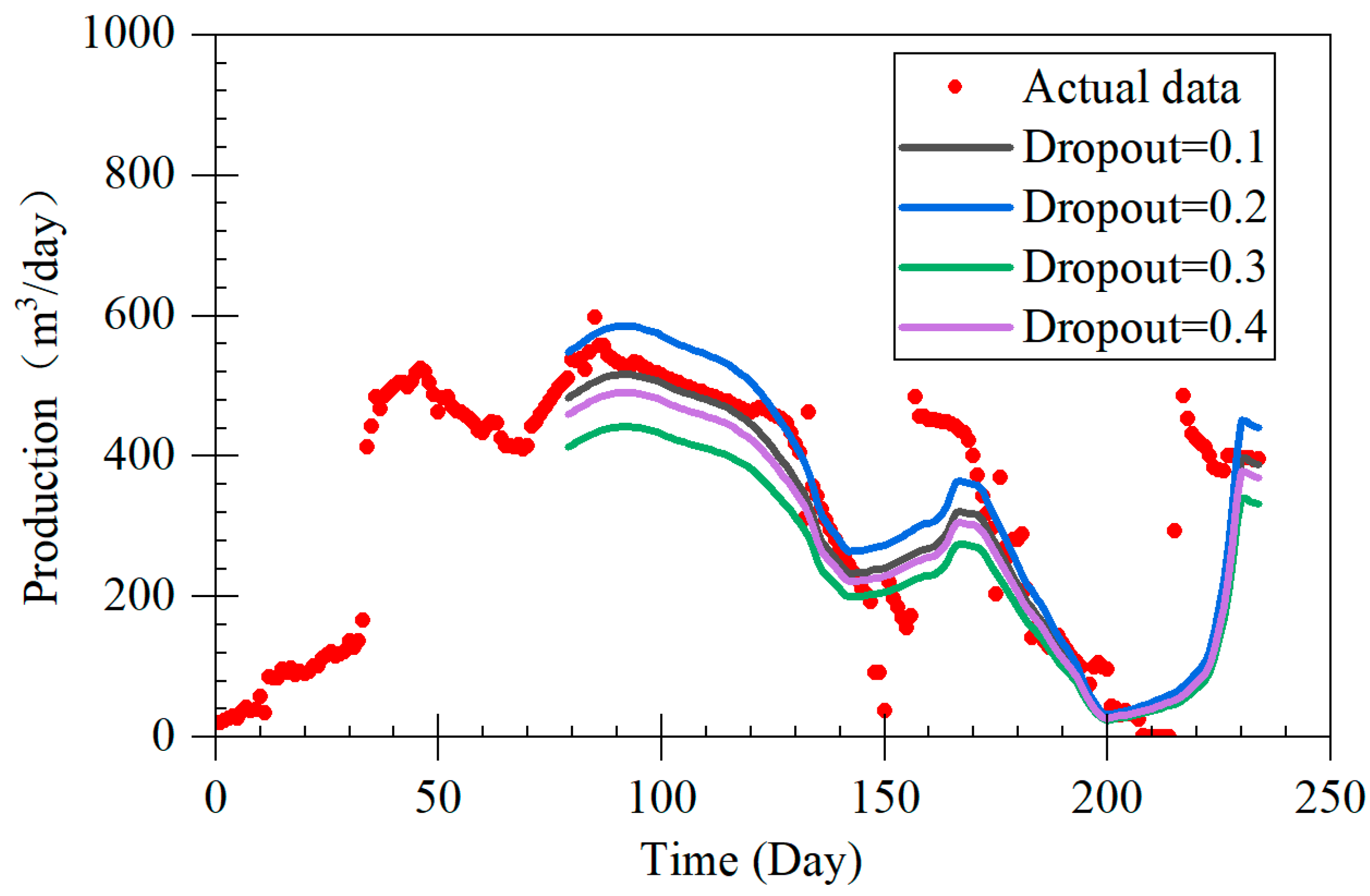
In the next phase, the data enter the Transformer encoder layers. These layers apply self-attention mechanisms, enabling the model to weigh the importance of different features and capture intricate dependencies within the sequence. This attention-based approach allows the model to focus on critical patterns, such as production peaks or declines, that span the entire time series. To mitigate overfitting, the output from the Transformer layers passes through a Dropout layer before a final fully connected layer generates the prediction. This architecture ensures that both short-term and long-term dependencies are effectively modeled, resulting in robust predictions of coal-bed methane production.

The model structure that integrates LSTM and Transformer combines the strengths of both to more effectively capture short-term dependencies, long-term dependencies, and global features in time-series data. The following sections will describe the entire model structure and computation process using paragraphs and formulas.

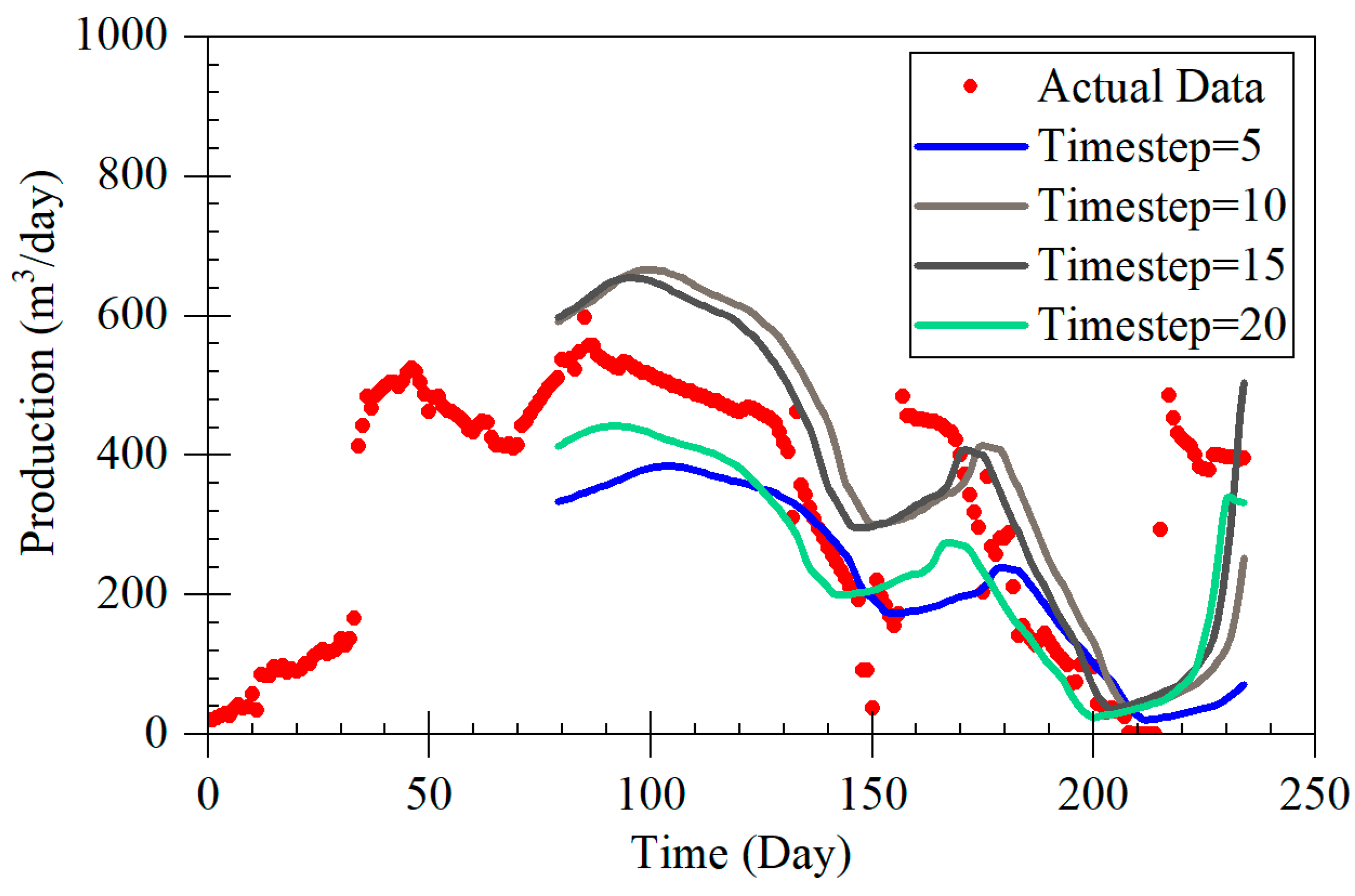
The input feature sequence $X\in {\mathbb{R}}^{B\times T\times D_{in}}$ is first passed through the LSTM model, where $B$ represents the batch size, $T$ is the number of time steps, and $D_{in}$ is the dimension of the input features. The LSTM functions by using its gating mechanisms to extract short-term and long-term dependency features from the input sequence. After processing by the LSTM, we obtain the hidden states at each time step $H_{LSTM}\in {\mathbb{R}}^{B\times T\times D_{LSTM}}$ and the cell state $C$:

$$H_{LSTM},C=LSTM\left(X\right)$$

(9)

The hidden states $H_{LSTM}$ contain the feature representations of the input sequence at each time step, where $D_{LSTM}$ represents the size of the LSTM hidden layer. These representations will be further processed.

To transform the output features of the LSTM into a feature dimension suitable for processing by the Transformer, we use a fully connected layer (linear layer). The function of the fully connected layer is to map the feature dimension $D_{LSTM}$ of the LSTM hidden states $H_{LSTM}$ to the feature dimension $D_{Transformer}$ required by the Transformer:

$$H_{\mathit{FC}1}=H_{\mathit{LSTM}}{W}_{\mathit{FC}1}+b_{\mathit{FC}1}$$

(10)

where $W_{FC1}\in {\mathbb{R}}^{D_{LSTM}\times D_{Transformer}}$ is the weight matrix and $b_{\mathit{FC}1}\in {\mathbb{R}}^{D_{Transformer}}$ is the bias vector. After passing through the fully connected layer, the output tensor shape becomes $H_{\mathit{FC}1}\in {\mathbb{R}}^{B\times T\times D_{Transformer}}$.

Next is the tensor shape adjustment, which aims to match the input format required by the Transformer layer. In PyTorch 3.1.2’s Transformer model, the time step must be the first dimension of the input. Therefore, we transform the dimensions of $H_{\mathit{FC}1}$:

$$H_{\mathit{Transformer} \mathit{input}}=\mathrm{permute}\left(H_{\mathit{FC}1}\right)$$

(11)

The tensor with adjusted dimensions is then fed into the Transformer layer. Through its attention mechanism, the Transformer layer can capture global feature relationships within the input sequence, especially handling long-distance dependencies. During the encoding process, we obtain the output of the Transformer $H_{\mathit{Transformer} \mathit{output}}\in {\mathbb{R}}^{B\times T\times D_{Transformer}}$:

$$H_{\mathit{Transformer} \mathit{output}}=\mathit{Transformer}\left(H_{\mathit{Transformer} \mathit{input}}\right)$$

(12)

This output retains the global features of each time step. Through multi-layer encoding and the attention mechanism, the Transformer can effectively learn the global context information of the sequence.

From the output of the Transformer layer, we typically select the hidden state of the last time step $H_{\mathit{Transformer} \mathit{output}} [-1]$ as the input, which is passed to the final fully connected layer to generate the final prediction:

$$H_{\mathit{final}}=H_{\mathit{Transformer} \mathit{output}}\left[-1\right]$$

(13)

Then, through a fully connected layer, the features are mapped to the output space to obtain the final prediction:

$$\widehat{y}=H_{final}{W}_{FC2}+b_{FC2}$$

(14)

The final output shape is $\widehat{y}$, representing the predicted values for each batch. Here, $W_{FC2}$ is the weight matrix, and $b_{FC2}$ is the bias vector.

By combining LSTM and Transformer, we leverage LSTM to extract short-term and long-term dependency features of the time series. These features are then mapped to a suitable dimension for the Transformer using a fully connected layer. The Transformer layer captures global feature relationships, and finally, the output passes through a fully connected layer to generate the final prediction. This combined model approach fully utilizes the advantages of both LSTM and Transformer, achieving a more profound modeling of time-series data.

2.4. Data Description

This study examines a CBM block in Yangquan, Shanxi. The specific location is shown in Figure 2. The mining area is located on the northeastern edge of the Qinshui coalfield, on the western side of the middle section of the Taihang Uplift. To the north of the mining area lies the Wutai block. It is situated on the eastern wing of the Qilu Arc and a series of graben-like polyphase structures in central Shanxi. The area forms a composite zone with the Taihang Uplift of the Neo-Cathaysian system and the latitudinal structural zone in central Shanxi, specifically the Yangqu–Yuxian east–west fold–fault zone. Additionally, it is positioned between the Shouyang–Xiluo meridional structure and the Taihang meridional structure. Production data from 21 representative wells were selected for analysis. The coal seam burial depths in the dataset vary significantly, ranging from 467 to 823 m. The reservoir is characterized by low permeability and pressure. The data cover the period from post-fracturing operations to the end of production.

The sample set is divided into two subsets based on the different fracturing operation times and production dates, comprising 9 and 12 wells, respectively. The interval between fracturing operations within each subset does not exceed three months. Due to varying well conditions, the production periods can differ by up to 110 days.

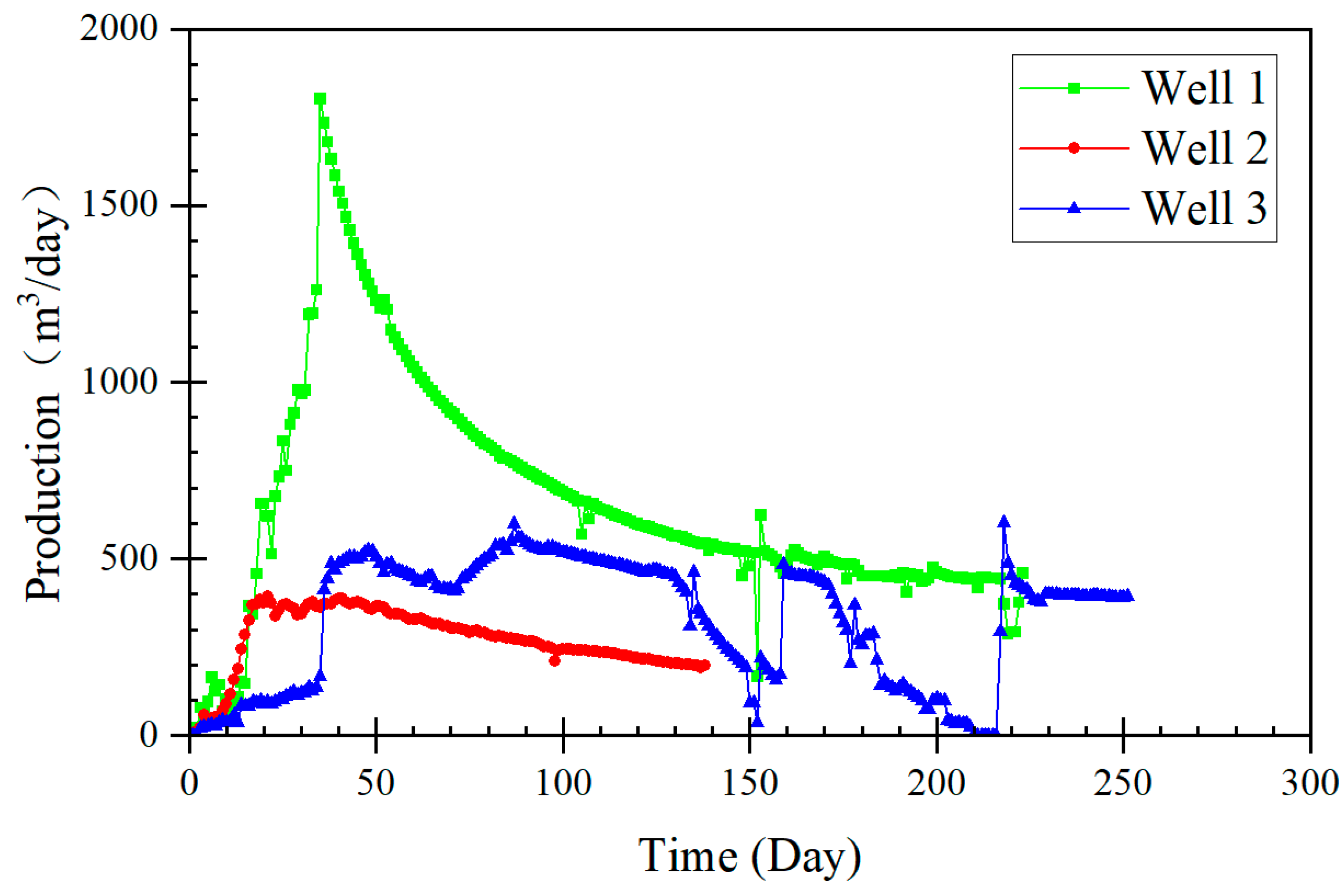
Due to the influence of geological conditions and fracturing operations, CBM wells’ final production and production variations with similar production dates and gas-bearing layers can vary significantly. As Figure 3 illustrates, CBM wells can be categorized into three types based on their production volume and variation: declining, stable, and fluctuating. Well 1 is a typical example of a declining CBM well. It has a gas-bearing layer with a high gas content, effective fracturing results, high permeability, and low water content. During the extraction process, no equipment failures occurred, and there were no artificial restrictions from the production stage onward. Its production curve can be divided into three stages: rapid increase in production, noticeable decline, and stable production. This type of CBM well is ideal but often rare.

The primary reasons for the significant difference between actual production curves and ideal curves can be attributed to two main factors. One is long-term factors such as reservoir geology. For example, if the coal seam has poor permeability, gas will have difficulty migrating from within the coal seam to the wellbore, even after fracturing operations. Similarly, high water content in the coal seam, complex geological structures, low gas content, and formation stress causing fracture closure can also lead to variations in gas production. The surrounding rock’s poor sealing properties can result in wells like Well 2, which, despite overall stability, have low gas production. In severe cases, gas production may stop or not occur shortly after starting.

Another type of factor is short-term influences, which include inter-well interference caused by fracturing operations in adjacent wells, human interventions in production through extraction plans, and sudden issues with extraction equipment. These influences can immediately and significantly impact production. For instance, the production curve of Well 3 shows high overall output with frequent sharp increases or decreases in daily production. Identifying the reasons for these abrupt changes in production and preventing and addressing similar issues has been a critical focus in CBM development. Wells affected by these short-term influences constitute the majority of cases.

2.5. Data Preprocess

Data preprocessing plays a pivotal role in enhancing model performance and prediction accuracy. To ensure high data quality and minimize interference, this study implemented a comprehensive series of preprocessing steps, including normalization, noise management, and missing data imputation. Data points where production remained below 100 m³ for more than 20 consecutive days were removed, ensuring completeness while filtering abnormal values.

To address the variability in scales and ranges among feature values, the Min-Max normalization method was utilized, mapping all features to the range [0, 1]. The normalization formula used is

$$x^{\prime }={\displaystyle \frac{x-\mathit{min}\left(x\right)}{\mathit{max}\left(x\right)-\mathit{min}\left(x\right)}}$$

(15)

Here, $x$ represents the original feature value, while $min\left(x\right)$ and $max\left(x\right)$ denote the minimum and maximum values of the feature, respectively. This method reduces discrepancies in feature scales, preventing any single feature from disproportionately influencing the model during training. Additionally, normalization helps accelerate model convergence by standardizing input values.

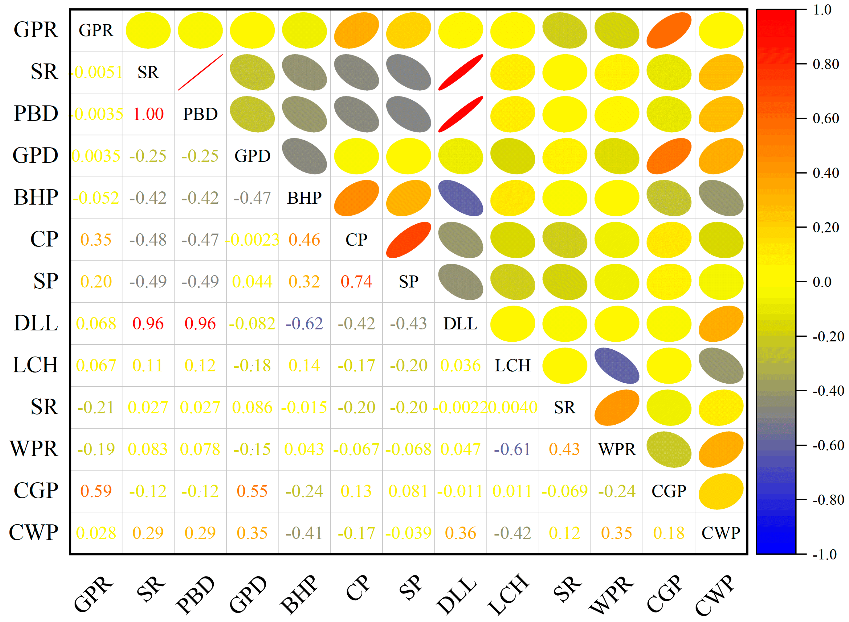
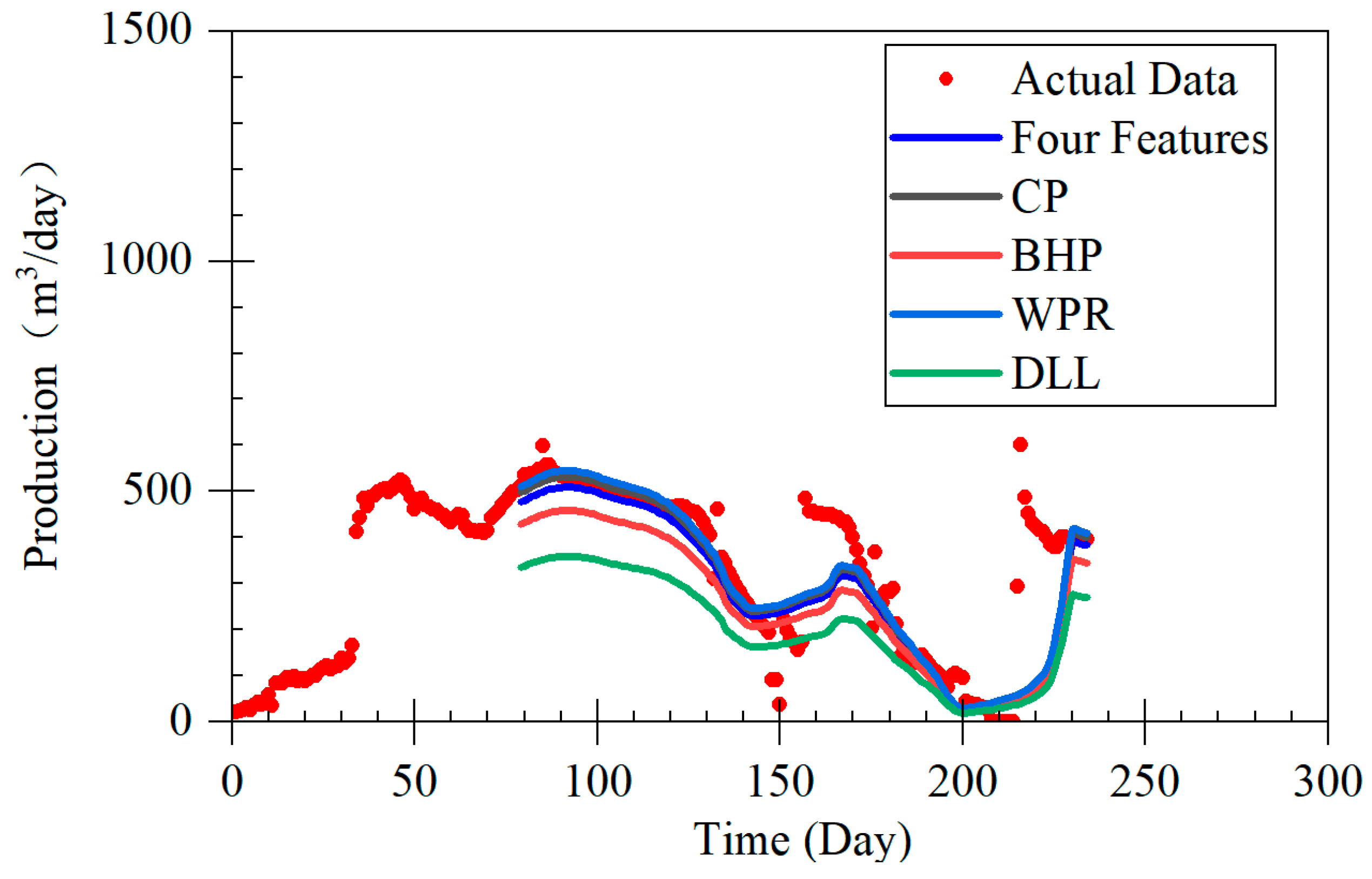
Noise in the data, particularly zero-point data and outliers, was also addressed. Zero-point data, often caused by equipment failures or transmission errors, can harm model performance. Data with excessive zero values or prolonged consecutive zeros were removed using thresholds. After removing noise, GPD shows a relatively weak positive correlation with other production parameters (Figure 4), and the correlations between other features are also not particularly pronounced. Considering the correlation between the features and the significance of the features themselves, the model selected bottomhole pressure (BHP), casing pressure (CP), water production rate (WPR), and dynamic liquid level (DLL) as input features.

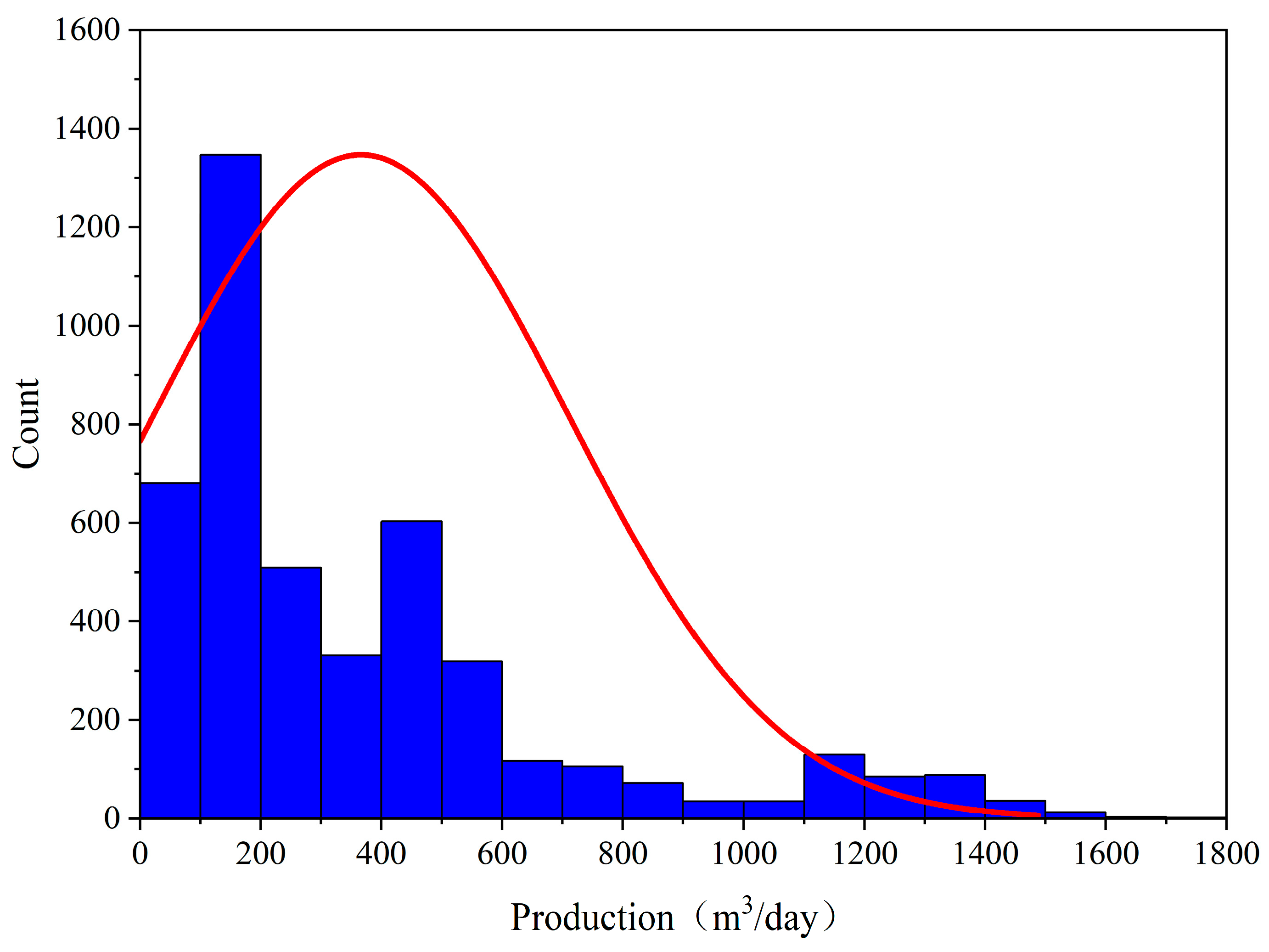
The data were derived from two datasets, including 3078 samples from primary fracturing and 3545 samples from secondary fracturing. After removing outliers, 4512 data points were retained (Figure 5). The production data exhibit a clear right-skewed distribution (positive skewness), with most samples concentrated in the lower production range, while high-production samples are relatively rare. This distribution characteristic is common in coalbed methane production and reflects the resource limitations and technological impacts on well productivity.

Missing data were handled based on their proportion. For features with less than 5% missing values, linear interpolation or time-series mean methods were used. For higher proportions, the affected time periods were excluded to avoid errors. Inconsistent sensor sampling frequencies were aligned and resampled to a daily interval, and interpolation filled gaps to ensure temporal consistency.

3. Results

This section compares the performance of the LSTM-A, LSTM, exponential, and harmonic models in predicting the production of different types of CBM wells. The evaluation metrics used include MAE, RMSE, and R². After determining the strengths and weaknesses of the LSTM-A model relative to the other models, the model optimization process regarding feature selection and parameter tuning is analyzed.

To assess the model’s performance, several key metrics are used: MAE, RMSE, and R² score. The MAE is calculated as

$$MAE={\displaystyle \frac{1}{n}}\sum _{i=1}^n|X_i-Y_i|$$

(16)

where $X_i$ is the actual value, $Y_i$ is the predicted value, and $n$ is the number of predictions. The RMSE can be expressed as

$$RMSE=\sqrt{{\displaystyle \frac{1}{n}}\sum _{i=1}^n(X_i-Y_i{)}^2}$$

(17)

The R² score is computed as

$$R^2=1-{\displaystyle \frac{\sum _{i=1}^n(X_i-Y_i{)}^2}{\sum _{i=1}^n(X_i-\overline{X}{)}^2}}$$

(18)

where $\overline{X}$ is the mean of the actual values. These metrics provide a comprehensive evaluation of the model’s predictive performance, with lower MAE and RMSE values indicating higher accuracy and a higher R² score, indicating better model fit.

3.1. Model Optimization

The hyperparameter settings of the model are key to model tuning [45]. In order to improve the prediction accuracy of the model, reduce the training time, and prevent overfitting, we discuss the effects of feature selection, Dropout rate, time step, and layer number on the prediction effect and apply them to optimize the prediction model. The remaining hyperparameters are detailed in

Table 1. LSTM-A model architecture, developed in Python 3.12.

Parameters	Values
LSTM Layers	2
LSTM Hidden Size	128
Transformer Layers (Encoder)	6
Transformer Layers (Decoder)	6
Transformer Hidden Size	128
Number of Attention Heads	8
Dropout Rate	0.3
Final Output Size	1

. The dataset contains a total of 4512 data points. Considering the varying production cycles of individual wells, the test set was not allocated strictly by proportion. Overall, approximately 90% of the data were allocated to the training set, and about 10% were allocated to the test set. Well 3 is a complex situation. This is consistent with the pattern of most CBM wells and is a suitable candidate for validation.

3.1.1. Feature Selection

Selecting different features significantly impacts the prediction results in Figure 6. When using casing pressure and water production as features for prediction, the main trends and variations in production can be accurately reflected, resulting in the most accurate predictions.

The MAE obtained using CP as a feature is the lowest among all prediction results (

Table 2. Prediction accuracy evaluation of different features.

Model	Four Features	CP	BHP	WPR	DLL
MAE	71.03	63.64	93.53	63.66	142.85
RMSE	115.17	111.50	129.09	110.20	171.74
R2	0.56	0.58	0.44	0.59	0.01

). The RMSE obtained using WPR is the lowest among all prediction results. Additionally, the prediction result using WPR as a feature yields the highest R² value. The prediction results using BHP as a feature are average. Finally, the prediction results obtained using the above four parameters as features have an MAE of 71.03, an RMSE of 115.17, and an R² of 0.56, accurately reflecting actual production conditions. When using all four features, the negative impact of high-dimensional data on the model is minimal and exhibits good stability.

3.1.2. Dropout Rate

Dropout is a regularization technique that randomly drops a certain percentage of neurons during training to prevent the model from overfitting (Figure 7). The model shows the best prediction performance at a Dropout rate of 0.1. When the Dropout rate increases to 0.2, MAE and RMSE increase slightly (

Table 3. Prediction accuracy evaluation of different Dropout rates.

Dropout Rate	0.1	0.2	0.3	0.4
MAE	68.02	70.08	101.47	79.09
RMSE	113.86	110.19	135.13	119.40
R2	0.57	0.59	0.39	0.52

).

However, a further increase in the Dropout rate to 0.3 results in a marked deterioration in model performance. At a Dropout rate of 0.4, the predictive performance is still worse than at Dropout rates of 0.1 and 0.2. A lower Dropout rate (0.1 or 0.2) is more favorable.

3.1.3. Time Step

The time step determines the number of past time points the model can consider when predicting the current output. As shown in Figure 8, the model’s fit to the actual data is poor at a time step of 5, especially in the early stages of prediction, where the model fails to capture the fluctuations in production accurately. With a time step of 10, the model’s performance improves but still exhibits significant deviations. The performance at a time step of 15 is better than that of the previous two. Beyond the 100-day mark, the model can better track the production trend. The curve at a time step of 20 shows a trend more closely aligned with actual production, making this time step the best-performing one. Overall, the longer the time step, the more accurate the prediction becomes. However, to prevent issues such as over-smoothing of the model and loss of detailed information, as well as to reduce the risk of overfitting, the time step will no longer be increased. The model uses 20 time steps to make predictions.

As the time step increases, the R² value gradually rises, reaching 0.39 at a time step of 20, indicating an enhancement in the model’s explanatory power of the data (

Table 4. Prediction accuracy evaluation of different time steps.

Time Step	5	10	15	20
MAE	137.73	144.14	115.21	101.47
RMSE	181.27	167.50	141.91	135.13
R2	−0.10	0.06	0.32	0.39

). The gradual decrease in MAE and RMSE also indicates that the longer the time step, the stronger the model’s prediction ability.

3.1.4. Layer

The number of layers determines the complexity and expressiveness of the model. More layers typically capture more complex patterns in the data, but they may also lead to overfitting. The overall trend in the one-layer model aligns well with the actual data (Figure 9). The two-layer model significantly underestimates daily production at the beginning of the forecast. The three-layer model performs slightly better than the two-layer model, but some areas still have significant errors. The four-layer model shows the closest trend to the actual data in the figure. During significant fluctuations, the model almost wholly follows the changes in actual production. It has the lowest MAE (64.49) and the highest R² (0.60) (

Table 5. Prediction accuracy evaluation of different layers.

Model	1 Layer	2 Layers	3 Layers	4 Layers
MAE	65.86	101.47	83.91	64.49
RMSE	109.45	135.13	122.36	109.57
R2	0.60	0.39	0.50	0.60

).

Several characteristics, including casing pressure and water production, can be improved by adjusting the parameters. The model performed best at loss rates of 0.1 and 0.2. Longer time steps improved performance and reduced the MAE and RMSE, while one- and four-zone configurations provided the best accuracy. These results are applied to different well data in the next section.

3.2. Field Application

3.2.1. Rapid Decline Prediction

The actual daily production data for the CBM show a clear downward trend (Figure 10). Among the two conventional production decline curves, the exponential model fits the actual data poorly, mainly underestimating the production in the later stages. The harmonic model, while less accurate in predicting the early trend than the exponential model, performs better in the last stages, only slightly underestimating the production. Li–Horne’s model grossly overestimates future production.

The LSTM model exhibits noticeable volatility in its predictions from the beginning, with the primary source of error being significant fluctuations. However, it remains relatively accurate over the long term (Figure 11). All models use a certain period of prior data as the training set. The LSTM-A model effectively corrects the volatility error of the LSTM model, allowing for long-term tracking of the actual data trend (

Table 6. Prediction accuracy evaluation of LSTM-A model with LSTM, Li–Horne model, exponential model, and harmonic model in production decline stage for Well 1.

Model	LSTM	LSTM-A	Exponential Model	Harmonic Model	Li–Horne Model
MAE	57.51	18.27	229.93	76.88	258.17
RMSE	74.70	37.98	242.30	84.97	268.80
R2	0.17	0.79	−7.70	−0.07	−11.51

).

3.2.2. Stable Production Prediction

Figure 12 shows the predictive performance of the LSTM-A model compared to the LSTM, exponential model, harmonic model, and Li–Horne model during a stable production decline phase. The CBM production data remain stable and gradually decline after a certain period. Both the exponential and harmonic models in the ARPS model performed poorly, so the Li–Horne model was added as a comparison; the exponential model performed well during the stable production phase but significantly overestimated production in the later stages (

Table 7. Prediction accuracy evaluation of LSTM-A model with LSTM, Li–Horne model, exponential model, and harmonic model in production decline stage for Well 2.

Model	LSTM	LSTM-A	Exponential Model	Harmonic Model	Li–Horne Model
MAE	21.63	7.75	67.17	100.34	33.02
RMSE	25.74	9.72	71.40	100.54	39.01
R2	0.41	0.92	−3.52	−7.96	−0.349

). The harmonic model, which predicted an initial decline followed by stable production, completely contradicted the actual production trend. The Li–Horne model outperformed the first two but still overestimated the yield.

The LSTM model’s overall predictions are close to the actual values, slightly underestimating production in the early phase and overestimating it in the later phase, with the actual decline being more pronounced than the model predicts (Figure 13). The LSTM-A model’s overall predictive trend is very close to the actual values, with an R² value reaching 0.92, indicating a solid alignment with the actual data.

Overall, the LSTM-A model demonstrates a higher prediction accuracy than the LSTM model, especially in tracking the decline phase of the actual production data. The LSTM model, while following the trend, shows more significant prediction errors and fluctuations.

3.2.3. Fluctuating Production Prediction

Figure 14 illustrates the prediction results of two machine learning models for fluctuating CBM production. The actual data exhibit considerable variability and multiple peaks during the production period. It is evident that conventional production decline curve models, including the exponential and harmonic models, cannot predict this type of production decline curve.

The LSTM model performs poorly in this prediction. Although the final predicted production amount is close to the actual value, the trend significantly deviates from the actual data (Figure 15). In comparison, the LSTM-A model demonstrates better consistency with the peaks and troughs of actual production data, with the R² improving from −1.04 (LSTM) to 0.56.

4. Discussion

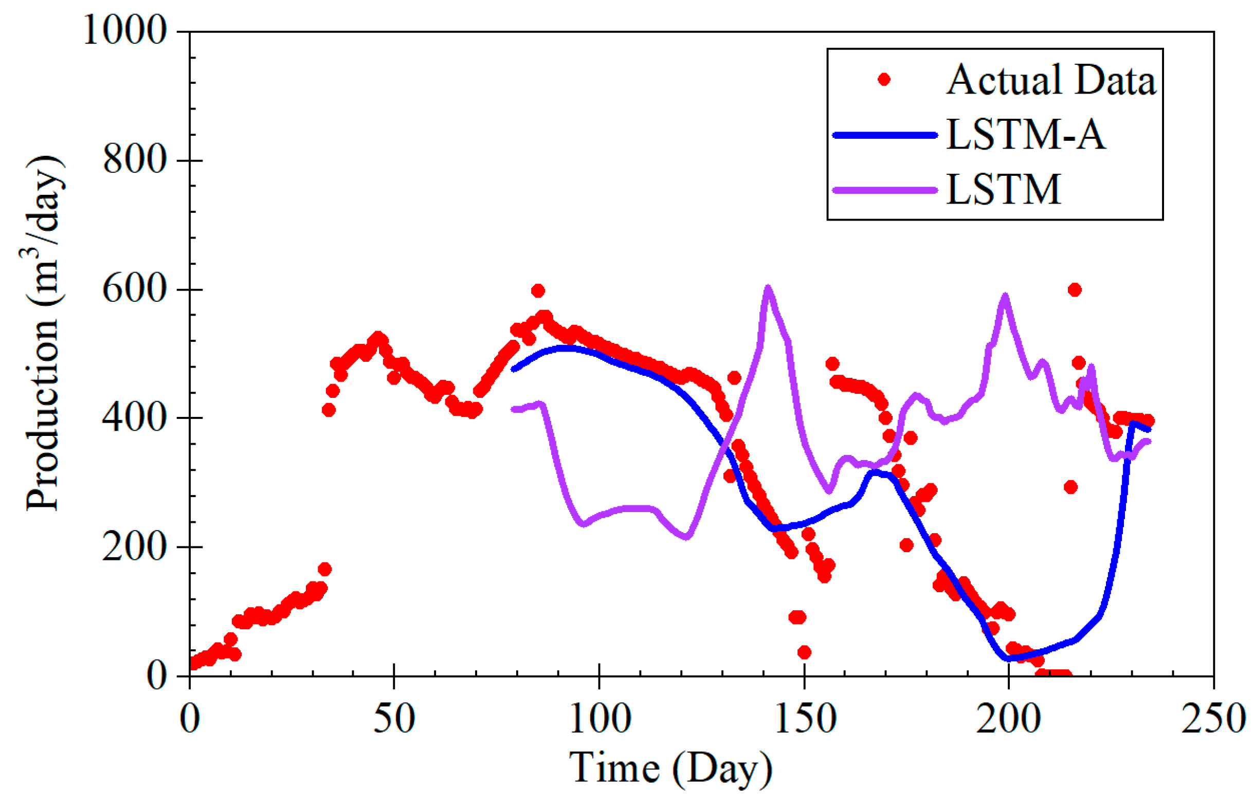
The LSTM-A model proposed in this study demonstrates significant advantages in forecasting coalbed methane (CBM) production, particularly across different production stages, including rapid decline, stable production, and fluctuating production. By combining long short-term memory (LSTM) networks with the attention mechanism of the Transformer architecture, the LSTM-A model effectively captures both short- and long-term dependencies in time-series data, leading to a marked improvement in prediction accuracy. When compared with traditional Decline Curve Analysis (DCA) models, the LSTM-A model outperforms in all production phases, especially in stages with greater production fluctuations.

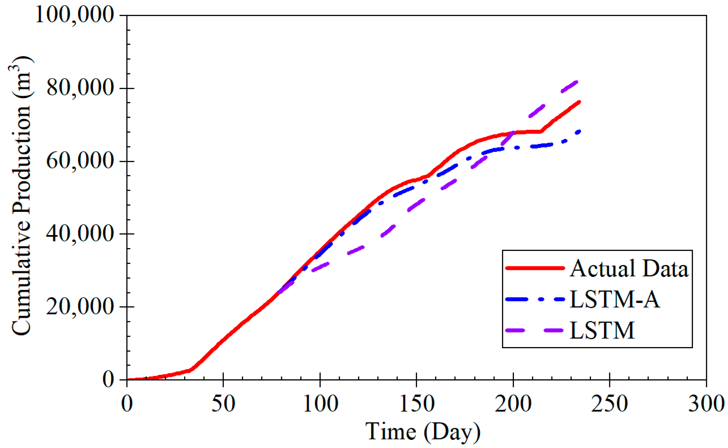
The results of this study demonstrate the effectiveness of the LSTM-A model in predicting CBM production, particularly in comparison with traditional decline curve models and the LSTM model alone [46]. The LSTM-A model showed superior performance in short-term and long-term production predictions across various production stages—declining, stable, and fluctuating.

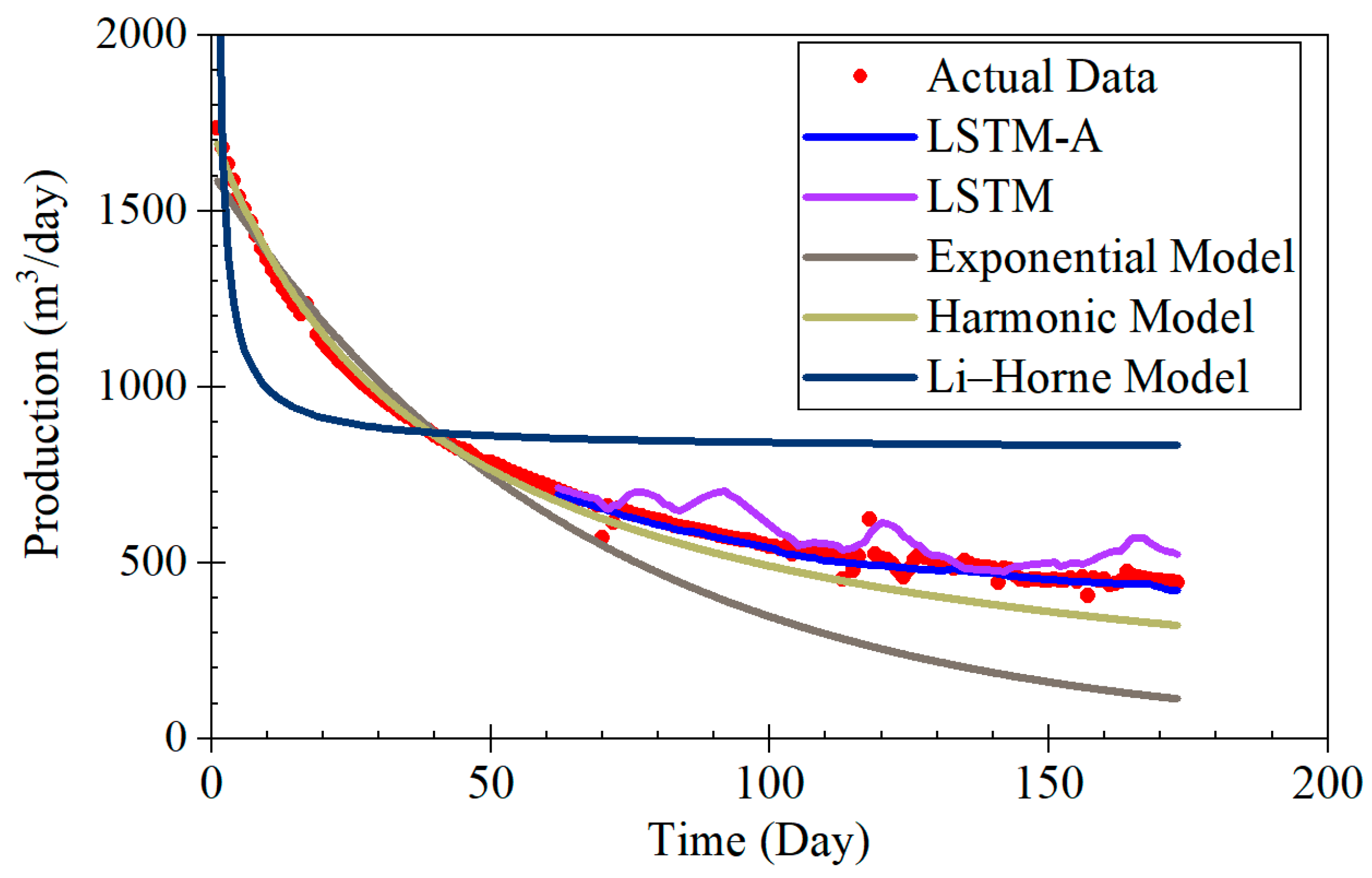
During the rapid decline phase, the LSTM-A significantly outperformed traditional exponential and harmonic models, which tended to underestimate production, especially in later stages. While the LSTM model also provided accurate predictions, it displayed some volatility that was effectively smoothed by incorporating the attention mechanism in the LSTM-A.

Compared to traditional prediction methods, such as DCA and other numerical simulation methods, the approach proposed in this study demonstrates clear advantages. Traditional methods often rely on empirical formulas or simplified physical models, which struggle to accurately capture the complexity of CBM reservoirs, particularly in dynamic and unconventional environments. While DCA models perform well under steady-state conditions, they cannot adapt to rapidly changing production data, making them unsuitable for real-time predictions. In contrast, the method proposed in this study effectively handles time-series data and dynamically adjusts to evolving reservoir conditions, providing more accurate predictions.

Although the DNN model demonstrates a high coefficient of determination (R² = 0.923) [47], it mainly relies on static data, limiting its ability to model the dynamic features of CBM production. By integrating the attention mechanism, the method proposed here can prioritize important features, enhancing its ability to capture long-term dependencies and abrupt changes in production, a capability that is often overlooked by other machine learning models.

The hybrid method that combines convolutional neural networks (CNNs) and LSTM shares similarities with the approach presented in this study, particularly in feature extraction and time-series modeling [36]. However, the attention mechanism in this study further optimizes the feature weighting process by allowing the model to focus on the most important time steps, improving prediction accuracy. This enables the method to be more adaptable to different well conditions and production scenarios, while the hybrid models in the literature lack this optimization layer.

Wei Xiaoyi successfully applied the LSTM model to predict CBM production and based their model on geological data [48]; they typically only used static factors such as coal seam depth and permeability. In contrast, the method presented here integrates both geological data and dynamic production data (such as pressure and gas production rates), offering a more comprehensive approach to CBM production forecasting. This integrated approach allows for more accurate and timely predictions, as it considers not only geological features but also the continuously changing production conditions.

The method proposed in this study, by integrating dynamic and static data and providing stronger adaptability through the attention mechanism, exhibits better computational stability and prediction accuracy, demonstrating superior performance compared to existing CBM prediction models. It presents a promising tool for real-time, large-scale applications in CBM production forecasting.

Despite its advantages, the LSTM-A does have some limitations, particularly when predicting highly volatile production data. Future research could explore incorporating additional features or developing hybrid models that combine strengths from different machine learning approaches.

Although the model proposed in this study demonstrates promising performance in coalbed methane (CBM) production forecasting, there is still room for improvement. Future research can explore several directions. First, while the model effectively captures dynamic changes in production data, it may still face challenges in extreme conditions, such as in areas with complex geological environments. To further enhance the model’s diversity and stability, more types of deep learning models, such as graph neural networks or generative adversarial networks, could be integrated to improve its predictive ability in high-variance or unknown production patterns. Secondly, although this study combined geological data and dynamic production data, future research could incorporate additional data sources, such as climate change, socio-economic factors, or multi-scale geological models, to more comprehensively assess the production potential of CBM.

Moreover, as production environments evolve rapidly, real-time data stream-based forecasting systems will be increasingly important. Future studies could explore online learning methods that enable the model to adjust its predictions in real time, better addressing uncertainties in actual production, especially over long production cycles. Furthermore, the method presented here could be expanded to other types of unconventional energy, such as shale gas and tight gas. Given the similarities in geological characteristics and production data between these energy sources and CBM, the proposed model could have broader applicability. Finally, although deep learning models have significantly improved prediction accuracy, their “black box” nature remains a challenge. Future research could focus on enhancing model interpretability, for example, through visualization techniques or attention mechanisms within the model, to help users better understand which factors contribute the most to the prediction results.

5. Conclusions

The LSTM-A model proposed in this study effectively integrates geological data and well cluster features. The model can accurately predict future trends by utilizing time-series attributes closely related to production. The following conclusions were drawn:

(1)

The LSTM-A model demonstrates superior performance in predicting CBM production, particularly during the rapid decline and stable production phases, outperforming traditional ARPS, Li–Horne, and LSTM models and proving its effectiveness across various production curve types.

(2)

The combination of Transformer and LSTM architectures enables the LSTM-A model to more effectively analyze the temporal complexity of CBM extraction, significantly improving the R² score from 0.17 (LSTM) to 0.79 (LSTM-A) and enhancing the model’s explanatory power.

(3)

By optimizing the key parameters, such as feature selection, Dropout rate, time step, and the number of layers, the LSTM-A model effectively balances prediction accuracy and training efficiency, making it well suited for diverse CBM production scenarios.

(4)

The incorporation of certain engineering parameters (CP, BHP, WPR, DLL) as features has significantly improved the predictive capability of the model. These engineering parameters offer advantages over geological parameters, such as being easier to obtain, lower in cost, higher in accuracy, easier to standardize, and more intuitively impactful.

(5)

The LSTM-A model successfully captures the periodicity and regression characteristics of fluctuating production data. It is capable of handling short-term production fluctuations and long-term trend changes.