Analysis and Control Parameters Optimization of Wind Turbines Participating in Power System Primary Frequency Regulation with the Consideration of Secondary Frequency Drop

Abstract

With the increasing integration of wind energy into power systems, maintaining frequency stability has become a significant challenge. To address the issue of secondary frequency drop caused by wind turbines exiting the primary frequency regulation of power systems, this paper presents a control parameters optimization method of wind turbines participating in power system primary frequency regulation. Initially, with the assumption of constant wind speed and linearization of the wind power coefficient, the relationship between the mechanical power and rotor speed of the wind turbines is established. Subsequently, the primary frequency regulation component of wind turbines is integrated into the classical system frequency response (SFR) model, accounting for the effects of exiting time and rotor speed variations. Following this, the dynamic frequency of the power system is computed with the modified SFR model, and the time domain expressions for both primary and secondary frequency drops are derived. Furthermore, an optimization model for the control parameters of wind turbines participating in primary frequency regulation is developed, aiming to minimize the values both of primary and secondary frequency drops. Finally, a case study is constructed to validate the efficacy of the proposed method. The results demonstrate that the optimization method introduced in this paper significantly enhances the dynamic characteristics of the system frequency.

1. Introduction

Driven by the global energy transition, renewable energy sources, particularly wind and photovoltaic power, are progressively displacing conventional power generation on an unprecedented scale worldwide. As of the end of 2024, China’s installed capacity of new energy power generation, predominantly consisting of wind and photovoltaic power, had reached 1.45 billion kW, marking a historic milestone by surpassing thermal power capacity for the first time, while demonstrating accelerated growth in the renewable energy sector. The integration of large-scale wind power, photovoltaic power, and other renewable energy sources into the power system via power electronic converters has led to the gradual displacement of conventional synchronous generator units. This transition has resulted in a reduction in overall power system inertia, a decline in primary frequency regulation capability, and a deterioration of dynamic frequency characteristics. As a consequence, the power system’s resilience to power disturbances has been significantly compromised, heightening the risk of frequency instability [1].

Grid-connected wind power and photovoltaic power should have active primary frequency regulation ability with the increasing penetration rate of new energy [2]. Wind turbines participate in the primary frequency regulation of a power system by utilizing the rapid power modulation capability of electronic converters. The control strategies primarily include virtual inertia control and droop control [3]. Virtual inertia control emulates the inertial response of conventional synchronous generator units, while droop control replicates the governor characteristics of these traditional units [4,5]. Concurrently, both pitch angle control and de-loaded power tracking control are employed to supply power reserve for wind turbines’ primary frequency regulation [6]. Nevertheless, these methods lead to decreased wind energy utilization efficiency, thereby exhibiting economic drawbacks.

The release of more than half of the rotor’s kinetic energy by wind turbines would result in improved economic performance and greater potential in frequency regulation [7]. However, most existing studies have failed to account for the dynamic changes in wind turbine rotor speed and kinetic energy during primary frequency regulation. The release of kinetic energy from wind turbines results in a reduction in rotor speed and mechanical power [8], which imposes temporal constraints on wind turbines’ engagement in primary frequency regulation control. When wind turbines exit primary frequency regulation control due to the rotor speed decline, a new active power deficit will be caused in the power system, resulting in the secondary frequency drop and affecting the frequency stability of power system [9]. The previously mentioned problem can be mitigated by implementing optimal control strategies for parameters adjustment and power regulation in wind turbines engaged in primary frequency regulation. These approaches are designed to mitigate the power deficit resulting from wind turbines’ disengagement from primary frequency regulation. The specific measures comprise (1) the enhancement of the power–rotor speed characteristics during primary frequency regulation [10,11,12]; (2) optimization of primary frequency regulation control parameters based on disturbance power magnitude to prevent excessive release of rotor kinetic energy [13,14,15]; and (3) implementation of advanced control strategies, including (i) nonlinear droop control with adaptive parameter adjustment according to rotor speed variations [16], (ii) utilization of energy state indices for rotor kinetic energy quantification and corresponding parameter optimization [17], and (iii) coordinated operation with energy storage systems to maintain continuous frequency regulation capability [18,19,20].

In contrast to previous studies, this paper focuses on the optimization of primary frequency regulation control parameters for wind turbines, with particular attention to the secondary frequency drop phenomenon. Unlike the previous studies, we integrate both wind turbine inertia control and droop control into the system frequency response (SFR) model. This dual-control integration enables a more comprehensive analysis of the dynamic relationship between wind turbine output power, rotor speed, and system frequency characteristics. The modified SFR model provides a more precise assessment of rotor kinetic energy’s role in frequency regulation processes. Furthermore, we introduce a novel consideration of wind turbine exiting time into the SFR model, allowing for systematic simulation of its impact on secondary frequency drop characteristics. These methodological advancements in the modified SFR model offer unprecedented insights into the kinetic energy release dynamics and their subsequent effects on secondary frequency drop that have been insufficiently addressed in existing research paradigms.

The primary objective of this paper is to develop and optimize the primary frequency regulation control parameters for wind turbines, with a specific focus on minimizing both primary and secondary frequency drops. An optimization approach is proposed to adjust the control parameters of wind turbines in such a way that both primary and secondary frequency drop values are minimized, resulting in a more efficiently viable primary frequency regulation process. Thus, the optimization model presented shifts the focus from merely delaying the secondary frequency drop to integrating it into the optimization process of primary frequency regulation. The effectiveness of wind turbine participation in power system frequency regulation can be enhanced.

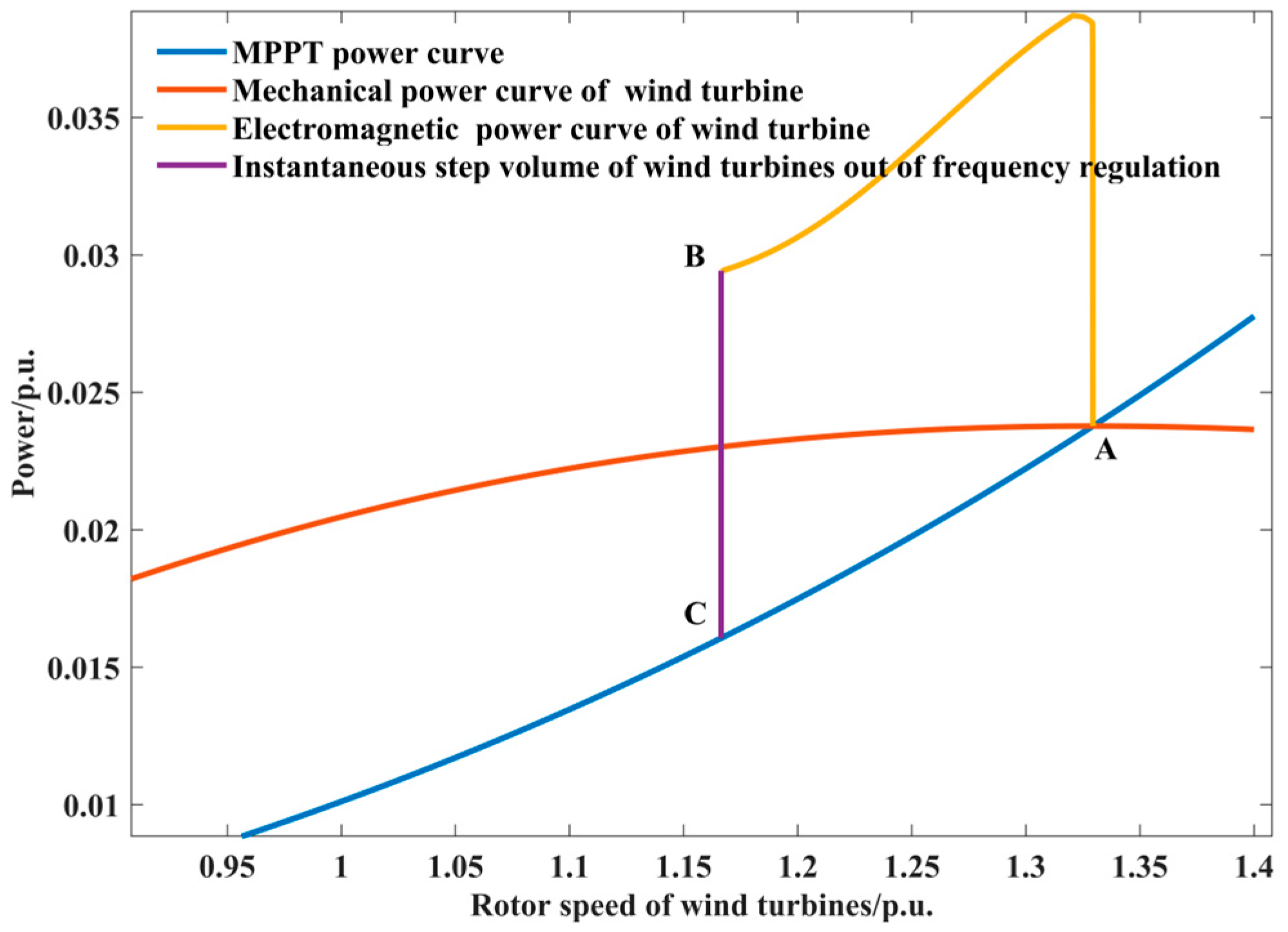
2. Analysis of the Influence of the Wind Turbine Rotor Speed on Mechanical Power

The wind turbine mechanical power is affected by two key factors: the wind power coefficient and the input wind power. Assuming that there are n_w wind turbines participating in the primary frequency regulation, the total mechanical power of the wind turbines can be expressed as follows:

$$P_{\mathrm{m}}=C_{\mathrm{p}}·P_{\mathrm{v}}·n_{\mathrm{w}}$$

(1)

where P_m is the total mechanical power of wind turbines; C_p is the wind power coefficient; and P_v is the input wind power of single wind turbine.

The expression of P_v is

$$P_v={\displaystyle \frac{1}{2}}\rho S_{\mathrm{w}}{v}^3$$

(2)

where ρ is the air density; S_w is the wind turbine blade swept area; and v is the wind speed.

The wind power coefficient is affected by the pitch angle and tip speed ratio [21]. In the absence of pitch angle control, the wind turbine power coefficient C_p can be expressed in terms of the tip speed ratio λ as follows:

$$C_{\mathrm{p}}(\lambda )=C_1\left[C_2\left({\displaystyle \frac{1}{\lambda }}-0.035\right)-C_3\right]·\exp \left[-C_4\left({\displaystyle \frac{1}{\lambda }}-0.035\right)\right]+C_5\lambda$$

(3)

where C₁~C₅ are coefficients related to the wind turbine power coefficient characteristics; λ is the tip speed ratio.

The wind turbine tip speed ratio can be expressed as follows:

$$\lambda ={\displaystyle \frac{R_{\mathrm{w}}{\omega }_{\mathrm{r}}}{v}}$$

(4)

where R_w is the wind turbine blade radius. ω_r is the wind turbine rotor speed.

The variations in wind turbine rotor speed and wind speed lead to a corresponding variation in tip speed ratio. The small signal increment of C_p is

$$\Delta C_{\mathrm{p}}({\omega }_r)={\displaystyle \frac{0.29\pi R_w}{V_w}}·\cos ({\displaystyle \frac{\pi R{\omega }_{r0}}{15V_w}}-{\displaystyle \frac{\pi }{5}})\Delta {\omega }_r$$

(5)

where λ₀ is the initial tip speed ratio.

In the context of the primary frequency regulation of wind turbines, the influence of wind speed change is often overlooked. By substituting Equations (4) and (5) into Equation (1), the mechanical power change in the wind turbines can be determined:

$$\Delta P_{\mathrm{m}}=C_{\mathrm{p}}^{\prime }({\omega }_{r0})·P_v·n_{\mathrm{w}}·\Delta {\omega }_{\mathrm{r}}=K_{\mathrm{cp}}·\Delta {\omega }_{\mathrm{r}}$$

(6)

where K_cp is the ratio between the mechanical power change and rotor speed change in wind turbines. Δω_r is the rotor speed change.

3. Analysis of Wind Turbine Rotor Motion Status When Participating in Frequency Regulation

Figure 1 illustrates the wind turbine power–rotor speed curves participating in the primary frequency regulation. In the absence of de-loaded power tracking control, the initial operating point of the wind turbine is point A of the intersection between the mechanical power curve and the maximum power point tracking (MPPT) curve. As the power system load increases, the wind turbine generates additional electromagnetic power in accordance with the control strategy. Concurrently, the electromagnetic power exceeds the mechanical power, resulting in a reduction in rotor speed and a shift in the operating point from point A to point B. When the wind turbine quits the primary frequency regulation, the electromagnetic power abruptly declines to the MPPT power corresponding to the current rotor speed, resulting in the wind turbine transitioning from operating point B to point C. At point C, the mechanical power exceeds the electromagnetic power, the wind turbine rotor speed increases, and the operating point gradually ascends to point A along the curve CA.

Considering the interaction between system frequency and the wind turbine’s active power, as well as the influence of the wind turbine’s participation in primary frequency regulation on the wind turbine rotor speed, the system frequency response model, which incorporates the wind turbine’s primary frequency regulation link introduced into the SFR model, is illustrated in Figure 2.

In this figure, H is the inertia constant of the conventional generator unit. D is the damping coefficient. K_m is the mechanical power gain coefficient. R is the governor drop coefficient. F_H is the fraction of total power generated by the high-pressure turbine. T_R is the reheater time constant. P_d is the disturbance power caused by load changing. The value greater than zero indicates a decrease in load, while the value less than zero indicates an increase in load. Δω is rotor speed variation in the traditional generator rotor. H_w is the inertia time constant of the wind turbine under the equivalent value of a single unit. K_df is the droop control coefficient. K_pf is the virtual inertia control coefficient. ΔP_e is the variation in electromagnetic power of the wind turbine. The value less than zero indicates an increase in electromagnetic power, while the value greater than zero indicates a decrease. ΔP_m is the variation in mechanical power of the wind turbine. The switch O is a switch for the wind turbine to participate in a frequency modulation. The switch is closed when the wind turbine is participating in the primary frequency regulation. Conversely, when the wind turbine is no longer participating in the primary frequency regulation, the switch is turned off.

With system per unit, the system frequency variation is equivalent to the rotor speed variation in the traditional generator, and the blade speed is equivalent to the rotor speed of the wind turbine.

Assuming that the disturbance power P_d is a step function and the step amount is P_step, the system frequency change during the primary frequency regulation of the wind turbine is obtained from Figure 2:

$$\begin{array}{ll}\Delta f(s)& =\Delta \omega (s)\\ & ={\displaystyle \frac{R{P}_{\mathrm{step}}}{DR+K_{\mathrm{m}}+R{K}_{\mathrm{df}}}}·{\displaystyle \frac{(1+T_{\mathrm{R}}s){\omega }_{\mathrm{n}}^2}{s(s^2+2\zeta {\omega }_{\mathrm{n}}s+{\omega }_{\mathrm{n}}^2)}}\end{array}$$

(7)

where

$$\left\{\begin{array}{l}{\omega }_{\mathrm{n}}^2={\displaystyle \frac{DR+K_{\mathrm{m}}+R{K}_{\mathrm{df}}}{2HR{T}_{\mathrm{R}}+R{K}_{\mathrm{pf}}{T}_{\mathrm{R}}}}\hfill \\ \zeta ={\displaystyle \frac{2HR+(DR+K_{\mathrm{m}}{F}_{\mathrm{H}}+R{K}_{\mathrm{df}})T_{\mathrm{R}}+R{K}_{\mathrm{pf}}}{2(DR+K_{\mathrm{m}}+R{K}_{\mathrm{df}})}}·{\omega }_{\mathrm{n}}\hfill \end{array}\right.$$

(8)

In Figure 2, the change in electromagnetic power output by the wind turbine participating in the primary frequency regulation can be expressed as

$$\begin{array}{ll}\Delta P_{\mathrm{e}}(s)& =\Delta \omega (s)K_{\mathrm{df}}+\Delta \omega (s)K_{\mathrm{pf}}s\\ & =\Delta P_{{\mathrm{K}}_{\mathrm{df}}}(s)+\Delta P_{{\mathrm{K}}_{\mathrm{pf}}}(s)\end{array}$$

(9)

where ΔP_Kdf and ΔP_Kpf represent the electromagnetic power variation corresponding to the droop control and the virtual inertia control of the wind turbine, respectively.

According to Equation (9), the rotor speed variation in the wind turbine participating in primary frequency regulation is obtained as

$$\Delta {\omega }_{\mathrm{r}}(s)={\displaystyle \frac{\Delta P_{\mathrm{e}}(s)}{2H_{\mathrm{w}}s-K_{\mathrm{cp}}}}=\Delta {\omega }_{\mathrm{r}{K}_{\mathrm{df}}}(s)+\Delta {\omega }_{\mathrm{r}{K}_{\mathrm{pf}}}(s)$$

(10)

where

$$\begin{array}{ll}\Delta {\omega }_{\mathrm{r}{K}_{\mathrm{df}}}(s)=& {\displaystyle \frac{R{P}_{\mathrm{step}}{K}_{\mathrm{df}}}{2H_{\mathrm{w}}(DR+K_{\mathrm{m}}+R{K}_{\mathrm{df}})}}\times \\ & \left({\displaystyle \frac{A_0}{s}}+{\displaystyle \frac{A_1}{s-K}}+{\displaystyle \frac{Bs+C}{s^2+2\zeta {\omega }_{\mathrm{n}}s+{\omega }_{\mathrm{n}}^2}}\right)\end{array}$$

(11a)

$$\begin{array}{ll}\Delta {\omega }_{\mathrm{r}{K}_{\mathrm{pf}}}(s)=& {\displaystyle \frac{R{P}_{\mathrm{step}}{K}_{\mathrm{pf}}}{2H_{\mathrm{w}}(DR+K_{\mathrm{m}}+R{K}_{\mathrm{df}})}}\times \\ & \left({\displaystyle \frac{A_1^{\prime }}{s-K}}+{\displaystyle \frac{B^{\prime }s+C^{\prime }}{s^2+2\zeta {\omega }_{\mathrm{n}}s+{\omega }_{\mathrm{n}}^2}}\right)\end{array}$$

(11b)

The time domain expression of the rotor speed variation in the wind turbine obtained from the simultaneous Equation (11a,b) is

$$\Delta {\omega }_{\mathrm{r}}(t)=\Delta {\omega }_{\mathrm{r}{K}_{\mathrm{df}}}(t)+\Delta {\omega }_{\mathrm{r}{K}_{\mathrm{pf}}}(t)$$

(12)

The detailed derivation processes of each coefficient in Equations (11a) to (12) are presented in Appendix A.

From Equation (12), the rotor speed variation Δω_roff corresponding to the exiting time t_off of the primary frequency regulation of the wind turbine can be calculated. Δω_roff is affected by K_df, K_pf, and t_off simultaneously, and in turn affects the range of values for t_off. This parameter t_off is essential for the design of the optimization method for the control parameters of wind turbines’ primary frequency regulation.

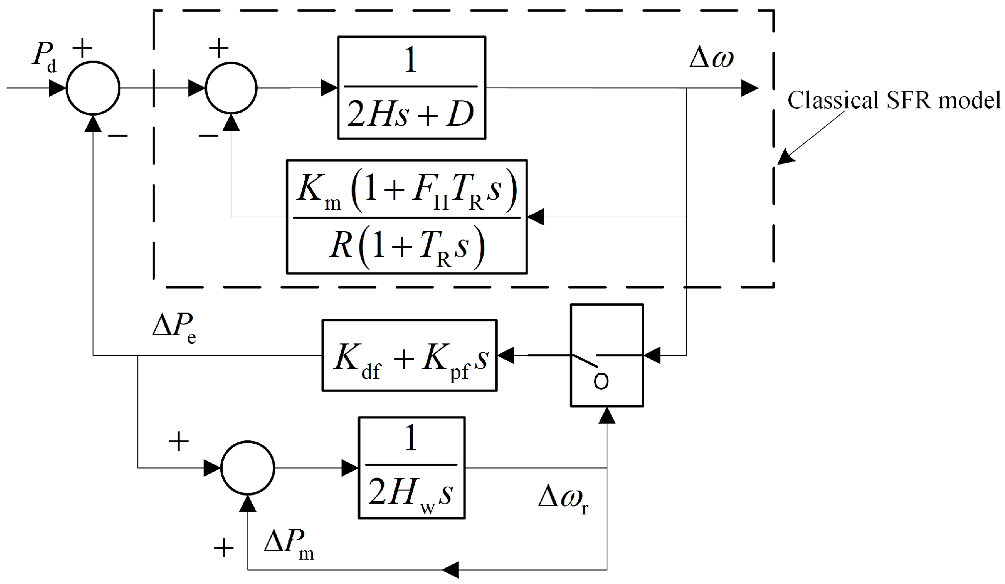
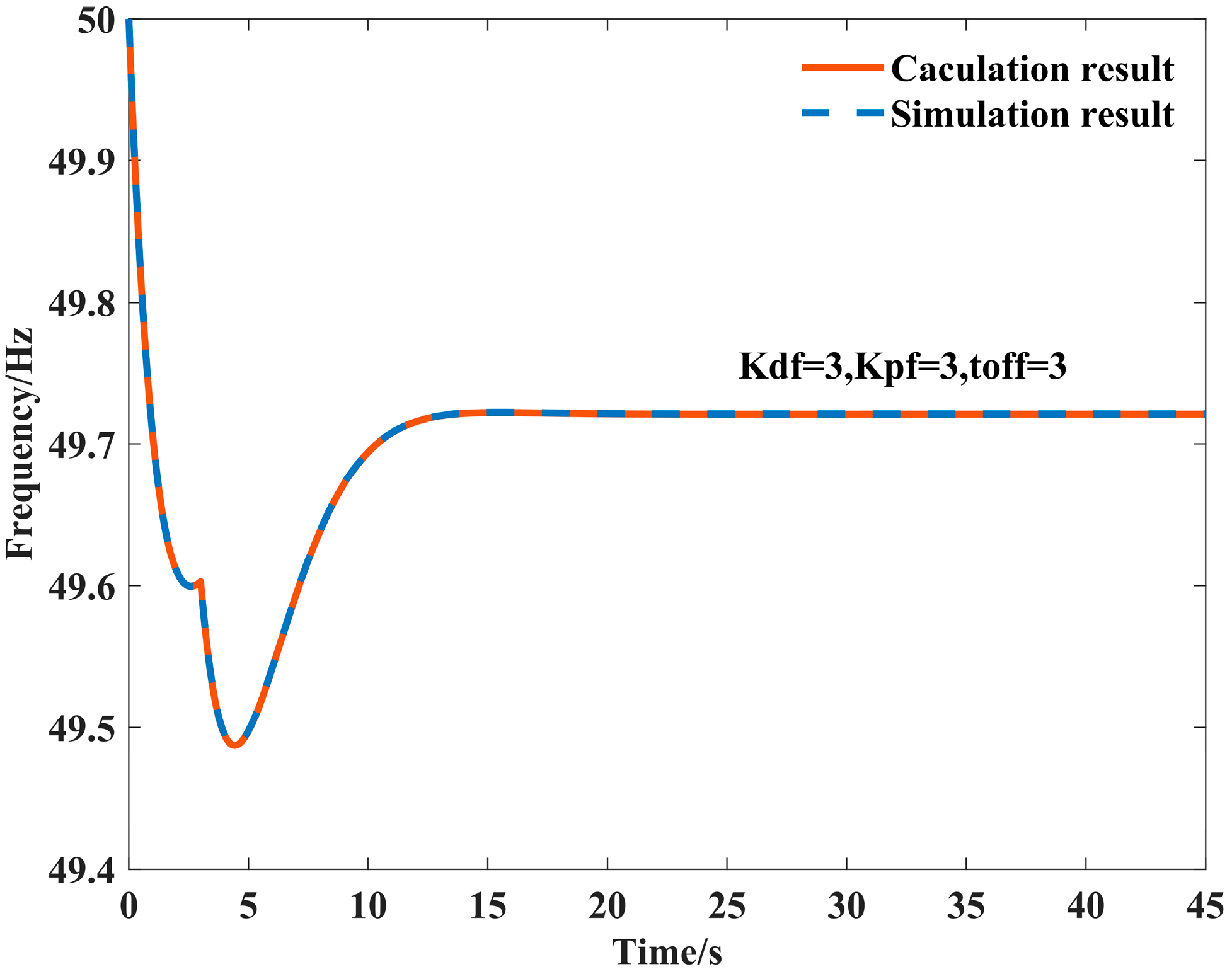
4. Dynamic Frequency Calculation Considering Wind Turbines Participating in Primary Frequency Regulation

4.1. Calculation of the Primary Frequency Drop and Its Minimum Value

When 0 < ζ< 1, the time domain expression of the system frequency variation Δf can be obtained from Equation (7) as

$$\begin{array}{ll}\Delta f(t)& =\Delta \omega (t)\\ & ={\displaystyle \frac{R{P}_{\mathrm{step}}}{DR+K_{\mathrm{m}}+R{K}_{\mathrm{df}}}}\left[1+\alpha ·\exp (-\zeta {\omega }_{\mathrm{n}}t)·\sin ({\omega }_{\mathrm{d}}t+\varphi )\right]\end{array}$$

(13)

where

$$\left\{\begin{array}{l}\alpha =\sqrt{1+{\displaystyle \frac{{(T_{\mathrm{R}}{\omega }_{\mathrm{n}}^2-\zeta {\omega }_{\mathrm{n}})}^2}{{\omega }_{\mathrm{d}}^2}}}\hfill \\ {\omega }_{\mathrm{d}}={\omega }_{\mathrm{n}}\sqrt{1-{\zeta }^2}\hfill \\ \varphi =\arctan \left({\displaystyle \frac{\sqrt{1-{\zeta }^2}}{\zeta -T_{\mathrm{R}}{\omega }_{\mathrm{n}}}}\right)\hfill \end{array}\right.$$

(14)

Equation (13) has multiple moments when the derivative is zero, as

$$t_{\mathrm{z}}={\displaystyle \frac{n\pi -{\varphi }_1}{{\omega }_{\mathrm{d}}}}$$

(15)

Substituting Equation (15) into Equation (13), the system frequency variation corresponding to these moments is

$$\Delta f_{\mathrm{ex}}(n)={\displaystyle \frac{R{P}_{\mathrm{step}}}{DR+K_{\mathrm{m}}+R{K}_{\mathrm{df}}}}\left[1+\alpha ·\exp ({\displaystyle \frac{-\zeta (n\pi -{\varphi }_1)}{\sqrt{1-{\zeta }^2}}})·\sin (n\pi -{\varphi }_2)\right]$$

(16)

where

$$\left\{\begin{array}{l}{\varphi }_2=\arctan \left({\displaystyle \frac{-\sqrt{1-{\zeta }^2}}{\zeta }}\right)\hfill \\ {\varphi }_1=\varphi +{\varphi }_2\hfill \end{array}\right.$$

(17)

It can be seen from Appendix B that when n = 1, the system frequency reaches the minimum value, and the time corresponding to the minimum value of the system frequency is

$$t_{\min }={\displaystyle \frac{(\pi -{\varphi }_1)}{{\omega }_{\mathrm{d}}}}$$

(18)

Substituting Equation (18) into Equation (16) and solving it, when 0 < ζ < 1, the minimum value of the frequency variation is

$$\Delta f_{\min }={\displaystyle \frac{R{P}_{\mathrm{step}}}{DR+K_{\mathrm{m}}+R{K}_{\mathrm{df}}}}·\left[1+\alpha ·\exp ({\displaystyle \frac{-\zeta (\pi -{\varphi }_1)}{\sqrt{1-{\zeta }^2}}})·\sin (\pi -{\varphi }_2)\right]$$

(19)

When ζ > 1, the time domain expression of Δf is

$$\begin{array}{ll}\Delta f(t)=& \Delta \omega (t)={\displaystyle \frac{R{P}_{\mathrm{step}}}{DR+K_{\mathrm{m}}+R{K}_{\mathrm{df}}}}·\left\{1-{\displaystyle \frac{1}{2\sqrt{{\zeta }^2-1}}}·\right.\\ & \left[\left({\displaystyle \frac{1}{\zeta -\sqrt{{\zeta }^2-1}}}-T_{\mathrm{R}}{\omega }_{\mathrm{n}}\right)·\exp (-(\zeta -\sqrt{{\zeta }^2-1}){\omega }_{\mathrm{n}}t)-\right.\\ & \left.\left.\left({\displaystyle \frac{1}{\zeta +\sqrt{{\zeta }^2-1}}}-T_{\mathrm{R}}{\omega }_{\mathrm{n}}\right)·\exp (-(\zeta +\sqrt{{\zeta }^2-1}){\omega }_{\mathrm{n}}t)\right]\right\}\end{array}$$

(20)

Then, the time corresponding to the minimum Δf is

$$t_{\min }={\displaystyle \frac{\ln \frac{1-T_{\mathrm{R}}{\omega }_{\mathrm{n}}\left(\zeta -\sqrt{{\zeta }^2-1}\right)}{1-T_{\mathrm{R}}{\omega }_{\mathrm{n}}\left(\zeta +\sqrt{{\zeta }^2-1}\right)}}{-2{\omega }_{\mathrm{n}}\sqrt{{\zeta }^2-1}}}$$

(21)

The lowest value of the system frequency drops when ζ > 1 is obtained from Equations (20) and (21).

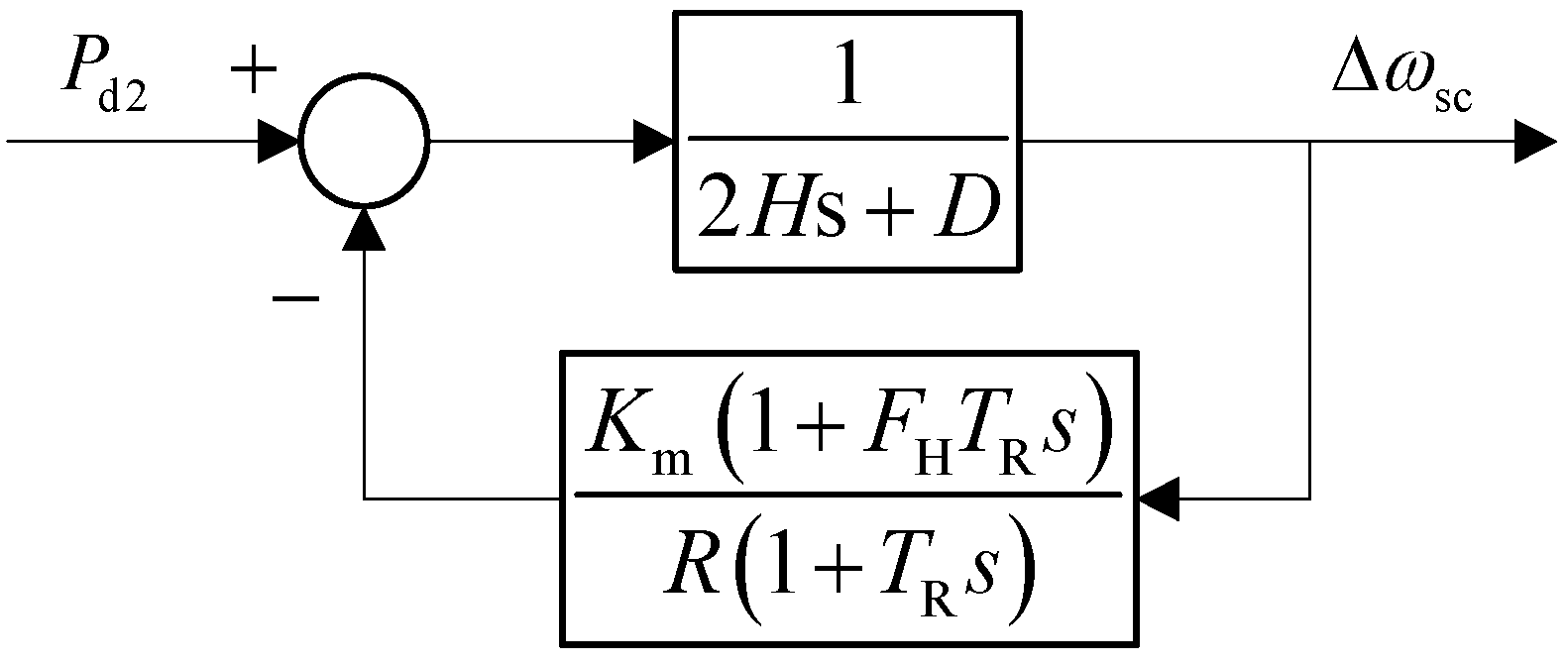
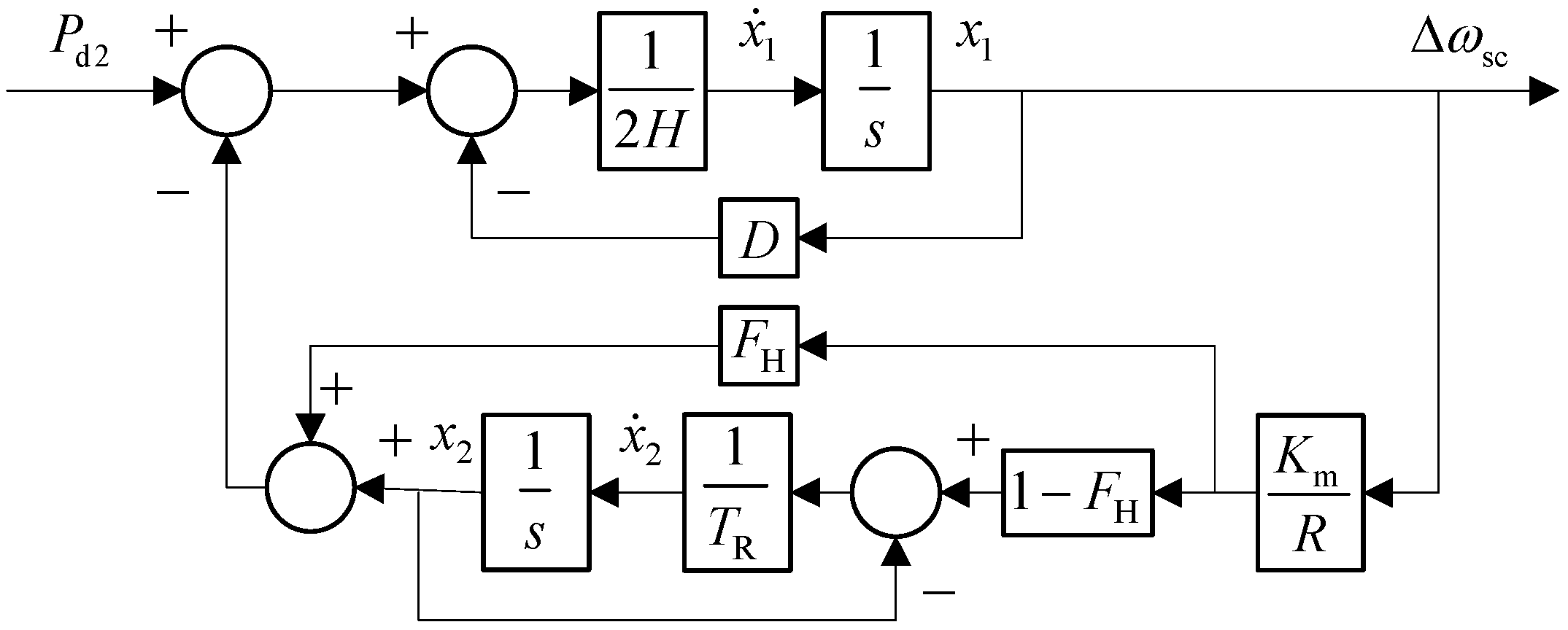
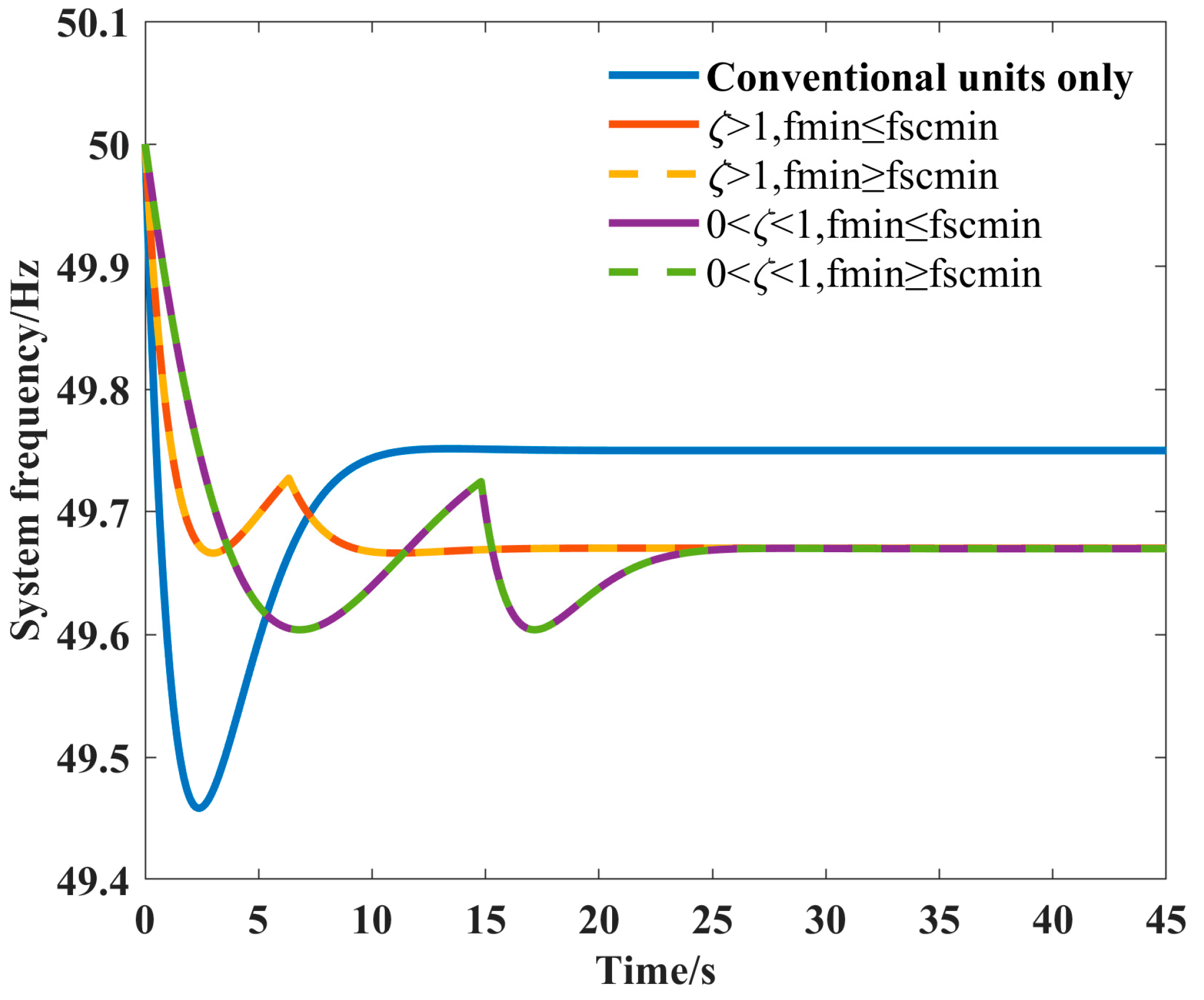
4.2. Calculation of the Secondary Frequency Drop and Its Minimum Value

When the wind turbine exits the primary frequency regulation, the switch O in Figure 2 is open and only traditional generator units in the power system continue to contribute to the primary frequency regulation. The SFR model shown in Figure 3 is established by setting the initial time t_off as the new reference point at which the wind turbine exits the primary frequency regulation. In Figure 3, P_d2 is the unbalanced power of the system at the time t_off and Δω_sc is the rotor speed variation in the traditional generator unit after the wind turbine exits primary frequency regulation.

The ratio of the wind turbine power at the MPPT point to the cube of the wind rotor speed is K_w:

$$K_{\mathrm{w}}=n_{\mathrm{w}}·{\displaystyle \frac{1}{2}}\rho \pi C_{\mathrm{pmax}}{\displaystyle \frac{R_{\mathrm{w}}^5}{{\lambda }_{\mathrm{opt}}^3}}$$

(22)

where C_pmax is the maximum wind power coefficient. λ_opt is the optimal tip speed ratio of the wind turbine.

From Equation (22), the difference ΔP_mppt between the power at the initial operating point and the power at the MPPT point of the wind turbine at the moment that the wind turbine exits the primary frequency regulation is

$$\Delta P_{\mathrm{mppt}}=K_{\mathrm{w}}[{\omega }_{\mathrm{r}0}^3-{({\omega }_{\mathrm{r}0}+\Delta {\omega }_{\mathrm{roff}})}^3]$$

(23)

where Δω_r0 is the wind turbine initial rotor speed.

P_d2 is still a step function, and the step amount is

$$P_{\mathrm{step}2}=P_{\mathrm{step}}-\Delta P_{\mathrm{mppt}}$$

(24)

Figure 1 illustrates that P_d2 should also include the power component of the wind turbine rotor speed recovery stage, but the recovery time is long, and the electromagnetic power of the wind turbine changes relatively slowly, which has limited influence on the system frequency [9]. In order to simplify the analysis, this paper ignores the influence of the wind turbine rotor speed recovery stage on the secondary frequency drop.

Decompose the SFR model in Figure 3, as shown in Figure 4. The SFR model, following decomposition, comprises two state variables, x₁ and x₂.

The expression in state space of the decomposed SFR model in Figure 4 is

$$\left\{\begin{array}{c}\dot{\mathit{x}}={\mathit{A}}_{\mathbf{sc}}\mathit{x}+{\mathit{B}}_{\mathbf{sc}}\mathit{u}\\ \mathit{y}={\mathit{C}}_{\mathbf{sc}}\mathit{x}+{\mathit{D}}_{\mathrm{sc}}\mathit{u}\end{array}\right.$$

(25)

where

$$\left\{\begin{array}{l}{\mathit{A}}_{\mathbf{sc}}=\left[\begin{array}{cc}-{\displaystyle \frac{K_{\mathrm{m}}{F}_{\mathrm{H}}+DR}{2HR}}& -{\displaystyle \frac{1}{2H}}\\ {\displaystyle \frac{K_{\mathrm{m}}(1-F_{\mathrm{H}})}{R{T}_{\mathrm{R}}}}& -{\displaystyle \frac{1}{T_{\mathrm{R}}}}\end{array}\right]\\ {\mathit{B}}_{\mathbf{sc}}=\left[\begin{array}{c}{\displaystyle \frac{1}{2H}}\\ 0\end{array}\right]\\ {\mathit{C}}_{\mathbf{sc}}=\left[\begin{array}{cc}1& 0\end{array}\right]\\ {\mathit{D}}_{\mathrm{sc}}=0\end{array}\right.$$

(26)

Assuming that the initial value of the state vector is x(0), solve Equation (25).

$$Y(s)={\mathit{C}}_{\mathbf{sc}}{(s\mathit{I}-{\mathit{A}}_{\mathbf{sc}})}^{-1}[\mathit{x}(0)+{\mathit{B}}_{\mathbf{sc}}U(s)]$$

(27)

where

$$\left\{\begin{array}{l}U(s)={\displaystyle \frac{P_{\mathrm{step}2}}{s}}\hfill \\ \mathit{x}(0)=\left[\begin{array}{c}{x}_1(0)\\ x_2(0)\end{array}\right]\hfill \end{array}\right.$$

(28)

Simplifying Equation (27), the system frequency deviation Δf_sc after the wind turbine exits primary frequency regulation is

$$\begin{array}{ll}\Delta f_{\mathrm{sc}}(s)=& \Delta {\omega }_{\mathrm{sc}}(s)={\displaystyle \frac{R{P}_{\mathrm{step}2}}{DR+K_{\mathrm{m}}}}·{\displaystyle \frac{(1+T_{\mathrm{R}}s){\omega }_{\mathrm{n}}^{\prime 2}}{s(s^2+2{\zeta }^{\prime }{\omega }_{\mathrm{n}}^{\prime }s+{\omega }_{\mathrm{n}}^{\prime 2})}}+\\ & {\displaystyle \frac{x_1(0)}{T_{\mathrm{R}}}}·{\displaystyle \frac{1+T_{\mathrm{R}}s}{s^2+2{\zeta }^{\prime }{\omega }_{\mathrm{n}}^{\prime }s+{\omega }_{\mathrm{n}}^{\prime 2}}}-\\ & {\displaystyle \frac{x_2(0)}{2H}}·{\displaystyle \frac{1}{s^2+2{\zeta }^{\prime }{\omega }_{\mathrm{n}}^{\prime }s+{\omega }_{\mathrm{n}}^{\prime 2}}}\end{array}$$

(29)

where

$$\left\{\begin{array}{l}{\omega }_{\mathrm{n}}^{\prime 2}={\displaystyle \frac{DR+K_{\mathrm{m}}}{2HR{T}_{\mathrm{R}}}}\hfill \\ {\xi }^{\prime }={\displaystyle \frac{2HR+(DR+K_{\mathrm{m}}{F}_{\mathrm{H}})T_{\mathrm{R}}}{2(DR+K_{\mathrm{m}})}}·{\omega }_{\mathrm{n}}^{\prime }\hfill \end{array}\right.$$

(30)

From Equation (29), the time domain expression of Δf_sc is

$$\Delta f_{\mathrm{sc}}(t)={\displaystyle \frac{R{P}_{\mathrm{step}2}}{DR+K_{\mathrm{m}}}}+{\mathrm{e}}^{-{\zeta }^{\prime }{\omega }_{\mathrm{n}}^{\prime }t}{\alpha }_{\mathrm{x}}\sin ({\omega }_{\mathrm{d}}^{\prime }t+{\varphi }_{\mathrm{x}})$$

(31)

where

$$\left\{\begin{array}{l}{\alpha }_{\mathrm{x}}=\sqrt{a_{\mathrm{x}}^2+b_{\mathrm{x}}^2}\hfill \\ {\varphi }_{\mathrm{x}}=\arctan ({\displaystyle \frac{b_{\mathrm{x}}}{a_{\mathrm{x}}}})\hfill \end{array}\right.$$

(32)

where

$$\left\{\begin{array}{l}{a}_{\mathrm{x}}={\displaystyle \frac{R{P}_{\mathrm{step}2}(T_{\mathrm{R}}{\omega }_{\mathrm{n}}^{\prime 2}-{\zeta }^{\prime }{\omega }_{\mathrm{n}}^{\prime })}{(DR+K_{\mathrm{m}}){\omega }_{\mathrm{d}}^{\prime }}}+\\ {\displaystyle \frac{x_1(0)(1-{\zeta }^{\prime }{\omega }_{\mathrm{n}}^{\prime }{T}_{\mathrm{R}})}{T_{\mathrm{R}}{\omega }_{\mathrm{d}}^{\prime }}}-{\displaystyle \frac{x_2(0)}{2H{\omega }_{\mathrm{d}}^{\prime }}}\\ b_{\mathrm{x}}=-{\displaystyle \frac{R{P}_{\mathrm{step}2}}{DR+K_{\mathrm{m}}}}+x_1(0)\end{array}\right.$$

(33)

Substituting the moment when the first derivative is zero into Equation (31), the minimum value of the secondary frequency drop is

$$\Delta f_{\mathrm{scmin}}={\displaystyle \frac{R{P}_{\mathrm{step}2}}{DR+K_{\mathrm{m}}}}+{\alpha }_{\mathrm{x}}·\exp ({\displaystyle \frac{-{\zeta }^{\prime }(\pi -{\varphi }_{\mathrm{x}1})}{\sqrt{1-{\zeta }^{\prime 2}}}})·\sin (\pi -{\varphi }_{\mathrm{x}2})$$

(34)

where

$$\left\{\begin{array}{l}{\varphi }_{\mathrm{x}2}=\arctan \left({\displaystyle \frac{-{\omega }_{\mathrm{d}}^{\prime }}{{\zeta }^{\prime }{\omega }_{\mathrm{n}}^{\prime }}}\right)\hfill \\ {\varphi }_{\mathrm{x}1}={\varphi }_{\mathrm{x}}+{\varphi }_{\mathrm{x}2}\hfill \\ {\omega }_{\mathrm{d}}^{\prime }={\omega }_{\mathrm{n}}^{\prime }\sqrt{1-{\zeta }^{\prime 2}}\hfill \end{array}\right.$$

(35)

4.3. State Variable Initial Values Calculation

The state variables x₁ and x₂ are the rotor speed variation Δω_sc of the traditional power unit and the output power variation ΔP_LP of the low-pressure cylinder of the traditional generator unit, respectively; the initial value is the value at the time t_off when the wind turbine exits the primary frequency regulation.

From Figure 2, Δω(s) and ΔP_LP(s) can be obtained when the wind turbine participates in the primary frequency regulation. The expression of Δω(s) has been given in Equation (7) and ΔP_LP(s) is

$$\Delta P_{\mathrm{LP}}(s)={\displaystyle \frac{P_{\mathrm{step}}{K}_{\mathrm{m}}(1-F_{\mathrm{H}})}{DR+K_{\mathrm{m}}+R{K}_{\mathrm{df}}}}·{\displaystyle \frac{{\omega }_{\mathrm{n}}^2}{s(s^2+2\zeta {\omega }_{\mathrm{n}}s+{\omega }_{\mathrm{n}}^2)}}$$

(36)

When 0 < ζ < 1, the time domain expression of Δω(t) has been given in Equation (13) and ΔP_LP(t) is

$$\begin{array}{ll}\Delta P_{\mathrm{LP}}(t)=& {\displaystyle \frac{P_{\mathrm{step}}{K}_{\mathrm{m}}(1-F_{\mathrm{H}})}{DR+K_{\mathrm{m}}+R{K}_{\mathrm{df}}}}·\\ & \left[1-{\displaystyle \frac{1}{\sqrt{1-{\zeta }^2}}}·\exp (-\zeta {\omega }_{\mathrm{n}}t)·\sin ({\omega }_{\mathrm{d}}t+{\varphi }_{\mathrm{LP}})\right]\end{array}$$

(37)

where

$${\varphi }_{\mathrm{LP}}=\arctan ({\displaystyle \frac{\sqrt{1-{\zeta }^2}}{\zeta }})$$

(38)

When ζ > 1, the time domain expression of Δω(t) has been given in Equation (20) and ΔP_LP(t) is

$$\begin{array}{ll}\Delta P_{\mathrm{LP}}(t)=& {\displaystyle \frac{P_{\mathrm{step}}{K}_{\mathrm{m}}(1-F_{\mathrm{H}})}{DR+K_{\mathrm{m}}+R{K}_{\mathrm{df}}}}·\left\{1-{\displaystyle \frac{1}{2\sqrt{{\zeta }^2-1}}}\right.·\\ & \left.\left.\left[{\displaystyle \frac{\exp (-(\zeta -\sqrt{{\zeta }^2-1}){\omega }_{\mathrm{n}}t)}{\zeta -\sqrt{{\zeta }^2-1}}}-\right.{\displaystyle \frac{\exp (-(\zeta +\sqrt{{\zeta }^2-1}){\omega }_{\mathrm{n}}t)}{\zeta +\sqrt{{\zeta }^2-1}}}\right]\right\}\end{array}$$

(39)

According to the values of ζ, the wind turbine primary frequency regulation exiting time t_off is substituted into Equation (13), Equation (37) or Equation (20), Equation (39), and the initial values of the state variables x₁(0) and x₂(0) are obtained.

5. Parameters Optimization of the Wind Turbine Participating in Primary Frequency Regulation

5.1. Optimization Objective and Solution Vector

Taking the minimum values both of the primary and secondary frequency drops when the wind turbine participates in the primary frequency regulation as the optimization objective, a set of multivariate function nonlinear optimization models is constructed.

Discussion on the classification of optimization objective function z is as follows. When the primary frequency drop is more severe, the minimum value of the primary drop should be as high as possible, otherwise the minimum value of the secondary frequency drop should be as high as possible. Therefore, the optimization objective function of the primary frequency regulation control parameters of the wind turbine is

$$\left\{\begin{array}{l}z=\max (\Delta f_{\min }),\Delta f_{\min }\le \Delta f_{\mathrm{scmin}}\hfill \\ z=\max (\Delta f_{\mathrm{scmin}}),\Delta f_{\min }\ge \Delta f_{\mathrm{scmin}}\hfill \end{array}\right.$$

(40)

The primary frequency regulation effect of the wind turbine is influenced by three factors: the droop control parameter K_df, the virtual inertia control parameter K_pf and the exiting time t_off. Therefore, the solution vector of the optimization model is

$${\mathit{x}}_{\mathbf{o}}=[K_{\mathrm{df}},K_{\mathrm{pf}},t_{\mathrm{off}}]$$

(41)

5.2. Constraint Conditions

The optimization model of wind turbine primary frequency control parameters contains several equality and inequality constraints.

When 0 < ζ < 1, simultaneous Equations (12), (18), (19) and (34), the equality constraints are

$$\left\{\begin{array}{l}\Delta {\omega }_{\mathrm{roff}}=\Delta {\omega }_{\mathrm{r}{K}_{\mathrm{df}}}(t_{\mathrm{off}})+\Delta {\omega }_{\mathrm{r}{K}_{\mathrm{pf}}}(t_{\mathrm{off}})\hfill \\ \Delta f_{\min }={\displaystyle \frac{R{P}_{\mathrm{step}}}{DR+K_{\mathrm{m}}+R{K}_{\mathrm{df}}}}·\left[1+\alpha ·\exp ({\displaystyle \frac{-\zeta (\pi -{\varphi }_1)}{\sqrt{1-{\zeta }^2}}})·\sin (\pi -{\varphi }_2)\right]\hfill \\ t_{\min }={\displaystyle \frac{(\pi -{\varphi }_1)}{{\omega }_{\mathrm{d}}}}\hfill \\ \Delta f_{\mathrm{scmin}}={\displaystyle \frac{R{P}_{\mathrm{step}2}}{DR+K_{\mathrm{m}}}}+{\alpha }_{\mathrm{x}}·\exp ({\displaystyle \frac{-{\zeta }^{\prime }(\pi -{\varphi }_{\mathrm{x}1})}{\sqrt{1-{\zeta }^{\prime 2}}}})·\sin (\pi -{\varphi }_{\mathrm{x}2})\hfill \end{array}\right.$$

(42)

When ζ > 1, simultaneous Equations (12), (20), (21) and (34), the equality constraints are

$$\left\{\begin{array}{l}\Delta {\omega }_{\mathrm{roff}}=\Delta {\omega }_{\mathrm{r}{K}_{\mathrm{df}}}(t_{\mathrm{off}})+\Delta {\omega }_{\mathrm{r}{K}_{\mathrm{pf}}}(t_{\mathrm{off}})\\ \begin{array}{ll}\Delta f(t)=& {\displaystyle \frac{R{P}_{\mathrm{step}}}{DR+K_{\mathrm{m}}+R{K}_{\mathrm{df}}}}·\left\{1-{\displaystyle \frac{1}{2\sqrt{{\zeta }^2-1}}}·\right.\\ & \left[\left({\displaystyle \frac{1}{\zeta -\sqrt{{\zeta }^2-1}}}-T_{\mathrm{R}}{\omega }_{\mathrm{n}}\right)·\exp (-(\zeta -\sqrt{{\zeta }^2-1}){\omega }_{\mathrm{n}}t)-\right.\\ & \left.\left.\left({\displaystyle \frac{1}{\zeta +\sqrt{{\zeta }^2-1}}}-T_{\mathrm{R}}{\omega }_{\mathrm{n}}\right)·\exp (-(\zeta +\sqrt{{\zeta }^2-1}){\omega }_{\mathrm{n}}t)\right]\right\}\end{array}\\ t_{\min }={\displaystyle \frac{\ln \frac{1-T_{\mathrm{R}}{\omega }_{\mathrm{n}}(\zeta -\sqrt{{\zeta }^2-1})}{1-T_{\mathrm{R}}{\omega }_{\mathrm{n}}(\zeta +\sqrt{{\zeta }^2-1})}}{-2{\omega }_{\mathrm{n}}\sqrt{{\zeta }^2-1}}}\\ \Delta f_{\mathrm{scmin}}={\displaystyle \frac{R{P}_{\mathrm{step}2}}{DR+K_{\mathrm{m}}}}+{\alpha }_{\mathrm{x}}·\exp ({\displaystyle \frac{-{\zeta }^{\prime }(\pi -{\varphi }_{\mathrm{x}1})}{\sqrt{1-{\zeta }^{\prime 2}}}})\sin (\pi -{\varphi }_{\mathrm{x}2})\end{array}\right.$$

(43)

Simultaneous Equations (20) and (21) separately lead to the equational constraints on Δf_min for ζ > 1.

In order to verify the correctness of the frequency calculation expressions more intuitively, typical parameters K_df = 3, K_pf = 3, t_off = 3 are taken and substituted into the frequency time domain expressions. Figure 5 compares the frequency curves calculated and simulated. It can be seen that the two frequency curves overlap with each other during the entire simulation time.

The inequality constraints of the optimization model are follows.

(1) In order to ensure the stable operation of the wind turbine, the rotor speed of the wind turbine cannot be lower than the operation limit value of 0.7 p.u. and the constraint is

$$-\Delta {\omega }_{\mathrm{roff}}-({\omega }_{\mathrm{r}0}-0.7)<0$$

(44)

(2) The traditional generator units should have sufficient time to the system frequency deviation, and the wind turbine should exit the primary frequency regulation after the system frequency drops to the minimum value. So, the constraint is

$$t_{\mathrm{off}}>t_{\min }$$

(45)

(3) According to whether the value of ζ is greater than 1 or not, an additional inequality constraint is set up, and one of the following formulas is selected as a constraint during optimization.

$$\left\{\begin{array}{l}0<\zeta <1\hfill \\ \zeta >1\hfill \end{array}\right.$$

(46)

With the wind turbines participating in the primary frequency regulation, the overall optimal value of the primary and secondary drop of the system frequency is taken as the optimization objective. Figure 6 shows the optimization process.

6. Case Study

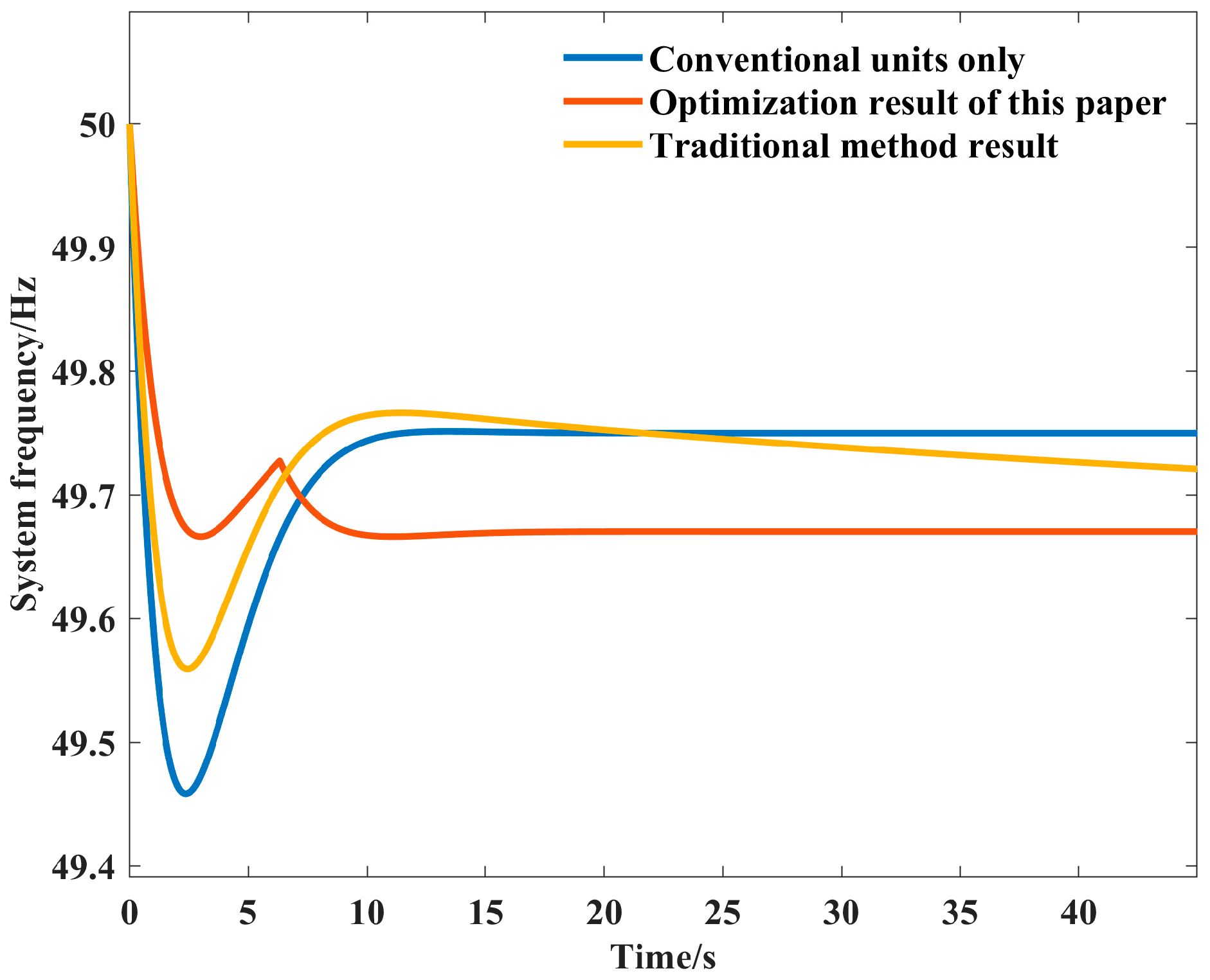
6.1. The Primary Frequency Regulation Effects of the Method Proposed in This Paper

The base value of the test system capacity is 100 MVA, the rated frequency is 50 Hz, and the output power of the conventional generator is 100 MW during normal operation. The base value of the wind turbine blade speed is 1.4273 rad/s, the wind speed is fixed at 12 m/s, the number of wind turbines participating in primary frequency regulation is 5, and the initial operating point power under the wind turbine’s single machine equivalence is 0.1185. The angular velocity ratio between the wind turbine rotor and blade is 110, the wind turbine inertia time constant is 1.0185 s, the radius of the wind turbine blade is 40 m, and the values of C₁ to C₅ are 0.22, 116, 5, 12.5, and 0, respectively. The initial rotor speed of the wind turbine is 1.3294 p.u., and the maximum wind power coefficient is 0.4328. The optimal tip speed ratio is 6.325. The air density is 1.25 kg/m³ and the value of K_cp is assumed to be 0.0602. The parameters of the conventional unit are presented in the literature [22].

The function fmincon in MATLAB version: R2020a is used to solve the optimization model. The optimization results of the wind turbine primary frequency regulation control parameters when the system disturbance power is −0.1 p.u. are presented in

Table 1. Control parameters and minimum frequency under different optimization results.

	Minimum Frequency/Hz	Droop Control Coefficient	Virtual Inertia Coefficient	Exit Time/s
When 0 < ζ < 1	49.61	0.10	28.89	14.80
When ζ > 1	49.67	5.12	6.86	6.33
Only conventional units involved	49.46	/	/	/

, and the simulation results are shown in Figure 7. As the output electromagnetic power when the wind turbine exits primary frequency regulation is less than the initial operating point power, the steady-state value of the frequency when the wind turbine participates in frequency regulation in Figure 7 will be lower than the steady-state value when only the conventional unit is used. As illustrated in Figure 7, regardless of whether ζ is greater than 1 or not, the system frequency curves obtained by solving the two optimization objectives in Equation (41), respectively, overlap completely. This indicates that the optimization process yields the optimal solution when the minimum values of the primary and second frequency drops are equal. Conversely, the system frequency dynamic curve is optimal when ζ > 1, indicating that in comparison to the control parameter of 0 < ζ < 1 when K_pf is too large and K_df is almost zero, the appropriate value of K_df has a more pronounced improvement effect on the system frequency.

Figure 8 illustrates the optimization results of the wind turbine primary frequency regulation control parameters with different disturbance powers. From Figure 8a,b, it can be observed that when the disturbance power is small, the values of K_df, K_pf, and t_off exhibit a tendency to change linearly with the disturbance power. However, they all appear to decline to varying degrees when the disturbance power exceeds −0.4 p.u.

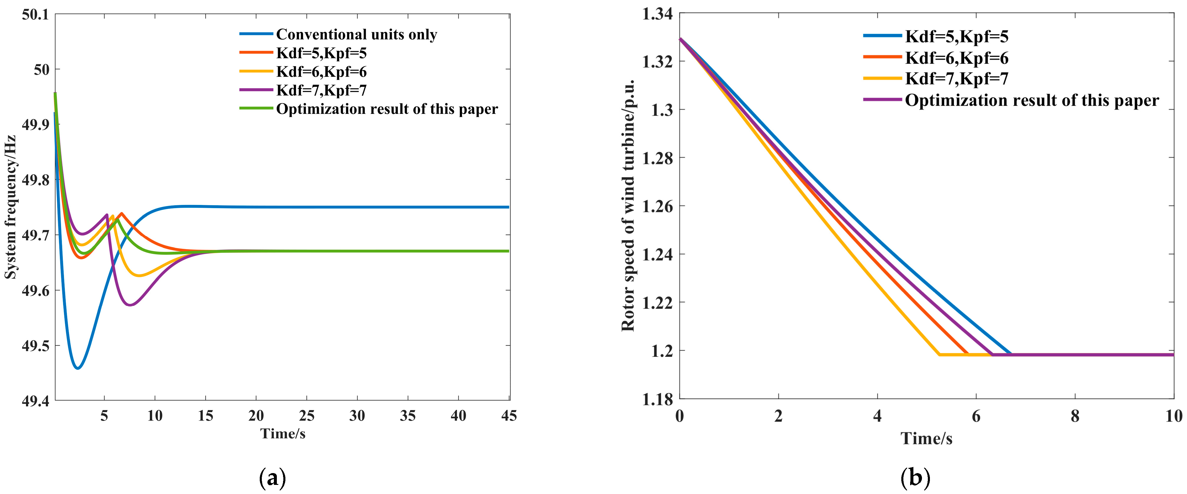
6.2. Comparison of Frequency Regulation Effects with Different Control Parameters and Strategies

The impact of the primary frequency regulation of the wind turbine on the system frequency and the wind turbine’s rotor speed is further analyzed when the control parameters take different values. Assuming that the disturbance power is −0.1 per unit, the wind turbine exits the primary frequency regulation at a fixed rotor speed, the rotor speed change is −0.1312 per unit, and the K_df and K_pf values range from 5 to 7.

Table 2. Comparison of dynamic frequency characteristics of the power system with different control parameters.

	Value of Primary Frequency Drop/Hz	Value of Secondary Frequency Drop/Hz	Exiting Time/s	Percentage of Maximum Frequency Drop
Kdf = 5, Kpf = 5	49.66	49.67	6.71	0.68%
Kdf = 6, Kpf = 6	49.68	47.63	5.84	0.74%
Kdf = 7, Kpf = 7	49.70	49.57	5.26	0.86%
Conventional units only	49.46	/	/	1.08%
The method in this paper	49.67	49.67	6.33	0.66%

shows a quantitative analysis of the percentage decline in frequency for different control parameters. The system frequency curve of primary frequency regulation of the wind turbine and the wind turbine rotor speed curve are shown in Figure 9a,b, respectively. Figure 9a illustrates that increasing K_df and K_pf can increase the minimum value of the primary frequency drop, yet simultaneously it will also have a negative impact on the minimum value of the secondary frequency drop. In addition, it can be seen from Figure 9b that there is a positive correlation between the wind turbine’s rotor speed change rate and the K_df, K_pf values. Increasing K_df and K_pf will accelerate the consumption of wind turbine’s rotor kinetic energy, resulting in an early exit time of the wind turbine primary frequency regulation.

Figure 10 compares the system frequency curves at different wind turbine primary frequency regulation exit times t_off when the disturbance power is −0.1 per unit. The figure illustrates that the minimum frequency with the wind turbine exiting at a fixed time is consistently lower than the optimal solution, regardless of whether the t_off is greater or less than the 6.33 s corresponding to the optimization strategy in this paper. This indicates that t_off should be employed as part of the parameters optimization process to match the values of K_df and K_pf to optimize the overall dynamic frequency of the system.

Figure 11 shows the comparison between the method proposed in this paper and the method of preventing the secondary frequency drop in [11]. The method proposed in this paper comprehensively considers the problem of primary and secondary frequency drops to optimize the minimum frequency of the overall process of primary frequency regulation. In contrast, the method in [11] primarily focuses on avoiding or relieving the secondary frequency drop. As illustrated in Figure 11, while the reference method effectively alleviates the issue of the secondary frequency drop, the improvement in the overall frequency minimum is limited and the optimization results are overly conservative. In contrast, although the method proposed in this paper still experiences a secondary frequency drop, the overall dynamic frequency is significantly enhanced in comparison to the traditional method, and the system is less likely to trigger the low-frequency relays. Furthermore, the method proposed in this paper shows a significant reduction in the maximum RoCoF when the frequency disturbance occurs, in addition to a delayed system frequency nadir.

7. Conclusions

This study introduces an innovative optimization approach for the control parameters of wind turbine primary frequency regulation, which significantly mitigates both primary and secondary frequency drops. Further studies could explore the scalability of this approach to larger, multi-area power systems, investigate its integration with other renewable energy sources, and develop real-time adaptive control strategies for varying power system conditions. The principal contributions and major findings of this paper are outlined as follows:

(1)

The optimization of wind turbine primary frequency regulation control parameters necessitates a precise understanding of the correlation between these parameters and the power system dynamic frequency characteristics. Furthermore, it is essential to consider the interdependent relationship between primary and secondary frequency drops within the power system. Case study analysis demonstrates that the implementation of control parameters which holistically address both primary and secondary frequency drops can substantially enhance the power system dynamic frequency performance.

(2)

The optimization results demonstrate that the power system frequency exhibits optimal dynamic characteristics when the minimum values of primary and secondary frequency drops are equivalent. This finding reveals the existence of a game-theoretic relationship between primary and secondary frequency drops.

(3)

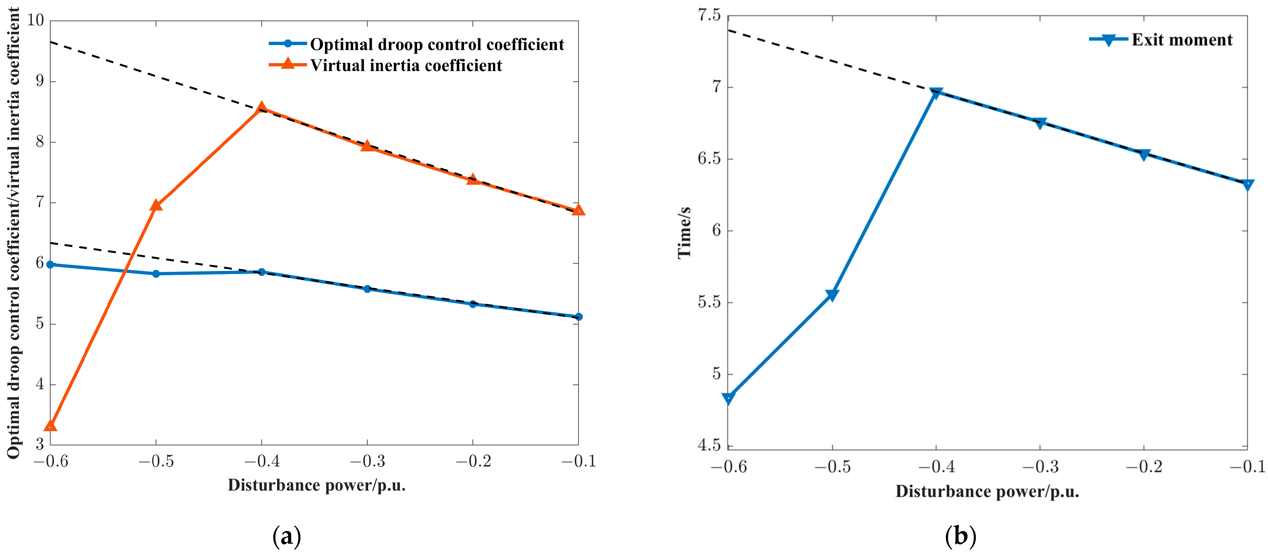
The optimal configuration of wind turbine primary frequency regulation control parameters is inherently dynamic rather than static. These parameters require coordinated tuning and real-time adjustment in response to both the magnitude of power system disturbances and the operational status of wind turbines.

References

1. Wang, R.; Qin, S.; Bao, W.; Hou, A.; Ying, Y.; Ding, L. Configuration and control strategy for an integrated system of wind turbine generator and supercapacitor to provide frequency support. Int. J. Electr. Power Energy Syst. 2023, 154, 109456. [Google Scholar] [CrossRef]
2. Messasma, C.; Barakat, A.; Chouaba, S.E.; Sari, B. PV system frequency regulation employing a new power reserve control approach and a hybrid inertial response. Electr. Power Syst. Res. 2023, 223, 109556. [Google Scholar] [CrossRef]
3. Hatziargyriou, N.; Milanovic, J.; Rahmann, C.; Ajjarapu, V.; Canizares, C.; Erlich, I.; Hill, D.; Hiskens, I.; Kamwa, I.; Pal, B.; et al. Definition and Classification of Power System Stability—Revisited & Extended. IEEE Trans. Power Syst. 2021, 36, 3271–3281. [Google Scholar]
4. Morren, J.; Haan, S.W.H.D.; Kling, W.L.; Ferreira, J.A. Wind turbines emulating inertia and supporting primary frequency control. IEEE Trans. Power Syst. 2006, 21, 433–434. [Google Scholar] [CrossRef]
5. Chen, C.; Su, Y.; Yang, T.; Huang, Z. Virtual inertia coordination control strategy of DFIG-based wind turbine for improved grid frequency response ability. Electr. Power Syst. Res. 2023, 216, 109076. [Google Scholar] [CrossRef]
6. Boyle, J.; Littler, T.; Muyeen, S.M.; Foley, A.M. An alternative frequency-droop scheme for wind turbines that provide primary frequency regulation via rotor speed control. Int. J. Electr. Power Energy Syst. 2021, 133, 107219. [Google Scholar] [CrossRef]
7. Wang, S.; Tomsovic, K. A Novel Active Power Control Framework for Wind Turbine Generators to Improve Frequency Response. IEEE Trans. Power Syst. 2018, 33, 6579–6589. [Google Scholar] [CrossRef]
8. Morren, J.; Pierik, J.; de Haan, S.W.H. Inertial response of variable speed wind turbines. Electr. Power Syst. Res. 2006, 76, 980–987. [Google Scholar] [CrossRef]
9. Bao, W.; Ding, L.; Liu, Z.; Zhu, G.; Kheshti, M.; Wu, Q.; Terzija, V. Analytically derived fixed termination time for stepwise inertial control of wind turbines—Part I: Analytical derivation. Int. J. Electr. Power Energy Syst. 2020, 121, 106120. [Google Scholar] [CrossRef]
10. Kang, M.; Muljadi, E.; Hur, K.; Kang, Y.C. Stable Adaptive Inertial Control of a Doubly-Fed Induction Generator. IEEE Trans. Smart Grid 2016, 7, 2971–2979. [Google Scholar] [CrossRef]
11. Kang, M.; Kim, K.; Muljadi, E.; Park, J.W.; Kang, Y.C. Frequency Control Support of a Doubly-Fed Induction Generator Based on the Torque Limit. IEEE Trans. Power Syst. 2016, 31, 4575–4583. [Google Scholar] [CrossRef]
12. Sun, M.; Min, Y.; Xiong, X.; Chen, L.; Zhao, L.; Feng, Y.; Wang, B. Practical Realization of Optimal Auxiliary Frequency Control Strategy of Wind Turbine Generator. J. Mod. Power Syst. Clean Energy 2022, 10, 617–626. [Google Scholar] [CrossRef]
13. Meng, L.; Qin, C.; Zeng, Y.; Sun, B.; Chen, Q.; Chen, W. A two-stage frequency response method for DFIGs under variable wind speeds. Electr. Power Syst. Res. 2023, 225, 109813. [Google Scholar] [CrossRef]
14. Wu, Y.K.; Yang, W.H.; Hu, Y.L.; Dzung, P.Q. Frequency Regulation at a Wind Farm Using Time-Varying Inertia and Droop Controls. IEEE Trans. Ind. Appl. 2019, 55, 213–224. [Google Scholar] [CrossRef]
15. Gao, H.; Zhang, F.; Ding, L.; Cornélusse, B.; Zhang, G.; Salimu, A. Multi-segment droop control and optimal parameter setting strategy of wind turbine for frequency regulation. Int. J. Electr. Power Energy Syst. 2024, 158, 109968. [Google Scholar] [CrossRef]
16. Nie, Y.; Liu, J.; Gao, L.; Wu, Y.; Li, Z. Nonlinear rotor kinetic energy control strategy of DFIG-based wind turbine participating in grid frequency regulation. Electr. Power Syst. Res. 2023, 223, 109678. [Google Scholar] [CrossRef]
17. Sun, M.; Min, Y.; Chen, L.; Hou, K.; Xia, D.; Mao, H. Optimal auxiliary frequency control of wind turbine generators and coordination with synchronous generators. CSEE J. Power Energy Syst. 2021, 7, 78–85. [Google Scholar]
18. Lin, C.H.; Wu, Y.K. Coordinated Frequency Control Strategy for VSC-HVDC-Connected Wind Farm and Battery Energy Storage System. IEEE Trans. Ind. Appl. 2023, 59, 5314–5328. [Google Scholar] [CrossRef]
19. Xiong, L.; Yang, S.; Huang, S.; He, D.; Li, P.; Khan, M.W.; Wang, J. Optimal Allocation of Energy Storage System in DFIG Wind Farms for Frequency Support Considering Wake Effect. IEEE Trans. Power Syst. 2022, 37, 2097–2112. [Google Scholar] [CrossRef]
20. Rahimi, T.; Ding, L.; Kheshti, M.; Faraji, R.; Guerrero, J.M.; Tinajero, G.D.A. Inertia Response Coordination Strategy of Wind Generators and Hybrid Energy Storage and Operation Cost-Based Multi-Objective Optimizing of Frequency Control Parameters. IEEE Access 2021, 9, 74684–74702. [Google Scholar] [CrossRef]
21. Xia, Y.; Ahmed, K.H.; Williams, B.W. Wind Turbine Power Coefficient Analysis of a New Maximum Power Point Tracking Technique. IEEE Trans. Ind. Electron. 2013, 60, 1122–1132. [Google Scholar] [CrossRef]
22. Anderson, P.M.; Mirheydar, M. A low-order system frequency response model. IEEE Trans. Power Syst. 1990, 5, 720–729. [Google Scholar] [CrossRef]
Figure 1. The relationship curves between the power and rotor speed of the wind turbine.
Energies 18 01317 g001
Figure 2. Modified SFR model with primary frequency regulation of wind turbine.
Energies 18 01317 g002
Figure 3. SFR model after wind turbines exit primary frequency regulation.
Energies 18 01317 g003
Figure 4. Decomposed SFR model.
Energies 18 01317 g004
Figure 5. Comparison of frequency curves calculated and simulated.
Energies 18 01317 g005
Figure 6. Flow chart of parameters optimization of primary frequency regulation of wind turbines.
Energies 18 01317 g006
Figure 7. System frequency curves under different optimization results.
Energies 18 01317 g007
Figure 8. Optimization results of primary frequency regulation control parameters of wind turbines with different disturbance powers. (a) Optimal droop control coefficients/virtual inertia coefficients with different disturbance powers, and (b) optimal exit moments with different disturbance powers.
Energies 18 01317 g008
Figure 9. Comparison of simulation results with different control parameters. (a) The system frequency curves with the different control parameters. (b) Rotor speed deviation curves of wind turbines with different control parameters.
Energies 18 01317 g009
Figure 10. System frequency curves with the different exit moments.
Energies 18 01317 g010
Figure 11. Comparison of optimization results between the proposed method and the method of preventing secondary frequency drop.
Energies 18 01317 g011