A Comprehensive Case Study of a Full-Size BIPV Facade

Abstract

Building-integrated photovoltaic (BIPV) systems present a promising avenue for integrating renewable energy generation into urban environments. However, they pose unique challenges, including higher planning efforts and reduced yield generation compared to conventional rooftop systems. Despite these challenges, the double use of area and the high potential in urban landscapes offer compelling advantages. Modules have become highly customizable to fit architect’s requirements in sustainable yet also aesthetic building material. This paper discusses the results of a “living laboratory” in Berlin, which is both a typical building with a ventilated curtain wall and a unique showcase for BIPV technology. Through careful analysis of various factors, including module positioning, ventilation, and shading, this study demonstrates the feasibility and practicality of BIPV integration. The “living lab” not only highlights the technical viability of BIPV systems but also underscores their potential to enhance architectural aesthetics and promote sustainability and carbon-neutrality in urban landscapes.

1. Introduction

Decarbonization of the building sector is an important waypoint on the path to reducing greenhouse gas emissions to meet the goals of the Paris Climate Agreement. In Europe, an ever-increasing amount, currently 75%, of the population already lives in cities [1]. These cities consume 60 to 80% of energy and, therefore, emit around 75% of Europe’s CO₂ emissions [2]. About 40% of these emissions result from the building sector, including the construction, renovation, and also the operation of buildings [3]. Therefore, improving the energy efficiency of buildings is an important contribution to meeting the requirements of zero-emission standards and thus a sustainable future. One approach to overcome this challenge is the expanded use of photovoltaic systems, which offer carbon-neutral and decentralized clean energy right where it is needed. However, especially in urban areas, typical rooftop systems usually compete with the use of scarce rooftop space, e.g., ventilation systems, rooftop terraces, or green roofs. Formerly unused areas in urban buildings show great potential for solar activation through building-integrated PV (BIPV) systems. A technical potential for them to cover the total electricity demand of Germany lies at 26% [4].

These BIPV systems offer architects a wide range of design opportunities to integrate renewable energy solutions seamlessly into building aesthetics. Unlike traditional solar installations, which are often perceived as bulky add-ons to buildings, building-integrated systems allow for more creative and visually appealing designs. Solar panels can be seamlessly integrated into building facades, blending with architectural elements such as windows, cladding, or shading devices [5]. This integration not only enhances the visual appeal of buildings but also creates unique opportunities for passive solar design strategies, such as daylighting and solar shading [6]. Furthermore, facade-integrated PV systems enable architects to incorporate sustainable design principles from the initial stages of building design, resulting in more energy-efficient and environmentally friendly structures.

To successfully integrate PV systems into the building envelope, the solar modules must become an integral part of a building and must fulfil other building-related functions in addition to generating electricity. These functions, e.g., as a facade element, are usually primary for the building, while power generation is secondary. This also means that completely different or at least additional requirements are placed on a BIPV module compared to a solar module in a classic installation. In addition, the different integration methods of a module in the building envelope, for example as a rear-ventilated facade element or as an in-roof variant, can have a major influence on the performance of the PV system and on the long-term visual appearance of the building. These variety of options in the design and construction process led to many unique and often hardly comparable systems. Only a few approaches were made to develop a universal applicable evaluation methodology [7].

In the last years, an ever-increasing number of test-fields popped up that investigate the functionality and efficiency of BIPV systems [8,9] or aim to simplify and standardize the construction process of BIPV systems [10]. Often, small systems with less than a handful of modules are yield-monitored regarding their type of integration and their orientation towards the sun. The literature shows [11] that a research gap still prevails when it comes to the investigation of detailed module parameters for outdoor measurements of full-size systems. Especially, module temperature and rear ventilation of the PV modules have rarely been investigated for real operating buildings. Even though full-size BIPV facade systems are not that uncommon anymore, only a few of those systems are monitored in greater detail [12,13].

This paper aims to show the current feasibility and practicality of aesthetically integrating solar energy solutions into urban environments. There is still a lack of experience and understanding of real-world projects which prevents a widespread application of BIPVs. A newly constructed laboratory building with a PV system integrated into the facade shall serve as a showcase and inspire future innovations in sustainable building design. What makes this system special is the scale of the PV facade and the approach to collect not only yield data, but also intensively monitor the module temperature and rear ventilation of the modules, alongside the usual collection of location-specific weather data. Even the influence of the air gap size resulting from different facade substructures is investigated.

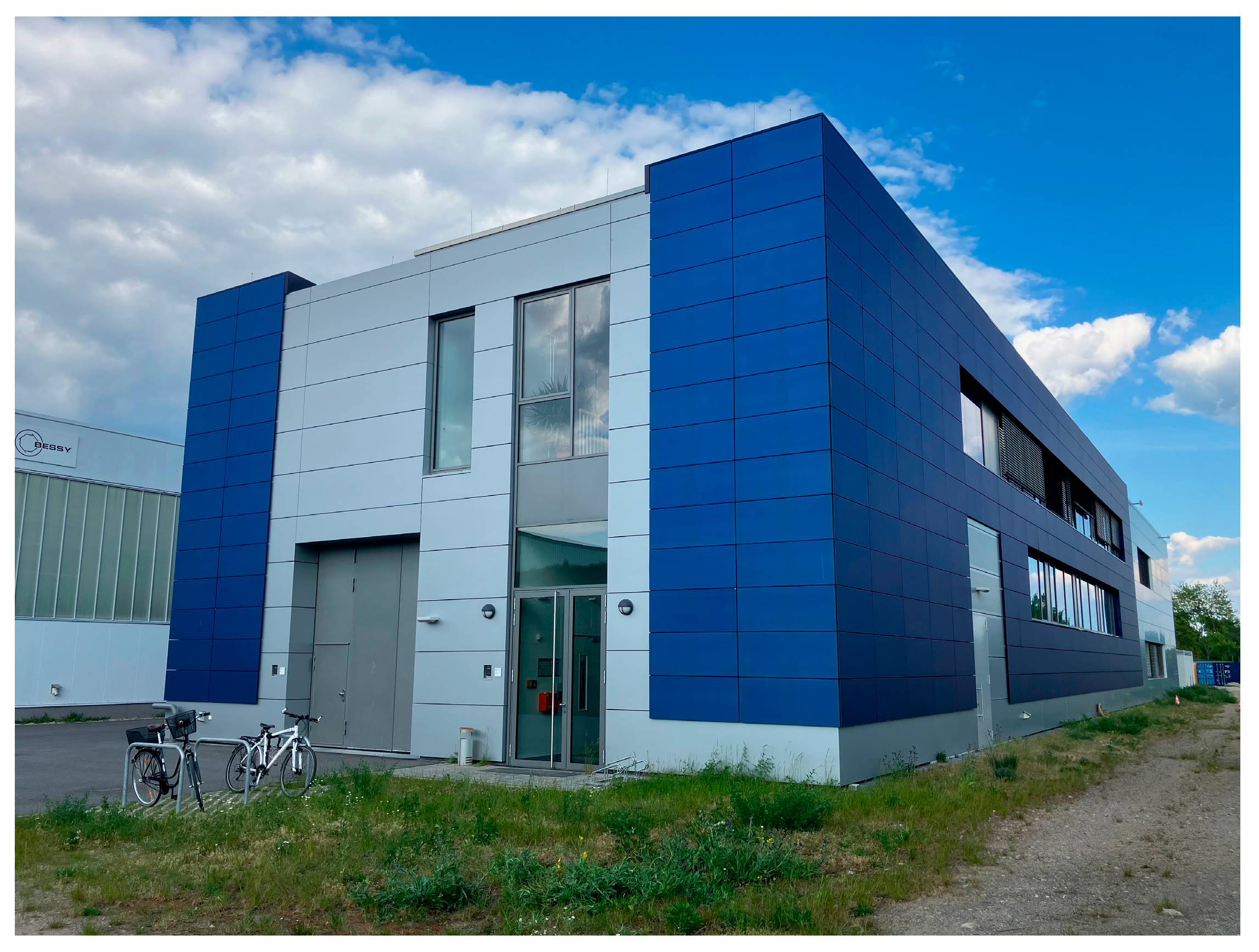
2. The Living Lab for BIPVs

Since September 2021, the Helmholtz-Zentrum Berlin (HZB) has had a new laboratory building (see Figure 1) in operation featuring an innovative integrated photovoltaic (PV) system as a ventilated curtain wall. To meticulously monitor the newly built BIPV system, a wide array of sensors was installed, augmenting the standard inverter monitoring system. This comprehensive setup includes individual string monitoring devices, temperature sensors, air flow sensors for rear ventilation measurement, pyranometers, and a complete weather station, totaling 120 sensors and measurement points. In addition to its research purposes, this laboratory building is highly frequented by both national and international visitors.

2.1. Technical Specifications

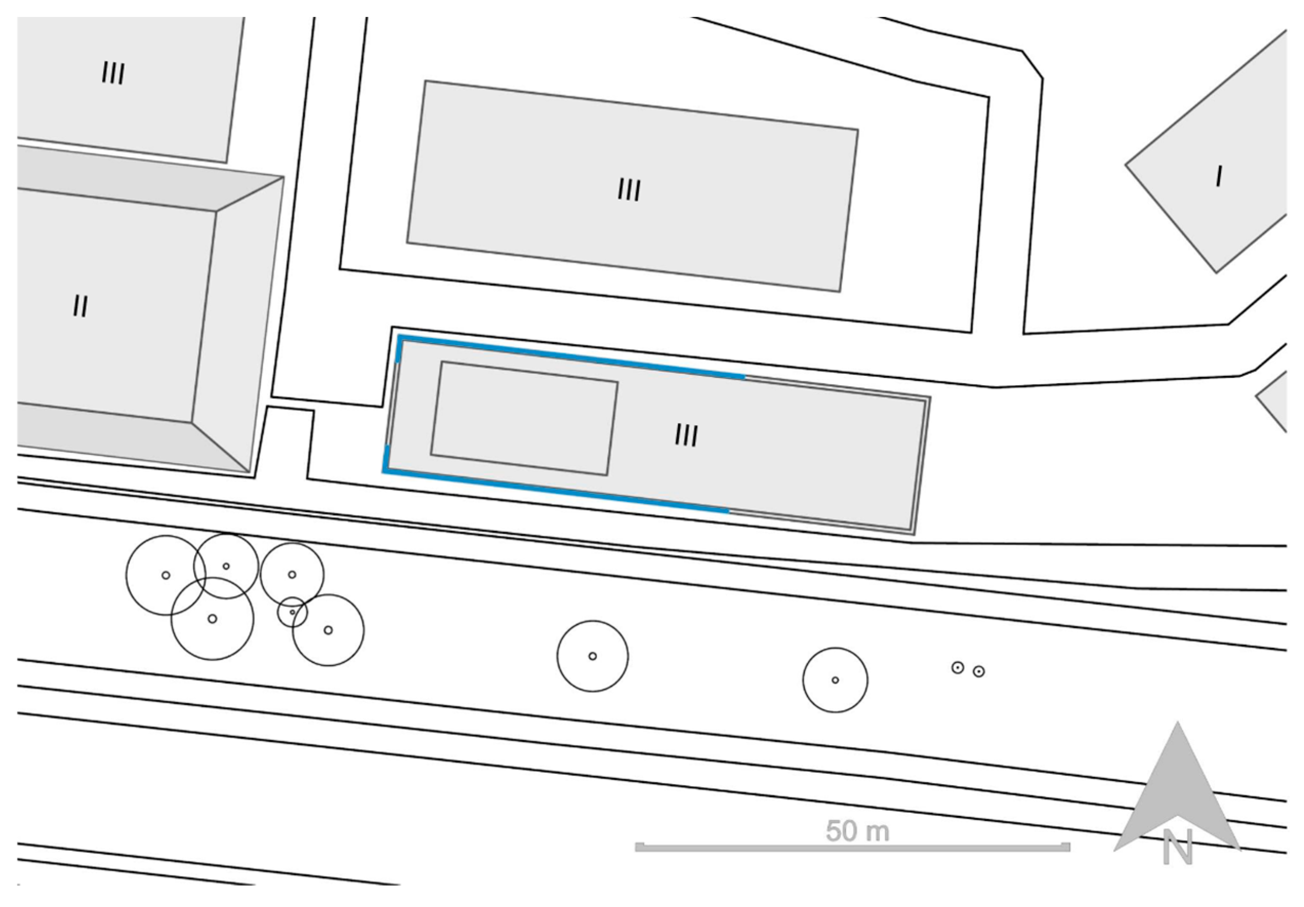
A total of 360 Copper–Indium–Gallium–Selenide (CIGS) modules were installed on three facades of the building (South, West, and North). The majority of the modules (248) are installed on the south facade, while the west facade only contains 56 modules. The north facade is equipped with the same number of modules as the west facade, even though only small yields are expected. This north facade serves as a research object in later investigations on diffuse irradiation as well as reflection and albedo measurements. The datasheet of the used modules claims that they have a nominal power of 135 Wp. The manufacturing tolerance led to minor deviations in the license plate power values ranging from 130 Wp to 142 Wp. On average, the used modules show a nominal power of 135.34 Wp. The whole system adds up to 48.72 kWp of installed power.

The PV modules were manufactured by Avancis GmbH in Torgau, Germany. The Avancis Skala 7003 modules used are frameless glass–glass modules with homogenously blue-colored front-glass. Due to the design of the modules, they appear like conventional non-solar active components. Busbars are only visible from a very close distance (<2 m). These colored modules have an efficiency of 12.3% at STC and a length-to-width ratio of 1.587 m to 0.664 m. The light-blue color is achieved by a special color technology developed by Avancis. The corresponding all-black modules (Skala B001) have an efficiency of 13.3%; thus, the relative loss in efficiency due to the colored front-glass is around 7.5% at a perpendicular incident light under STC conditions [14]. Additionally, the modules are certified as a building product by the Deutsches Institut für Bautechnik (DIBt)—the German institute for construction technologies.

To avoid power losses due to shading or generally different irradiation conditions on the different sides of the facade, the generated DC current is converted into AC current by 6 inverters, produced by the SMA Solar Technology AG in Niestetal, Germany. The modules on the north and west sides are each connected to one inverter. Four inverters are used for the significantly larger south facade. SMA specifies an efficiency of 98% for its products [15]. This 2% loss in current conversion is to be considered when comparing the measured AC current from the inverters to the measured DC current from the string monitoring devices.

For each MPP-tracker of the inverters, multiple short strings have been wired in parallel so that each can be monitored by the string monitoring devices. The layout of those strings follows two different styles on certain parts of the facade. North, west, and a small part of the south facade have been wired vertically. The most western part of the south facade is getting meticulously monitored by multiple sensors to investigate the influence of different substructure design, especially regarding the rear ventilation. A vertical string layout helps with comparing the influence of having separate strings for both substructure variations. This specific area under investigation should be comparable to other parts of the facade, which is why the exact same string layout was chosen for the two smaller facade orientations. Besides this, most of the south facade is wired horizontally, to mitigate power losses due to shading.

2.2. Location

The building is located in Berlin, Germany. In the northern hemisphere, high PV yield is usually expected in summer, with modules facing south. PV systems in Berlin achieve the overall highest annual yield at a slope angle of 40° and an azimuth angle of −4° [16]. The building under investigation is tilted slightly to the west, having the south facade at an azimuth angle of +5°.

Figure 2 shows the surrounding area of the building under investigation with the location of the nearby buildings and trees. The roman numbers on the outlined buildings indicate the height by displaying the number of floors a building has. A “III” therefore equals roughly 10 m in height, while a “II” equals roughly 7 m. South of the building, some trees grow to a height of approximately 10 m. There are some yield losses at low sun elevation, due to nearby shading objects.

3. Measurement Setup

The solar facade serves as a “living lab”. A large number of different sensors were installed. In addition to the electrical parameters, the module temperature and the rear ventilation of the modules are also to be examined. Detailed weather data are collected to validate the measured module parameters. Figure 3 shows the schematic position of every temperature (red), irradiance (yellow), and air flow sensor (green). The dark-blue area on the north facade is showing Alucobond modules, which function solely as a conventional aluminum facade cladding.

3.1. String Monitoring

Multiple strings are connected to the Maximum-Power-Point-trackers (MPP-tracker) of the inverters in parallel. Depending on the position of the string, they contain 7 to 10 modules each. As the inverters only record data per MPP-tracker, the individual strings cannot be viewed in detail. In addition to the standard string analysis by the inverters, each string is also monitored individually by additional string monitoring devices. The string monitoring devices are installed between the solar modules and the inverters in the generator connection boxes (GCBs). A total of eight ProSMS8 devices, produced by the Raycap GmbH in Garching, Germany, are installed to measure string current and voltage with an accuracy of ±1% for most of the system.

The influence of a different substructure is being investigated on the western part of the south facade. Here, another type of string monitoring device is used. A total of 3 ST2 0825 devices, produced by Kernel Sistemi in Modena, Italy, are installed. The operation of those devices differs from the Raycap devices in two points. Firstly, the Kernel devices rely on an external power source while the Raycap devices only work with sufficient power supply from the monitored strings. Secondly, the Kernel devices show a much better string current and voltage accuracy of ±0.15%. Thus, the Kernel devices provide a much more stable and precise measurement setup for this specific part of the facade.

3.2. Temperature Monitoring

Figure 3 (red dots) shows the position of the 72 temperature sensors. DS18B20 digital thermometers, produced by Maxim Integrated Products Inc. in San José, CA, USA, are glued in the center of the rear of the modules with heat-conductive adhesive. A total of 27 modules are additionally equipped with a second sensor at the edge to determine temperature differences between the edge and center.

The installed silicon bandgap temperature sensors have an operating temperature range of −55 to +125 °C. According to the data sheet, the sensors have a measuring accuracy of ±0.5% in the range from −10 to +85 °C. In Germany, this measuring range is very rarely undershot and only at night in winter [17].

3.3. Ventilation Monitoring

Figure 3 (green dots; south facade) shows the position of four air flow sensors that measure the air speed in the gap between the solar modules and the building insulation. The SCHMIDT^® Flow Sensors SS 20.500, produced by the Schmidt Technology GmbH in St. Georgen, Black Forest, Germany, are mounted on the vertical metal substructure beams in such a way that the measuring tip protrudes into the cavity behind the modules. The sensors measure with an accuracy of ±3% in a temperature range of −40 to +85 °C. The lower detection limit for wind speed is 0.06 m/s according to the data sheet.

These thermal flow sensors calculate the wind speed from an air-flow-generated temperature change. This type of sensor is suitable for measurements where the air flow may be contaminated with dirt, particles, or small insects [18]. Even though the top and bottom of the facade is protected by an insect screen, the facade is not completely sealed off. In addition, the gaps between the solar modules are big enough for insects or small particles to get into the facade.

3.4. Irradiation and Further Weather Monitoring

Figure 3 (yellow dots) shows the position of ten silicon pyranometers which are installed vertically on the three facades to record the global tilt irradiation (GTI). The coin-sized sensors (ISO 9060:2018 Class C) were glued on the inactive edge of the solar modules so that the influence on the modules due to shading is neglectable. The used ML-02 sensor, produced by EKO Instruments Co., Ltd. in Den Haag, Netherlands, has a fast response time of less than 1 ms and a sensitivity of approximately 50 µV/W/m².

In addition to the sensors at or inside the facade, a complex weather station is installed at the south-western corner on the building roof. It consists of a PVmet 500 weather station, produced by RainWise Inc. Boothwyn, PA, USA, and a sun tracker STR-21G from EKO Instruments Co., Ltd. as well as the associated shading device. The weather station acquires ambient temperature, barometric pressure, relative humidity, wind speed and direction, and the rain gauge.

Table 1. Measurement accuracy and resolution of the weather station.

Measured Parameter	Accuracy	Resolution
Ambient Temperature	±0.4 °C	0.1 °C
Barometric Pressure	±1.7 hPa	1 hPa
Relative Humidity	±5%	1%

provides the associated accuracy and resolution for these parameters except for the wind speed and direction. The accuracy and resolution of the wind measurement of the anemometer by Rainwise has not been provided. The Suntracker (ISO 9060:2018 Class A) measures GHI, diffuse global horizontal irradiance (DHI), and direct normal irradiance (DNI).

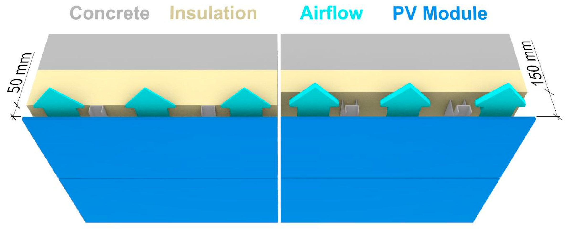
3.5. Substructure Variation

To enable the long-term study of different situations on the rear side of the modules, a selected area of the southern facade was specifically designed for the direct comparison of strings installed with different rear-side air gaps. Figure 4 schematically shows the different spacings between the PV modules and the building insulation. The major part of the building has an air gap of 150 mm defined by the necessities of architectural design with PV modules visually clamping the building. A part of the south facade was intentionally altered to a gap size of 50 mm that is closer to the conventional standard for ventilated facades without PV modules. Note that this western part of the south facade is equipped more densely with sensors (see Figure 3) to measure even small differences with higher resolution.

3.6. Data Acquisition and Measurement Gaps

In the first few years of operation, errors occasionally occurred during data acquisition. Individual sensors failed and had to be reattached or recalibrated. This led to considerable data losses in some cases. The observation period covered in this publication, from summer 2021 to summer 2023, focuses mainly on the year 2022, as this is when most of the data are available.

4. Data Analysis

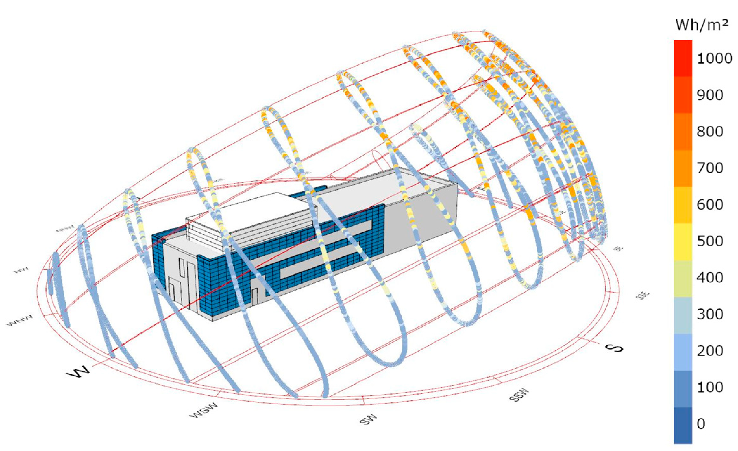
4.1. Simulation of Irradiation Conditions and PV System Performance

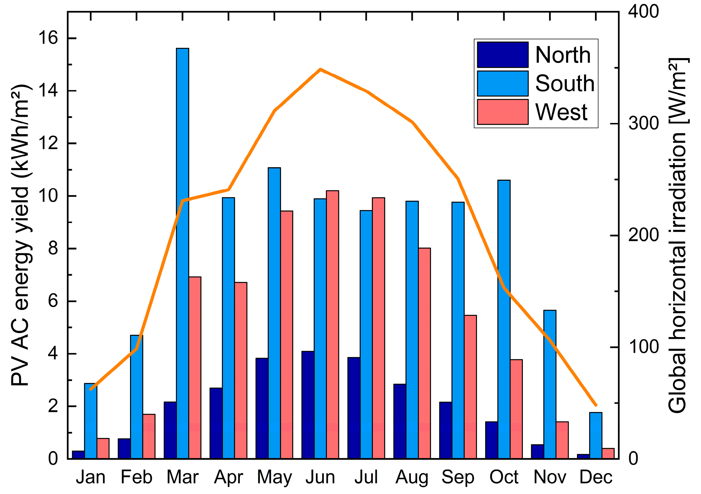
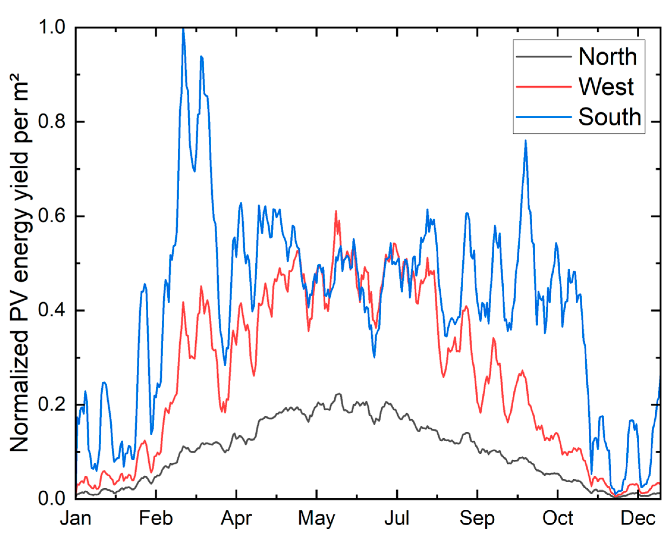
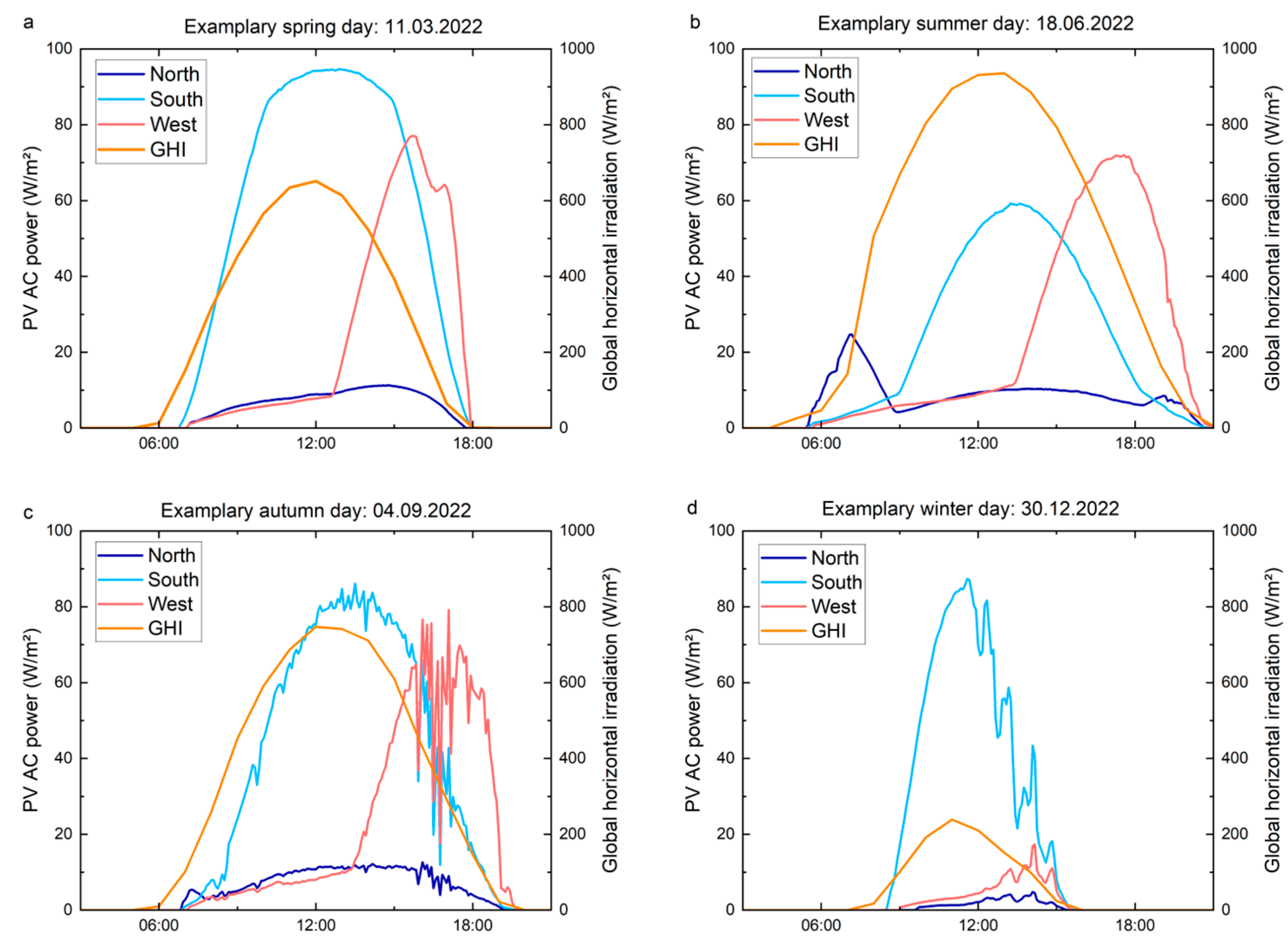
Figure 5 shows a sun path study made with the Ladybug plugin in Rhinoceros 3D (Version 7.38.24338.17001) by Robert McNeel and Associates (TLM, Inc., Seattle, WA, USA). The program simulates the sun’s motion throughout the year and color-codes it by the global horizontal irradiation (GHI). An orange dot marks high irradiation, while blue marks low irradiation. The simulation is utilizing a typical meteorological year for Berlin provided by the German meteorological service (DWD). This figure can be used to visualize the expected sun hour ratio between the seasons. Also, while focusing on the color-coded dots, the average irradiation can be estimated. Additionally, shadow-casting can be predicted in the pre-planning process. Regarding the building under investigation, three findings were made in advance and described as follows: Firstly, the highest energy yield of the complete facade is not achieved during midday in summer due to the detrimental incidence angles. Secondly, the north facade will receive direct irradiation on long summer days, especially in morning hours because of the buildings tilt. Thirdly, surrounding structures, buildings, and vegetation will most certainly cast shadows on the PV facade at different times of the day, especially in winter.

The highest sun arc shows the position of the sun and the GHI for the longest day of the year, the 21 June. The lowest arc shows the same data for the shortest day of the year, the 21 December. Each loop (Analemma) of colored dots shows the integrated irradiance of a full hour of the day. Even though the highest values can be observed in European summers of up to 900 Wh/m², the angle of incidence is far from perpendicular to the modules. To reach maximum annual energy yields for PVs, system designers conduct complex calculations to find the optimum tilt angle for the modules. For the same amount of irradiance, a PV module generates the highest power output at a perpendicular angle of incidence [19]. So, even with high irradiation and the perfect azimuth angle during noon in summer, the high sun elevation is detrimental for the modules on the south facade. The highest yield values will be observed at lower sun elevation angles for facade-integrated modules, despite lower irradiation.

Due to the orientation of the building, the north facade is facing slightly to the east, while the south facade is facing slightly to the west. Since the highest yields are expected on the large south facade, and in addition to the yields of the west facade, the overall yield profile is expected to be shifted towards the afternoon. In Figure 5 the intersection points between the highest sun arc and the cardinal points north-west and north-east show that for a limited amount of time during summer the sun is shining from the north. Therefore, direct irradiation on the north facade is to be expected only for a short time in summer. For the majority of time, the north facade will only be able to produce energy from diffuse irradiation.

This preliminary simulation of the sun path does not suffice as a basis for detailed BIPV system planning. Therefore, a more in-depth simulation was executed using PV*Sol (Version 2024R8), developed by the Valentin Software GmbH in Berlin, Germany. In PV*Sol, the user models a 3D digital twin of the building and the surrounding area. PV modules and other electrical components can be selected from a large database. What sets this software apart from other PV simulation tools is the ability to properly simulate BIPV systems. Modules can be mounted on facades or other vertical areas, and by selecting the correct mounting type, the module temperature behavior will be treated differently from a standard rooftop system. The module temperature for integrated PV systems will start with a specific offset depending on their ventilation type. This software also offers a specialized shading analysis tool to calculate shading losses, which can be used to optimize the module layout and wiring for each facade. This PV*Sol simulation was not only used in the planning process of the system, but also later in the evaluation of the measured data.

4.2. PV Power

Figure 6 shows the monthly PV energy yield per square meter module area over the course of the year 2022. The month of March was exceptionally sunny and cold and lead to the highest monthly yield for the south facade. In June and July, the west facade peaks at around 10 kWh/m² and also yields more energy than the south facade in these months. The north facade peaks in summer with values ~2/5 of that of the other sides of the building. In contrast to the west and north facade, the south facade plateaus from April to October with minor fluctuations and shows no overall peak in summer. Figure 6 also shows expected relations of the different facades between each other. Taking the south facade (100 kWh/m²) as reference, the annual yields are about two thirds and one fourth for west (65 kWh/m²) and north (25 kWh/m²) facades, respectively.

Additionally, to the measured data (red), Figure 7 shows the result of two simulations of the three-facade system as installed (grey) and a roof installation of the same capacity but with optimal inclination (40°) and azimuth angle (−4°) for Berlin (black). These simulations were conducted using PV*Sol. Note that this simulation is based on weather data of a typical meteorological year (TMY) for Berlin. This standard weather data set is commonly used in the building sector in planning and preplanning processes. A TMY does not show the actual weather data from a specific year, but rather a constructed data set to minimize the influence of yearly weather fluctuations. Therefore, deviations occur for the measured results when looking at a specific year. In general, weather fluctuations in Germany can lead to deviations in the annual yields for a PV system of up to ±10% in between two years [20].

When comparing the measured and simulated facade installation (red vs. grey), March and October stick out again. The measured yield in October even exceeds the simulated yield of the optimized roof installation (black). Values in March are also close. In 2022, the PV system generated a total of 32,000 kWh of electrical energy which surpasses the forecasted yield of around 30,400 kWh by 5.3%. For 2023, in contrast, an annual yield of around 28,000 kWh was measured, which is 7.9% lower than the simulated yield. In total, as expected, a roof installation with the optimal tilt angle for the location would be more efficient per area. The simulated annual yield of the rooftop system exceeds that of the simulated facade by 41% and 39% for the measured data. Yet, the energy gain of the rooftop system over the facade system happens mainly in summer months when there is generally excess generation by field or rooftop PVs.

Figure 8 shows the daily energy yield per square meter for each facade orientation normalized to the highest measured value. What could already be seen in Figure 7 is much clearer here. In the summer months, the west facade (red) generates the same amount and sometimes even more energy per square meter than the south facade. During spring and autumn, the South facade peaks and generates significantly more energy per m² than the west facade. This helps to smoothen the generation profile of the whole system. In winter months, contributions of the south facade are generally low. The contributions in winter from the west and north facades are negligible.

The following Figure 9 shows the AC power per m² over the time of day for each facade for four exemplary clear-sky days in each season of the year. In addition, the GHI is shown in orange (right y-axis). The chosen days are the ones with highest yield in the respective months. Autumn and winter in 2022 had no full clear-sky days in Berlin. That is why the chosen days still show some fluctuations, especially in the afternoon and evening when the weather was partly cloudy.

The generation on the south facade follows the profile of the GHI curve. During cool and sunny spring and autumn days, when the generated power is highest, the facade generates around 90 W/m². In summer and winter, the south facade only reaches one third of that, but in summer, the overall yield is higher because of significantly more hours of sunshine. The west facade’s energy generation profile is shifted to the afternoon or early evening. The generated power peaks at 80 W/m² in spring and autumn and around 70 W/m² in summer. In winter, a peak is hard to determine since no clear-sky afternoon was recorded at the given location. The north facade shows a relatively smooth generation curve of around 10 W/m² for spring, summer, and autumn. In summer, a significant power spike in the morning can be observed at the north facade.

Due to the projection area of the module surface orientation towards the sun, in summer, the peak power per m² is higher for the west facade in the afternoon at lower solar angles than for the south facade at zenith, different than what would be the case for a south-facing rooftop or field installation that is tilted. In winter, with a lower sun elevation at noon, the south facade produces more power per m² than the west facade. Due to these projection area losses at high zenith angles that raise in summer, similar power peaks can be observed throughout the year for the south facade.

The unique generation profile of the north facade in summer is a result of the high amount of sun hours of the day. Usually, the profile is driven by the diffuse light. In summer, the sun already rises early in the north-east (see Figure 5) and, therefore, leads to up to three hours of direct irradiation on the facade. The same phenomenon can be observed in the late evening, when the sun sets in the north-west, allowing some direct irradiation in the time before sunset.

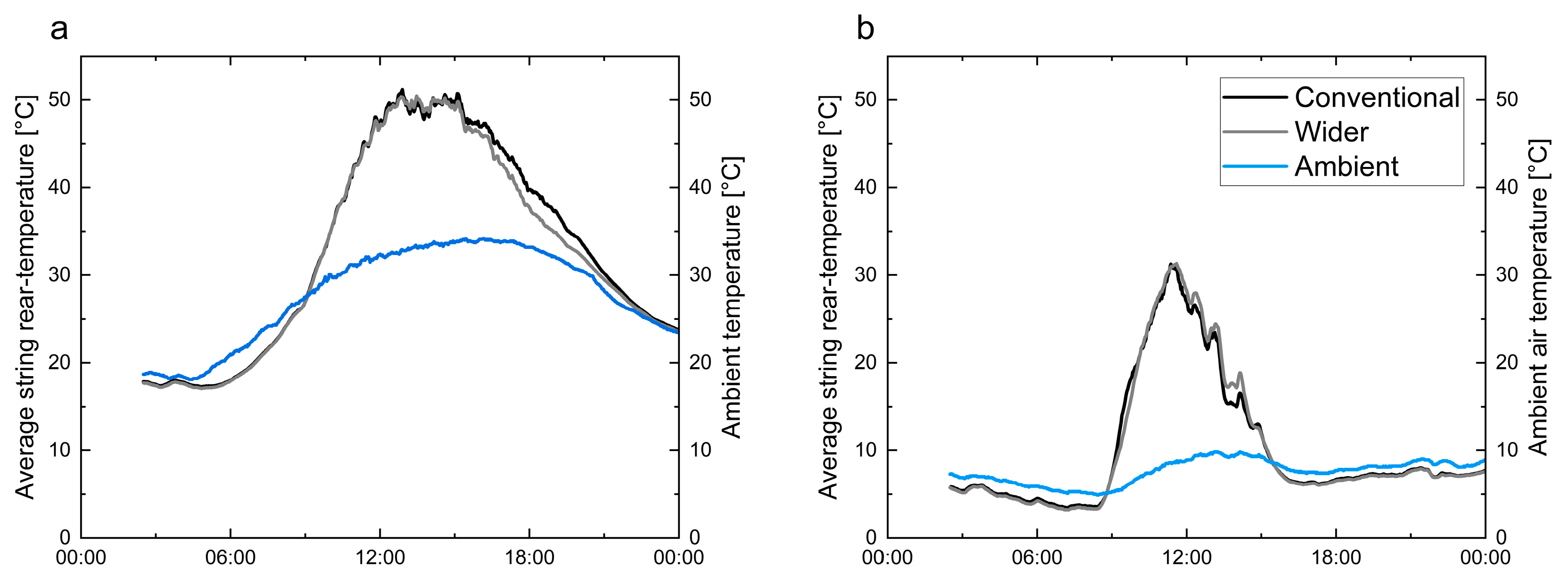
4.3. Module Temperature

Figure 10 (a) for the south, (b) west, and (c) north shows the facade temperature starting from the first measurements in July 2021 until July 2023. The measurement gaps are due to sensor failures, as described under Section 3.6. The solid line is the average value calculated from all the sensors located on the respective facade. The colored area around the average depicts the minimum and maximum of individual sensors. The temperature on the south and west facades only exceeds 60 °C in summer. The measured maximum temperature on the north facade is around 40 °C in summer. Minimum temperatures are in the single-digit negative degree range. Temperatures of −10 °C are only rarely reached on individual days in winter nights.

The temperatures on the north facade with its mainly diffuse irradiation are close to the ambient air temperature and only rarely deviate from it. On the south and west facades, the module temperature rises significantly above the ambient temperature.

In a separate module test field at HZB, the difference of a free-standing installation in comparison to the facade-integrated installation was thoroughly investigated [21]. By using the same CIGS module in the free-standing installation, only external factors resulting from the installation type influenced the module temperature. It was shown that integrated modules operate at similar temperatures in winter, while being 10 K warmer in May. The integration, therefore, only led to a relatively small power loss when taking the temperature coefficient of the module of 0.39%/°C into account.

Figure 11 shows the difference between a conventional substructure (black) and a substructure with a wider air gap (grey) regarding the average module string temperature measured on the back of the module. For comparison, the ambient air temperature is also shown (blue). The left graph (a) shows the temperature on a chosen summer day, while the right graph (b) shows it on a selected winter day. A cooling effect by the larger air gap and increased rear ventilation can hardly be observed. Only small deviations in the afternoon were measured, which are more prominent at higher temperatures in summer. Rarely, the difference is greater than 3 K, and more often, no difference is visible at all. Cooling mainly occurs via the front side through the ambient air, where the air flow is turbulent and has a much higher velocity [22].

Figure 11 shows unexpected temperature behavior at night. During nighttime, the ambient air temperature seems to be offset compared to the temperature of the facade. When further investigated, a systematic offset can be excluded, since the difference between both measurements fluctuates irregularly. A facade colder than the ambient air temperature could be explained by the thermal emissivity of the solar module and thermal radiation into space in cloudless nights.

4.4. Influence of the Rear Side Ventilation on Module Temperature and Power

The air flow velocity behind the modules depends on external weather conditions. There are openings at the top and bottom of the facade, but there are also gaps between the modules. Since the ambient wind can easily pass through those gaps, the rear ventilation speed can be very high, especially with high ambient wind speeds. This effect can be easily observed during extreme weather events like storms. Another influencing factor is the intensity of the absorbed solar irradiation. With high amounts of absorbed irradiation, the modules and the air behind them heat up. The greater the temperature difference between the ambient air and the air behind the modules, the greater the need for pressure equalization. The hot air behind the modules rises and, therefore, creates a faster air flow [23].

Figure 12a shows the air flow velocity over a day averaged, respectively, for the months from March 2022 to February 2023 for the facade area with larger spacing between the module and insulation. At night, the average air velocity is as low as 0.1 to 0.2 m/s. The average temperature profile during the day has a bell shape. Months with less irradiance peak during noon at around 0.3 to 0.5 m/s, while sunny months peak at around 0.5 to 0.7 m/s.

Figure 12b shows the same set of data for the altered substructure with the smaller air gap. With the 50 mm air gap, at night, the average air flow velocity amounts to slightly lower values of 0.05 to 0.2 m/s. At night, the air flow velocity is just a little bit slower with around 0.05 to 0.2 m/s. A significant difference can be spotted during daytime, where the air flow velocity goes from around 0.25 to 0.45 m/s. As was presented in Figure 6, March stands out with exceptionally high yield and irradiance. We also observe the highest peaks in the average air flow velocity in March. The air velocities are fortunate but not found to be exceptionally high. Temperatures are still relatively low in March 2022.

The visible difference in the average airflow velocity between the conventional air gap and the wider air gap is due to the fact that the air flow is slowed down in the area of the conventional air gap distance. Loose insulation corners and the cabling of the PV modules stand out or hang partially in the air gap. The wider air gap offers a larger space for the air to flow and, therefore, allows higher flow rates. This leads to higher heat transfer rates which cools the module faster. This positive effect is said to stagnate the wider the air gap gets, starting at about 150 mm, even when the air gap is completely free of any obstructive objects [24]. An air gap larger than that should not be any more beneficial to the module temperature and PV yield. Therefore, a standard-sized air gap in the substructure for conventional ventilated curtain-wall facades supplies sufficient ventilation for the PV modules.

5. System Cost and Amortization

As shown, standard substructure constructions are also suitable for PV facades. Nevertheless, BIPV systems usually still pose a significant increase in the investment costs of the facade. Since the modules not only entail additional costs during construction but also save electricity costs by generating energy in operation, an amortization analysis can be used as a qualitative evaluation criterion for this system. The following two questions are particularly important in this evaluation: How much higher is the initial investment? How long does it take for the additional costs to be paid off through solar activation?

The following example calculation is used to evaluate the building under investigation. The component costs depicted in

Table 2. System component cost comparison.

System Component	Cost
6× Inverters	EUR 22,800
Additional DC components	EUR 20,500
Total: PV facade (including substructure)	EUR 192,000
Total: Aluminum facade (including substructure)	EUR 65,000
Additional cost aluminum: Coloring	10.5 EUR/m2
Additional cost aluminum: Substructure fitting	16.3 EUR/m2
Additional cost aluminum: Surcharge for small-format cassettes	26.1 EUR/m2

show the actual costs (rounded) for the building under investigation. The average electricity price [25] of 0.26 EUR/kWh for non-households in Germany for the second half of 2022 was used in this calculation. Note that in the same period, the average electricity price of households in Germany is at around 0.35 EUR/kWh, thus savings would be higher if they related to residential buildings.

Total area of PV modules:

360 × 1.05 m² = 379 m²

(1)

Total area of aluminum elements:

222 × 1.05 m² = 243 m²

(2)

The costs of the PV facade, the installed inverters, and the additional DC components add to 621 EUR/m² for the entire area of the facade where PV modules were installed. An aluminum facade on this area adds up to costs of 320 EUR/m². This is 301 EUR/m² less for a non-solar active facade. Therefore, the additional costs for the PV facade in comparison to the aluminum facade are close to double the costs.

Since the HZB is a research institute with a very high energy demand of multiple Gigawatt hours per year, it operates on a dedicated campus grid to supply various research buildings. The generated PV power is always fed into this campus grid and, therefore, is always 100% self-consumed. The amount of electricity generated by the PV system must not be bought from an energy provider, charging 0.26 EUR/kWh. For the solar-active building under investigation, that means EUR 21.7 of electricity costs are saved per square meter of PV facade and year which is shown in

Table 3. Annual yield and energy saving potential per facade orientation.

Facade Orientation	Annual Yield	Annual Yield per m2	Energy Savings *
South facade	26,436 kWh/a	101.2 kWh/m2a	26.3 EUR/m2a
West facade	3821 kWh/a	64.8 kWh/m2a	16.8 EUR/m2a
North facade	1466 kWh/a	24.8 kWh/m2a	6.5 EUR/m2a
Total facade	31,723 kWh/a	83.6 kWh/m2a	21.7 EUR/m2a

* By taking 100% self-consumption into account.

. When dividing the additional costs of 301 EUR/m² for the solar activation of the facade between our annual energy savings of 21.7 EUR/m² by self-consuming the generated electricity, an amortization after 14 years can be calculated. This, however, does not take into account that inverters typically have to be changed after 10 years of operation. Including the exchange of inverters after 10 years, the amortization time for the additional costs of a BIPV facade over a standard aluminum facade increases to 17 years.

Table 4. Amortization time for different facade orientations including one exchange of inverters after 10 years.

Facade Orientation	Amortization * Time [a]
South facade	12
West facade	20
North facade	>25
Total facade	15

* Of additional costs in comparison to a standard aluminum cold facade.

shows amortization spans for the individual facade orientations of our building. Regarding the performance guarantee of the installed type of solar module, a linear degradation to 80% after 25 years was assumed. When analyzed individually, the south and west facade show amortization spans within their guaranteed lifetime of at least 25 years. As expected, the north facade will not amortize during this lifetime. Until the end of their guaranteed lifetime, the total facade system will have generated around EUR 82,000, ten years after the additional costs have been repaid.

Beyond the economic benefits of a PV system, such as the potential for energy cost savings and increased property value, it is essential to consider the broader environmental impacts. The carbon footprint reduction achieved through solar energy generation is a significant advantage that contributes to a more sustainable future. By analyzing both the economic and ecological aspects of this BIPV system, we gain a more comprehensive understanding of its overall value. Considering the German electricity mix in the national power grid, for every kilowatt hour of electricity consumed, an average of 380 g of CO₂e were emitted during generation [26]. Looking at the 30,000 kWh on average produced electricity per year, we can conclude that our living lab for BIPV saves 11.4 tons of CO₂e annually on energy not purchased, since 100% of the produced energy is self-consumed at any time of the year.

6. Conclusions

In this paper, the integrated PV facade of a laboratory building in Berlin—The Living Lab for BIPVs—was thoroughly investigated. The full-size BIPV system covers large portions of the south, west, and north facade. Several different measurement points record current data of the modules, as well as irradiance, temperature, rear-ventilation, and general weather data. The west facade contributes significantly to the overall yield. The north facade generates approximately 25% of the south facade’s annual yield, even though it lacks the number of sunshine hours. The maximum module temperature in summer is around 60 °C and, therefore, is not higher than usual roof-top installations. The influence of different air gap sizes on the rear ventilation and their effect on the module performance have also been investigated. Conventional and artificially large air gaps show no significant difference in their influence on the module performance. Besides the electrical performance of the system, it has been shown that our system is able to achieve amortization during the lifetime of the solar modules.

This innovative structure of the HZB living lab for BIPVs serves as a showcase, both for applied research and for stakeholder communication, illustrating the benefits and challenges a facade-integrated PV system entails. What sets this project apart is its role as a testing ground, where various external factors are monitored to analyze their impact on the system’s performance. Through careful analysis, the living lab demonstrates that facade-integrated PV systems are not any more technically demanding than conventional building facades or PV rooftop installations. Now that the feasibility and practicability of BIPV systems has been demonstrated, this information must be communicated primarily to architects and builders to ensure widespread use.

7. Outlook

BIPV offers a promising pathway towards carbon-neutral buildings and cities. By seamlessly integrating solar panels into a building’s architecture, BIPVs not only generates clean energy but also reduces the overall carbon footprint of the structure. Facades of urban buildings are often significantly larger than roof surfaces and can thus capture more solar energy. By using facades as energy generators, an important contribution can be made to the energy transition in cities without sacrificing valuable living space or much needed green areas. Therefore, BIPVs play a crucial role in creating sustainable and environmentally friendly communities.

Data acquired at this living lab will in the future be labelled and used for the validation of models including forecast and AI-based predictive maintenance algorithms. The closely monitored system also enables detailed studies on the influence of shading on module degradation as well as the influence of module soiling on the yield. Diffuse irradiation and albedo measurements will be closely monitored at the north facade, which will be the subject of further investigations. Installations on a north-orientated facade still may pay off, assuming long lifetimes of cheap modules, and generation times might make them interesting under current circumstances. Through further sustainable development of our research campus, more buildings will be enhanced or freshly planned with BIPV systems. We will continuously expand our range of different BIPV living labs and thus provide even deeper insights and knowledge on BIPV topics for research, application, and demonstration purposes. More living labs, case studies, and demonstrators will further help to close the gap between PV technologies and the built environment.

References

1. Department of Economic and Social Affairs. World Urbanization Prospects: The 2018 Revision; United Nations: New York, NY, USA, 2019; Available online: https://population.un.org/wup/publications/ (accessed on 3 February 2025).
2. United Nations. United Nations—Sustainable Development Goals. Available online: https://www.un.org/sustainabledevelopment/ (accessed on 3 February 2025).
3. Commission, E. Making Our Homes and Buildings Fit for a Greener Future. 2021. Available online: https://ec.europa.eu/commission/presscorner/detail/%5Beuropa_tokens:europa_interface_language%5D/fs_21_3673 (accessed on 3 February 2025).
4. Institute, B. Update on BIPV Market and Stakeholder Analysis, BIPV Boost. 2019. Available online: https://bipvboost.eu/public-reports/download/update-on-bipv-market-and-stakeholder-analysis (accessed on 3 February 2025).
5. Basher, M.K.; Nur-E-Alam, M.; Rahman, M.M.; Hinckley, S.; Alameh, K. Design, Development, and Characterization of Highly Efficient Colored Photovoltaic Module for Buildings Applications. Sustainability 2022, 14, 4278. [Google Scholar] [CrossRef]
6. Sadatifar, S.; Johlin, E. Multi-objective optimization of building integrated photovoltaic solar shades. Sol. Energy 2022, 242, 191–200. [Google Scholar] [CrossRef]
7. Wilson, H.R.; Frontini, F.; Bonomo, P.; Eder, G.C.; Babin, M.; Thorsteinsson, S.; Adami, J.; Maturi, L.; Yang, R.J.; Weerasinghe, N.; et al. Multi-dimensional evaluation of BIPV installations: Development of a tool to assess the performance as building component and electricity generator. Energy Build. 2024, 312, 114207. [Google Scholar] [CrossRef]
8. Tripathy, M.; Sadhu, P.K.; Panda, S.K. A critical review on building integrated photovoltaic products and their applications. Renew. Sustain. Energy Rev. 2016, 61, 451–465. [Google Scholar] [CrossRef]
9. Biyik, E.; Araz, M.; Hepbasli, A.; Shahrestani, M.; Yao, R.; Shao, L.; Essah, E.; Oliveira, A.C.; del Caño, T.; Rico, E.; et al. A key review of building integrated photovoltaic (BIPV) systems. Eng. Sci. Technol. Int. J. 2017, 20, 833–858. [Google Scholar] [CrossRef]
10. Chen, T.; Heng, C.K.; Leow, S. Reimagining Building Facades: The Prefabricated Unitized BIPV Walls (PUBW) for High-Rises. In Facade Design—Challenges and Future Perspektives; InTech Open: Rijeka, Croatia, 2023; pp. 1–12. [Google Scholar] [CrossRef]
11. Pillai, D.S.; Shabunko, V.; Krishna, A. A comprehensive review on building integrated photovoltaic systems: Emphasis to technological advancements, outdoor testing, and predictive maintenance. Renew. Sustain. Energy Rev. 2022, 156, 111946. [Google Scholar] [CrossRef]
12. Brozovsky, J.; Nocente, A.; Rüther, P. Modelling and validation of hygrothermal conditions in the air gap behind wood cladding and BIPV in the building envelope. Build. Environ. 2023, 228, 109917. [Google Scholar] [CrossRef]
13. Geyer, D.; Stellbogen, D.; Lechner, P.; Hummel, S.; Schnepf, J.; Huschenhöfer, D. Analysis and Investigation of BIPV Operating Performance based on the PV Installations at the ZSW Research Building. In Proceedings of the 36th European Photovoltaic Solar Energy Conference and Exhibition, Marseille, France, 9–13 September 2019; pp. 1–5. [Google Scholar] [CrossRef]
14. AVANCIS GmbH. SKALA–For Solar Facades. 2019. Available online: https://www.avancis.de/en/downloads (accessed on 3 February 2025).
15. SMA Solar Technology AG. Sunny Tripower 3.0/4.0/5.0/6.0 mit SMA SMART CONNECTED. February 2020. Available online: https://www.sma.de/en/service/downloads (accessed on 3 February 2025).
16. European Union. Photovoltaic Geographical Information System (PVGIS). European Commission. 2022. Available online: https://re.jrc.ec.europa.eu/pvg_tools/en/ (accessed on 3 February 2025).
17. Krähenmann, S.; Bissolli, P.; Rapp, J.; Ahrens, B. Spatial gridding of daily maximum and minimum temperatures in Europe. Meteorol. Atmos. Phys. 2011, 114, 3–9. [Google Scholar] [CrossRef]
18. Cerimovic, S.; Treytl, A.; Glatzl, T.; Beigelbeck, R.; Keplinger, F.; Sauter, T. Developement and Characterization of Thermal Flow Sensors for Non-Invasive Measurements in HVAC Systems. Sensors 2019, 19, 1397. [Google Scholar] [CrossRef] [PubMed]
19. Siraki, A.G.; Pillay, P. Study of optimum tilt angles for solar panels in different latitudes for urban applications. Sol. Energy 2012, 86, 1–9. [Google Scholar] [CrossRef]
20. Heesen, H.T.; Herbort, V.; Rumpler, M. Performance of roof-top PV systems in Germany from 2012 to 2018. Sol. Energy 2019, 184, 5–6. [Google Scholar] [CrossRef]
21. Ulbrich, C.; Albinius, N.; Wernke, L.; Rau, B.; Schlatmann, R. Outdoor exposure study on the performance of nine different types of industrial PV modules under 35° and under 90° tilt. In Proceedings of the 41st European Photovoltaic Solar Energy Conference and Exhibition, Vienna, Austria, 23–27 September 2024. [Google Scholar] [CrossRef]
22. Gökmen, N.; Hu, W.; Hou, P.; Chen, Z.; Sera, D.; Spataru, S. Investigation on wind speed cooling effect on PV panels in windy locations. Renew. Energy 2016, 90, 5–7. [Google Scholar] [CrossRef]
23. Ciampi, M.; Leccese, F.; Tuoni, G. Ventilated facades energy performance in summer cooling of buildings. Sol. Energy 2003, 75, 1–5. [Google Scholar] [CrossRef]
24. Gan, G. Effect of air gap on the performance of building-integrated photovoltaics. Energy 2009, 34, 913–921. [Google Scholar] [CrossRef]
25. Bundesamt, S. Database of the Federal Statistical Office of Germany. 13 June 2024. Available online: https://www-genesis.destatis.de/genesis/online?operation=sprachwechsel&language=en (accessed on 3 February 2025).
26. Icha, P.; Lauf, T. Entwicklung der Spezifischen Kohlendioxid—Emissionen des Deutschen Strommix in den Jahren 1990–2022. Umweltbundesamt, Climate Change|23/2024. 2024. Available online: https://www.umweltbundesamt.de/sites/default/files/medien/11850/publikationen/23_2024_cc_strommix_11_2024.pdf (accessed on 3 February 2025).
Figure 1. South-west view of the laboratory building with a blue PV facade, Berlin, Germany.
Energies 18 01293 g001
Figure 2. Schematic site plan of the building under investigation (plan is north orientated). The roman numbering shows the number of storys to estimate the buildings height.
Energies 18 01293 g002
Figure 3. Schematic overview of sensor placement. Temperature sensors (red), pyranometers (yellow), and air flow sensors (green). The weather station is located on the south-west corner on the roof.
Energies 18 01293 g003
Figure 4. Substructure variation with conventional substructure (left) and wider air gap (right).
Energies 18 01293 g004
Figure 5. Sun path analysis, color-coded by GHI.
Energies 18 01293 g005
Figure 6. Total PV energy yield (AC) per square meter in 2022 for the south (light blue), west (red), and north (blue) facade (GHI in orange for reference, right axes).
Energies 18 01293 g006
Figure 7. Total PV energy yield (AC) per square meter of the entire system. Comparison of real measured data (red) to a simulation of the facade (grey) to a simulation of an optimal aligned roof installation (black). (GHI in orange for reference, right axis).
Energies 18 01293 g007
Figure 8. Normalized daily energy yield per facade (normalized to south facade).
Energies 18 01293 g008
Figure 9. Facade-specific PV power per m2 (AC) for an exemplary (a) spring, (b) summer, (c) autumn, and (d) winter day. GHI for reference (orange) on secondary y-axis.
Energies 18 01293 g009
Figure 10. Minimum and maximum daily temperatures from individual sensors (area) and average facade temperature (solid line) over the course of two years as measured on the (a) south, (b) west, and (c) north facade. Missing data due to sensor failures.
Energies 18 01293 g010
Figure 11. Difference in the average module string temperature between conventional substructure (black) and substructure with wider air gap (grey) on a summer (a) and winter (b) day.
Energies 18 01293 g011
Figure 12. Average air velocity for an average day of a month. Module area with wide air gap (about 150 mm) (a) and with conventional air gap (about 50 mm) (b).
Energies 18 01293 g012