Numerical Simulation of Convective Heat Transfer in Gyroid, Diamond, and Primitive Microstructures Using Water as the Working Fluid

Abstract

With the continuous increase in the thermal power of electronic devices, air cooling is becoming increasingly challenging in terms of meeting heat dissipation requirements. Liquid cooling media have a higher specific heat capacity and better heat dissipation effect, making it a more efficient cooling method. In order to improve the heat dissipation effect of liquid cooling, a TPMS structure with a larger specific surface area, which implicit function parameters can control, can be arranged in a shape manner and it is easy to expand the structural design. It has excellent potential for application in the field of heat dissipation. At present, research is still in its initial stage and lacks comparative studies on liquid cooled convective heat transfer of TPMS structures G (Gyroid), D (Diamond), and P (Primitive). This paper investigates the heat transfer performance and pressure drop characteristics of a sheet-like microstructure composed of classic TPMS structures, G (Gyroid), D (Diamond), and P (Primitive), with a single crystal cell length of 2π (mm), a cell number of 1 × 1 × 5, and a microstructure size of 2π (mm) × 2π (mm) × 22π (mm) using a constant temperature surface model. By analyzing the outlet temperature $t_{out}$, structural pressure $p$, average convective heat transfer coefficient $h_0$, Nusselt number $Nu$, and average wall friction factor $f$ of the microstructure within the speed range of 0.01–0.11 m/s and constant temperature surface temperature is 100 °C, the heat transfer capacity D > G > P and pressure drop D > G > P were obtained (the difference in pressure drop between G and P is very small, less than 20 Pa, which can be considered consistent). When flow velocity is 0.01 m/s, the maximum temperature difference at the outlet of the four structures reached 17.14 °C, and the maximum difference in wall friction factor $f$ reached 103.264, with a relative change of 646%. When flow velocity is 0.11 m/s, the maximum pressure difference among the four structures reached 8461.84 Pa, and the maximum difference in $h_0$ reached 7513 W/(m²·K), with a relative change of 63.36%; the maximum difference between Nu reached 76.32, with a relative change of 62.09%. This paper explains the reasons for the above conclusions by analyzing the proportion of solid area on the constant temperature surface of the structure, the porosity of the structure, and the characteristics of streamlines in the microstructure.

1. Introduction

Compared with air-cooled systems, the heat transfer coefficient and specific heat capacity of the cooling working fluid in liquid cooling systems are higher than in air, resulting in higher heat transfer efficiency and better cooling effects. Compared with phase change cooling systems, the cooling fluid in liquid cooling systems has a higher thermal conductivity and better stability. Liquid cooling systems have attracted widespread attention from the industry and scholars due to their strong heat transfer performance, high integration, and low noise during operation [1]. Detailed explanations of the advantages of liquid cooling heat dissipation are provided in the papers [2,3]. This paper studies liquid cooling heat dissipation. In specific application fields, taking LED liquid cooling heat dissipation as an example, Mohamed Bechir Ben Hamida has done a series of studies, such as nanofluid filling, fin position optimization, and bubble mode absorption, and MHD, light-emitting diode arrays, and Multiwalled Carbon Nanotubes have demonstrated the advantages of liquid cooling in the field of LED heat dissipation [4,5,6,7,8,9].

TPMS is widely present in nature and can be found in similar forms in various biological structures, such as cell membranes, butterfly scales, beetle elytra, corals, and sponges [10]. The TPMS structure has attracted attention from multiple disciplines, such as mechanics, materials, chemistry, and biology, due to its excellent controllability [11]. Ref. [10] provides an overview of the structural design, manufacturing, and applications of TPMS in multiple fields. Meanwhile, TPMS provides concise and accurate descriptions for various physical structures such as silicates, dual continuous composite materials, soluble colloids, and detergent films [12]. Ref. [13] introduces the many thermal applications of TPMS, including PCM, and various fields such as adsorption desorption/cleaning, electronic thermal management, etc.

As a new type of heat dissipation structure, TPMS provides new ideas for heat dissipation design with its unique periodic pore structure and excellent fluid dynamics characteristics [14].

Traditional designs limit radiator heat exchange features’ number, size, and configuration. Compared to traditional designs and other honeycomb structures, TPMS porous structures have advantages such as larger specific surface area, more tortuous flow [15], and the ability to be controlled by mathematical equations [16]. TPMS can achieve good heat exchange and fluid pathways through parameter structure design, improving the efficiency of heat exchange systems and thus finding structures with good heat dissipation performance. However, there is still a significant gap in the current research on TPMS heat dissipation.

TPMS heat transfer research has just emerged in recent years. In 2021, ref. [17] analyzed the morphology, heat transfer, and flow characteristics of TPMS structures constructed through pore parameters for transporting gaseous CO₂. Compared with metal sintered porous media structures, TPMS structures exhibited better performance in terms of flow resistance, heat transfer coefficient, and structural strength. In 2023, ref. [18] simulated and analyzed the flow and heat transfer characteristics of several TPMS, including I-WP, Neovius, Fischer Koch S, and P, using helium as the working fluid at different Reynolds numbers. In 2023, ref. [19] studied the heat transfer characteristics of three TPMS structures, G, D2, and I-WP, with air as the working fluid and Reynolds numbers in the range of 166–940 through a combination of numerical simulation and experiments, and introduced traditional fin structures as reference objects. In 2024, ref. [20] proposed a new method of introducing a fin structure into the TPMS and named it Fin Structure TPMS (TFS). Numerical simulation was conducted on the TFS-Gyroid air-cooled radiator, and the influence of fin height on the heat transfer performance and thermal resistance of the TFS-Gyroid was studied, optimizing the structure. Refs. [21,22] are two review articles on the heat transfer of TPMS, in which the study of radiators mainly focuses on gas, and there is very little research on liquid cooling heat dissipation except for some heat exchangers that use fluids. There is also a lack of comparison and mechanism analysis between the most typical TPMS structures in the study of liquid as the working fluid. This is the starting point of this study.

The typical structures of TPMS include G (Gyroid), D (Diamond), P (Primitive), I-WP, F-RD, etc., [17,23]. Because I-WP, F-RD, and other structures are gradually constructed to solve specific mechanical problems, the basic structure adopted in the article is the most primitive G, D, and P structure.

Due to the complex internal structure of TPMS, it is necessary to study the heat transfer mechanism of micro-TPMS and determine the microstructure’s heat transfer capacity and pressure drop performance. At the same time, due to the limitations of experimental conditions, it is difficult to observe the flow and temperature distribution inside the TPMS, so its internal mechanism can be studied through numerical simulation [19,23].

This paper mainly introduces the numerical simulation of fluid heat transfer in the TPMS microstructure. All numerical simulation work was completed on the COMSOL MULTIPHYSICS 6.2 computing platform.

2. Function Representation of TPMS

TPMS stands for Three Period Minimum Surface, a type of surface with a special status in mathematics. The characteristic of these surfaces is that their average curvature $H={\displaystyle \frac{k_1+k_2}{2}}$ is zero, which means they are locally minimized in area [24,25]. The mathematical expression of the TPMS structure has various forms, and common expressions are usually parametric equations or implicit functions. The first method, Enneper Weierstrass parameterization, is a method that can accurately describe the structure of the TPMS, and its expression is as follows [26,27]:

$$x=Re{\int }_{w_0}^w{e}^{i\theta }\left(1-{\tau }^2\right)R\left(\tau \right)d\tau$$

(1)

$$y=Re{\int }_{w_0}^w{e}^{i\theta }\left(1+{\tau }^2\right)R\left(\tau \right)d\tau$$

(2)

$$z=Re{\int }_{w_0}^w{e}^{i\theta }2\tau R\left(\tau \right)d\tau$$

(3)

Among them, $Re$ is the real part, $i$ is the imaginary unit, $\theta$ is the Bonnet angle, and the surface associated with the Weierstrass function $R\left(\tau \right)$ can be guaranteed to be extremely small.

The specific form of $R\left(\tau \right)$ is $R\left(\tau \right)=1/{\left(1-14{\tau }^4+{\tau }^8\right)}^{1/2}$. The typical Bonnet angles of G, D, and P in a TPMS are 38.015, 0, 90°, respectively. In the equation $\omega =u+iv$, $u$ and $v$ satisfy the specific relationship of ${\left(u\pm {\left(\sqrt{2}\right)}^{{\displaystyle \raisebox{1ex}{$1$}\!\left/ \!\raisebox{-1ex}{$2$}\right.}}\right)}^2+{\left(u\pm {\left(\sqrt{2}\right)}^{{\displaystyle \raisebox{1ex}{$1$}\!\left/ \!\raisebox{-1ex}{$2$}\right.}}\right)}^2=2$ [28]. However, only a small number of Weierstrass functions related to TPMS have been discovered so far, resulting in this method generating only a few types of TPMS.

The second method is more commonly used, and determines an isosurface using the equation of $\phi \left(x,y,z\right)=c$. The periodic node approximation method is used, and the Equation (4) represents the implicit periodic surface of the TPMS.

$$\phi \left(\overrightarrow{r}\right)=\sum _{k=1}^K{A}_k\cos \left[{\displaystyle \frac{2\pi \overrightarrow{h_k}·\overrightarrow{r}}{{\lambda }_k}}+p_k\right]=c$$

(4)

In the formula, $A_k$ is the amplitude factor, $\overrightarrow{h_k}$ is the kth lattice vector in reciprocal space, $\overrightarrow{r}$ is the position vector, ${\lambda }_k$ is the wavelength, $p_k$ is the phase, and $c$ is a constant representing the threshold [29]. The size of $c$ can be controlled to control the shape and porosity of the TPMS unit. The value of $c$ has a certain range; if it exceeds this range, the TPMS curve will be discontinuous, or interference will occur. This paper adopts the second method to represent and model the TPMS.

The generation equation of the TPMS describes the boundary between pores and solid materials in porous structures, which can create porous structures with any number of elements and volume fraction. Taking $c$ as a constant in the TPMS will generate an unclosed surface while enclosing the surface will form a rod-shaped TPMS; taking $c$ as a certain range within the threshold will generate an unenclosed hyperbolic surface, which will form a sheet-like TPMS after being closed. Because sheet-like TPMS has a larger specific surface area [30], subsequent studies will use sheet-like TPMS.

The level set generation equations for the G [19], D1, [31], P [32], D2 [19] structures are shown in the Equations (5)–(8), where $L$ is the unit length of the TPMS structure.

G:

$$cos\left({\displaystyle \frac{2\pi x}{L}}\right)·sin\left({\displaystyle \frac{2\pi y}{L}}\right)+cos\left({\displaystyle \frac{2\pi y}{L}}\right)·sin\left({\displaystyle \frac{2\pi z}{L}}\right)+\cos \left({\displaystyle \frac{2\pi z}{L}}\right)·sin\left({\displaystyle \frac{2\pi x}{L}}\right)=C$$

(5)

D1:

$$cos\left({\displaystyle \frac{2\pi x}{L}}\right)·cos\left({\displaystyle \frac{2\pi y}{L}}\right)·cos\left({\displaystyle \frac{2\pi z}{L}}\right)-sin\left({\displaystyle \frac{2\pi x}{L}}\right)·sin\left({\displaystyle \frac{2\pi y}{L}}\right)·sin\left({\displaystyle \frac{2\pi z}{L}}\right)=C$$

(6)

P:

$$cos\left({\displaystyle \frac{2\pi x}{L}}\right)+cos\left({\displaystyle \frac{2\pi y}{L}}\right)+\cos \left({\displaystyle \frac{2\pi z}{L}}\right)=C$$

(7)

D2:

$$\begin{gathered} sin\left({\displaystyle \frac{2\pi x}{L}}\right)·sin\left({\displaystyle \frac{2\pi y}{L}}\right)·sin\left({\displaystyle \frac{2\pi z}{L}}\right)+sin\left({\displaystyle \frac{2\pi x}{L}}\right)·cos\left({\displaystyle \frac{2\pi y}{L}}\right)·cos\left({\displaystyle \frac{2\pi z}{L}}\right)+ \\ cos\left({\displaystyle \frac{2\pi x}{L}}\right)·sin\left({\displaystyle \frac{2\pi y}{L}}\right)· cos\left({\displaystyle \frac{2\pi z}{L}}\right)+cos\left({\displaystyle \frac{2\pi x}{L}}\right)·cos\left({\displaystyle \frac{2\pi y}{L}}\right)·sin\left({\displaystyle \frac{2\pi z}{L}}\right)=C \end{gathered}$$

(8)

3. Physical Control Equations

The structural design of the entire liquid cooling system involves heat transfer and flow fields; therefore, the theoretical basis of structural design is heat transfer and fluid mechanics.

The governing equations solved are the heat transfer equation and the fluid dynamics equation.

The heat transfer Equation (9) is as follows:

$$\rho c_p{\displaystyle \frac{𝜕T}{𝜕t}}=k{\nabla }^{2}T+\dot{\varphi }$$

(9)

$\rho$ is the material density, $c_p$ is the specific heat capacity of the material at constant pressure, $T$ is the temperature, $t$ is the time, $k$ is the thermal conductivity, and $\dot{\varphi }$ is the heat generation rate of the internal heat source of the micro element.

The governing equations of fluid mechanics are the conservation of mass equation, the conservation of momentum equation, and the conservation of energy equation. The specific expressions are as follows [18,33]:

Conservation of mass equation:

$${\displaystyle \frac{𝜕\rho }{𝜕t}}+\nabla ·\left(\rho \overrightarrow{u}\right)=0$$

(10)

In the formula, $\overrightarrow{u}$ is the velocity vector.

Momentum conservation equation:

$${\displaystyle \frac{𝜕\left(\rho \overrightarrow{u}\right)}{𝜕t}}+\rho \left(\overrightarrow{u}·\nabla \right)\overrightarrow{u}=\nabla ·\left(-p\overrightarrow{I}+\overrightarrow{\tau }\right)+\overrightarrow{F}$$

(11)

$p$—pressure on fluid microelements; $\overrightarrow{I}$—identity matrix; $\overrightarrow{\tau }-\mathrm{v}\mathrm{i}\mathrm{s}\mathrm{c}\mathrm{o}\mathrm{u}\mathrm{s}\mathrm{s}\mathrm{t}\mathrm{r}\mathrm{e}\mathrm{s}\mathrm{s}\mathrm{t}\mathrm{e}\mathrm{n}\mathrm{s}\mathrm{o}\mathrm{r}$; $\overrightarrow{F}$—Volume forces on microelements, the force acting on each particle (or cluster) within a certain volume of fluid and proportional to the mass of the fluid in that volume.

Energy conservation equation:

$${\displaystyle \frac{𝜕\left(\rho T\right)}{𝜕t}}+\nabla ·\left(\rho \overrightarrow{u}T\right)=\nabla ·\left({\displaystyle \frac{k}{c_p}}\nabla T\right)+S_T$$

(12)

In the formula, $S_T$ is the internal heat source of the fluid and the part of the fluid’s mechanical energy converted into thermal energy due to viscous effects, sometimes abbreviated as viscous dissipation term. In essence, the energy conservation equation for fluid flow already includes the heat transfer equation.

4. Numerical Analysis for Microstructure

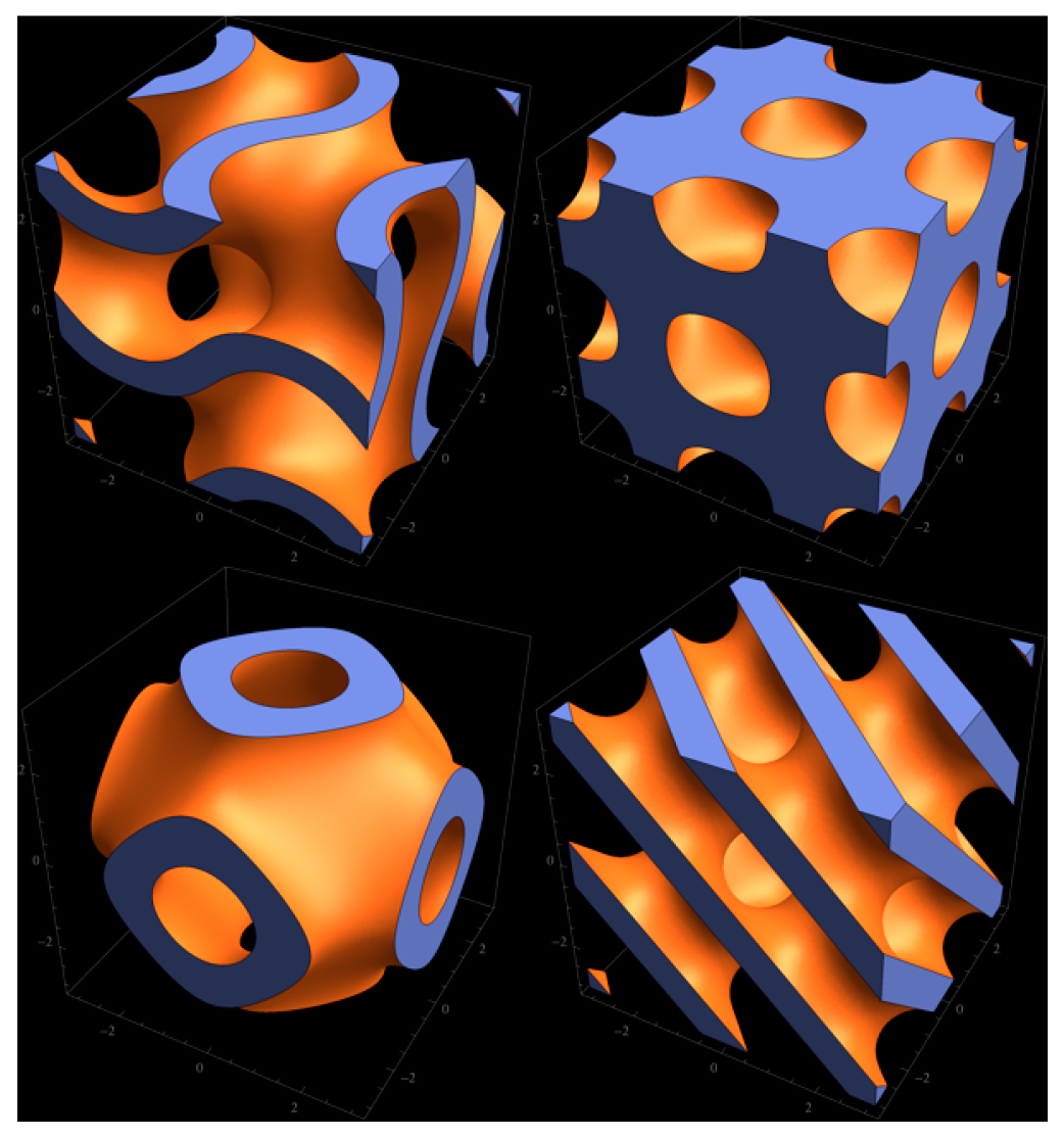
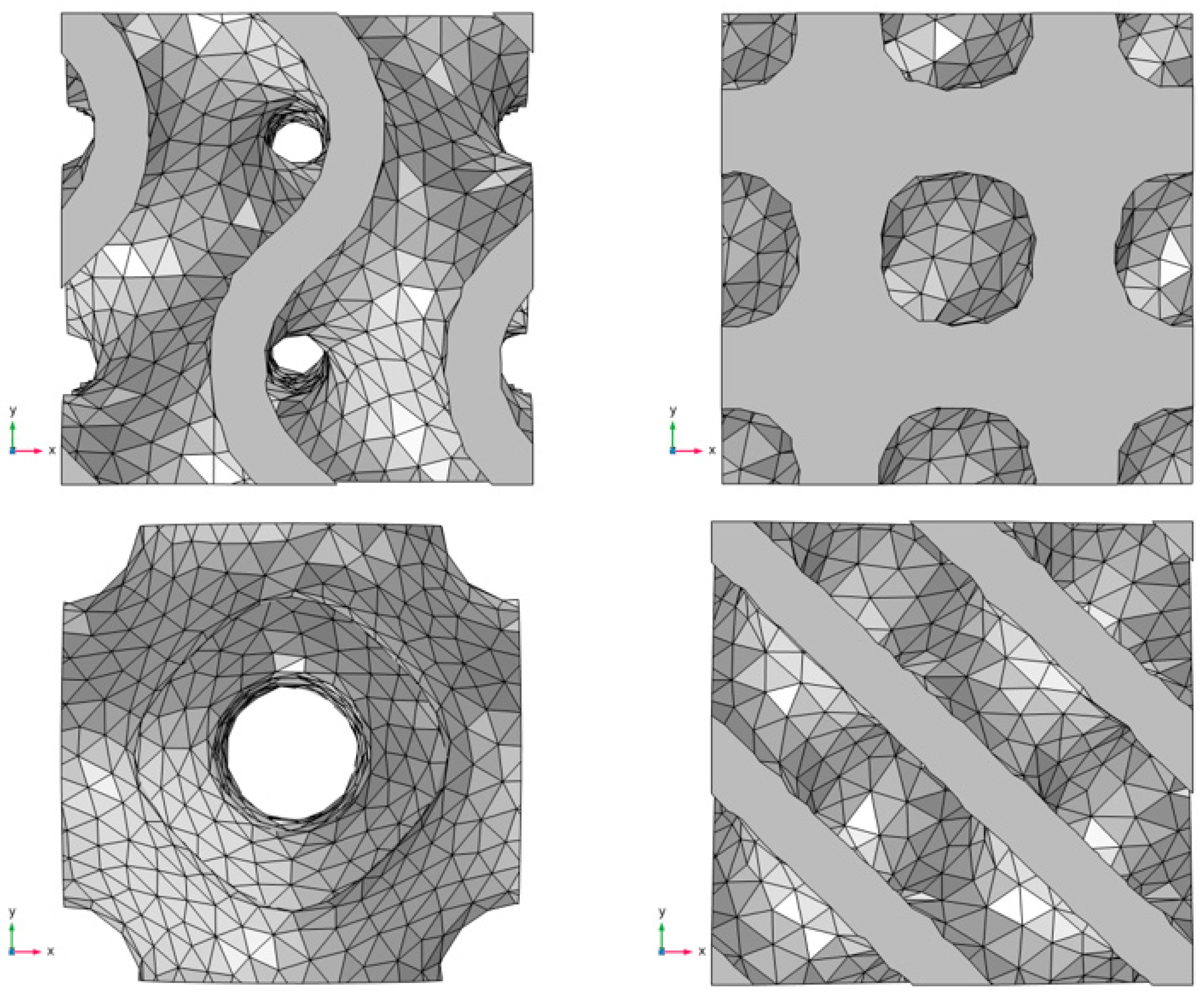
4.1. Controllability Construction of TPMS

Taking a G-type structure as an example, illustrate the process of generating the TPMS using generative equations in Mathematica 12, with a $c$ value ranging from −0.5 to 0.5. The implicit function generation equation of the G structure takes 2π as a period. In order to generate 1 × 1 × 5 TPMS in subsequent microstructures, the initially generated TPMS structure needs to be redundant. The x and y directions are prepared in two periods, and the range of x and y is −2π–2π. Prepare in six cycles in the z-direction, with a range of −7π–7π for z. After generating a 2 × 2 × 7 structure in Mathematica, use the Export command [“filename. stl”, % index] to export the STL format. The STL format file only describes the surface geometry of the 3D object without color, material mapping, or other common 3D model properties.

The structural result generated by Mathematica is shown in Figure 1. The blue part represents the generated TPMS, and the yellow part is the TPMS wall surface.

STL files are discrete triangular mesh descriptions, and their correctness depends on the underlying topological relationships within them. Due to the inherent complexity of the triangle mesh fitting algorithm for solid surfaces, there may be some errors in the output of complex STL files by general modeling systems. So, in order to use the generated structure, some preprocessing repairs are needed.

SpaceClaim 2021 R2 can be invoked within ANSYS Workbench 2021 R2. It serves as ANSYS’s preprocessing software and is ideal for modifying CAD models in CAE simulations.

Select the geometric structure in the component system of Workbench, and select the TPMS structure in STL format opened in SpaceClaim, as shown in Figure 2.

Firstly, use the panel tab to check the facets, which may result in issues such as mesh non-watertightness.

To solve the grid problem, normalization is first performed in SpaceClaim, followed by automatic patch repair operations. After the repair, the patches are converted into STP format entities and exported.

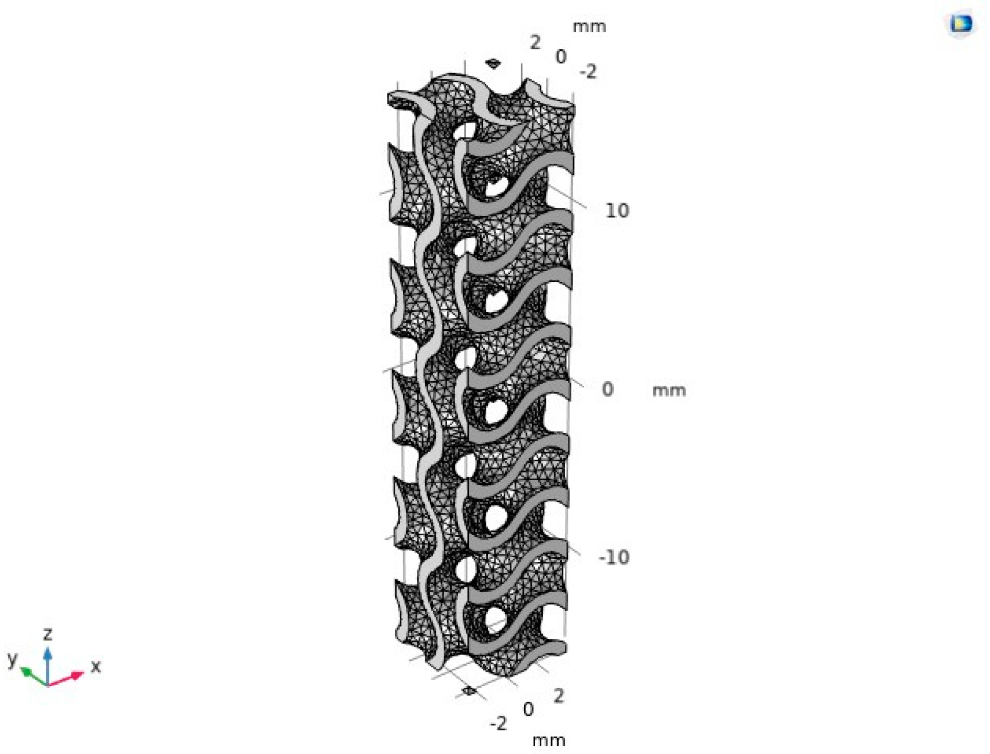
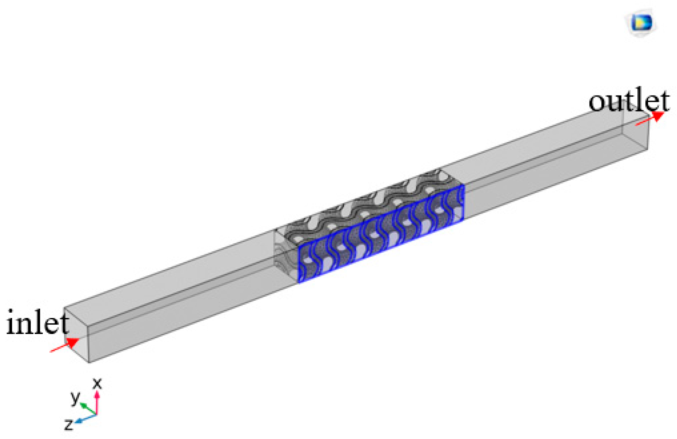
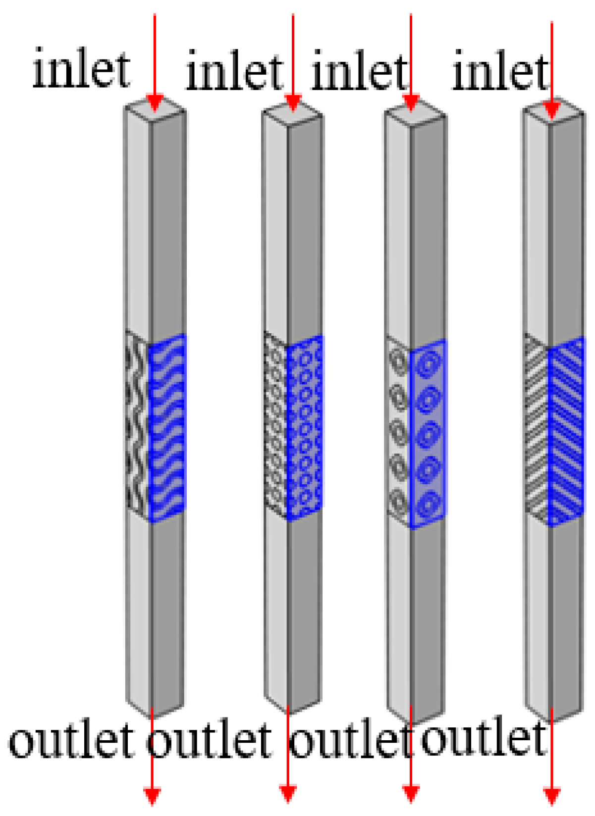
4.2. The Construction Method of Fluid Heat Transfer Model for TPMS Microstructure

Import the STP file generated in the previous section into COMSOL, as shown in Figure 3.

It comes with refined meshes generated by ANSYS Workbench. Observing the imported structure, although it has been processed by the professional grid repair software SpaceClaim, there are still grid defects on the surface of the TPMS, as indicated by the red circle in Figure 4. Therefore, in order to perform subsequent numerical simulations, it is necessary to cut out TPMS structures that conform to the shape.

First, embed an inscribed rectangular prism with an x-axis range of −π–π, a y-axis range of −π–π, and a z-axis range of −5π–5π into the imported COMSOL structure, as shown in Figure 5. The blue color represents the embedded rectangular prism.

Remove the peripheral edge small structures of the G-shaped structure and intersect the main body of the G-shaped structure with the embedded rectangular prism through Boolean operation to obtain the required 1 × 1 × 5 TPMS structure, as shown in Figure 6.

On this basis, the following model is constructed: the left is the fluid inlet, the right is the fluid outlet, and the blue surface is the constant temperature surface at 100 °C, as shown in Figure 7.

The overall size of the model is 2π (mm) × 2π (mm) × 34π (mm). The model is divided into three parts, from top to bottom: a rectangular fluid inlet section, a G-shaped TPMS structure section, and a rectangular fluid outlet section. The dimensions of the three parts are 2π (mm) × 2π (mm) × 12π (mm), 2π (mm) × 2π (mm) × 10π (mm), and 2π (mm) × 2π (mm) × 12π (mm). The presence of the fluid inlet and outlet sections is to avoid boundary effects, which will affect the streamline distribution of the fluid field [34].

When the inflow velocity is 0.01 m/s, the Reynolds number $Re$ of the fluid at the inlet is as follows [35]:

$$Re={\displaystyle \frac{\rho \left|\overrightarrow{u}\right|d}{\mu }}$$

(13)

In the formula, $\left|\overrightarrow{u}\right|$ is the fluid velocity, $d$ is the characteristic length, which is the equivalent diameter side length of a cube for a cross-section [36], μ is the dynamic viscosity coefficient of the liquid and its value is $0.001Pa\times s$, and the Reynolds number characterizes the magnitude of the viscous force. According to the criteria for determining the Reynolds number, $Re$ < 2300 indicates that the fluid is laminar, which is the basis for selecting laminar flow in COMSOL.

Similarly, with a $c$ value range of −0.5–0.5 and equal cell volumes, establish physical models for D-type and P-type structures. Below is an overview of the four structural models. The unit structures shown in Figure 8, from left to right and from top to bottom, are sheet-like TPMS cells of G, D1, P, and D2, respectively.

The structure of 1 × 1 × 5 imported into COMSOL for the above four units is shown in Figure 9.

The further generated microstructure models of G, D1, P, and D2 are shown in Figure 10.

For TPMS, porosity $\varphi$ is its essential parameter, which can reflect the proportion of solid materials inside the structure. Porosity refers to the ratio of the total volume of pores within the TPMS structure to the total volume of the TPMS, and its calculation formula is as follows [37]:

$$\varphi =\left({\displaystyle \frac{V_f}{V}}\right)=\left({\displaystyle \frac{V_f}{V_f+V_s}}\right)$$

(14)

In the formula, $V$ represents the total volume of the porous structure, $V_f$ represents the total volume of the pores within the porous structure, and $V_s$ represents the total volume of the solid portion within the porous structure.

Develop code for calculation which reflects the volume proportion by extracting points from the design structure. Because a homogeneous TPMS structure is composed of multiple TPMS units, adding an identical TPMS unit increases the pore volume and total volume of the entire structure proportionally. Therefore, the porosity of a homogeneous structure is consistent with that of a single unit. Mathematically speaking, if the pore volume of the TPMS unit is $V_{f0}$ and the total volume of the units is $V_0$, then the total pore volume of the structure containing $m$ TPMS units is $m{V}_{f0}$, and the total volume of the units is $m{V}_0$. Their porosity is the same:

$${\varphi }_0=\left({\displaystyle \frac{V_{f0}}{V_0}}\right)=\left({\displaystyle \frac{{mV}_{f0}}{m{V}_0}}\right)$$

(15)

Directly calculate the porosity of a single unit with a length of 2π.

Use the Flatten function to extract points from the TPMS within the range of −4π–4π for x, y, and z, with an accuracy of 0.05, denoted as point0. Define point1 as a point with a $c$ value between −0.5–0.5, representing the points in the TPMS generated by the implicit function. The specific expression is as follows:

$$point1=Select\left[point0,-0.5<c<0.5\right]$$

(16)

The porosity $\varphi$ is as follows:

$$\varphi =1-N\left({\displaystyle \frac{Length\left[point1\right]}{Length\left[point0\right]}}\right)$$

(17)

Calculate the solid proportion of the four structures in contact with the constant temperature surface and the porosity of the TPMS part; the results are shown in

Table 1. Surface Solid Proportion, Porosity and SSA.

Type	Gyroid	Diamond 1	Primitive	Diamond 2
Constant temperature surface area (mm2)	197.39	197.39	197.39	197.39
Solid contact area (mm2)	55.166	127.800	44.442	67.682
Solid proportion	27.95%	64.74%	22.51%	34.29%
Porosity	67.65%	41.45%	71.45%	58.87%
SSA (m−1)	2.923	1.731	1.886	2.652

. The initial and boundary conditions of the model are shown in

Table 2. Initial Boundary Conditions.

Type	Gyroid	Diamond	Primitive
Inlet velocity (m/s)	0.01–0.11	0.01–0.11	0.01–0.11
Structural outlet pressure (Pa)	0	0	0
Constant temperature wall (K)	373.15	373.15	373.15
Excluding the surrounding walls of the constant temperature wall	Thermal insulation	Thermal insulation	Thermal insulation
Fluid wall conditions	No slip	No slip	No slip
TPMS initial temperature (K)	293.15	293.15	293.15
Inlet fluid temperature (K)	293.15	293.15	293.15

, where “excluding the surrounding walls of the constant temperature wall” refers to the other sides beside “inlet, outlet, constant temperature wall”.

The entrance speed is set to 0.01–0.11 m/s, with a step size of 0.02 m/s.

Regarding material selection, 316 L stainless steel is chosen for the solid part, and water is chosen for the liquid part, both of which have inherent properties in COMSOL. Use a steady-state solver when solving.

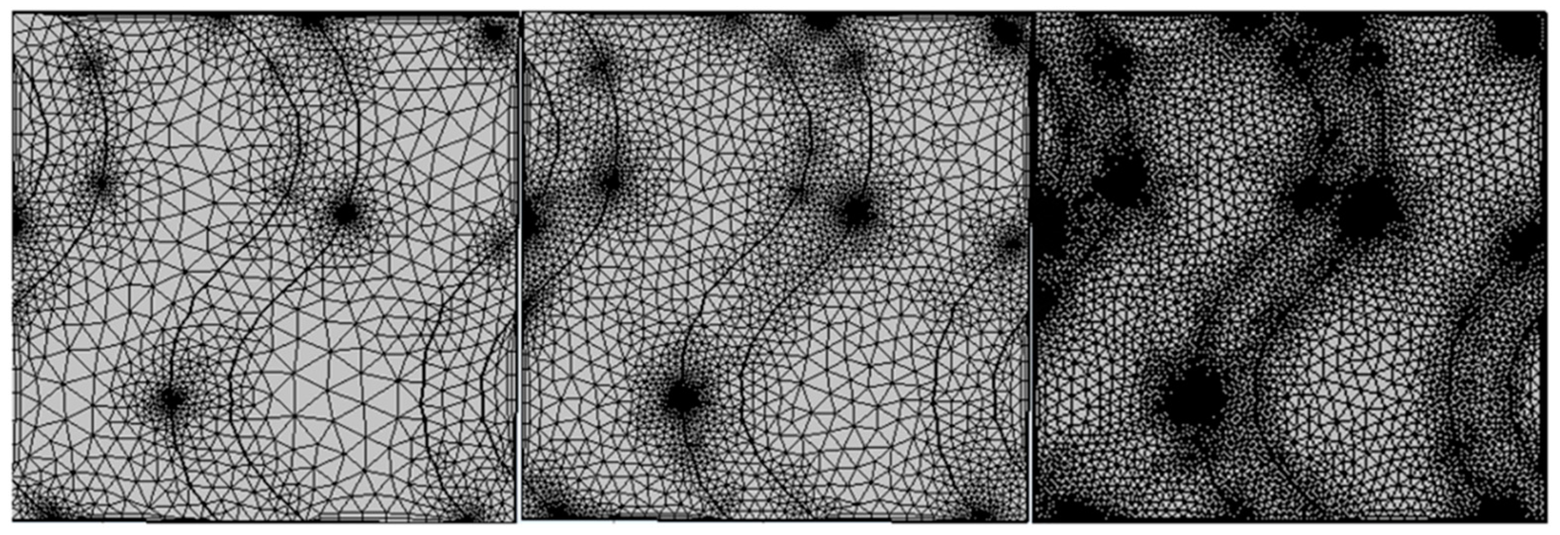
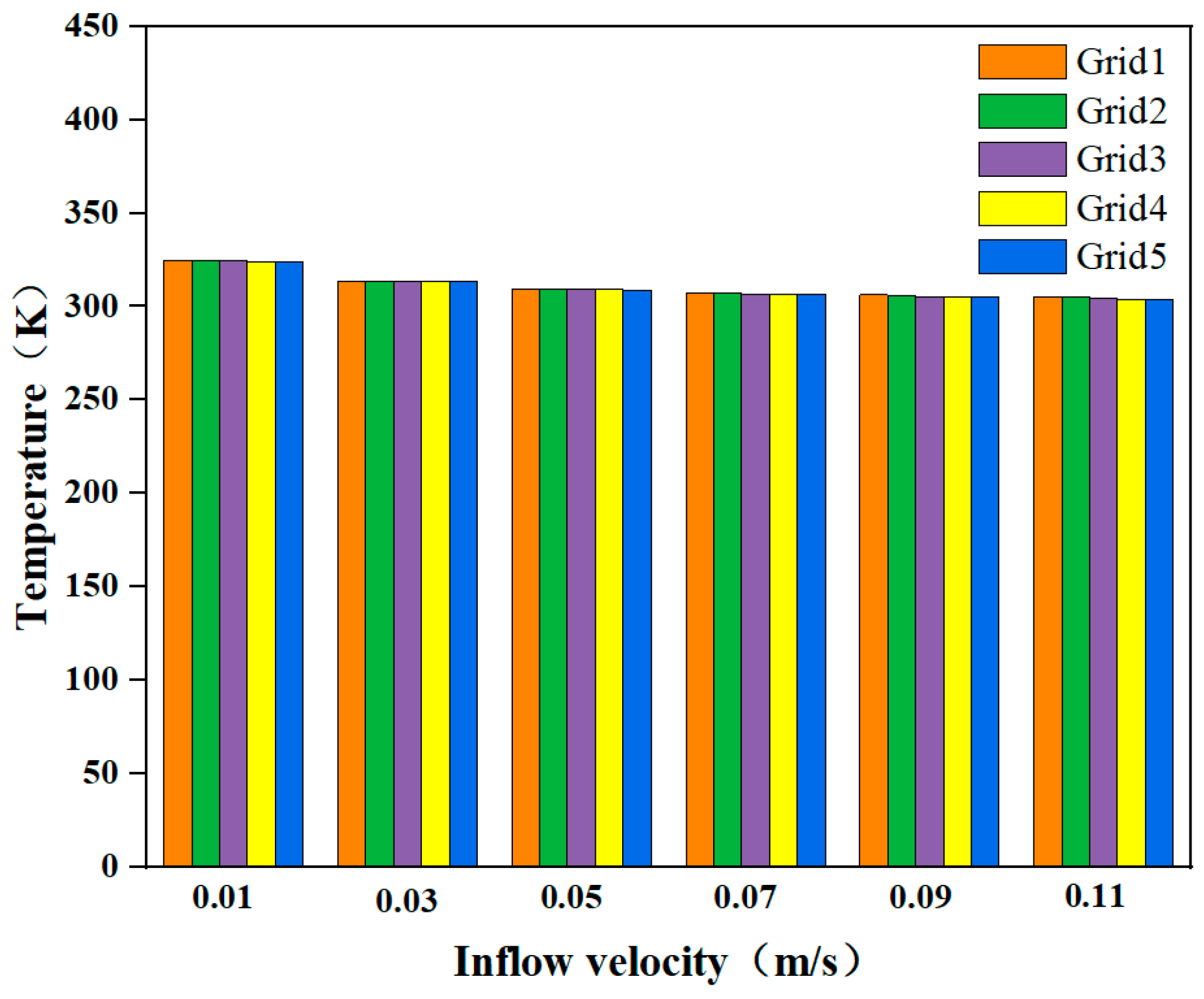
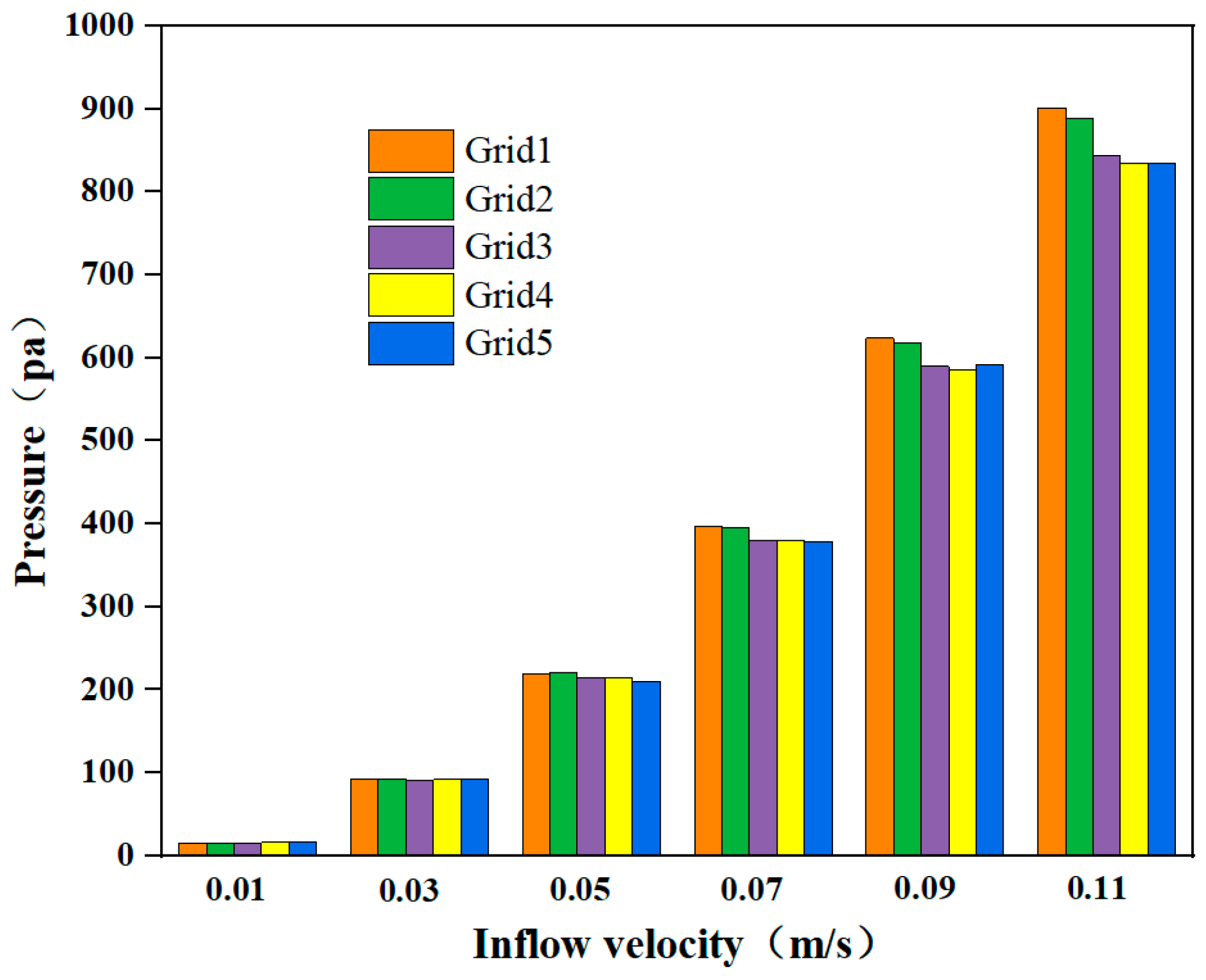
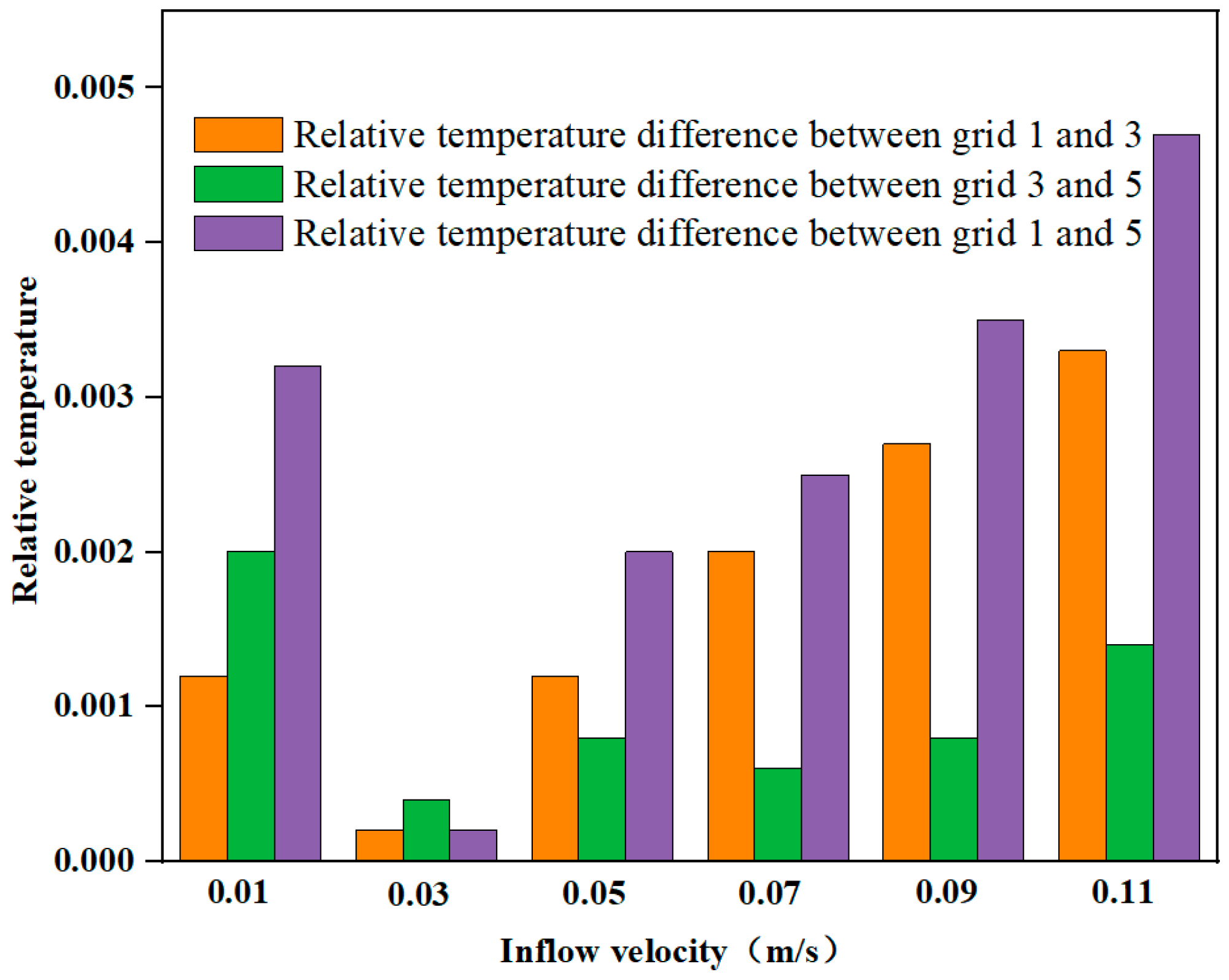
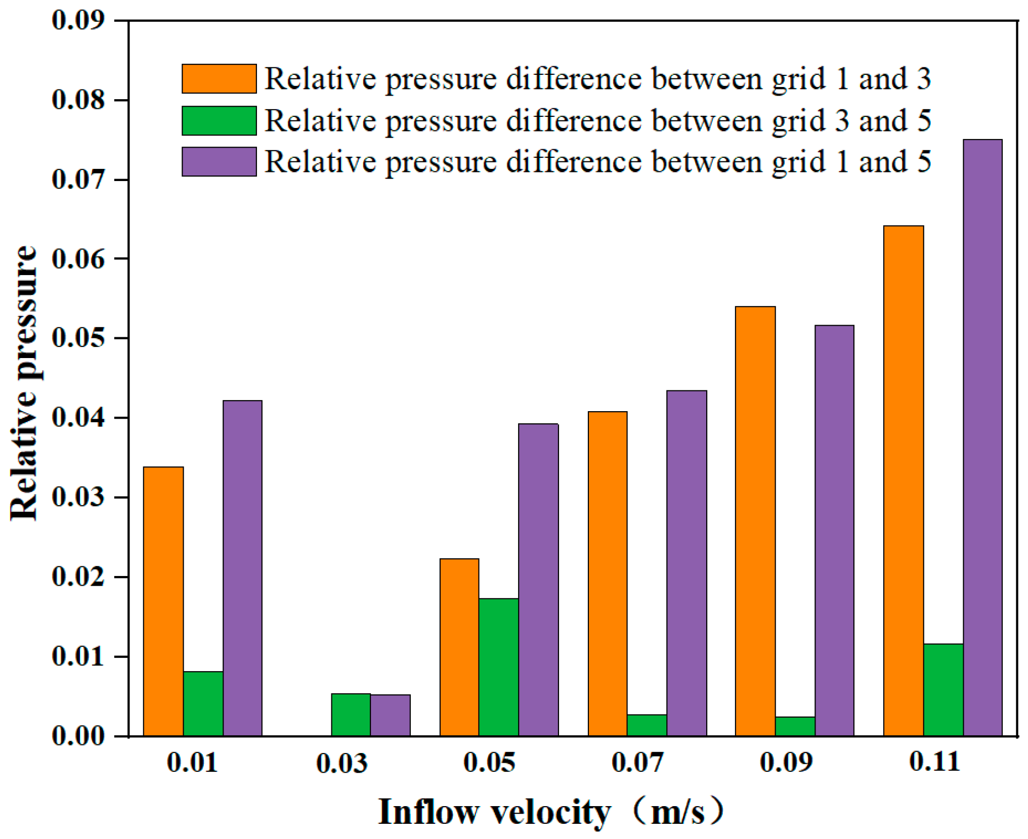
4.3. Grid Independence Test

Taking the example of the Gyroid microstructure at a wall temperature of 100 °C and an inlet flow velocity of 0.01–0.11 m/s, the grid independence verification is carried out. The grid adopted from coarse to fine is shown in the

Table 3. Number of grids and computation time.

	Grid 1	Grid 2	Grid 3	Grid 4	Grid 5
Number of grids	813,898	953,449	2,174,127	3,977,522	6,519,047
Computing time	58 min	1 h 50 min	2 h 51 min	13 h 15 min	16 h 44 min

.

Display the mesh division of different refinement levels on the entrance surface of the microstructure TPMS, as shown in the Figure 11 for grid 1, 3, and 5.

Figure 12, Figure 13, Figure 14 and Figure 15 show the results of different grid calculations.

From the perspective of relative difference, the difference between grid 1 and grid 3 is based on grid 1. The difference between grid 3 and grid 5 is based on grid 3, and the difference between grid 1 and grid 5 is based on grid 1. From Figure 14, the maximum temperature difference in the entire calculation does not exceed 0.5%. From Figure 15, the maximum difference in pressure values between grid 1 and grid 5 is 7.5%, not exceeding 10%, with a relative multiple of 1.08 times from Figure 13. After an inlet flow rate of 0.05 m/s, as the number of grids increases, the the difference between temperature and pressure calculations decreases from Figure 12 and Figure 13. Therefore, the grid independence test has been confirmed. This study has high computational costs (CPU time and memory), and, based on current computing resources, we have chosen to perform calculations according to grid 1. The difference in the maximum grid size among the five types is 4.99 times and the average cell quality of the roughest grid is 0.6317, which meets the simulation requirements.

4.4. Flow and Heat Transfer Processes in TPMS Microfluidic Heat Transfer Model

In order to select and construct macroscopic TPMS microstructures, it is necessary to analyze and compare the flow and heat transfer processes of the three microstructures.

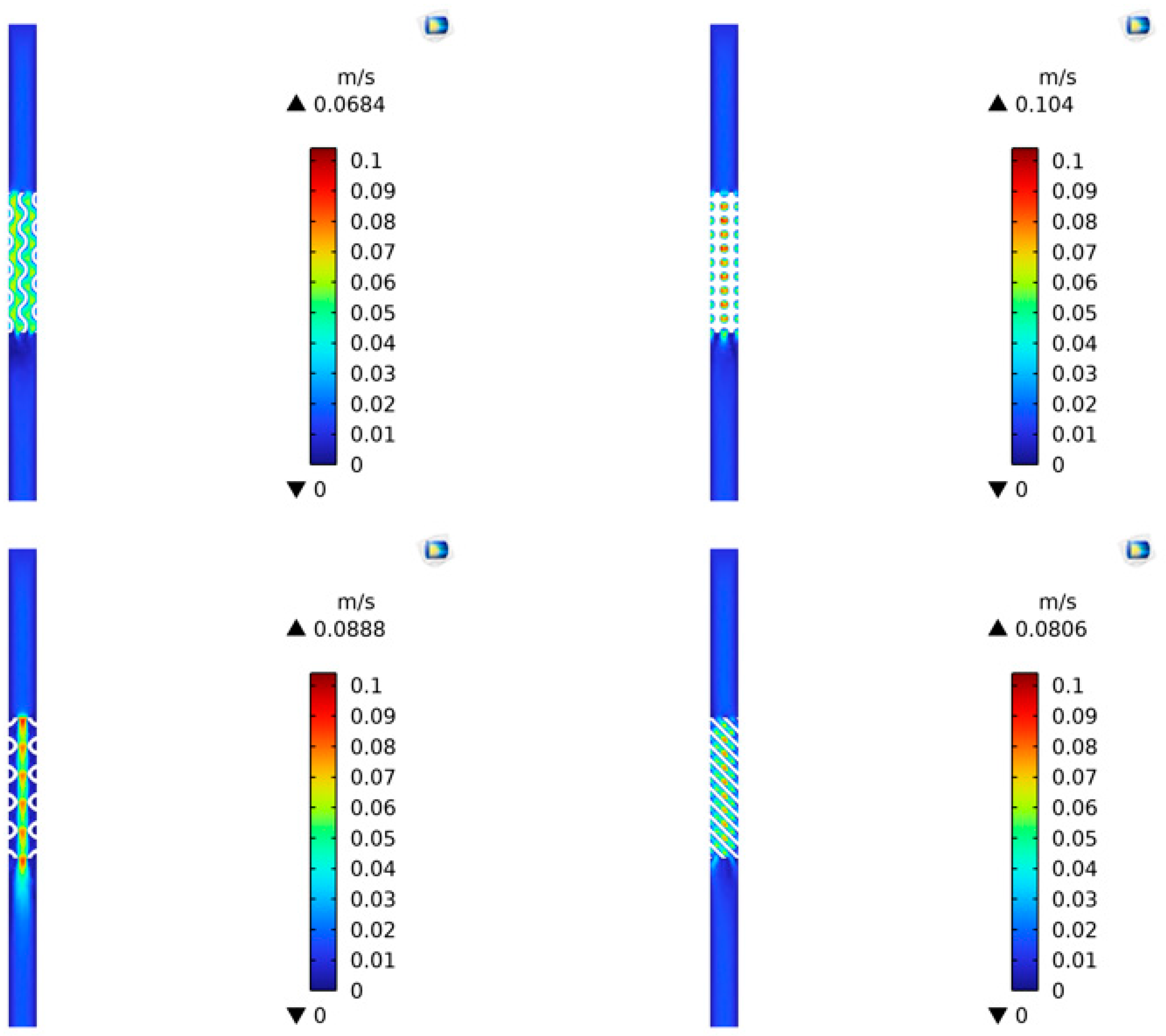
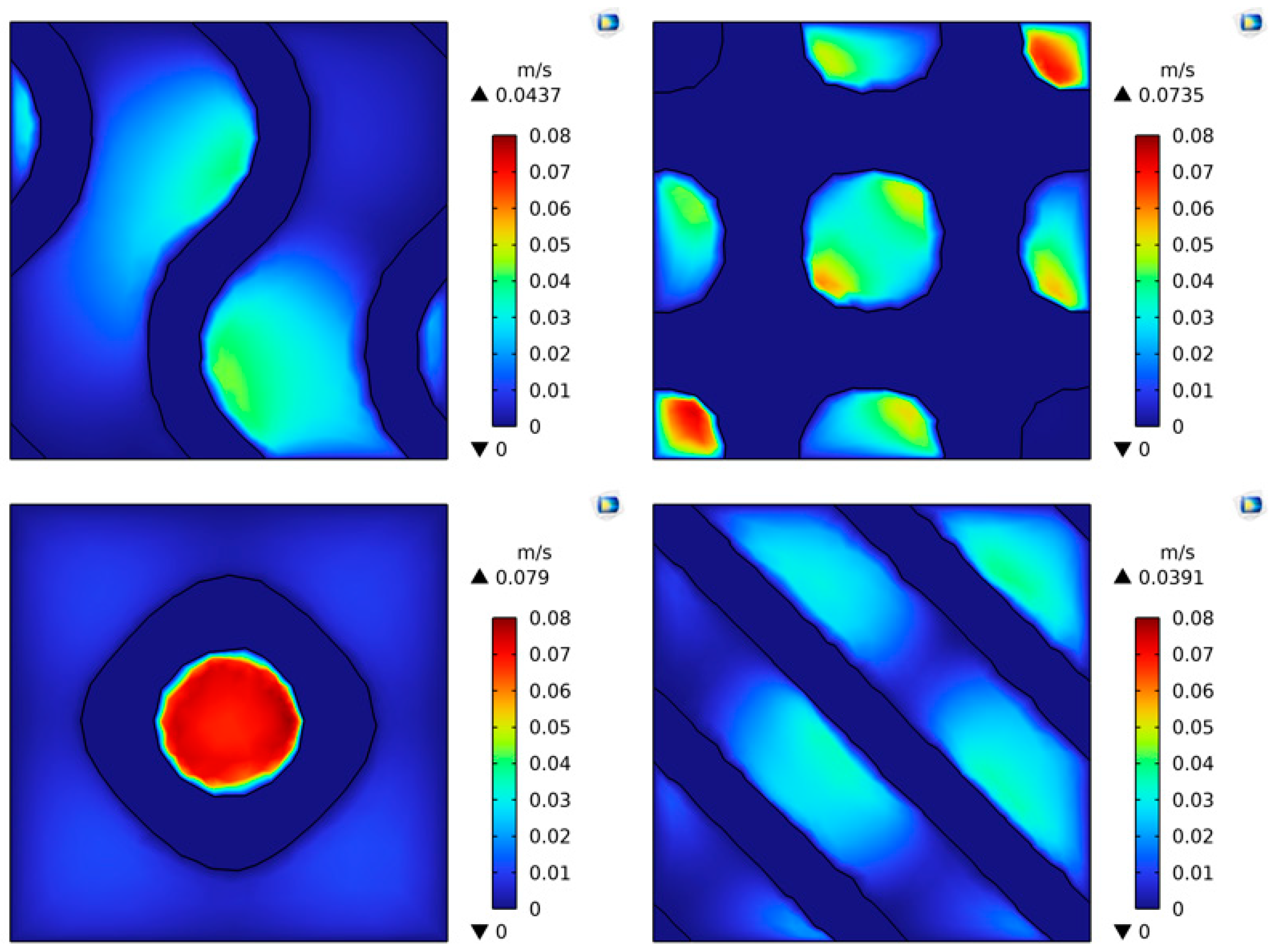
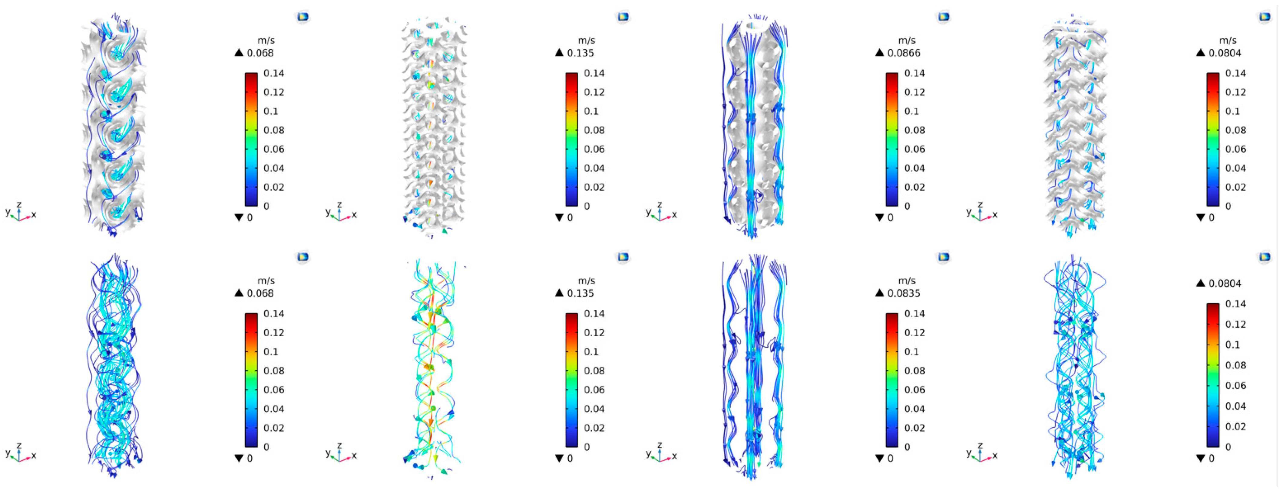
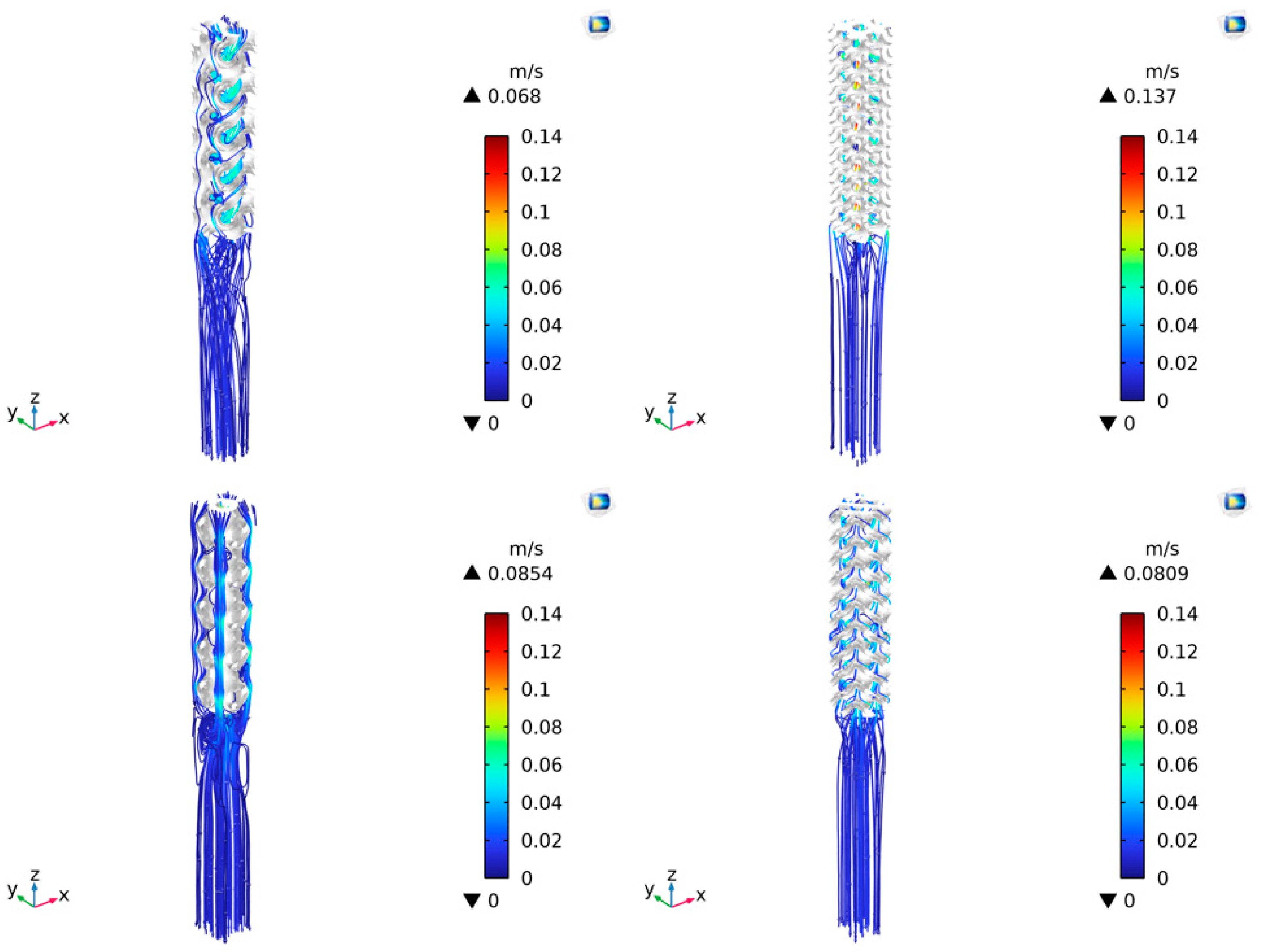
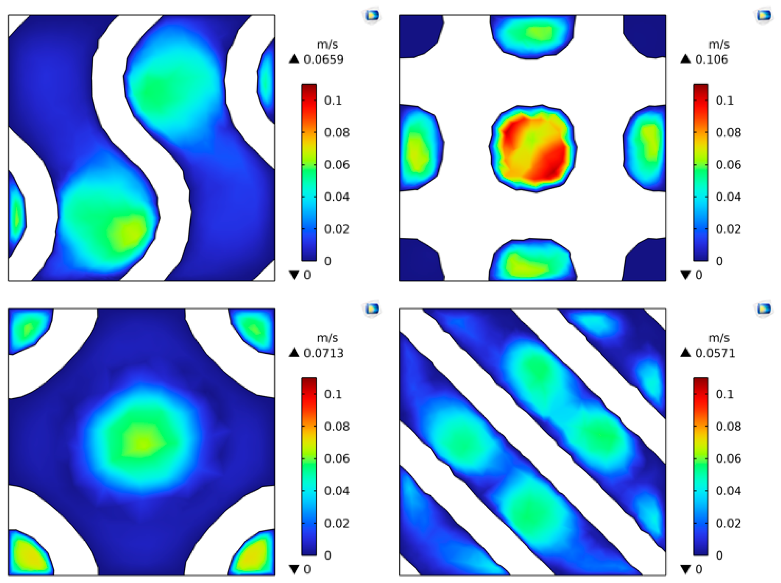
4.4.1. Flow Characteristic

Comparing the flow process, with an inlet velocity of 0.01 m/s, the three-dimensional sectional flow velocities of G, D1, P, and D2 structures are shown in Figure 16. It can be observed that the TPMS part has a significant increase in flow velocity relative to the fluid inlet section.

Observing the yz section with x = 0, the flow velocity of the TPMS increases more significantly relative to the fluid inlet section, as shown in Figure 17. This is determined by the continuity of fluid mechanics. According to the conservation of mass equation, the mass of the fluid flowing into the interface between the inlet section and the TPMS is equal to the mass flowing out of this section. Moreover, due to the small longitudinal length of the fluid on both sides of this section, the density change is minimal, indicating that the flow velocity on both sides of the section is inversely proportional to the cross-sectional area of the respective fluids. Therefore, the flow velocity of the TPMS section with a smaller fluid area is significantly increased compared to the inlet and outlet sections of the fluid. This is similar to the narrow pipe effect in geography.

To demonstrate the correctness of the above understanding, the pore and velocity characteristics of the cross-section at the interface between the fluid inlet section and TPMS were extracted. It is shown in Figure 18 and

Table 4. Proportion of liquid at the entrance surface of microstructure TPMS.

Type	Gyroid	Diamond 1	Primitive	Diamond 2
Maximum velocity (m/s)	0.0437	0.0735	0.079	0.0391
Average velocity (m/s)	0.0134	0.0255	0.0121	0.0148
Liquid area (mm2)	28.466	13.933	30.517	25.796
Proportion of liquid	72.11%	35.29%	77.30%	65.34%

.

The fluid velocity is continuous on both sides of the cross-section. The average flow velocity is calculated based on the fluid domain at the inlet of the TPMS section. As shown in Table 4, the average flow velocity is negatively correlated with the fluid area at the inlet section of the TPMS; the average flow velocity is D1 > D2 > G > P.

The velocity cloud map of the yz section along the fluid flow direction for G, D, and P-type structures is shown in Figure 19. Among them, the maximum flow velocity of the G-type, D2-type, and P-type structures is lower than that of the D1 structure. From Table 1, it can be seen that the porosity of the D1 structure is the smallest. Additionally, from a separate section, it can also be observed that the proportion of D1 fluid is relatively smaller compared to the other three structures. With a lower porosity and smaller cross-sectional area occupied by pores, it is more likely to generate higher velocities.

To understand the physical mechanisms involved in the flow process and analyze the microstructure streamline characteristics, observe the structure of the TPMS along the mainstream direction from Figure 20. The D1 and D2 structure has no through holes, making the flow more complex and easier to be drained by the structure. The through holes of both G and P structures have obvious main flow, while the D1 and D2 structures have more vortices and secondary flow in the TPMS where the fluid is diverted, and have a thinning effect on the boundary layer.

The four essential streamline structures extracted are shown in Figure 21 and Figure 22.

As shown in Figure 23, the outflow part of G has a streamline deviation. The streamline on the side closer to the constant temperature surface in the TPMS is located on the side farther away from the heating in the outlet section, resulting in the high-temperature area at the outlet not being close to the constant temperature surface side. There is a secondary flow in G. As shown in Figure 22 and Figure 23, the fluid in the P-type structure is less obstructed, and there is a significant secondary flow and vortex at the outlet of the TPMS; a flow dead zone has formed here which is unfavorable for heat transfer. From Figure 21, Figure 22 and Figure 23, the flow paths of G and D surfaces are more complex, and these two structures can generate strong helical motion in the direction of water flow. These eccentric motions can squeeze the thermal boundary layer, thereby enhancing fluid mixing and removing residues in the channel [38].

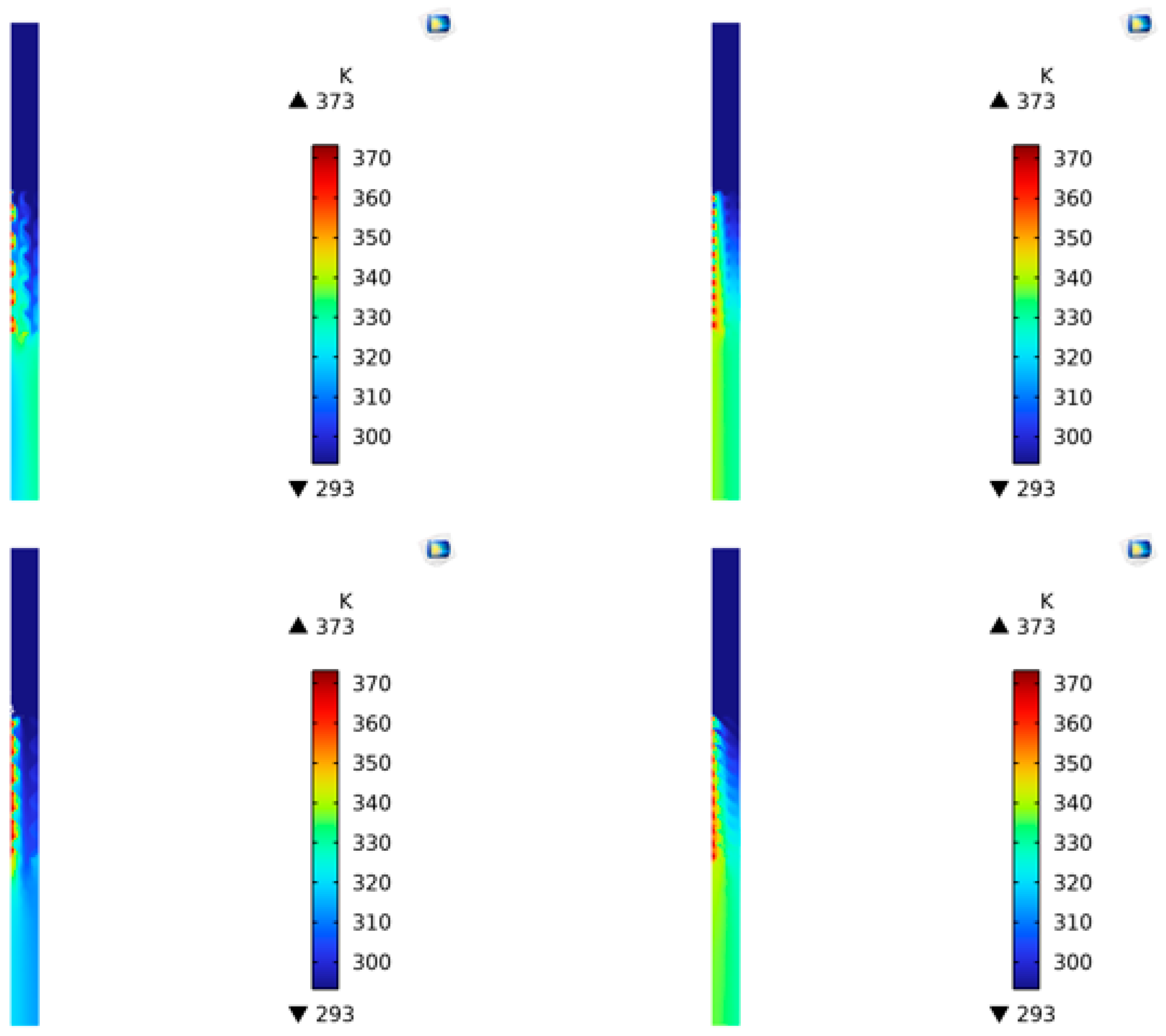
4.4.2. Heat Transfer Characteristics

At the xy, z = 0 section of the TPMS, the velocity and temperature distributions of the four structures are as follows: compared to the entrance of the TPMS, except for the P-type, the maximum velocity of the other three structure sections has increased. Its velocity cloud map is show in Figure 24.

Its temperature cloud map is shown in Figure 25; when reaching a steady state, the lowest temperature of the D1 structure is 309 °C, the highest among the four structures. This is because the area proportion of the solid part in contact with the constant temperature surface of the D1 structure is the largest among the four structures. Referring to Table 1, the lowest temperature ranking of the other three structures is also positively correlated with the area proportion of the solid part, that is, D1 > D2 > G > P.

In the yz, x = 0 section of the TPMS, and the temperature distribution of the four structures in Figure 26 is as follows: along the y direction, the temperature inside the TPMS changes more dramatically.

In the range of inlet flow velocity from 0.01 m/s to 0.11 m/s, corresponding to Reynolds numbers of 20π–220π, to determine the performance of the structure, it is necessary to analyze the outlet temperature and pressure of the microstructure. The relationship between them and velocity is shown in the following

Table 5. Outlet temperatures of four microstructures at different flow rates.

Name	Inlet Velocity	G Microstructure Outlet Temperature	D1 Microstructure Outlet Temperature	P Microstructure Outlet Temperature	D2 Microstructure Outlet Temperature
Unit	m/s	K	K	K	K
	0.01	324.84	334.14	317.00	333.19
	0.03	313.29	318.55	308.28	317.99
	0.05	309.47	313.71	305.73	313.09
	0.07	307.49	311.16	304.37	310.80
	0.09	306.27	309.55	303.49	309.40
	0.11	305.44	308.43	302.86	308.40

and

Table 6. Pressures of four microstructures at different flow rates.

Name	Inlet Velocity	G Microstructure Pressure	D1 Microstructure Pressure	P Microstructure Pressure	D2 Microstructure Pressure
Unit	m/s	Pa	Pa	Pa	Pa
	0.01	15.34	100.51	13.52	28.89
	0.03	91.78	762.06	86.33	163.66
	0.05	219.11	2025.20	211.82	381.70
	0.07	396.21	3882.90	386.62	678.19
	0.09	623.33	6324.70	610.74	1052.70
	0.11	901.02	9346.10	884.26	1505.90

and Figure 27 and Figure 28; when the inlet flow velocity is the same, the outlet temperature of the D1 and D2 structures is equivalent and higher than that of G and P structures, indicating that the D structure has more robust heat transfer. At the same time, as the inlet flow velocity increases, the outlet temperature of each structure decreases, and the maximum temperature difference of each structure within the research range decreases from 17.14 °C to 5.56 °C. For the same flow velocity, a structure with a higher outlet temperature indicates that this structure has more heat exchange and stronger heat transfer capacity. For the same structure, an increased inlet flow velocity will increase the rate of flow of cold fluid through the structure, thereby reducing the outlet temperature.

In liquid cooling systems, pressure is an important variable. In general, for the same structure, as the flow velocity increases, the system’s heat dissipation capacity increases, and the corresponding pressure also increases, resulting in the need for a more powerful pump to transport the liquid into the structure. So, it is necessary to pay attention to pressure when studying liquid cooling heat dissipation systems. From Figure 28, as the inlet flow velocity increases, the system pressure of all four structures increases, and their growth trend D1 is much greater than D2 and it can be seen that the pressure of the D1 structure is much higher than the other three structures, so in terms of structural performance, D2 is superior to D1. At the same time, the pressure of G and P is lower than that of the D2 structure and very close; that is, the performance of G and P pressure is better than D2. Taking a flow velocity of 0.11 m/s as an example, D2 has a pressure of 1505.9 Pa, G has a pressure of 901.02 Pa, and P has a pressure of 884.26 Pa; the pressure of D2 is 1.67 times that of G, with a pressure difference of 604.88 Pa; the pressure of D2 is 1.70 times that of P; and the pressure difference is 621.64 Pa.

5. Numerical Simulation Evaluation of Convective Heat Transfer Performance of the TPMS Microstructure

Calculating the convective heat transfer coefficient, Nusselt number, and wall friction factor is necessary to evaluate heat transfer performance and pressure drop loss.

The average convective heat transfer coefficient represents the amount of heat exchanged per unit of wall area and fluid per unit of time when the temperature difference between the fluid and the wall is 1 °C. Its magnitude indicates the strength of convective heat transfer. The Nusselt number is a dimensionless parameter that characterizes a fluid’s convective heat transfer intensity, reflecting the comparative relationship between the heat transfer capacity between the fluid and the wall of a given heat transfer system and the thermal conductivity of the fluid. The average wall friction factor reflects the power loss of the radiator. In this structure, the average convective heat transfer coefficient $h_0$ is determined by Equation (18) [19], and the Nusselt number $Nu$ [20,33] and the average wall friction factor $f$ are determined by Equations (19) and (20) [17]:

$$\rho \left|\overrightarrow{u}\right|A_0{C}_p∆T=h_0{A}_1\left(t_w-t_f\right)$$

(18)

$$Nu={\displaystyle \frac{h_{0}d}{k}}$$

(19)

$$f={\displaystyle \frac{2pd}{\rho {\left|\overrightarrow{u}\right|}^2{L}_0}}$$

(20)

The Equation (18) represents the conservation of energy in the system and indicates that the increase in structural temperature is due to the heat exchange between the fluid and the isothermal surface. In the formula, $A_0$ is the inlet area, $C_p$ is the specific heat capacity of water, $∆T$ is the temperature difference between the outlet and inlet of the structure, $A_1$ is the outlet area, $t_w$ is the temperature of the constant temperature wall, and $t_f$ is the qualitative temperature of the fluid. Here, it is taken as follows: $t_f={\displaystyle \frac{t_{in}+t_{out}}{2}}$, where $t_{in}$ is the inlet temperature and $t_{out}$ is the outlet temperature. In the Equations (19) and (20), $d$ is the hydraulic diameter, $k$ is the thermal conductivity of water, $p$ is the pressure of the structure, and $L_0$ is the length of the flow channel. In steady state, the values of various physical property parameters need to be calculated based on qualitative temperature.

The relationship between velocity and average convective heat transfer coefficient $h_0$, Nusselt number $Nu$, and average wall friction factor f obtained from post-processing is shown in

Table 7. Average convective heat transfer coefficients $h_0$ of four microstructures at different flow velocities.

Name	Inlet Velocity	$\mathbf{G}-{\mathit{h}}_0$	$\mathbf{D}1-{\mathit{h}}_0$	$\mathbf{P}-{\mathit{h}}_0$	$\mathbf{D}2-{\mathit{h}}_0$
Unit	m/s	W/(m2·K)	W/(m2·K)	W/(m2·K)	W/(m2·K)
	0.01	4105.1	5722.1	2918.5	5549.1
	0.03	7199.8	9429.7	5221.8	9184.7
	0.05	9465.6	12,286	7112.5	11,862
	0.07	11,490	14,796	8803.9	14,465
	0.09	13,401	17,133	10,368	16,958
	0.11	15,264	19,371	11,858	19,315

,

Table 8. Nusselt numbers $Nu$ of four microstructures at different flow velocities.

Name	Inlet Velocity	$\mathbf{G}-\mathit{N}\mathit{u}$	$\mathbf{D}1-\mathit{N}\mathit{u}$	$\mathbf{P}-\mathit{N}\mathit{u}$	$\mathbf{D}2-\mathit{N}\mathit{u}$
Unit	m/s
	0.01	41.350	57.031	29.683	55.368
	0.03	73.577	95.719	53.721	93.297
	0.05	97.224	125.490	73.429	121.260
	0.07	118.330	151.630	91.063	148.310
	0.09	138.250	175.960	107.370	174.190
	0.11	157.650	199.240	122.920	198.670

and

Table 9. Wall friction factors $f$ of four microstructures at different flow velocities.

Name	Inlet Velocity	$\mathbf{G}-\mathit{f}$	$\mathbf{D}1-\mathit{f}$	$\mathbf{P}-\mathit{f}$	$\mathbf{D}2-\mathit{f}$
Unit	m/s
	0.01	18.158	119.25	15.986	34.258
	0.03	12.052	100.17	11.328	21.505
	0.05	10.352	95.755	10.002	18.043
	0.07	9.548	93.628	9.313	16.351
	0.09	9.085	92.235	8.899	15.350
	0.11	8.790	91.225	8.624	14.698

and Figure 29, Figure 30 and Figure 31. As the flow velocity increases, the $h_0$ and $Nu$ of each structure increase while $f$ decreases. That is, within the research range, an increase in flow velocity is beneficial for heat transfer, but it will increase the system’s pressure loss.

From Figure 29, Figure 30 and Figure 31, it can be seen that for $h_0$ and $Nu$, which characterize heat transfer capacity, D1 is similar to D2, and their relationship is D1 ≈ D2 > G > P. The average wall friction factor $f$ D1 is much higher than other structures, and D2 is higher than G and P, which are equivalent to the average wall friction factor. The relationship is D1 > D2 > G ≈ P. At the same time, it can be seen that as the inlet flow velocity increases, $h_0$ and $Nu$ increase, and $f$ declines.

6. Summary and Conclusions

This paper constructs a fluid heat transfer model for the most typical microstructures of G, D, and P in TPMS through geometric modeling using Mathematica, SpaceClaim, COMSOL, mesh repair, and consideration of the inlet section effect of the fluid. By using constant temperature wall heating, the characteristics and differences of flow and heat transfer in various structures were explained by analyzing the proportion of solid area on the constant temperature wall surface, the porosity of the structure, and the distribution of streamlines in the microstructure. The research studied the influence of inlet flow velocity on the outlet temperature $t_{out}$, pressure, $h_0$, $Nu$, and $f$ of the structure, and obtained the following results:

(1)

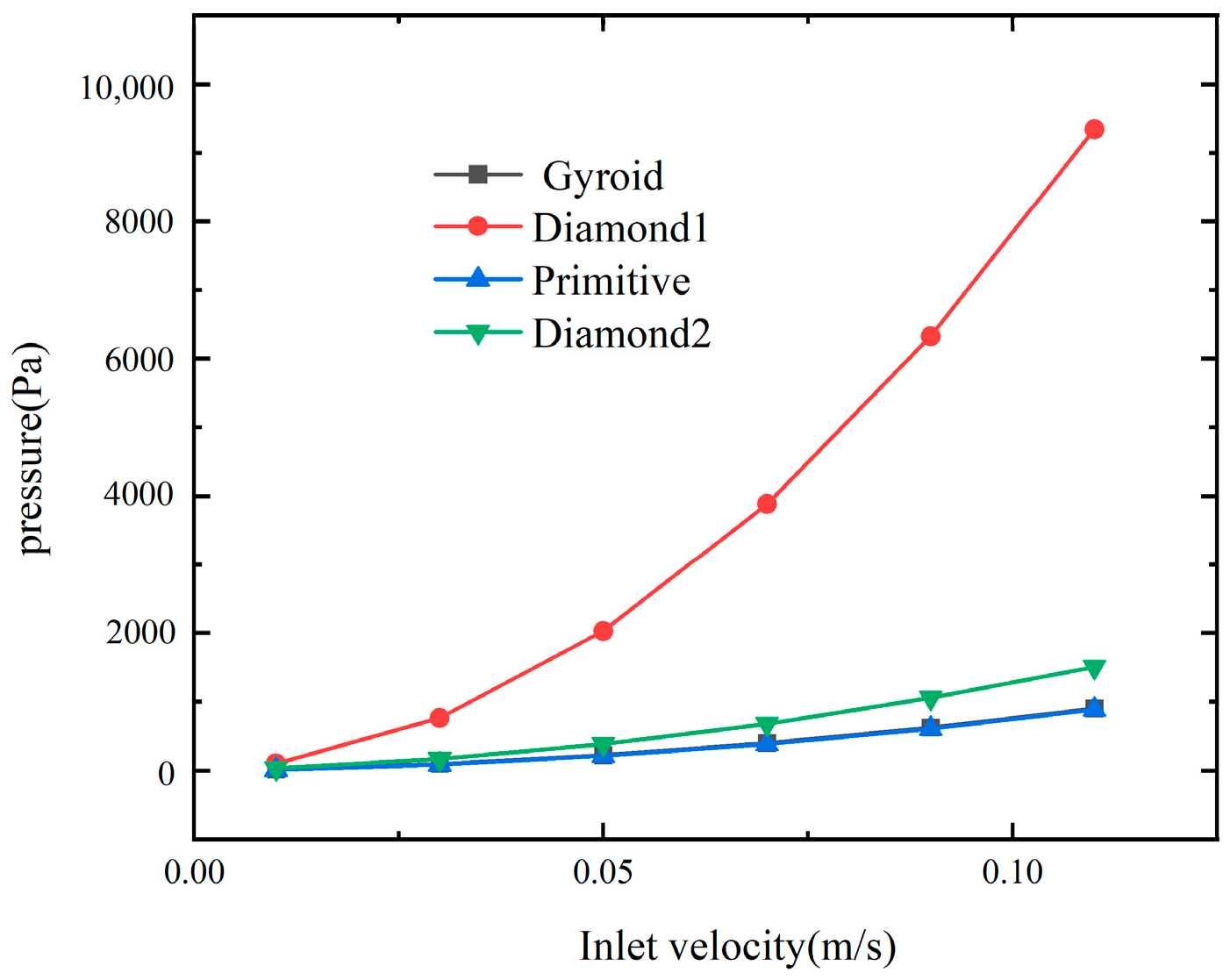
For the same structure, the inlet velocity increases, pressure $p$, $h_0$, $Nu$ increase, and outlet temperature $t_{out}$, $f$ decreases.

(2)

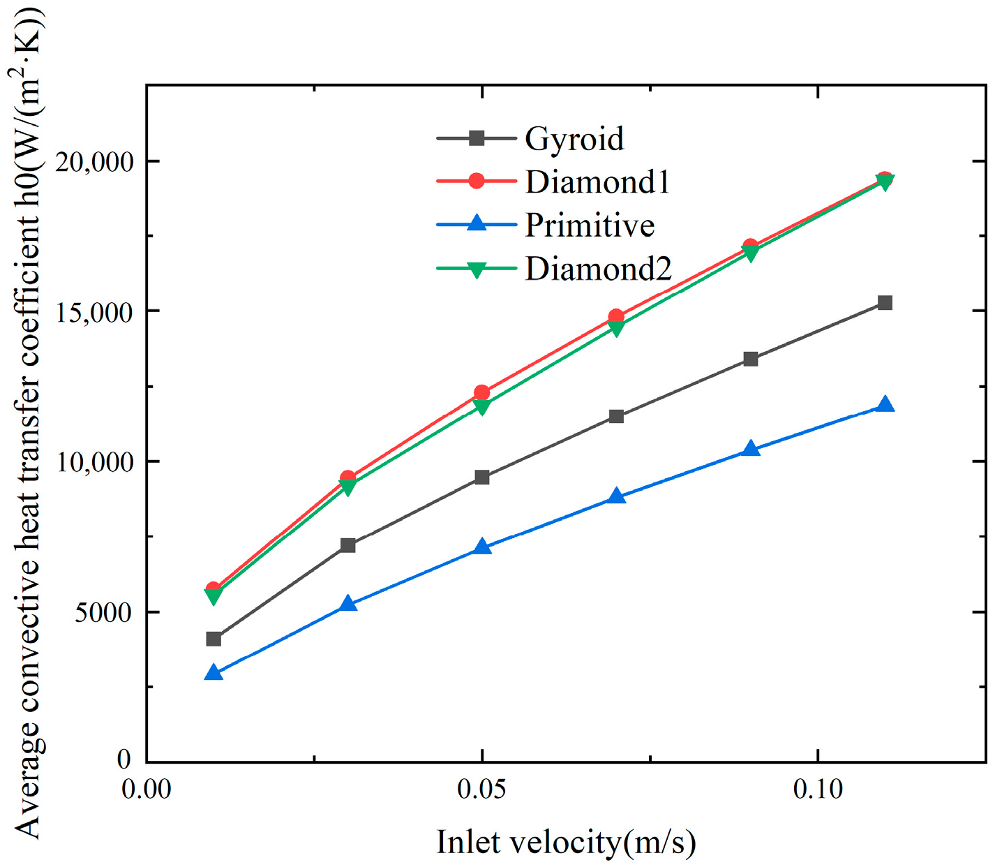
Within the speed range studied in this article, this paper finds that D1 and D2 have similar outlet temperatures $t_{out}$, $h_0$ and $Nu$, but D1’s structural pressure $p$ and average wall friction factor $f$ are far greater than D2. That is, the heat transfer capability is D1 ≈ D2 > G > P. The required power consumption is D1 > D2 > G ≈ P.

(3)

When flow velocity is 0.01 m/s, the maximum temperature difference at the outlet of the four structures reached 17.14 °C, and the maximum difference in wall friction had a relative change of 646%. When flow velocity was 0.11 m/s, the maximum pressure difference among the four structures reached 8461.84 Pa, and the maximum difference in $h_0$ had a relative change of 63.36%, The maximum difference between $Nu$ had a relative change of 62.09%.

In the design of liquid cooled radiators, only one type of TPMS can be used, or a mixture of different types can be used. Because different types of TPMS cells exhibit different performance, in order to balance the heat transfer and pressure drop of the radiator, according to the results of this article, the D2 structure with strong heat transfer performance and the G structure with reduced pressure can be combined in the future. In addition, the microstructure could be further optimized by adding small fins to TPMS unit cells to enhance the performance of the new structure. It is also essential to investigate the influence of parameters in TPMS generative functions on liquid cooling characteristics and combine inverse algorithms with simulation results to derive optimal parameters for structural design based on thermal dissipation targets. Furthermore, research on turbulent flow regimes should be advanced, focusing on more quantitative analyses of mechanisms such as secondary flows and vortex structures.

References

1. Deng, Y.; Feng, C.; Jiaqiang, E.; Zhu, H.; Chen, J.; Wen, M.; Yin, H. Effects of different coolants and cooling strategies on the cooling performance of the power lithium-ion battery system: A review. Appl. Therm. Eng. 2018, 142, 10–29. [Google Scholar] [CrossRef]
2. Rahman, S.I.; Moghassemi, A.; Arsalan, A.; Timilsina, L.; Chamarthi, P.K.; Papari, B.; Ozkan, G.; Edrington, C.S. Emerging trends and challenges in thermal management of power electronic converters: A state of the art review. IEEE Access 2024, 12, 50633–50672. [Google Scholar] [CrossRef]
3. Orville, T.; Tajwar, M.; Bihani, R.; Saha, P.; Hannan, M.A. A review of techniques for effective thermal management in power electronics. SSRN Electron. J. 2024. [Google Scholar] [CrossRef]
4. Hamida, M.B.B.; Hatami, M. Optimization of fins arrangements for the square light emitting diode (LED) cooling through nanofluid-filled microchannel. Sci. Rep. 2021, 11, 12610. [Google Scholar] [CrossRef] [PubMed]
5. Ben Jaballah, R.; Hamida, M.B.B.; Almeshaal, M.A.; Chamkha, A.J. The influence of hybrid nanofluid and coolant flow direction on bubble mode absorption improvement. Math. Methods Appl. Sci. 2020, 44, 3036–3065. [Google Scholar] [CrossRef]
6. Hamida, M.B.B.; Almeshaal, M.A.; Hajlaoui, K.; Rothan, Y.A. A three-dimensional thermal management study for cooling a square light emitting diode. Case Stud. Therm. Eng. 2021, 27, 101223. [Google Scholar] [CrossRef]
7. Massoudi, M.D.; Hamida, M.B.B. Enhancement of MHD radiative CNT-50% water + 50% ethylene glycol nanoliquid performance in cooling an electronic heat sink featuring wavy fins. Waves Random Complex Media 2022, 32, 1–26. [Google Scholar] [CrossRef]
8. Hamida, M.B. Thermal management of square light emitting diode arrays: Modeling and parametric analysis. Multidiscip. Model. Mater. Struct. 2024, 20, 363–383. [Google Scholar] [CrossRef]
9. Hamida, M.B.; Almeshaal, M.A.; Hajlaoui, K. A three-dimensional thermal analysis for cooling a square light emitting diode by multiwalled carbon nanotube-nanofluid-filled in a rectangular microchannel. Adv. Mech. Eng. 2021, 13, 16878140211059946. [Google Scholar] [CrossRef]
10. Feng, J.; Fu, J.; Yao, X.; He, Y. Triply periodic minimal surface (TPMS) porous structures from multi-scale design, precise additive manufacturing to multidisciplinary applications. Int. J. Extrem. Manuf. 2022, 4, 022001. [Google Scholar] [CrossRef]
11. Han, L.; Che, S. An overview of materials with triply periodic minimal surfaces and related geometry: From biological structures to self-assembled systems. Adv. Mater. 2018, 30, 1705708. [Google Scholar] [CrossRef]
12. Hyde, S.; Blum, Z.; Landh, T.; Lidin, S.; Ninham, B.W.; Andersson, S.; Larsson, K. The Language of Shape; Elsevier Science B.V.: Amsterdam, the Netherlands, 1997. [Google Scholar]
13. Gado, M.G.; Al-Ketan, O.; Aziz, M.; Al-Rub, R.A.; Ookawara, S. Triply periodic minimal surface structures: Design, fabrication, 3D printing techniques, state-of-the-art studies, and prospective thermal applications for efficient energy utilization. Energy Technol. 2024, 12, 2301287. [Google Scholar] [CrossRef]
14. Ali, D.; Ozalp, M.; Blanquer, S.B.; Onel, S. Permeability and fluid flow-induced wall shear stress in bone scaffolds with TPMS and lattice architectures: A CFD analysis. Eur. J. Mech. B/Fluids 2020, 79, 376–385. [Google Scholar] [CrossRef]
15. Sean, S.; Phuong, T.; Pier, M. Design and modelling of porous gyroid heatsinks: Influences of cell size, porosity and material variation. Appl. Therm. Eng. 2023, 235, 121296. [Google Scholar] [CrossRef]
16. Ma, Z.; Zhang, D.Z.; Liu, F.; Jiang, J.; Zhao, M.; Zhang, T. Lattice structures of Cu-Cr-Zr copper alloy by selective laser melting: Microstructures, mechanical properties and energy absorption. Mater. Des. 2020, 187, 108406. [Google Scholar] [CrossRef]
17. Cheng, Z.; Xu, R.; Jiang, P. Morphology, flow and heat transfer in triply periodic minimal surface based porous structures. Int. J. Heat Mass Transf. 2021, 170, 120903. [Google Scholar] [CrossRef]
18. Wang, J.; Chen, K.; Zeng, M.; Ma, T.; Wang, Q.; Cheng, Z. Investigation on flow and heat transfer in various channels based on triply periodic minimal surfaces (TPMS). Energy Convers. Manag. 2023, 283, 116955. [Google Scholar] [CrossRef]
19. Tang, W.; Zhou, H.; Zeng, Y.; Yan, M.; Jiang, C.; Yang, P.; Li, Q.; Li, Z.; Fu, J.; Huang, Y.; et al. Analysis on the convective heat transfer process and performance evaluation of triply periodic minimal surface (TPMS) based on Diamond, Gyroid and IWP. Int. J. Heat Mass Transf. 2022, 201, 123642. [Google Scholar] [CrossRef]
20. Tang, W.; Guo, J.; Yang, F.; Zeng, L.; Wang, X.; Liu, W.; Zhang, J.; Zou, C.; Sun, L.; Zeng, Y.; et al. Performance analysis and optimization of the Gyroid-type triply periodic minimal surface heat sink incorporated with fin structures. Appl. Therm. Eng. 2024, 255, 123950. [Google Scholar] [CrossRef]
21. Dutkowski, K.; Kruzel, M.; Rokosz, K. Review of the state-of-the-art uses of minimal surfaces in heat transfer. Energies 2022, 15, 7994. [Google Scholar] [CrossRef]
22. Yeranee, K.; Rao, Y. A review of recent investigations on flow and heat transfer enhancement in cooling channels embedded with triply periodic minimal surfaces (TPMS). Energies 2022, 15, 8994. [Google Scholar] [CrossRef]
23. Qiu, N.; Wan, Y.; Shen, Y.; Fang, J. Experimental and numerical studies on mechanical properties of TPMS structures. Int. J. Mech. Sci. 2024, 261, 108657. [Google Scholar] [CrossRef]
24. Savio, G.; Rosso, S.; Meneghello, R.; Concheri, G. Geometric modeling of cellular materials for additive manufacturing in biomedical field: A review. Appl. Bionics Biomech. 2018, 2018, 1654782. [Google Scholar] [CrossRef] [PubMed]
25. Lord, E.A.; Mackay, A.L. Periodic minimal surfaces of cubic symmetry. Curr. Sci. 2003, 85, 346–362. [Google Scholar]
26. Nitsche, J.C. Lectures on Minimal Surfaces; Cambridge University Press: Cambridge, UK, 1989; Volume 1. [Google Scholar]
27. Rajagopalan, S.; Robb, R.A. Schwarz meets Schwann: Design and fabrication of biomorphic and durataxic tissue engineering scaffolds. Med. Image Anal. 2006, 10, 693–712. [Google Scholar] [CrossRef] [PubMed]
28. Shi, J.; Zhu, L.; Li, L.; Li, Z.; Yang, J.; Wang, X. A TPMS-based method for modeling porous scaffolds for bionic bone tissue engineering. Sci. Rep. 2018, 8, 7395. [Google Scholar] [CrossRef] [PubMed]
29. Wang, Y. Periodic surface modeling for computer aided nano design. Comput. Aided Des. 2007, 39, 179–189. [Google Scholar] [CrossRef]
30. Al-Ketan, O.; Rowshan, R.; Abu Al-Rub, R.K. Topology-mechanical property relationship of 3D printed strut, skeletal and sheet based periodic metallic cellular materials. Addit. Manuf. 2018, 19, 167–183. [Google Scholar] [CrossRef]
31. Li, W.; Li, W.; Yu, Z. Heat transfer enhancement of water-cooled triply periodic minimal surface heat exchangers. Appl. Therm. Eng. 2022, 217, 119198. [Google Scholar] [CrossRef]
32. Yoo, D.J. Computer-aided porous scaffold design for tissue engineering using triply periodic minimal surfaces. Int. J. Precis. Eng. Manuf. 2011, 12, 61–71. [Google Scholar] [CrossRef]
33. Massoudi, M.D.; Hamida, M.B.B.; Mohammed, H.A.; Almeshaal, M.A. MHD heat transfer in W-shaped inclined cavity containing a porous medium saturated with Ag/Al2O3 hybrid nanofluid in the presence of uniform heat generation/absorption. Energies 2020, 13, 3457. [Google Scholar] [CrossRef]
34. Ma, S.; Tang, Q.; Feng, Q.; Song, J.; Han, X.; Guo, F. Mechanical behaviours and mass transport properties of bone-mimicking scaffolds consisted of gyroid structures manufactured using selective laser melting. J. Mech. Behav. Biomed. Mater. 2019, 93, 158–169. [Google Scholar] [CrossRef] [PubMed]
35. Qian, C.; Wang, J.; Zhong, H.; Qiu, X.; Yu, B.; Shi, J.; Chen, J. Experimental investigation on heat transfer characteristics of copper heat exchangers based on triply periodic minimal surfaces (TPMS). Int. Commun. Heat Mass Transf. 2024, 152, 107292. [Google Scholar] [CrossRef]
36. Ali, D.; Sen, S. Finite element analysis of mechanical behavior, permeability and fluid induced wall shear stress of high porosity scaffolds with Gyroid and lattice-based architectures. J. Mech. Behav. Biomed. Mater. 2017, 75, 262–270. [Google Scholar] [CrossRef] [PubMed]
37. Tang, Y.; Zhou, W.; Pan, M.Q.; Chen, H.; Liu, W.; Yu, H. Porous copper fiber sintered felts: An innovative catalyst support of methanol steam reformer for hydrogen production. Int. J. Hydrogen Energy 2008, 33, 2950–2956. [Google Scholar] [CrossRef]
38. Chen, F.; Jiang, X.; Lu, C.; Wang, Y.; Wen, P.; Shen, Q. Heat transfer efficiency enhancement of gyroid heat exchanger based on multidimensional gradient structure design. Int. Commun. Heat Mass Transf. 2023, 149, 107127. [Google Scholar] [CrossRef]
Figure 1. TPMS-G structure with cycles of (2, 2, 7).
Energies 18 01230 g001
Figure 2. TPMS to be repaired in SpaceClaim.
Energies 18 01230 g002
Figure 3. TPMS initially presented in COMSOL.
Energies 18 01230 g003
Figure 4. Imported TPMS Defects.
Energies 18 01230 g004
Figure 5. Embedded rectangular prism in TPMS.
Energies 18 01230 g005
Figure 6. TPMS-G structure with Boolean post cycle numbers of (1, 1, 5).
Energies 18 01230 g006
Figure 7. Physical Model of TPMS-G Microstructure.
Energies 18 01230 g007
Figure 8. Single cells of four TPMS structures.
Energies 18 01230 g008
Figure 9. Four types of TPMS imported into COMSOL.
Energies 18 01230 g009
Figure 10. Microstructure physical models of four types of TPMS.
Energies 18 01230 g010
Figure 11. Mesh division of different refinement levels on the entrance surface of the microstructure TPMS.
Energies 18 01230 g011
Figure 12. Outlet temperature under different grids.
Energies 18 01230 g012
Figure 13. Structural pressure under different grids.
Energies 18 01230 g013
Figure 14. Relative outlet temperature under different grids.
Energies 18 01230 g014
Figure 15. Relative pressure under different grids.
Energies 18 01230 g015
Figure 16. Flow velocity in the yz section of four TPMS microstructures.
Energies 18 01230 g016
Figure 17. Velocity cloud map through the yz plane of microstructure geometry center.
Energies 18 01230 g017
Figure 18. Velocity cloud map of microstructure TPMS inlet surface.
Energies 18 01230 g018
Figure 19. Flow velocity in the yz section of TPMS in four microstructures.
Energies 18 01230 g019
Figure 20. Structure of TPMS along the mainstream direction.
Energies 18 01230 g020
Figure 21. Partial streamline of TPMS.
Energies 18 01230 g021
Figure 22. Partial streamline of TPMS and outlet section of microstructure.
Energies 18 01230 g022
Figure 23. Streamline of TPMS-G, D1, P, D2 outlet.
Energies 18 01230 g023
Figure 24. Velocity cloud map through microstructure geometric center xy plane.
Energies 18 01230 g024
Figure 25. Temperature cloud map of xy plane through microstructure geometry center.
Energies 18 01230 g025
Figure 26. Temperature cloud map through the yz plane of microstructure geometry center.
Energies 18 01230 g026
Figure 27. Outlet temperatures of four microstructures at different flow velocities.
Energies 18 01230 g027
Figure 28. Four microstructure pressures at different flow velocities.
Energies 18 01230 g028
Figure 29. Average convective heat transfer coefficients h 0 of four microstructures at different flow velocities.
Energies 18 01230 g029
Figure 30. Nusselt numbers N u of four microstructures at different flow velocities.
Energies 18 01230 g030
Figure 31. Average wall friction factors f of four microstructures at different flow velocities.
Energies 18 01230 g031