Research on Safety Domain Modeling of Low-Voltage Distribution Substations Based on High-Dimensional Safety Region Analysis

Abstract

A low-voltage distribution substation is the last link before electricity transmission from the high-voltage grid to end-users. It is responsible for converting high-voltage electricity into low-voltage electricity suitable for domestic and commercial use and plays a central and critical role in the power system. The traditional modeling method is difficult to directly observe and solve the complete safety boundary expression in the high-dimensional state space, so the solution efficiency is greatly reduced. To address the above problems, this paper proposes a low-voltage distribution substation station safety domain (LVDS-SR) modeling method based on the high-dimensional safety domain definition method. In this paper, the concepts of safety work point, safety boundary, and safety domain are first defined. Then, the general mathematical model, edge points, and safety boundaries of the substation system are solved accurately by the high-dimensional safety domain definition and solution method, to obtain the safety domain model. The validity of the model and method is verified by arithmetic examples. Comparison with existing studies shows that the complete analytical formulation of the high-dimensional security domain is obtained for the first time in this paper, and the linearization method is used to improve the solution efficiency at the same time. This study provides a new analytical tool for the reliable and stable operation of low-voltage distribution substations, which has important theoretical and practical application value for the security assessment and optimization of power systems.

1. Introduction

The low-voltage distribution platform area composed of transformers, storing the energy produced by wind generators and solar, loads, and other new energy sources is not only the core part of the power distribution network but also a part of the new integrated energy system (IES) [1]. The performance of a station area, where high-voltage power is converted to low-voltage power using a transformer and distributed to end-users, has a direct impact on the stability and safety of electricity consumption. Therefore, safety analysis is a key factor that must be emphasized in the planning and operation of low-voltage power stations. Traditionally, a single transformer and a single supply circuit were used to supply power to a station area, which resulted in a fragile grid structure. To solve this problem, most of the current interconnections are made to improve the reliability of the power supply by cutting peaks and filling valleys with each other. However, this interconnection method also increases the risk of system operation [2].

The stable operation of the system cannot be guaranteed without safety. Although there are mature safety analysis methods for a single low-voltage substation system, the safety analysis of LVDSs, as a key component of the integrated energy system, is more complex. It is not only necessary to ensure the safe operation of a single LVDS, but also to consider the security challenges that may be brought about by the interaction of different LVDSs. At present, the safety analysis of low-voltage distribution substations mainly adopts the point-by-point method [3], which has obvious limitations in practice, such as the need to carry out time-consuming multi-energy flow calculations before each safety calibration, which cannot meet the needs of real-time online safety analysis. At the same time, the method is also unable to provide the complete operating range and safety boundaries of LVDS platforms, thus failing to provide dispatchers and market participants with key information such as comprehensive assessment and adjustable margins on work point safety. Therefore, research on the safety of LVDSs is still in its infancy, and there is an urgent need to develop more efficient and comprehensive safety analysis methods to achieve a unified analysis of substation safety from a comprehensive perspective [4].

The safety domain approach demonstrates significant advantages over the point-by-point approach in the safety analysis of integrated energy systems [5]: first, it significantly improves the efficiency of online safety analysis by pre-completing complex processes such as energy flow calculation in the offline stage, making real-time assessment possible; second, the safety domain approach can determine the safety margin of the system by measuring the distance between the working point and the safety boundary, providing a quantitative safety index for the system operation provides a quantitative safety index [6]; finally, this method can provide comprehensive safety information of the system, which helps to realize the comprehensive perception of the system posture and take proactive preventive and control measures, thus enhancing the system’s ability to cope with potential risks [4].

Inspired by the Electric Power System Security Domain (EPS-SR), researchers have begun to explore the integrated energy system (IES) security region (IES-SR). Among them, Ref. [7] focuses on the N-1 safety criterion for IESs; Ref. [8] introduced the concept of IES-SR and the corresponding modeling framework for the first time, and subsequent studies further developed and improved on this basis; Ref. [9] proposed a robust security region (RSR) for an electric–gas IES. Ref. [10] explores the dual time-scale characterization of IESs and establishes conditions that allow for the decomposition of IESs into fast and slow subsystems, to facilitate the construction of their accurate steady-state safety zones. Ref. [11] proposes a novel and robust computational scheme to compute the steady-state safety zones of IESs, and demonstrates the elimination of the estimation errors of existing methods. Ref. [12] proposes a new approach to the RIES optimal control problem that minimizes the control cost and the amount of adjustment while maximizing the safety and efficiency. Meanwhile, there is an equivalent hyperplane method proposed in [13] to solve the SSR model. These studies provide multiple perspectives for the understanding of IES-SR and promote the theoretical development and practical applications in this field. Ref. [14] proposes the IES-SR pragmatic security boundary model with a downscaling observation method. Ref. [15] performs a bottleneck analysis based on the pragmatic security boundary model for secure IES-SR operation. Ref. [16] proposes a secure domain model for IES-SRs with renewable energy sources and optimal control of the operating points.

IES-SR research has progressed, but challenges remain. Most of the existing IES-SR models are based on nonlinear energy flow equations for heterogeneous energy systems, leading to diverse and complex solution methods [17]. These models are especially computationally demanding when dealing with high-dimensional IES-SR problems. A lot of resources will be consumed if the efficiency of solving the models is not emphasized. Therefore, it is imperative to improve the efficiency of IES-SR model solving. Therefore, in this paper, a LVDS-SR modeling method based on the high-dimensional safety domain definition method is proposed with the LVDS system as the research object. The general mathematical model, edge points, and safety boundaries of the station area system are solved accurately to obtain the safety domain model.

The rest of this paper is organized as follows. Section 1 summarizes the problems and state-of-the-art approaches of existing safety domain modeling methods. Section 2 defines the concepts related to the safety domain of a low-voltage distribution substation station. Section 3 establishes a mathematical model of the bench area that contains the circuit part and the air circuit part. Section 4 solves the safety domain of the LV distribution substation area using the high-dimensional safety domain definition method proposed in this paper. Section 5 performs an arithmetic example analysis to validate the method proposed in this paper. Section 6 summarizes the paper.

The main contributions of this paper are as follows:

1.

Definition of concepts: This paper defines the concepts of safe working points, security boundaries, and security regions. These concepts provide a theoretical basis for subsequent analysis and modeling.

2.

The solution results are more accurate: In this paper, the general mathematical model, edge points, and security boundaries of the table system are solved exactly.

3.

Advanced modeling methods are proposed: This paper presents a security domain (LVDS-SR) modeling method based on a high-dimensional security domain definition. The method can obtain a more accurate model and more efficient solution compared to the traditional modeling method.

2. Definition of LVDS-SR Related Concepts

2.1. Definition of Safe Working Points

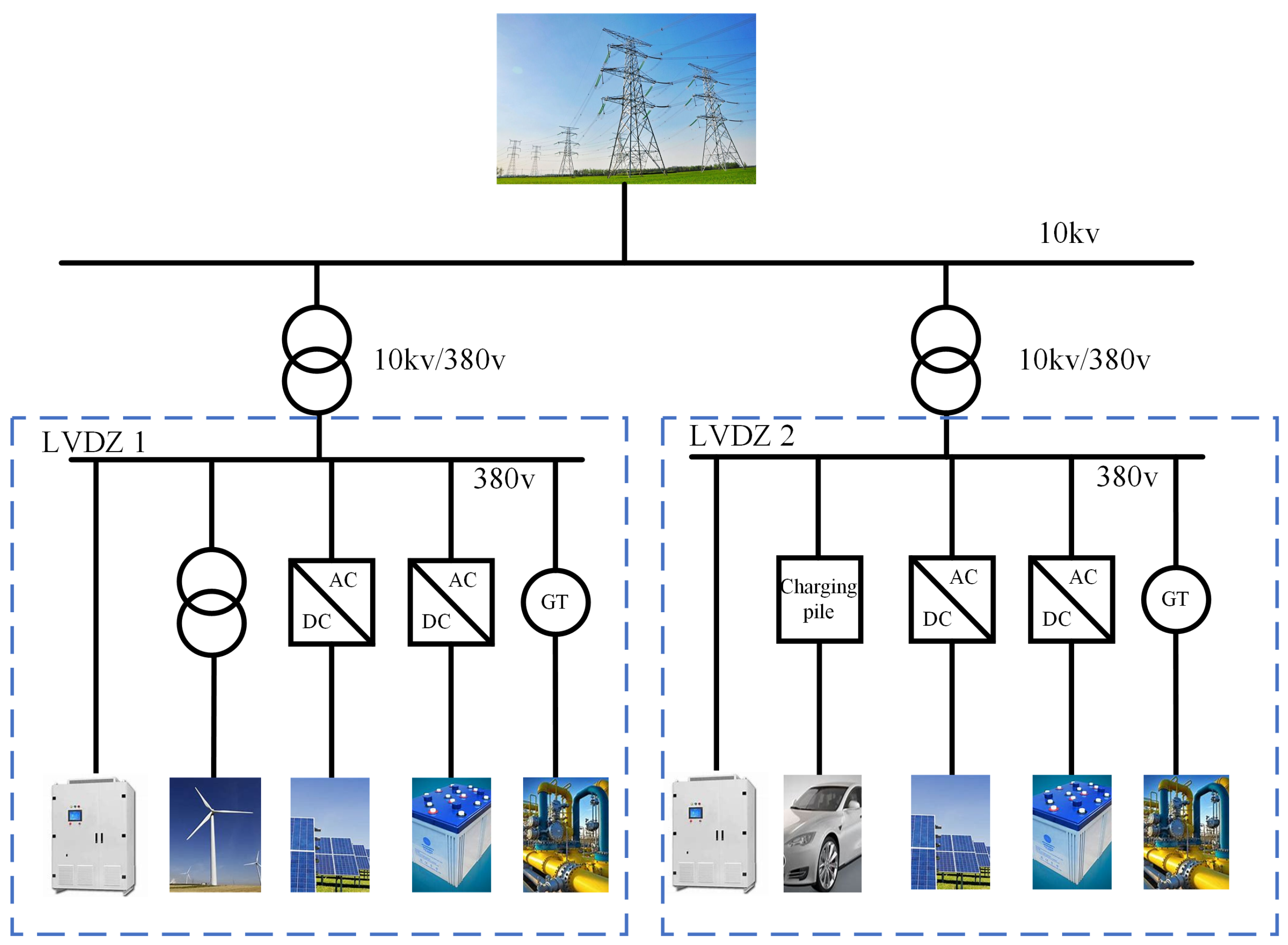
The operating point is the specific set of values corresponding to the operating parameters of each electrical component of a power system in a particular operating state. It represents the safety of the system in a particular state [18]. In a low-voltage distribution substation systems, loads represent energy demands. The power supply acts as the supply side and is responsible for meeting these demands. In this way, the system can guarantee safe operation. The operating point of the system is defined by key variables such as load, which are the basis for assessing the safety of the system. The structure of a low-voltage distribution substation station is shown in Figure 1. There are several types of energy sources included in modern bench systems, for example, wind energy, photovoltaic energy, natural gas, and energy storage.

There are two types of energy sources in the station: electricity and natural gas. In this paper, the liaison between the two is established through coupled units: the natural gas compressor serves as an electrical load, which is supplied with driving power by the electrical system part, and the gas turbine (GT) serves as a natural gas load, which receives the input flow from the natural gas network [19]. Therefore, in this paper, the operating point is denoted as

$$W=\left[S_{1,\mathrm{e}1}\dots S_{1,\mathrm{e}i},\dots S_{1,c1},\dots S_{1,cm},\dots ,G_{1,g1},\dots G_{1,gj},\dots ,G_{1,GT1},\dots G_{1,GTn}\dots \right]$$

(1)

where $S_{1,ei}$ is the nodal power of the power type load; $G_{1,gi}$ is the flow rate of natural gas; i, j is the number of nodes; $S_{1,ci}$ is the power consumed by the compressor; $G_{1,GTj}$ is the flow rate of natural gas consumed by the gas generator at node j.

2.2. Definition of Security

The LVDS studied in this paper can be considered part of an integrated energy system. Therefore, we define the safety of the low-voltage distribution substation (LVDS) as follows: the system is considered to be safe under a particular work point if all state quantities at that work point meet the constraints of operation. Such a work point is called a safe work point and is symbolized by $W_s$. On the contrary, if there exists any state quantity that does not satisfy the operational constraints, the work point is considered unsafe. In short, whether a work point is safe or not depends on whether all of its state quantities meet the established operational constraints.

2.3. Definition of Security Region

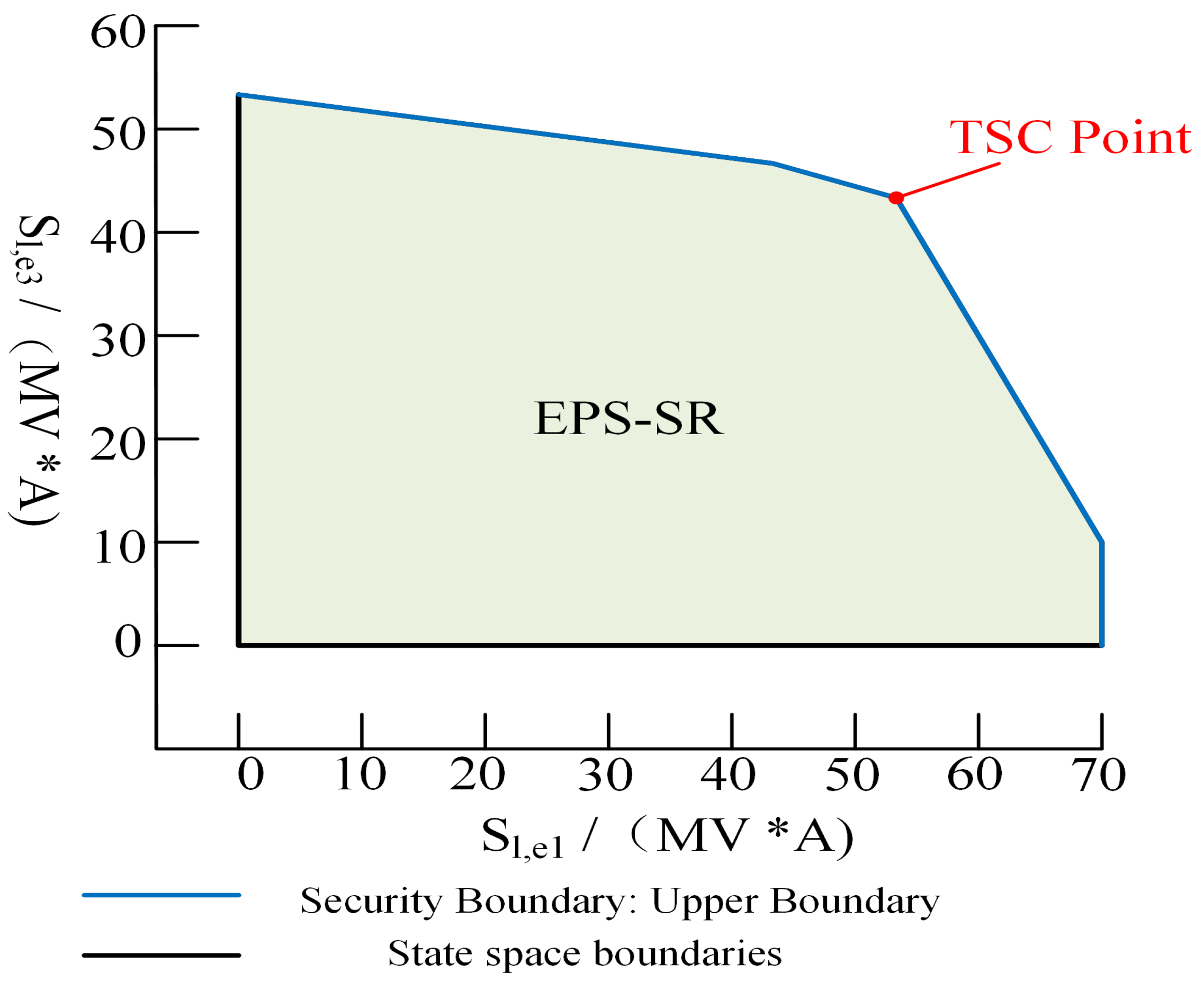
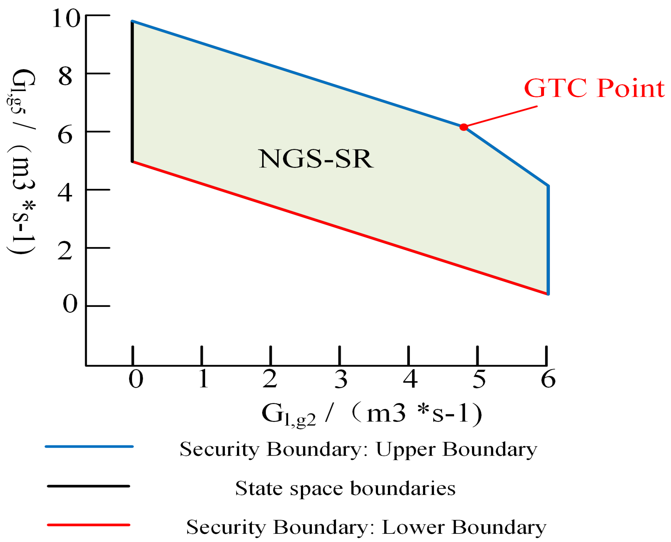
LVDS-SR is defined as the set of all safe operating points during LVDS running, denoted by ${\mathrm{\Omega }}_{LVDZ}$. The LVDS-SR is a closed region in the state space and consists of the EPS-SR and the NGS-SR. The safe boundary of the LVDS is defined as the set consisting of all critical points in the LVDS-SR, denoted by ${\delta }_{LVDZ}$. In this paper, total supply capability (TSC) and gas transmission capability (GTC) are used to measure the maximum supply potential of the LVDS during safe operation. The TSC and GTC points correspond to the operating states when the LVDS power supply and gas delivery are maximized, and they are the efficient working points in the LVDS-SR. Whether the work points are located in the safety domain is the key criterion to judge their safety. If the work point is located within the security domain, then the system is in a safe operating state. Conversely, if the work point is not within the security domain, then the system is at a security risk.

The specific location of work points within the safety domain also indicates the amount of safety margin. Using the security domain, grid operators can visually assess the current level of security of the system, clearly identifying how much system security margin is available in all directions, which enables them to make quick and accurate decisions about preventive measures or responses to emergencies. With this intuitive display of security status, dispatchers can manage the grid more effectively to ensure the reliability and security of the power supply.

3. Mathematical Modeling of LVDS

3.1. Energy Path Model

In heterogeneous energy modeling, energy circuit analysis is used to describe the energy flow process. Specifically, the flow of electrical energy is analyzed using electrical circuits, the flow of natural gas is analyzed using gas circuits, and the flow of thermal energy is analyzed using water and heat circuits [16]. Using the energy circuit model, mathematical models with the same mathematical form can be established to achieve a unified description of the energy flow equilibrium relationship of heterogeneous energy systems.

3.1.1. Mathematical Model of the Circuit Section

The circuit part is generally equated to the branch using a $\pi$-shaped circuit [20], which corresponds to the following mathematical model:

$$Y_{\mathrm{e}}{U}_{\mathrm{n}}=I_{\mathrm{n}}$$

(2)

where $Y_e$ is the nodal conductance matrix; $U_n$ and $I_n$ are the vectors consisting of the nodal voltage and injection current, respectively. The mathematical model of the circuit part can construct a unified energy path safety domain model, which is suitable for various network energy systems. The advantage of this approach is its generality, which facilitates extension and direct application to a wide range of power system analysis scenarios while fitting in with existing security domain research and modeling practices. This methodology has significant advantages. First, it is highly generalizable and easy to extend its application to a wide range of power system analysis scenarios. Second, it is consistent with existing security domain research and modeling practices. In addition, the mathematical model can be adapted to different types of tidal current analysis. In short, this approach provides a flexible framework that can be used to analyze many energy systems. It can ensure the safe operation of these systems under various conditions.

3.1.2. Mathematical Modeling of the Natural Gas Fraction

In the energy path model, the natural gas system is equated to the pipeline using a $\pi$-shaped gas path, and the $\pi$-shaped gas path parameters are calculated as follows at steady state:

$$Z_{\mathrm{b}}=2{\displaystyle \frac{R_{\mathrm{g}}}{k_{\mathrm{g}}}}sinh{\displaystyle \frac{k_{\mathrm{g}}l}{2}}{\mathrm{e}}^{-{\displaystyle \frac{k_{\mathrm{g}}l}{2}}}$$

(3)

$$k_{\mathrm{b}}=\left(cosh{\displaystyle \frac{k_{\mathrm{g}}l}{2}}-sinh{\displaystyle \frac{k_{\mathrm{g}}l}{2}}\right){\mathrm{e}}^{-{\displaystyle \frac{k_{\mathrm{g}}l}{2}}}$$

(4)

$$Y_1=0$$

(5)

$$Y_2=0$$

(6)

where $Z_b$ is the branch impedance of the $\pi$-shaped gas path, $k_b$ is the controlled gas pressure source, $Y_1$ and $Y_2$ pairs are the conductance to ground, and l is the tube length. $R_g$ and $k_g$ are the air distribution parameter gas resistance and controlled air pressure source, respectively, and are calculated as follows in steady state:

$$R_{\mathrm{g}}={\displaystyle \frac{\lambda {\nu }_{\mathrm{b}}}{sd}}$$

(7)

$$k_{\mathrm{g}}={\displaystyle \frac{2gdsin\theta -\lambda v_{\mathrm{b}}^2}{2RTs}}$$

(8)

where $v_b$, $\lambda$, s, d, and $\mathsf{\theta }$ are the friction coefficient, flow rate base value, cross-sectional area, internal diameter, and inclination of the pipeline, respectively; g is the gravitational acceleration; R and T are the natural gas constant and temperature, respectively. Ref. [21] derives the corresponding steady-state mathematical model for the gas circuit part, which is of the same form as the mathematical model for the electric power part:

$$Y_{\mathrm{g}}{p}_n=G_n$$

(9)

$p_n$ and $G_n$ are vectors composed of nodal natural gas pressure and flow, respectively; $Y_g$ is the generalized nodal conductivity matrix for the natural gas part.

3.2. Security Region Model

3.2.1. Security Regions

Using the energy path model, the steady-state model of LVDS-SR is of the form shown in Equation (10).

$${\mathrm{\Omega }}_{\mathrm{IES}}=\left\{W_s\mid h\left(W_s\right)=0,g\left(W_s\right)⩽0\right\}$$

(10)

where $W_s$ is the safe working point; $h\left(W_s\right)$ is the balance constraint; $g\left(W_s\right)$ is the safety constraint. The three types of constraints are shown in Equations (A1)–(A3) (see Appendix A).

It can be seen that the safety domain model of a single heterogeneous energy system is very easy to extend to the LVDS-SR model after the adoption of the energy path, the state quantities have a correspondence with each other, and their mathematical forms are harmonized with each other.

3.2.2. Security Boundary

The LVDS-SR security boundary model is shown in Equation (11). The meaning is as follows: $x_i$ is a work point element, $W_b\in {\mathrm{\Omega }}_{LVDS}$ means that the work point $W_b$ is located in the domain and is a safe work point, and a new work point $W^{*}$ is formed by adding ${\epsilon }^{*}$ to any element $x_i$ of $W_b$. If $\forall {\epsilon }^{*}\ne 0,\exists i=1,2,\cdots ,\mathrm{n}$, such that $W_b\in {\mathrm{\Omega }}_{LVDS}$, then $W_b$ is a boundary point, and all of Wb form a safe boundary. If ${\epsilon }^{*}>0$, then $W_b$ has positive criticality and lies on the upper boundary; if ${\epsilon }^{*}<0$, then $W_b$ lies on the lower boundary.

$$\left.{\partial }_{LVDZ}=\left\{W_{\mathrm{b}}\left|\begin{array}{c}[x_1,\cdots ,x_i,\cdots ,x_j,\cdots ,x_n]=W_{\mathrm{b}}\in {\mathrm{\Omega }}_{LVDZ}\\ W^{*}=[x_1^{*},\cdots ,x_i^{*},\cdots ,x_j^{*},\cdots ,x_n^{*}]\\ x_i^{*}=x_i+{\epsilon }^{*}\\ x_j^{*}=x_{j}j\ne i\\ \forall {\epsilon }^{*}\ne 0,\exists i=1,2,\cdots ,n,W^{*}\notin {\mathrm{\Omega }}_{LVDZ}\end{array}\right.\right.\right\}$$

(11)

4. Security Region Solving

4.1. Difficulties and Solution Ideas

The difficulty of solving the security domain increases with the high dimensionality of the LVDS work points since the LVDS-SR of the IES presents itself as a complex hyperpolyhedral shape in the high-dimensional state space. This leads to two main problems:

One is that it is difficult to directly observe and completely represent the security boundary of the LVDS-SR in high-dimensional space, and in particular, it is difficult to determine the cutoff point of the boundary curvature change, which is crucial for the accurate fitting of the boundary.

Secondly, with an increase in the dimension of the security domain, the number of work points to be verified increases dramatically, and it will be extremely time-consuming to continue to use the traditional multi-energy flow computation method to verify the security of each work point.

In this paper, the solutions to the above difficulties are as follows:

(1)

Difficulty 1: This paper proposes a method for fitting security boundary expressions applicable to high-dimensional state-space security domains. The method can automate the determination of the partition point by measuring the distance between the boundary point and the hyperplane. In addition, the fitting method does not need to obtain the partition where the security boundary undergoes curvature change by observation.

(2)

Difficulty 2: In this paper, a mathematical model is used to compute multiple energy flows instead of the complex energy flow equations in heterogeneous energy systems. This approach saves computational resources by reducing the need for repeated iterative solving of nonlinear equations.

4.2. Specific Steps of the Solution Method

Based on the above method, we obtain complete security domain results for high-dimensional LVDS-SRs. These results include security boundary points and security boundary expressions obtained by fitting. The specific process is as follows: firstly, mathematical model solving is carried out to obtain the complete state quantities of the working points, which is the basis of boundary point solving; secondly, boundary point solving is carried out to find the working points that satisfy the critical security; finally, the security boundary expression is obtained through the fitting of the security boundary.

4.2.1. Mathematical Model Solution

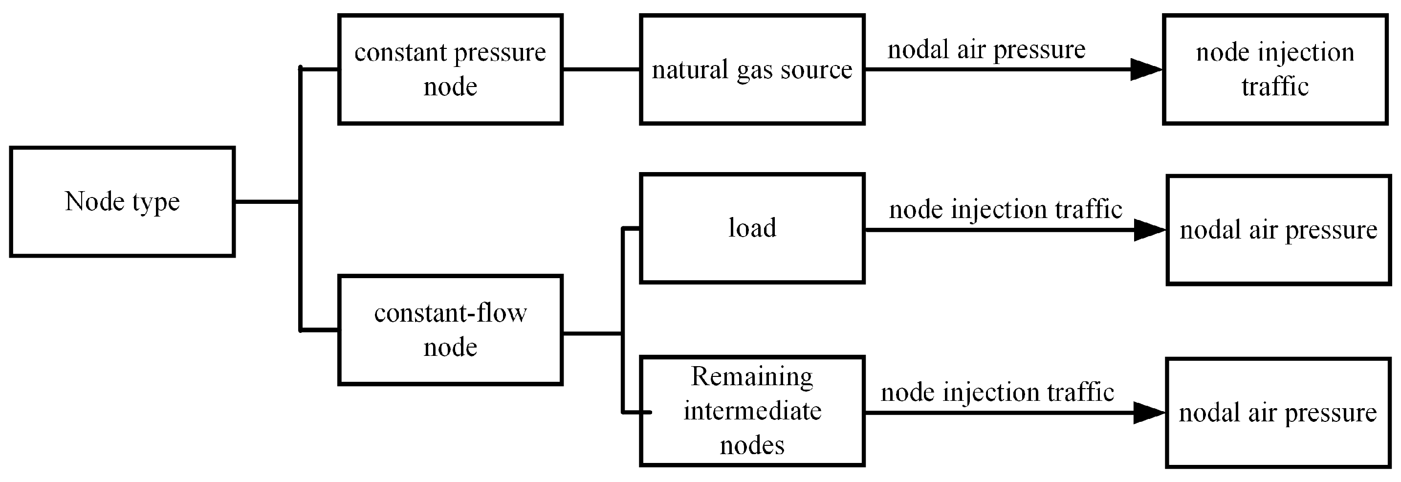
The nodes of the natural gas part can be divided into constant-pressure nodes and constant-flow nodes, as shown in Figure 2. Next, the mathematical model of Equation (9) is rearranged by node type to obtain

$$\left[\begin{array}{cc}{Y}_{g.pp}& Y_{g.pg}\\ Y_{g.gp}& Y_{g.gg}\end{array}\right]\left[\begin{array}{c}{p}_p\\ p_g\end{array}\right]=\left[\begin{array}{c}{G}_p\\ G_g\end{array}\right]$$

(12)

where $p_p$ is the nodal air pressure at a constant-pressure node and $G_p$ is the injected flow rate. $p_g$ is the nodal air pressure at a constant-flow node and $G_g$ is the injected flow rate. $Y_{g,pp}$, $Y_{g,pg}$, $Y_{g,gp}$ and $Y_{g,gg}$ are obtained by rearranging the generalized nodal conductivity matrix $Y_g$ for natural gas systems. The purpose of this rearrangement is to divide the matrix into different sub-matrices based on the type of nodes.

Finally, $G_p$ and $p_g$ can be solved from Equation (12) as follows:

$$G_{\mathfrak{p}}=Y_{\mathfrak{g},\mathfrak{p}\mathfrak{p}}{p}_{\mathfrak{p}}+Y_{\mathfrak{g},\mathfrak{p}\mathfrak{g}}{p}_{\mathfrak{g}}$$

(13)

$$p_{\mathrm{g}}=Y_{\mathrm{g},\mathrm{pg}}^{-1}(G_{\mathrm{g}}-Y_{\mathrm{g},\mathrm{gp}}{p}_{\mathrm{p}})$$

(14)

Mathematical model of the coupling part.

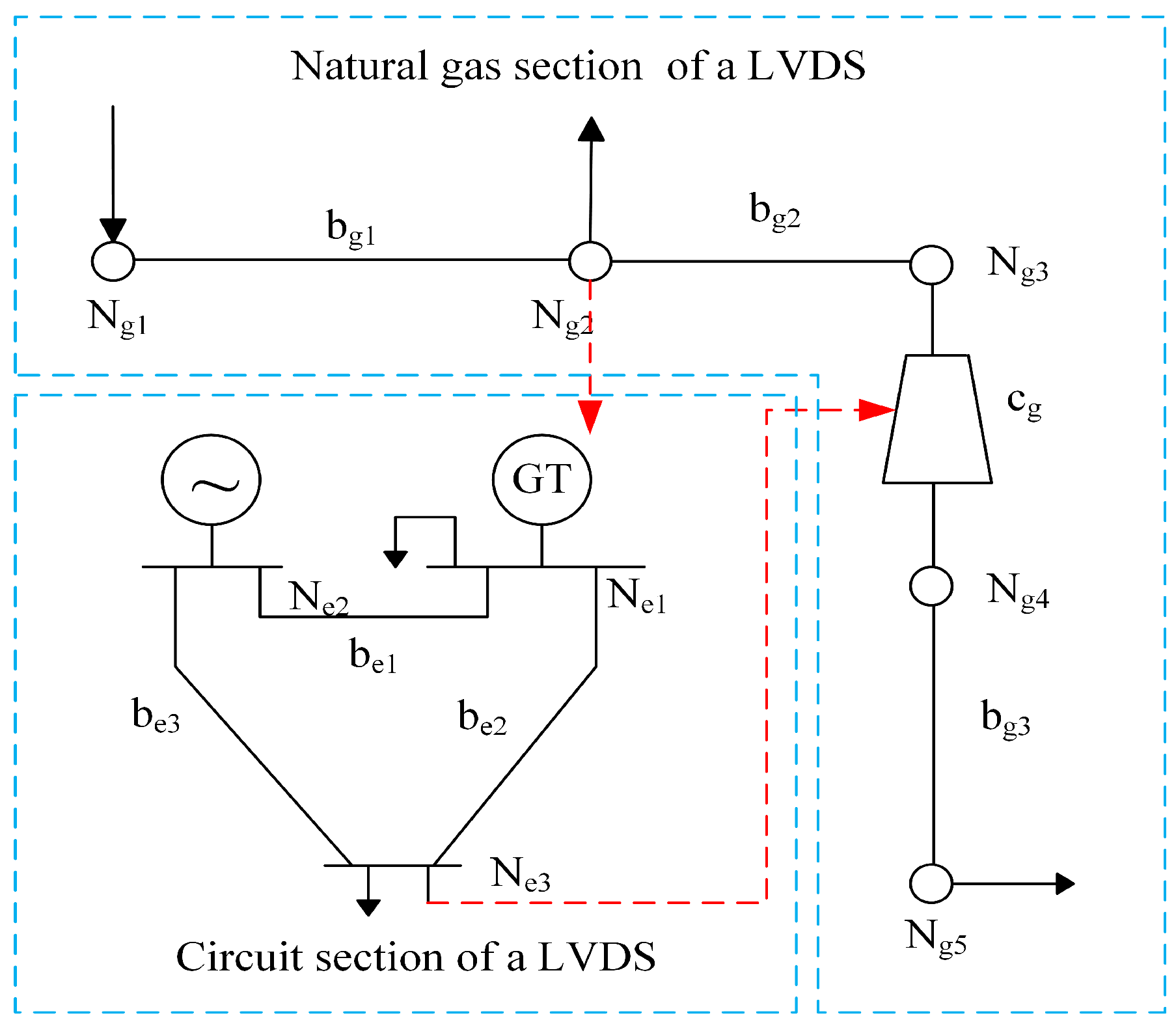
First, based on the energy flow relationship, the nodes where the coupling units in the LVDS are located are categorized as shown in Figure 3.

Subsequently, the natural gas mathematical model is solved based on the node division of the coupling unit in the natural gas network in order to obtain detailed state information on the natural gas system.

Finally, based on the coupled unit constraint equations in (14), the required state quantities of the coupled unit are calculated to solve the power system mathematical model, thus realizing the transfer of energy parameters between different energy systems.

4.2.2. Boundary Point Solving

There is a gas-path-based NGS-SR solving method proposed in [4], which uses the bisection method to solve for the boundary points by iteratively correcting the working points to the boundary points. In this paper, the method is used to solve LVDS-SR boundary points. When solving, any element of the working point is selected for correction, and the rest of the elements are sampled at equal intervals; at the same time, in order to facilitate the subsequent fitting of the security boundary, it is necessary to ensure that the number of boundary points obtained is not less than the number of security domain dimensions.

4.2.3. Safety Boundary Fitting

The LVDS-SR is a closed region in N-dimensional state space. When N > 3, the reduced-dimensional view of the domain and the corresponding boundary expression are often obtained by 2D/3D observation, but the reduced dimensionality can only reflect the local information of the LVDS-SR. The boundary points are N-dimensional, reflecting the LVDS-SR’s global information, but the boundary points are discrete in the state space, and the relative expressions are not easy to use. For this reason, this paper proposes a fitting method that can solve the security boundary expression of a high-dimensional LVDS-SR.

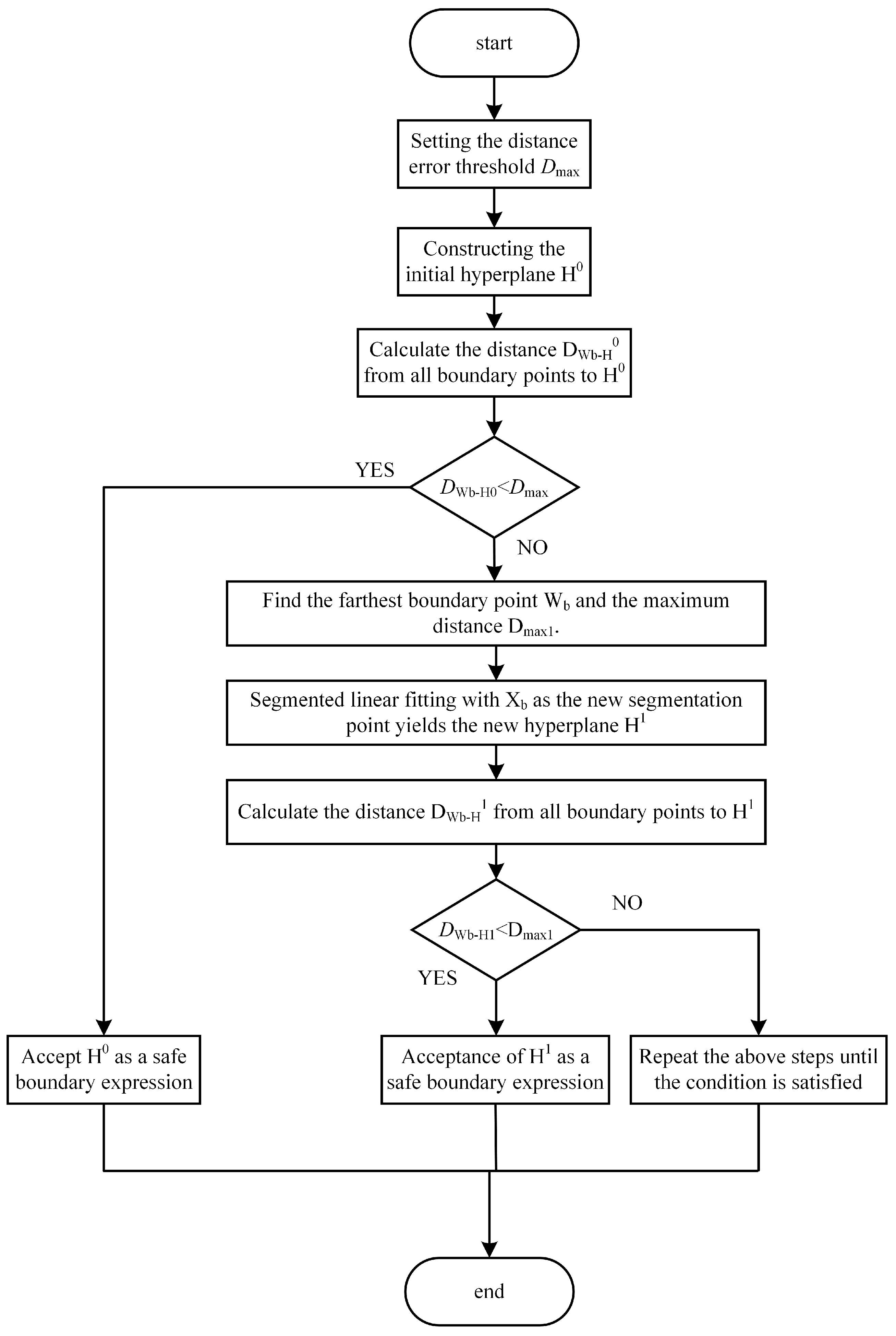
Analogous to the power system [22], a set of hyperplanes are used to inscribe the security boundary of the LVDS-SR, and a segmented linearization method is used to fit the hyperplanes. It is difficult to find suitable segment points between hyperplanes in high-dimensional space. This is because it is difficult to directly observe the segmentation where the boundary undergoes a large curvature change in the high-dimensional space. It calculates the distance from the boundary points to the hyperplane to achieve the automatic solution of the segmentation points. The program algorithm is specified in Figure 4:

The specific fitting steps are as follows:

(1)

Set the threshold of distance error $D^{max}$. $D^{max}$ represents the upper limit of the distance from all boundary points to the fitted hyperplane during the fitting process. It represents the fitting accuracy of hyperplanes and the end conditions of piecewise fitting.

(2)

Construct the initial hyperplane. First, in order to improve the fitting efficiency, the number of fitting iterations should be minimized on the basis of ensuring accuracy. Therefore, for the initial hyperplane fitted for the first time, N linearly irrelevant boundary points with the largest possible coverage domain range are selected for fitting. The initial hyperplane equations are as follows:

$$H^0:\sum _{i=1}^N{a}_i^0{\beta }_i+b^0=0$$

(15)

where $H^0$ is the initial hyperplane equation; $a_0^i$, $b_0$ are the fitting coefficients of $H^0$, which can be calculated from the boundary points selected in the fitting; ${\beta }_i$ is the variable of $H^0$ corresponding to the work point element; and N is the dimension of the LVDS-SR.

Next, the distance from each boundary point to $H^0$ is calculated. For the boundary point ${\mathrm{W}}_{\mathrm{b}}=[{\mathrm{x}}_1,\cdots ,{\mathrm{x}}_{\mathrm{i}},\cdots ,{\mathrm{x}}_{\mathrm{N}}]$, the distance ${\mathrm{D}}_{\mathrm{Wb}\to \mathrm{H}0}$ from $W_b$ to $H^0$ is

$$D_{W_{\mathrm{b}}\to H^0}={\displaystyle \frac{\left|{\sum }_{i=1}^N{a}_i^0{x}_i+b^0\right|}{{∥a_i^0∥}_2}}$$

(16)

where ${\mathbf{a}}_{\mathbf{0}}^{\mathbf{i}}$ is the vector of $a_0^i$; $\Vert a_i^0{\Vert }_2$ is the 2-parameter of $a_0^i$. Finally, record the boundary point $W_{\mathrm{b}}^{\left(0\right)}$ with the farthest distance to $H^0$ among all boundary points; the corresponding distance is recorded as $D_{w_b\to H^0}^{max}$, and judge whether $H^0$ satisfies the fitting accuracy: if $D_{W_{\mathrm{b}}\to H^0}^{max}⩽D^{max}$, then the accuracy is satisfied, and $H^0$ is the final boundary expression; otherwise, take $W_{\mathrm{b}}^{\left(0\right)}$ as a segmentation point, and group the boundary points selected when fitting $H^0$ for segmentation fitting.

(3)

Segmented linear fitting. The steps in the kth segmented fitting are as follows. First, for the selected boundary points, if the linear irrelevance condition is satisfied, hyperplanes of the form shown in (15) are fitted into hyperplanes by grouping, and a total of M hyperplane equations are obtained.

Next, the distance from the boundary point Wb to each hyperplane is calculated according to (16), and the smallest value is taken:

$$D_{W_{\mathrm{b}}\to H^k}=min\left(D_{W_{\mathrm{b}}\to H_j^k}\right)j=1,2,\cdots ,M$$

(17)

where $D_{W_b\to H^k}$ is the minimum distance from $W_b$ to all hyperplanes; $D_{W_b\to H_j^k}$ is the distance from $W_b$ to hyperplane $H_j^k$.

Finally, calculate $D_{W_b\to H^k}$ of all boundary points, take the maximum value of it, denoted as $D_{W_{\mathrm{b}}\to H^k}^{\max }$, and the corresponding boundary point is denoted as $W_{\mathrm{b}}^{\left(k\right)}$. Judge whether the kth segmented fitting meets the fitting accuracy: if $D_{W_k\to H^k}^{\max }⩽D^{\max }$, then it meets the accuracy, and all the distances from the boundary points to the hyperplane are within the error range, so that we can obtain the final safety boundary, and the safety boundary-fitting process is ended; otherwise, take $W_{\mathrm{b}}^{\left(k\right)}$ as the segmentation point, group the boundary points selected in the kth segmentation fitting, obtain N new hyperplanes, and continue the k+1th segmentation fitting. It should be noted that for the N-dimensional security domain, the uniqueness of the hyperplane fitting result is guaranteed by the fact that N linearly independent boundary points are selected for each of its hyperplane fittings.

5. Case Analysis

5.1. Raw Data of Test Cases

We use example 1 shown in Figure 5 as the test case for verification. The system consists of a 5-node natural gas system [4] and a 3-node electric power system [10]. In the figure, the power node $N_{e3}$ provides the electric power required to drive the compressor $c_g$, and the natural gas node $N_{g2}$ provides the natural gas power required by the gas turbine generator (GT). The specific parameters are shown in

Table 1. Natural gas system node parameters.

Nodal	Actual Node Type	ir Pressure Range/MPa	Flow Range/(${\mathbf{m}}^3·{\mathbf{s}}^{-1}$)
$N_{g1}$	Gas distribution node	[4.5, 6.0]	(−∞, 0]
$N_{g2}$, $N_{g5}$	Load node	[2, 5]	[0, 10]
$N_{g3}$	Compressor inlet node
$N_{g4}$	Compressor discharge node

Note: The pressure ratio range of the compressor is [1, 2].

,

Table 2. Natural gas system pipeline parameters.

Plumbing	Beginning	End Point	Pipe Diameter/m	Length/km	Capacity/(${\mathbf{m}}^3·{\mathbf{s}}^{-1}$)
$b_{g1}$	$N_{g1}$	$N_{g2}$	0.20	70	15
$b_{g2}$	$N_{g2}$	$N_{g3}$	0.20	25	15
$b_{g3}$	$N_{g5}$	$N_{g5}$	0.20	25	15

,

Table 3. Power system branch circuit parameters.

Branch Road	Beginning	End Point	Resistance/p.u.	Reactance/p.u	Dena/p.u	Capacity/(MV·A)
$b_{e1}$	$N_{e1}$	$N_{e2}$	0.04	0.5	0	55
$b_{e2}$	$N_{e2}$	$N_{e3}$	0.04	0.5	0	55
$b_{e3}$	$N_{e3}$	$N_{e3}$	0.04	0.3	0	55

and

Table 4. Power system node parameters.

Nodal	Node Type	Voltage Amplitude Range/p.u.	Voltage Amplitude Range/p.u.	Generator Reactive Power Range/(Mvar)	Load Apparent Power Range/(MV·A)	Load Power Factor
$N_{e1}$	PV node	[0.90, 1.00]	[0, 55]	[−55, 55]	[0, 80]	0.95
$N_{e2}$	balancing node	1	[0, 110]	[−110, 110]
$N_{e3}$	PQ node	[0.90, 1.10]			[0, 80]	0.95

Note: The voltage is standardized with a reference value of 110 kV.

.

5.2. Test Case Security Domain Solving and Observation

Its solution contains the expression of the boundary points and the safety boundary obtained by the LVDS-SR method. The result is a view with a reduced local dimension. The experimental configuration is as follows: the processor used is a 2.5 GHz Intel Core i7 8th generation equipped with 8 GB of RAM, and the simulation platform is IntelliJ IDEA.

5.2.1. Complete Solution Results for the Security Domain

The solution parameters are as follows: load power at node 1 ($S_{1,e1}$), load power at node 3 ($S_{1,e3}$) in the power system, electric power consumed by the natural gas compressor ($S_{1,c}$), the flow rate at node 2 in the natural gas system ($S_{1,g2}$), and gas flow rate consumed by gas turbine (GT) ($S_{1,GT}$). By sampling at equal intervals in the state space, correcting $G_{1,g5}$, and correcting the convergence accuracy of 0.01, a total of 25,735 points of the upper boundaries are obtained, as shown in

Table 5. LVDS-SR upper-boundary points for Calculation 1.

Border Point	Work Point	Total Power Supply/(MV·A)	Volume/(${\mathbf{m}}^3·{\mathbf{s}}^{-1}$)
$W_{b,1}$	(5, 5, 0.65, 1, 3, 9.88)	9.55	14.80
$W_{b,2}$	(5, 5, 0.65, 1, 5, 9)	9.55	14.00
…	…	…	…
$W_{b,25735}$	(70, 15, 1.58, 1, 8, 4.80)	84.7	15.20

, and 12,118 points of the lower boundaries, as shown in

Table 6. LVDS-SR lower-boundary points for Calculation 1.

Border Point	Work Point	Total Power Supply (MV·A)	Total Gas Volume (${\mathbf{m}}^3·{\mathbf{s}}^{-1}$)
$W_{b,1}$	(65.5, 15, 2.74, 1, 8, 4.63)	84.27	14.53
$W_{b,2}$	(65.5, 15, 2.53, 1, 8, 4.25)	85.88	14.44
…	…	…	…
$W_{b,12115}$	(7.5, 7.5, 0, 1, 0, 6.62)	15.00	7.49

.

We calculate the total power supply and total gas transmission at the boundary points. The TSC value of example 1 is 97.83 MV·A and the GTC value is 14.94 ${\mathrm{m}}^3·$  ${\mathrm{s}}^{-1}$.

Table 7. TSC and GTC points for Calculation 1.

Typology	Work Point	Total Power Supply (MV·A)	Total Gas Volume (${\mathbf{m}}^3·{\mathbf{s}}^{-1}$)
TSC Point	(54.5, 41.5, 2.77, 1, 8, 4.87)	96.73	14.92
GTC points	(25.5, 34.5, 1.58, 5, 4, 5.87)	72.44	14.92
	…	…	…
	(75, 5, 0.65, 1, 9, 4.88)	81.45	14.92

shows the corresponding TSC points and GTC points, which represent the operating state of the LVDS at its maximum power supply and gas transmission. These points are the high-efficiency operating points in the LVDS-SR, which represent the operating state when the LVDS power supply and gas transmission capacity are maximized, respectively.

Using the boundary points to fit the security boundary and setting the distance error threshold at 0.1, 45 upper-boundary hyperplanes and 65 lower-boundary hyperplanes can be obtained, as shown in

Table 8. Security boundary expressions for Calculation 1.

Security Border	Hyperplane	Displayed Formula
Upper Boundary	1	−9904 $S_{1,e3}$ + 49,532 = 0
(45 hyperplanes in total)	2	−1152 $S_{1,e1}$ + 32,758 $S_{1,c}$ + 279,735 $G_{1,g2}$ + 280,745 $G_{1,g5}$ + 355,258 $G_{1,g5}$ − 5,564,860 = 0
	3	−62,024 $G_{1,g2}$ + 62,024 = 0
	…	…
	44	−1220 $S_{1,e1}$− 498 $S_{1,e3}$ + 33,795 $S_{1,c}$ − 247,699 $G_{1,g2}$ − 247,699 $G_{1,GT}$ − 268,045 $G_{1,g5}$ + 4,681,577 = 0
	45	−1388 $S_{1,e1}$− 178 $S_{1,e3}$ + 40,034 $S_{1,c}$ − 276,034 $G_{1,g2}$ − 305,977 $G_{1,GT}$ − 304,485 $G_{1,g5}$ + 3,949,485 = 0
Lower Boundary	1	735 $S_{1,e1}$ − 19,225 $S_{1,e3}$ − 780,031 $S_{1,c}$ + 198,825 $G_{1,g2}$ + 285,287 $G_{1,GT}$ + 427,685 $G_{1,g5}$ − 1,697,325 = 0
(65 hyperplanes in total)	2	−17754 $S_{1,e1}$ + 1674 $S_{1,e3}$ − 365,035 $S_{1,c}$ + 207,834 $G_{1,g2}$ + 161,655 $G_{1,GT}$ + 354,358 $G_{1,g5}$ − 1,688,726 = 0
	3	−3045 $S_{1,e1}$ + 23,874 $S_{1,e3}$ + 533,253 $S_{1,c}$ − 347,761 $G_{1,g2}$ − 305,567 $G_{1,GT}$ − 456,560 $G_{1,g5}$ + 4,076,718 = 0
	…	…
	64	345 $S_{1,e1}$ + 2165 $S_{1,e3}$ − 30,056 $S_{1,c}$ + 32,578 $G_{1,g2}$ + 29,430 $G_{1,GT}$ + 27,490 $G_{1,g5}$ − 4,535,894 = 0
	65	−12,728 $S_{1,e1}$− 1785 $S_{1,e3}$ − 866,589 $S_{1,c}$ + 467,546 $G_{1,g2}$ + 346,927 $G_{1,GT}$ + 574,485 $G_{1,g5}$ − 3,345,267 = 0

.

5.2.2. Localized Observations of the Security Domain

The local 2D view of LVDS-SR is observed. Meanwhile, in order to observe the geometrical relationship between the TSC and GTC points and the domain, this paper is based on the observation of the load distribution under the TSC and GTC points.

Figure 6 shows the results when $N_{e1}$, and $N_{e3}$ are observation nodes based on TSC points (55, 40, 2.83, 1, 9, 4.94). Since the observation nodes are power nodes, this view mainly visualizes the partial results of the EPS-SR in the LVDS-SR. It can be seen that this part of the domain is enclosed by the upper boundary and the state space boundary, and the TSC points are located at the upper boundary.

Figure 7 shows the results when $N_{g}2$ and $N_{g}5$ are observation nodes based on GTC points (25, 35, 1.54, 5, 4, 5.94). Since the observation nodes are natural gas nodes, this view mainly visualizes the partial results of the NGS-SR in the LVDS-SR. It can be seen that this part of the domain is surrounded by the upper, lower, and state-space boundaries, and the GTC points are also located at the upper boundary.

It should be noted that all the LVDS-SRs observed in this paper are convex sets, which is consistent with mainstream research results. The reason that the security domain is a convex set is that the load injection power is selected as the working point element in this paper.

5.3. Comparison with Existing Methods

First of all, we have shown that existing methods still cannot solve difficulty 1 mentioned in Section 4.1. The existing [10] is only for the two-dimensional and three-dimensional cases, and the complete analytical formula of the high-dimensional security boundary has not been obtained. In this paper, the complete boundary analytic formula of the security boundary of the high-dimensional low-voltage distribution substation area security domain is obtained for the first time, which has the following advantages:

(1)

The complete safety boundary expression contains the global information of the safety domain of the LV substation area, which portrays the complete boundary of the safe operation of the LV substation area in the high-dimensional state space, while the existing methods can only obtain the downscaled result of the safety region of the LV substation area in the high-dimensional space, which only contains the local information of the safety domain of the LV substation area, and only portrays part of the boundary of the safe operation of the LV substation area.

(2)

The safety boundary expression can be used to analyze the safety of any work point in the state space and calculate the safety margin of the work point in all directions in the state space [23], while the existing methods can only analyze the safety of the work point located in the reduced-dimensional section, and can only calculate the safety margin in the direction of the section dimension [21].

Secondly, regarding the difficulty of solving the safety domain of the low-voltage transformer substation in Section 3.1, we compare the accuracy and time consumption of solving the boundary points of the safety domain of the low-voltage transformer substation between the existing methods and the method in this paper. Ref. [10] first proposed the concept of the low-voltage distribution substation safety domain using heterogeneous energy system inherent energy flow equation modeling; subsequent studies were performed in [10] on the basis of the expansion of the basic model and [10], but no essential difference was found between that and [23]. Therefore, this paper selects the method of [10] for comparison. The comparison results are shown in

Table 9. First comparison of the accuracy and time consumption for solving the boundary points between this method and the existing methods.

Type of Work Point	Solution Results	Solving Time (ms)
Upper-boundary points (29,695)	(4, 4, 0.43, 1, 2, 8.683489)	7.18
	(4, 4, 0.43, 1, 3, 8.502833)	6.01
	(4, 4, 0.43, 1, 5, 7.235622)	4.45
	…	…
	(85, 15, 1.76, 1, 9, 3.876147)	3.35
Lower-boundary points (15,105)	(58.5, 10, 2.77, 1, 9, 4.563452)	7.02
	…	…
	(58.5, 10, 0.59, 1, 9, 0.301971)	3.43
	…	…
	(5.5, 5.5, 0, 1, 0, 6.593848)	3.71
Total		174.342

and

Table 10. Second comparison of the accuracy and time consumption for solving the boundary points between this method and the existing methods.

Solution Results	Solving Time (ms)	Solving Result Relative Deviation (%)
(4, 4, 0.43, 1, 2, 8.683478)	0.52	$7.93\times {10}^{-5}$
(4, 4, 0.43, 1, 3, 8.502827)	0.39	$9.01\times {10}^{-5}$
(4, 4, 0.43, 1, 5, 7.235616)	0.31	$8.52\times {10}^{-5}$
…	…	…
(85, 15, 1.76, 1, 9, 3.876136)	0.29	$2.33\times {10}^{-4}$
(58.5, 10, 2.77, 1, 9, 4.563448)	0.42	$1.15\times {10}^{-4}$
…	…	…
(58.5, 10, 0.59, 1, 9, 0.301968)	0.32	$1.44\times {10}^{-3}$
…	…	…
(5.5, 5.5, 0, 1, 0, 6.593848)	0.29	$1.22\times {10}^{-4}$
	6.88

.

The following can be seen from Table 9 and Table 10:

(1) The number of boundary points obtained by the two methods is the same, and the boundary points correspond to each other.

(2) The deviation of the boundary points obtained by the two methods is very small, and the maximum relative deviation is only 0.00144%. This deviation does not affect the conservatism of the solution results because it only affects the accuracy of the boundary points after 0.00001, which is much smaller than the convergence accuracy of 0.01 set in the correction of the boundary points. The reasons for the small deviation are as follows:

Existing methods model heterogeneous energy systems using their inherent energy flow equations, which are more accurate. In this paper, errors are introduced when heterogeneous energy systems are modeled uniformly. The error is mainly due to the introduction of the base value of the pipeline flow rate in the gas path: if the base value is equal to the actual natural gas flow rate, the network equations in this paper are equivalent to the pipeline pressure drop equations, and theoretically, there will be no error. Reasonable determination of the base value can effectively reduce the error [24].

Table 9 and Table 10 also show that the efficiency of solving boundary points in this paper is greatly improved: the existing method takes 174.342 s to solve all boundary points, and the method in this paper takes a total time of 6.88 s, which is 25.48 times more efficient. It should be noted that the efficiency improvement is due to the linearization, as follows: when carrying out the unified modeling of heterogeneous energy sources, the momentum conservation equation of the flow process is linearized by using the network equations instead of the inherent energy flow equations of the heterogeneous energy network [25], which avoids the iterative process of solving the pressure drop equation of the pipeline in the calculation of the multi-energy flow, and saves computation time.

It should be noted that, due to the small deviation of the boundary points obtained by this paper’s method and the existing methods, the safe boundary expressions obtained by fitting using the two sets of boundary points are the same, and both are shown in the results of Table 8. This result further validates the correctness of the method in this paper.

6. Discussion

1.

This paper proposes a method for modeling the safety domain of low-voltage distribution substations based on the definition of high-dimensional safety domains, and it obtains the complete analytical expression of high-dimensional safety domains for the first time. Compared with existing research, it is evident that the method proposed in this paper has significant advantages. In the high-dimensional space, the method in this paper can automatically fit the safety boundary. This feature solves the problem that traditional methods have difficulty directly observing and completely representing the high-dimensional security boundary. Therefore, the method in this paper provides a new tool for the security analysis of power systems.

2.

In this paper, it is assumed that the safe operation range of low-voltage distribution substations can be described more accurately by high-dimensional safety region modeling. At the same time, this method can improve the solving efficiency. The research results show that the hypothesis is verified. By accurately solving the safety domain model, the safety boundary of the substation system can be clearly demonstrated and comprehensive safety assessment information can be provided to the dispatchers. In addition, the linearization method significantly reduces the time consumption for solving the boundary points, which provides the possibility of real-time safety analysis.

3.

The research results of this paper are theoretically significant. At the same time, they have important practical application value for the security assessment and optimization of power systems. The high-dimensional security domain model can visually assess the security level of the system. It can provide guidance for power grid planning and operation. At the meantime, the model can also optimize resource allocation, which in turn improves the reliability and stability of the system. In addition, this study provides new ideas for the security analysis of integrated energy systems, which helps to promote the theoretical development and practical application in related fields.

7. Conclusions

In this paper, a LVDS safety domain (LVDS-SR) modeling method based on the high-dimensional safety domain definition method is proposed for the problem of safety domain modeling of an LVDS in high-dimensional state space. The safety domain model of the LVDS is successfully constructed by solving the general mathematical model, edge points, and safety boundaries of the table system accurately. The main contributions and conclusions of this study are as follows:

(1)

The foundation of the theory and the introduction of concepts: This paper introduces the concepts of security operating points, security boundaries, and security domains. These concepts provide a solid theoretical basis for subsequent analysis and modeling. Through the clear definition of these core concepts, this study has laid a foundation for the analysis of the safety domain in the low-voltage transformer region.

(2)

Accurate solving and model construction: Through the high-dimensional safety domain definition-solving method, this study accurately solves the general mathematical model, edge points, and safety boundaries of the station area system, thus obtaining the safety domain model. This process not only improves the solving efficiency but also obtains the complete analytical formula of the high-dimensional security domain for the first time, which has important theoretical and practical application value for the security assessment and optimization of power systems.

(3)

Full boundary-fitting method: For the problem that it is difficult to directly observe the security boundary curvature change demarcation points in the high-dimensional space, this paper proposes an automated boundary point-fitting method, which realizes the automatic solution of the segmented points by measuring the distance between the boundary points and the hyperplane, and improves the fitting accuracy of the security boundary.

References

1. Zhong, Y.; Ji, L.; Wang, Z. Development Analysis and Discussion of Integrated Energy Service Under Dual-Carbon Target in China. In Proceedings of the 2023 International Conference on Power System Technology (PowerCon), Jinan, China, 21–22 September 2023; pp. 1–6. [Google Scholar] [CrossRef]
2. Batchu, S.; Teeparthi, K. Transient Stability Assessment and Enhancement in the Realm of Power System Dynamic Security Analysis: A Review and Scope of Methods. In Proceedings of the 2023 4th IEEE Global Conference for Advancement in Technology (GCAT), Bangalore, India, 6–8 October 2023; pp. 1–8. [Google Scholar] [CrossRef]
3. Tabebordbar, A.; Rastegar, M. Reliability Assessment of Integrated Electricity and Natural Gas Transmission Systems in Presence of Power-to-gas and Combined Heat and Power Technologies. CSEE J. Power Energy Syst. 2023, 9, 1193–1202. [Google Scholar] [CrossRef]
4. Zhang, X.; Liu, Y.; Han, Z.; Zhang, H. Enhancing Low-Voltage Distribution Network Safety through Advanced Residual Current Protection Techniques. Appl. Sci. 2024, 14, 3256. [Google Scholar] [CrossRef]
5. An, J.; Yu, J.; Li, Z.; Zhou, Y.; Mu, G. A Data-driven Method for Transient Stability Margin Prediction Based on Security Region. J. Mod. Power Syst. Clean Energy 2020, 8, 1060–1069. [Google Scholar] [CrossRef]
6. Savchenko, N.; Dovgalyuk, O.; Tretiak, A.; Syromyatnikova, T. Improving the Energy Efficiency of Small Hydropower Plants by Connecting an Energy Saving System with Kinetic Energy Storage. In Proceedings of the 2023 IEEE 5th International Conference on Modern Electrical and Energy System (MEES), Kremenchuk, Ukraine, 27–30 September 2023; pp. 1–6. [Google Scholar] [CrossRef]
7. Siface, D. Mathematical Modelling of Power-to-Gas Devices for the Medium Term Simulation of Integrated Energy Systems. In Proceedings of the 2020 AEIT International Annual Conference (AEIT), Catania, Italy, 23–25 September 2020; pp. 1–6. [Google Scholar] [CrossRef]
8. Ba, M.; Li, X.; Ru, Q.; Song, Z.; Zhang, Q.; Li, S. Optimal Dispatching Model of Integrated Energy System Considering Power to Gas and Carbon Capture System. In Proceedings of the 2022 3rd International Conference on Advanced Electrical and Energy Systems (AEES), Lanzhou, China, 23–25 September 2022; pp. 26–30. [Google Scholar] [CrossRef]
9. Chen, S.; Wei, Z.; Sun, G.; Wei, W.; Wang, D. Convex Hull Based Robust Security Region for Electricity-Gas Integrated Energy Systems. IEEE Trans. Power Syst. 2019, 34, 1740–1748. [Google Scholar] [CrossRef]
10. Su, J.; Chiang, H.D.; Alberto, L.F.C. Two-Time-Scale Approach to Characterize the Steady-State Security Region for the Electricity-Gas Integrated Energy System. IEEE Trans. Power Syst. 2021, 36, 5863–5873. [Google Scholar] [CrossRef]
11. Su, J.; Chiang, H.D.; Zeng, Y.; Zhou, N. Toward Complete Characterization of the Steady-State Security Region for the Electricity-Gas Integrated Energy System. IEEE Trans. Smart Grid 2021, 12, 3004–3015. [Google Scholar] [CrossRef]
12. Li, S.; Wang, D.; Zhu, Y.; Liu, L.; Jia, H. Multi-objective Optimal Control Based on Practical Security Region of Regional Integrated Energy System. In Proceedings of the 2020 IEEE Power & Energy Society General Meeting (PESGM), Montreal, QC, Canada, 2–6 August 2020; pp. 1–5. [Google Scholar] [CrossRef]
13. Liu, L.; Wang, D.; Hou, K.; Jia, H.j.; Li, S.y. Region model and application of regional integrated energy system security analysis. Appl. Energy 2020, 260, 114268. [Google Scholar] [CrossRef]
14. Liu, K.; Chen, H.; Li, S.; Wang, D.; He, G.; Zheng, H.; Liu, X.; Zhang, Y. Security and Energy Supply Valleys Assessment of Regional Integrated Energy System Based on Practical Security Region. In Proceedings of the 2021 IEEE 5th Conference on Energy Internet and Energy System Integration (EI2), Taiyuan, China, 22–24 October 2021; pp. 1474–1478. [Google Scholar] [CrossRef]
15. Jiang, T.; Zhang, R.; Li, X.; Chen, H.; Li, G. Integrated energy system security region: Concepts, methods, and implementations. Appl. Energy 2021, 283, 116124. [Google Scholar] [CrossRef]
16. Zhang, S.; Gu, W.; Zhang, X.P.; Lu, H.; Lu, S.; Ding, S.; Wang, J.; Zhao, S. Steady-State Security Region of Integrated Energy System Considering Thermal Dynamics. IEEE Trans. Power Syst. 2024, 39, 4138–4153. [Google Scholar] [CrossRef]
17. Chen, B.; Guo, Q.; Yin, G.; Wang, B.; Pan, Z.; Chen, Y.; Wu, W.; Sun, H. Energy-Circuit-Based Integrated Energy Management System: Theory, Implementation, and Application. Proc. IEEE 2022, 110, 1897–1926. [Google Scholar] [CrossRef]
18. Li, F.; Niu, T.; Xue, L.; Li, Y.; Huang, T.; Wu, Z. Autonomous-synergic Voltage Security Regions in Bulk Power Systems. J. Mod. Power Syst. Clean Energy 2023, 11, 686–692. [Google Scholar] [CrossRef]
19. Yan, C.; Bie, Z.; Liu, S.; Urgun, D.; Singh, C.; Xie, L. A Reliability Model for Integrated Energy System Considering Multi-energy Correlation. J. Mod. Power Syst. Clean Energy 2021, 9, 811–825. [Google Scholar] [CrossRef]
20. Xifan Wang, Y.S.; Irving, M. Modern Power Systems Analysis; Springer: Berlin/Heidelberg, Germany, 2008. [Google Scholar] [CrossRef]
21. Jun, X.; Baoqiang, Z.; Jingpeng, S.; Miaomiao, Z.; Guodong, Z. Full-dimensional Observation of Distribution System Security Region. Autom. Electr. Power Syst. 2018, 14, 2217–2226. [Google Scholar]
22. Liu, S.; Yin, X.; Zhao, Y.; Wang, D. Steady-State Modeling and Power Flow Calculation of Integrated Electric-Gas Coupling Energy System Based on Energy Circuit Theory. Commun. Comput. Inf. Sci. 2021, 8, 217–228. [Google Scholar]
23. Xiao, J.; Zhen, G.; Wang, B.; Wang, C. Security Distance of Distribution Network: Definition and Method. Zhongguo Dianji Gongcheng Xuebao/Proc. Chin. Soc. Electr. Eng. 2017, 37, 2840–2851. [Google Scholar]
24. Wu, Q.; Chen, M.; Ren, H.; Shi, S.; Su, Y.; Lu, J. Dynamic energy flow analysis of electricity-heating based integrated energy system. Energy Rep. 2023, 9, 193–205. [Google Scholar] [CrossRef]
25. Lee, M.; Park, J.; Na, S.I.; Choi, H.S.; Bu, B.S.; Kim, J. An Analysis of Battery Degradation in the Integrated Energy Storage System with Solar Photovoltaic Generation. Electronics 2020, 9, 701. [Google Scholar] [CrossRef]
26. Kanelakis, N.G.; Biskas, P.N.; Chatzigiannis, D.I.; Bakirtzis, A.G. A Stochastic Two-Stage Model for the Integrated Scheduling of the Electric and Natural Gas Systems. IEEE Open Access J. Power Energy 2020, 7, 453–466. [Google Scholar] [CrossRef]
Figure 1. Overall layout of low-voltage substation.
Energies 18 01153 g001
Figure 2. Classification of natural gas nodes.
Energies 18 01153 g002
Figure 3. Classification of coupled unit nodes.
Energies 18 01153 g003
Figure 4. Flowchart of the proposed algorithm.
Energies 18 01153 g004
Figure 5. Calculation example 1: system structure of the station.
Energies 18 01153 g005
Figure 6. Local observation view of LVDS-SR for Calculation 1 (observation nodes: N e 1 , N e 3 ).
Energies 18 01153 g006
Figure 7. Local observation view of LVDS-SR for Calculation 1 (observation nodes: N g 2 , N g 5 ).
Energies 18 01153 g007