

Bridging the Gap to Decarbonization: Evaluating Energy Renovation Performance and Compliance


Abstract
1. Introduction
1.1. Background and Importance
1.1.1. The Role of Energy Renovations
- Improving the building envelope performance, such as adding insulation, installing high-performance windows, and enhancing airtightness.
- Upgrading heating, ventilation, and air conditioning (HVAC) systems with more efficient and renewable-based technologies, including heat pumps, district heating, and waste heat recovery.
- Integrating renewable energy systems, including solar photovoltaic (PV) panels and battery storage.
- Enhancing smart energy management systems to optimize building operations and reduce peak loads.
1.1.2. Energy Performance Regulations and Their Impact
1.1.3. The Need for Accurate Energy Simulation Methods
- Fluctuating weather conditions and climate change projections.
- Occupancy behavior and operational variations.
- Thermal mass effects and heat retention properties of building materials.
- Renewable energy generation profiles, which vary hourly and seasonally.
1.2. Research Gap
1.3. Objectives
- Evaluate the accuracy of energy demand predictions by comparing static and dynamic simulation models across five renovation scenarios, identifying discrepancies and uncertainties in their projections.
- Assess the impact of simulation model selection on CO2 emissions reduction, determining whether static models overestimate energy savings and underestimate real-world energy consumption.
- Analyze the financial implications of simulation inaccuracies, investigating how misleading performance predictions may lead to over- or under-investment in energy retrofitting projects.
- Explore the potential of dynamic simulations in optimizing decarbonization pathways, providing evidence-based recommendations for integrating advanced modeling techniques into regulatory frameworks to enhance long-term energy efficiency and sustainability outcomes.
2. Methodology
2.1. Assessing the Thermal Envelope’s Performance in Renovated Buildings
2.2. Case Study Buildings and Renovation Models
- Building type and age: A mix of residential, commercial, and public buildings with varying construction dates to capture diverse renovation needs.
- Climate zone: Buildings are situated in different microclimates to assess the influence of climate conditions on energy performance.
- Renovation scope: Selected buildings encompass a wide range of energy efficiency measures, including insulation, HVAC upgrades, and renewable energy integration.
- Availability of energy performance data: Each building has accessible pre- and post-renovation data, allowing for a comparative analysis of energy efficiency improvements.
2.2.1. Building Classification and Renovation Strategies
- Building Envelope Upgrades: Thermal insulation improvements include upgrading walls, roofs, and floors with high-performance materials to reduce heat losses. Window and glazing replacement involve installing triple-glazed, low-emissivity windows to enhance thermal performance. Airtightness improvements focus on sealing thermal bridges and minimizing air infiltration losses to improve overall building efficiency.
- HVAC System Modernization: Heat pump installations replace fossil fuel-based heating systems with air-source or ground-source heat pumps, significantly improving efficiency. District heating integration connects buildings to district heating networks, reducing dependence on individual heating units. Mechanical ventilation with heat recovery was implemented to optimize indoor air quality while minimizing heat losses.
- Renewable Energy Integration: PV systems are deployed on rooftops or integrated into external walls to generate on-site electricity. Battery storage solutions enhance energy self-consumption and grid interaction. Solar thermal collectors provide renewable heating for domestic hot water systems, reducing reliance on fossil fuel-based heating sources.
- Renovated buildings (Id-2, Id-3, Id-5): The impact of real renovation measures was assessed, including thermal insulation improvements, HVAC upgrades, and renewable energy integration.
- Non-refurbished buildings (Id-1, Id-4): Proposed renovation strategies were evaluated to determine potential improvements in energy performance.
2.2.2. Overview of Assessed Buildings
- Envelope Performance Data: Infrared thermography and blower door tests were conducted to assess thermal insulation effectiveness, air leakage, and thermal bridging.
- HVAC System Performance: Operational data from heating, ventilation, and cooling systems were recorded, including temperature setpoints, efficiency levels, and control strategies.
- Energy Consumption Data: Historical energy consumption patterns were collected through smart meters, energy management systems, and manual logbooks.
- Indoor Environmental Quality (IEQ) Parameters: Temperature and humidity measurements were taken to evaluate occupant comfort and ventilation effectiveness.
- Preliminary Building Survey: Reviewing architectural plans, renovation history, and existing energy audit reports.
- Instrumented Measurements: Using calibrated sensors and meters to record energy and environmental parameters.
- Occupant Interviews and Observations: Gathering qualitative feedback from building users to identify operational inefficiencies.
- Data Validation and Cross-Checking: Comparing collected data with existing documentation and simulation models.
2.2.3. Simulation and Renovation Roadmap Development
2.3. Simulation Methods and CO2 Emission Reduction Assessment
2.4. Methodology for Financial Analysis of Incorrect Simulations
3. Results and Discussion
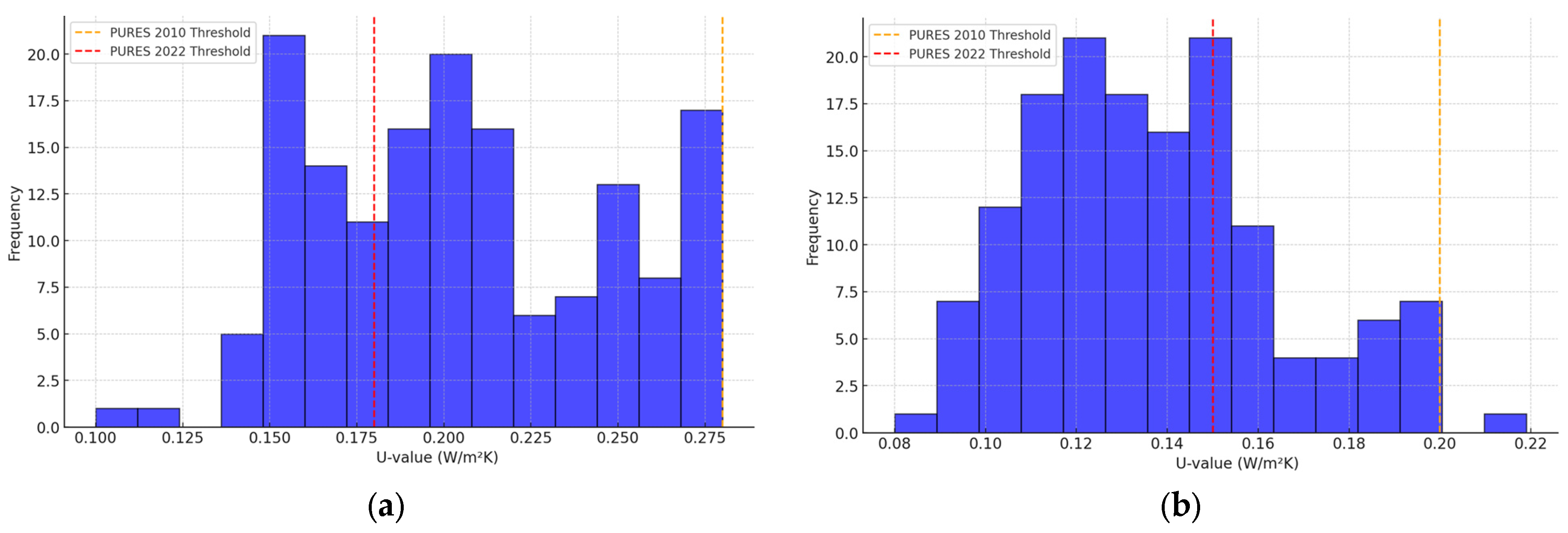
3.1. Findings on U-Value Compliance and Performance
3.2. Comparison of Energy Performance Predictions
3.2.1. Differences in Energy Consumption Estimates Between Static and Dynamic Models
3.2.2. Evaluation of Prediction Errors and Implications on Energy Efficiency Planning
3.3. Impact on CO2 Emission Reductions
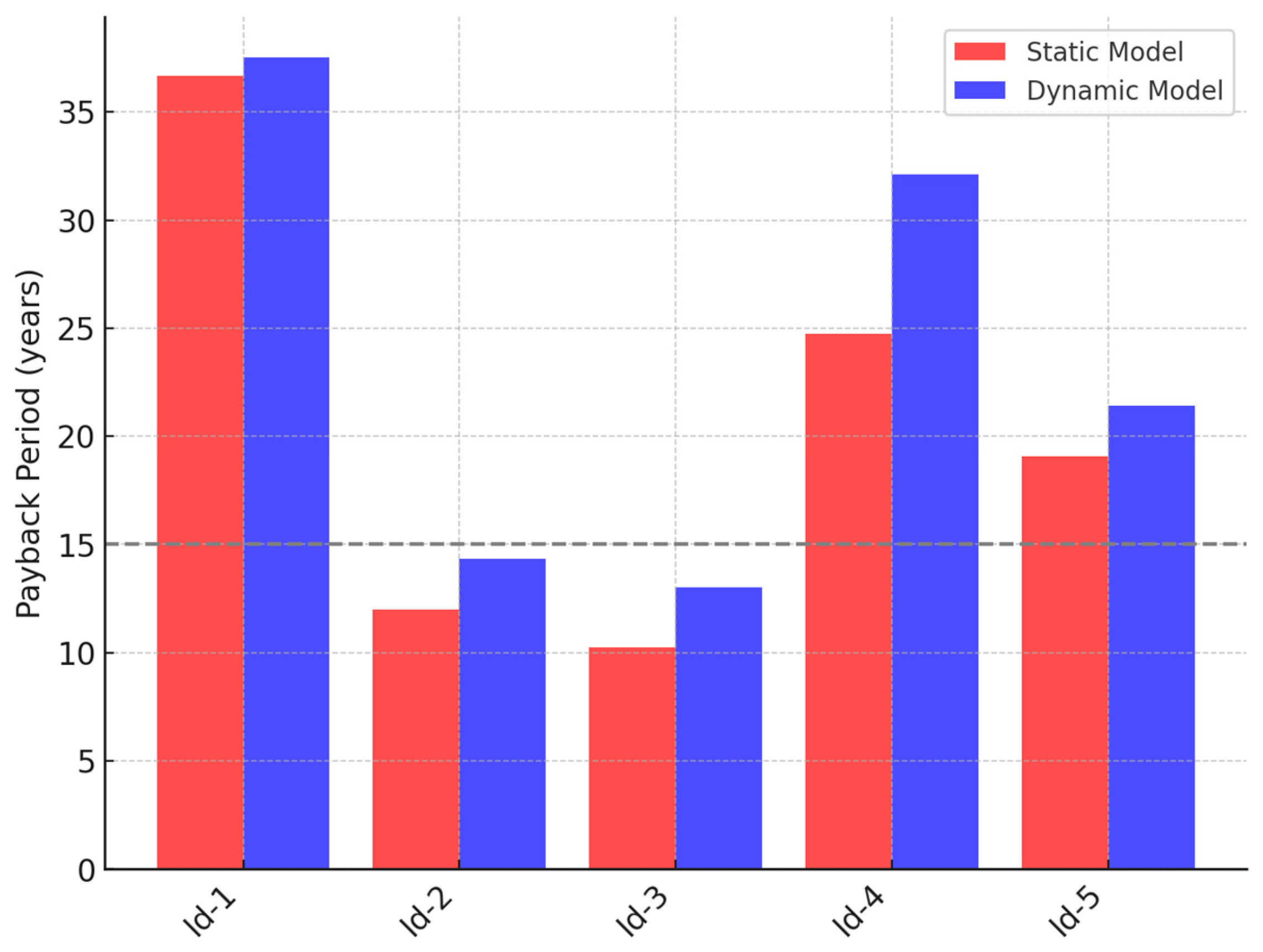
3.4. Financial Implications of Incorrect Simulations
4. Conclusions
Funding
Institutional Review Board Statement
Data Availability Statement
Acknowledgments
Conflicts of Interest
Abbreviations
| BIM | Building Information Modeling |
| BEM | Building Energy Model |
| BPS | Building performance simulation |
| EED | Energy Efficiency Directive |
| EPBD | Energy Performance of Buildings Directive |
| EPC | Energy Performance Certificate |
| ESCO | Energy Services Company |
| GHG | Greenhouse gas |
| HVAC | Heating, ventilation, and air conditioning |
| LED | Light-emitting diode |
| nZEB | Nearly zero-energy buildings |
| PURES | Rules on efficient use of energy in buildings |
| PV | Solar photovoltaic |
| ZEB | Zero-emission buildings |
References
- International Energy Agency (IEA). Buildings—Energy System. Available online: https://www.iea.org/energy-system/buildings (accessed on 5 February 2025).
- European Commission. The European Green Deal. Available online: https://commission.europa.eu/strategy-and-policy/priorities-2019-2024/european-green-deal_en (accessed on 5 February 2025).
- European Commission. 2050 Long-Term Strategy. Available online: https://climate.ec.europa.eu/eu-action/climate-strategies-targets/2050-long-term-strategy_en (accessed on 5 February 2025).
- Bertoldi, P.; Boza-Kiss, B.; Della Valle, N.; Economidou, M. The role of one-stop shops in energy renovation—A comparative analysis of OSSs cases in Europe. Energy Build. 2021, 250, 111273. [Google Scholar] [CrossRef]
- EUR-Lex. Directive—2023/1791—EN. Available online: https://eur-lex.europa.eu/eli/dir/2023/1791/oj/eng (accessed on 5 February 2025).
- Economidou, M.; Todeschi, V.; Bertoldi, P.; D’Agostino, D.; Zangheri, P.; Castellazzi, L. Review of 50 years of EU energy efficiency policies for buildings. Energy Build. 2020, 225, 110322. [Google Scholar] [CrossRef]
- Energy Efficiency Directive. Available online: https://energy.ec.europa.eu/topics/energy-efficiency/energy-efficiency-targets-directive-and-rules/energy-efficiency-directive_en (accessed on 5 February 2025).
- Negendahl, K. Building performance simulation in the early design stage: An introduction to integrated dynamic models. Autom. Constr. 2015, 54, 39–53. [Google Scholar] [CrossRef]
- Harish, V.; Kumar, A. A review on modeling and simulation of building energy systems. Renew. Sustain. Energy Rev. 2016, 56, 1272–1292. [Google Scholar] [CrossRef]
- Arbulu, M.; Oregi, X.; Etxepare, L.; Hernández-Minguillón, R.J. Barriers and challenges of the assessment framework of the Commission Recommendation (EU) 2019/786 on building renovation by European RTD projects. Energy Build. 2022, 269, 112267. [Google Scholar] [CrossRef]
- European Commission. Directive (EU) 2024/1275 of the European Parliament and of the Council of 24 April 2024 on the Energy Performance of Buildings (Recast) (Text with EEA Relevance). 2024. Available online: https://eur-lex.europa.eu/legal-content/EN/TXT/PDF/?uri=OJ:L_202401275 (accessed on 5 February 2025).
- Maduta, C.; D’agostino, D.; Tsemekidi-Tzeiranaki, S.; Castellazzi, L. From Nearly Zero-Energy Buildings (NZEBs) to Zero-Emission Buildings (ZEBs): Current status and future perspectives. Energy Build. 2024, 328, 115133. [Google Scholar] [CrossRef]
- Agliardi, E.; Cattani, E.; Ferrante, A. Deep energy renovation strategies: A real option approach for add-ons in a social housing case study. Energy Build. 2018, 161, 1–9. [Google Scholar] [CrossRef]
- Milić, V.; Ekelöw, K.; Andersson, M.; Moshfegh, B. Evaluation of energy renovation strategies for 12 historic building types using LCC optimization. Energy Build. 2019, 197, 156–170. [Google Scholar] [CrossRef]
- Yin, X.; Muhieldeen, M.W. Evaluation of cooling energy saving and ventilation renovations in office buildings by combining bioclimatic design strategies with CFD-BEM coupled simulation. J. Build. Eng. 2024, 91, 109547. [Google Scholar] [CrossRef]
- Arbulu, M.; Oregi, X.; Etxepare, L.; Fuster, A.; Srinivasan, R.S. Decarbonisation of the Basque Country residential stock by a holistic enviro-economic assessment of renovation strategies under the life cycle thinking for climate risk mitigation. Sustain. Cities Soc. 2024, 117, 105963. [Google Scholar] [CrossRef]
- Seghier, T.E.; Lim, Y.-W.; Harun, M.F.; Ahmad, M.H.; Samah, A.A.; Majid, H.A. BIM-based retrofit method (RBIM) for building envelope thermal performance optimization. Energy Build. 2022, 256, 111693. [Google Scholar] [CrossRef]
- Konstantinou, T.; Knaack, U. An approach to integrate energy efficiency upgrade into refurbishment design process, applied in two case-study buildings in Northern European climate. Energy Build. 2013, 59, 301–309. [Google Scholar] [CrossRef]
- Moran, P.; O’Connell, J.; Goggins, J. Sustainable energy efficiency retrofits as residenial buildings move towards nearly zero energy building (NZEB) standards. Probab. Theory Relat. Fields 2020, 211, 109816. [Google Scholar] [CrossRef]
- Morris, B. The components of the Wired Spanning Forest are recurrent. Probab. Theory Relat. Fields 2003, 125, 259–265. [Google Scholar] [CrossRef]
- Delač, B.; Pavković, B.; Lenić, K.; Mađerić, D. Integrated optimization of the building envelope and the HVAC system in nZEB refurbishment. Appl. Therm. Eng. 2022, 211, 118442. [Google Scholar] [CrossRef]
- Lorenzati, A.; Ballarini, I.; De Luca, G.; Corrado, V. Social Housing in Italy: Energy Audit and Dynamic Simulation Towards a nZEB Policy. In Proceedings of the 16th IBPSA Conference, Rome, Italy, 2–4 September 2019. [Google Scholar]
- Hirvonen, J.; Jokisalo, J.; Heljo, J.; Kosonen, R. Towards the EU emissions targets of 2050: Optimal energy renovation measures of Finnish apartment buildings. Int. J. Sustain. Energy 2018, 38, 649–672. [Google Scholar] [CrossRef]
- Guarino, F.; Tumminia, G.; Longo, S.; Cellura, M.; Cusenza, M.A. An integrated building energy simulation early—Design tool for future heating and cooling demand assessment. Energy Rep. 2022, 8, 10881–10894. [Google Scholar] [CrossRef]
- Wei, C.; Huang, Y.; Löschel, A. Recent advances in energy demand for residential space heating. Energy Build. 2022, 261, 111965. [Google Scholar] [CrossRef]
- Hamid, A.A.; Farsäter, K.; Wahlström, Å.; Wallentén, P. Literature review on renovation of multifamily buildings in temperate climate conditions. Energy Build. 2018, 172, 414–431. [Google Scholar] [CrossRef]
- Beck, H.E.; Zimmermann, N.E.; McVicar, T.R.; Vergopolan, N.; Berg, A.; Wood, E.F. Present and future Köppen-Geiger climate classification maps at 1-km resolution. Sci. Data 2018, 5, 180214. [Google Scholar] [CrossRef]
- Jones, P.D. Instrumental Temperature Change in the Context of the Last 1000 Years. In Detecting and Modelling Regional Climate; Change, M.B., India, D.L., Bonillo, Eds.; Springer: Berlin/Heidelberg, Germany, 2001; pp. 55–68. [Google Scholar] [CrossRef]
- Serra, E.G.; Filho, Z.R.P. Methods for Assessing Energy Efficiency of Buildings. J. Sustain. Dev. Energy Water Environ. Syst. 2019, 7, 432–443. [Google Scholar] [CrossRef]
- Krawczyk, D.A. Theoretical and real effect of the school’s thermal modernization—A case study. Energy Build. 2014, 81, 30–37. [Google Scholar] [CrossRef]
- Calise, F.; Di Vastogirardi, G.N.; D’Accadia, M.D.; Vicidomini, M. Simulation of polygeneration systems. Energy 2018, 163, 290–337. [Google Scholar] [CrossRef]
- Jalalizadeh, M.; Fayaz, R.; Delfani, S.; Mosleh, H.J.; Karami, M. Dynamic simulation of a trigeneration system using an absorption cooling system and building integrated photovoltaic thermal solar collectors. J. Build. Eng. 2021, 43, 102482. [Google Scholar] [CrossRef]
- Calise, F.; Cappiello, F.; Cimmino, L.; Vicidomini, M. Semi-stationary and dynamic simulation models: A critical comparison of the energy and economic savings for the energy refurbishment of buildings. Energy 2024, 300, 131618. [Google Scholar] [CrossRef]
- Kotarela, F.; Kyritsis, A.; Agathokleous, R.; Papanikolaou, N. On the exploitation of dynamic simulations for the design of buildings energy systems. Energy 2023, 271, 127002. [Google Scholar] [CrossRef]
- Li, C.; Prasad, S.; Bai, Y.; Turkeri, C.; Wang, J. A quasi-dynamic model and comprehensive simulation study of district heating networks considering temperature delay. Energy 2025, 318, 134855. [Google Scholar] [CrossRef]
- Mora, T.D.; Peron, F.; Romagnoni, P.; Almeida, M.; Ferreira, M. Tools and procedures to support decision making for cost-effective energy and carbon emissions optimization in building renovation. Energy Build. 2018, 167, 200–215. [Google Scholar] [CrossRef]
- EN ISO DIS 13790; Energy Performance of Buildings–Calculation of Energy Use for Space Heating and Cooling. ISO: Geneva, Switzerland, 2007.
- Stegnar, G.; Staničić, D.; Česen, M.; Čižman, J.; Pestotnik, S.; Prestor, J.; Urbančič, A.; Merše, S. A framework for assessing the technical and economic potential of shallow geothermal energy in individual and district heating systems: A case study of Slovenia. Energy 2019, 180, 405–420. [Google Scholar] [CrossRef]
- Zavrl, M.Š.; Stegnar, G.; Rakušček, A.; Gjerkeš, H. A Bottom-Up Building Stock Model for Tracking Regional Energy Targets—A Case Study of Kočevje. Sustainability 2016, 8, 1063. [Google Scholar] [CrossRef]
- Portal Energetika—Projektna Pisarna za Energetsko Prenovo Stavb (PP—EPS). Available online: https://www.energetika-portal.si/podrocja/energetika/energetska-prenova-javnih-stavb/projektna-pisarna/ (accessed on 18 February 2025).


| Building Component | PURES 2010 Limit [W/m2K] | PURES 2022 Limit [W/m2K] |
|---|---|---|
| Façade | 0.28 | 0.18 |
| Windows | 1.30 | 1.00 |
| Roof | 0.20 | 0.15 |
| Floors | 0.30 | 0.35 |
| Building Id | Photo | Model |
|---|---|---|
| Id-1 | 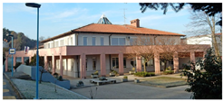 | 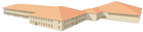 |
| Id-2 | 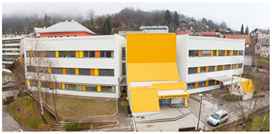 |  |
| Id-3 | 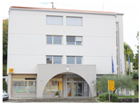 | 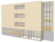 |
| Id-4 | 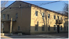 | 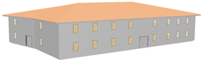 |
| Id-5 | 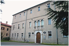 |  |
| Building Id | Type | Year Built | Conditioned Area [m2] | Renovation Measures (Actual or Proposed) | Energy Data Used |
|---|---|---|---|---|---|
| Id-1 | Elementary School | 1976 (partly renovated 1994) | 3174 | Insulation, window replacement, LED lighting, heat pump | EPC, BIM, Energy Audit, Consumption Data |
| Id-2 | Health Center | 1980 (renovated 2019) | 3630 | Heating system upgrade, district heating, energy management system | EPC, BIM, Energy Audit, Consumption Data |
| Id-3 | Office Building | 1956 (renovated 2013) | 605 | ESCO model, energy monitoring, lighting retrofit | EPC, BIM, Energy Audit, Consumption Data |
| Id-4 | School | 1675 (façade renovated 1970, roof 1994) | 2527 | Cultural heritage constraints, energy-inefficient systems | EPC, BIM, Energy Audit, Consumption Data |
| Id-5 | Elementary School | 1960 (renovated 2022) | 3977 | Insulation, LED lighting, district heating, PV system | EPC, BIM, Energy Audit, Consumption Data |
| Building Component | Average U-Value [W/m2K] | PURES 2010 Limit [W/m2K] | PURES 2022 Limit [W/m2K] | Compliance Observation |
|---|---|---|---|---|
| Façade | 0.205 | 0.28 | 0.18 | Partial compliance, requires additional retrofits |
| Windows | 1.087 | 1.30 | 1.00 | High variability, inconsistent compliance with PURES 2022 |
| Roof | 0.136 | 0.20 | 0.15 | Strong compliance across most projects |
| Floors | 0.259 | 0.30 | 0.35 | Generally compliant, though some projects exceed thresholds |
| Building Code | Static Model [kWh/m2a] | Dynamic Model [kWh/m2a] | Absolute Error [kWh/m2a] | Relative Error [%] |
|---|---|---|---|---|
| Id-1 | 75.0 | 63.3 | 11.7 | 15.6 |
| Id-2 | 95.6 | 80.0 | 15.6 | 16.3 |
| Id-3 | 32.3 | 23.8 | 8.5 | 26.3 |
| Id-4 | 102.2 | 64.6 | 37.6 | 36.8 |
| Id-5 | 115.2 | 86.1 | 29.1 | 25.3 |
Disclaimer/Publisher’s Note: The statements, opinions and data contained in all publications are solely those of the individual author(s) and contributor(s) and not of MDPI and/or the editor(s). MDPI and/or the editor(s) disclaim responsibility for any injury to people or property resulting from any ideas, methods, instructions or products referred to in the content. |
© 2025 by the author. Licensee MDPI, Basel, Switzerland. This article is an open access article distributed under the terms and conditions of the Creative Commons Attribution (CC BY) license (https://creativecommons.org/licenses/by/4.0/).
Share and Cite
Stegnar, G. Bridging the Gap to Decarbonization: Evaluating Energy Renovation Performance and Compliance. Energies 2025, 18, 1146. https://doi.org/10.3390/en18051146
Stegnar G. Bridging the Gap to Decarbonization: Evaluating Energy Renovation Performance and Compliance. Energies. 2025; 18(5):1146. https://doi.org/10.3390/en18051146
Chicago/Turabian StyleStegnar, Gašper. 2025. "Bridging the Gap to Decarbonization: Evaluating Energy Renovation Performance and Compliance" Energies 18, no. 5: 1146. https://doi.org/10.3390/en18051146
APA StyleStegnar, G. (2025). Bridging the Gap to Decarbonization: Evaluating Energy Renovation Performance and Compliance. Energies, 18(5), 1146. https://doi.org/10.3390/en18051146