Optimized Strategy for Energy Management in an EV Fast Charging Microgrid Considering Storage Degradation

Abstract

Current environmental challenges demand immediate action, especially in the transport sector, which is one of the largest CO₂ emitters. Vehicle electrification is considered an essential strategy for emission mitigation and combating global warming. This study presents methodologies for the modeling and energy management of microgrids (MGs) designed as charging stations for electric vehicles (EVs). Algorithms were developed to estimate daily energy generation and charging events in the MG. These data feed an energy management algorithm aimed at minimizing the costs associated with energy trading operations, as well as the charging and discharging cycles of the battery energy storage system (BESS). The problem constraints ensure the safe operation of the system, availability of backup energy for off-grid conditions, preference for reduced tariffs, and optimized management of the BESS charge and discharge rates, considering battery wear. The grid-connected MG used in our case study consists of a wind turbine (WT), photovoltaic system (PVS), BESS, and an electric vehicle fast charging station (EVFCS). Located on a highway, the MG was designed to provide fast charging, extending the range of EVs and reducing drivers’ range anxiety. The results of this study demonstrated the effectiveness of the proposed energy management approach, with the optimization algorithm efficiently managing energy flows within the MG while prioritizing lower operational costs. The inclusion of the battery wear model makes the optimizer more selective in terms of battery usage, operating it in cycles that minimize BESS wear and effectively prolong its lifespan.

1. Introduction

The global imperative to mitigate greenhouse gas emissions has intensified the efforts being made toward sustainable energy transitions, with the transportation sector playing a key role. According to the International Energy Agency (IEA), energy-related CO₂ emissions reached a record high of 37.4 billion tonnes in 2023, underscoring the urgent need for decarbonization strategies [1]. The transportation sector consumes over 30% of the world’s energy and contributes significantly to CO₂ emissions, accounting for nearly 20% of the total. Among the various modes of transport used, road transport remains the predominant source of greenhouse gas emissions within this sector [2].

Electric vehicles (EVs) have emerged as a cornerstone of this transition, with accelerating worldwide adoption. In Brazil, the EV market, though currently representing a modest share of all automobile sales, has exhibited significant growth. Projections indicate that the Brazilian electric vehicle market is expected to grow by 17.1% on an annual basis, reaching USD 1.2 billion by the end of 2024 [3]. The IEA projects that by 2035 the number of EVs in the world will reach 525 million, and one in four vehicles will be electric [4].

The expansion of the EV fleet necessitates a corresponding development in charging infrastructure, particularly along highways, to support long-distance travel. The integration of distributed energy resources (DERs) into these charging stations presents us with an opportunity to enhance sustainability but also introduces challenges such as managing intermittent generation and preventing reverse power flows during peak production periods [5].

Effective energy management systems (EMS) are essential to address these challenges, as they can optimize the interaction between distributed generation (DG), battery energy storage systems (BESS), and the grid. A critical aspect of EMS optimization involves accounting for storage degradation, which impacts both the economic and operational efficiency of EV fast charging stations (EVFCSs).

This study proposes an optimized EMS strategy for fast charging microgrids for EVs that incorporates storage degradation considerations. By leveraging predictive algorithms and real-time data, the proposed system aims to enhance energy efficiency, reduce operational costs, and extend the lifespan of its storage components, thereby contributing to the sustainable expansion of EV infrastructure in Brazil and beyond.

1.1. Highlights of This Paper

Some of the contributions of this paper are as follows:

• The integration of load, generation, and storage elements, including an EVFCS, BESS, PV, and WT, in the proposed microgrid (MG) framework.
• The utilization of Time-of-Use (ToU) tariffs allows the exploration of additional pricing mechanisms, such as Day-Ahead Market tariffs, for cost optimization.
• An objective function focused on minimizing MG operational costs by prioritizing BESS usage and the consumption of locally generated energy.
• The inclusion of BESS degradation in the optimization problem to ensure realistic and sustainable storage management.
• A flexible and modular design, which allows scalability to larger problems and the incorporation of additional components within the MG.
• The modeling approach is based on Python, leveraging free algorithms, packages, and solvers to promote its accessibility and replicability.
• Renewable generation estimation based on meteorological forecasts combined with physical models, improving prediction accuracy.
• Load consumption estimation leveraging historical data from EVFCS operations, enabling more accurate forecasts as usage patterns evolve.
• Modular models for the generation, charging, and EMS algorithms used, allowing seamless updates and their replacement with improved versions.

1.2. Limitations of This Paper

Although this paper proposes highly flexible methodologies that can be adapted to other scenarios and studies, it is important to highlight some limitations:

• Our model is developed for highway scenarios, where the dynamics of FCSs focus on avoiding queue formation, prioritizing quick charging sessions without considering extended parking times or energy exchanges via vehicle-to-grid (V2G) modes.
• Future applications may partially leverage the methodologies developed here for urban parking or rural contexts, adjusting them to meet the specific needs of these scenarios.
• The primary focus of this paper is the EMS, with other topics related to MG operation falling outside the scope of this study.

2. Analysis and Contextualization of the Literature

The incorporation of renewable energy resources has led to a significant rise in the deployment of DERs within energy systems. These DERs, when combined with associated loads, constitute an MG [6]. As defined by the National Renewable Energy Laboratory (NREL), an MG is a system comprising interconnected loads and DERs that function as a unified controllable entity relative to the main power grid. This system can operate in two distinct modes: grid-connected, where it interfaces with the main grid, or islanded, where it functions independently [7].

Considering the increasing adoption of MGs, the development of usage and management strategies for these systems has become a critical requirement. In the literature, optimization problems are commonly addressed, with objectives such as minimizing costs, energy losses, or recharge times, as well as maximizing profits, energy sales, efficiency, renewable energy utilization, and other performance metrics [6].

Reference [8] proposes a method of MG management that maximizes discharge/charge rates based on tariff preferences. The generation of DERs is based on typical profiles. In [9], a new battery wear model is based on a V2G application model, which was adapted for use in MGs. It calculates wear costs based on changes in the state of charge (SoC) during discharge/charge events. A WT is not incorporated in the work.

The authors of [10] present a new scheduling methodology that considers the depth of discharge (DoD) and SoC levels to minimize battery degradation, achieving a reduction in the capacity loss of more than 30% in simulations. The applications of this study involve V2G transactions, which do not apply to road contexts.

One study [11] developed a planning strategy for EV charging stations to maximize operator profits, considering investment costs, revenue, and variable costs, using an algorithm that iteratively adds stations to meet charging needs while optimizing facility utilization. The system proposed by [12] is designed for MGs operating in isolated areas and utilizes a Renewable-Based Energy Management System (RBEMS) that analyzes historical data and short-term forecasts to determine set points for renewable generation and programmable loads in a cost-effective, reliable, and sustainable manner.

On the other hand, some studies are focused on the residential context, such as study [13], which explores energy management options for EV charging stations in buildings, with a focus on increasing their power grid capacity without increasing peak demand. It emphasizes adaptable solutions to seasonal and daily demand variations, promoting sustainable transport ecosystems in urban areas.

Some research works on energy management, considering the charging stations in cities. Paper [14] features a cost-effective energy management system for fast charging stations that integrates solar PV and energy storage systems. It focuses on optimizing the charging of electric vehicles in urban environments, increasing sustainability and reducing reliance on fossil fuels. In addition to not considering WTs, the implementation of the EMS is achieved via commercial software, which can result in additional costs for the operator. Many studies do not consider the allocation of a BESS, while others only look at the integration of fast-charging EVs with PVS plants [15].

Classical programming methods are quite common in the literature for the modeling and operation of EMSs, as is the case in [16], which discusses the optimal planning and dispatch of BESSs in MGs, with a focus on improving their cycle life through a mathematical model formulated as a Mixed Integer Linear Programming (MILP) problem and solved using GUROBI. The study was validated in a test MG. Like the other papers presented, its dependence on commercial solvers can lead to unforeseen expenses.

EMSs for EVFCSs along highways are essential to optimizing the operational efficiency, reliability, and sustainability of charging infrastructure. These systems leverage advanced control strategies to address critical challenges such as peak demand mitigation, cost minimization, and grid stability enhancement. Their core functionalities include real-time load balancing to prevent grid overloading, the integration of DERs to reduce emissions, and the utilization of an energy storage system (ESS) to buffer demand fluctuations. Predictive algorithms and demand forecasting are employed to optimize energy allocation, minimizing charging times and enhancing user satisfaction. Through these integrated strategies, an EMS for EVFCSs facilitates the scalable and sustainable expansion of electrified highway systems [17,18].

Other approaches consider the energy management of an island group energy system, as in [19]. The article introduces a Hybrid Policy-based Reinforcement Learning (HPRL) approach for adaptive energy management in energy transmission-constrained island groups. It proposes an Insular Energy Hub (IEH) model that enables cascading energy utilization, addressing the specific energy demands of islands while ensuring supply reliability. Furthermore, the Energy Management Model for Island Groups (EMIG) is formulated to account for the inverse distribution of demand and energy resources, transforming the challenge into a model-free reinforcement learning task. The effectiveness of the approach was demonstrated through numerical simulations. For now, the focus of the optimization in this paper is on grid-connected operation within a single MG. Future research may address energy management while considering more MGs and their cooperation to meet the goals at reduced costs.

Taking into account these findings and the possible deficiencies found in the literature, this study proposes the programmed management of an MG. Here, DER generation models are updated daily, based on predicted weather data, and obtained via reliable Application Programming Interfaces (APIs) [20]. This provides better assertiveness, since the generation of these plants is correlated with meteorological data [21]. Weather models have evolved significantly and are now widely used for accurate weather and weather-related forecasts. In addition, the integration of a BESS contributes to increasing the reliability of the MG and ensuring that it is able to operate even when off-grid. The consideration and implementation of a BESS wear model contribute to a more balanced use of the system, avoiding overuse and premature end-of-life.

The inclusion of hourly tariffs enables the EMS to make informed decisions aimed at reducing energy costs by purchasing electricity during lower-cost periods. The modularity of the EMS algorithm’s input data facilitates the continuous calibration and improvement of each submodel within the overall model. The proposed EMS also accommodates updates to capture metering value discounts for sold energy. Furthermore, two options are presented to estimate charging demand in the EVFCS. The first option provides estimations for initial operations, where the station’s usage patterns are yet unknown. The second option allows for updates based on an established database, enabling the estimation of the EVFCS load curve by analyzing the trends observed in historical data.

3. Proposed Methodology

Our proposed methodology for MG management integrates meteorological data and mathematical models to predict the energy generated from renewable sources throughout the day. In addition, the values of the electricity tariff and the EV recharging events estimated for the day of operation are considered. Based on this estimated information, the dispatch of the BESS is programmed using the energy management algorithm. The dispatch profile resulting from this optimization is sent, via the internet, to the MG’s central industrial computer, which passes the defined set points to the Programmable Logic Controller (PLC), which controls BESS dispatches throughout the day. Figure 1 presents a schematic summary of this entire methodology.

The following subsections show the modeling carried out to estimate the recharges in the MG and the generations coming from WTs and PVSs, the BESS wear model is detailed, and later the algorithm developed to optimize energy management in the MG is presented.

3.1. EVFCS Usage Modeling

Forecasting and analyzing the demand for EV charging on highways faces significant challenges, as it relies on several external and unpredictable factors, such as mobility patterns, seasonality, weather, and human behavior. To address these uncertainties, several models have been developed, including approaches based on statistical data, which learn from historical usage patterns, traffic surveys, and vehicle flow counts, among other data.

In [22], a methodology is presented that models typical vehicle usage profiles in Brazil, categorized according to the types of trips undertaken, enabling the estimation of charging demand. In turn, study [23] builds upon these typical usage profiles for regular users and complements the analysis by including occasional users, modeled through simulations based on the Monte Carlo method. However, both approaches are focused on charging in residential contexts and parking lots, and do not consider the specificities of charging behavior on highways, which requires a different analysis due to its unique characteristics and greater variability.

In the context of highways, two possible alternatives can be highlighted. The first is intended for initial EVFCS operations, for which a consolidated history of recharging data is not yet available. The second leverages observed patterns in recharging behavior, such as energy consumption, recharge duration, and connection time. Therefore, at first, the methodology developed in [24] should be used, since there is no history of recharges. The daily capacity behavior of the establishment, the typical variations in flow on the highway, the market share of EVs, and the distribution of the battery capacities of the EVs sold serve as a basis for estimating recharging events and then the EVFCS usage pattern [24].

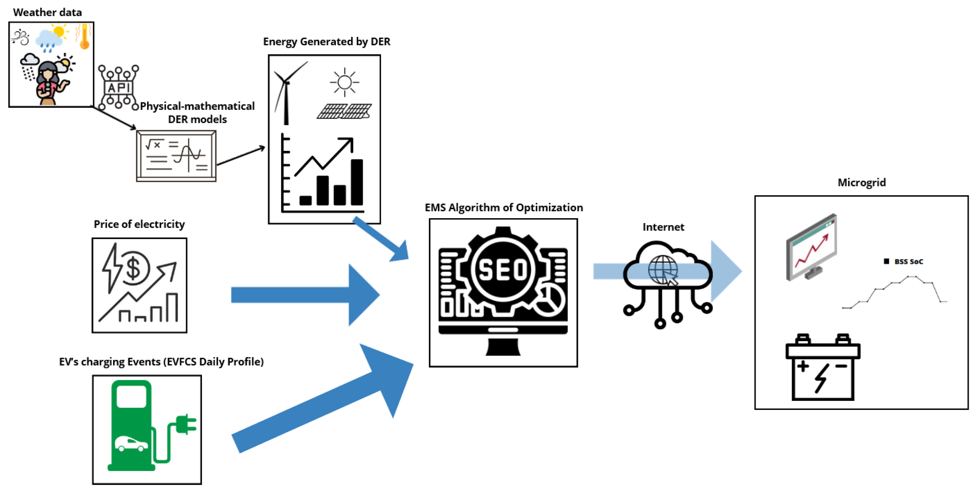
As a second option, when the user’s behavior is already known, the EVFCS demand curve can be obtained from the statistics of their recharge history. This is a more attractive option and it will be used in this work. The algorithm developed follows the following step-by-step list, which is also illustrated in Figure 2:

• Load and Clear Data: Organize historical data.
• Filter Relevant Data: Eliminate database errors, erroneous data, and outliers.
• Analyze Trends: Identify historical patterns.
• Generate Usage Profile: Create probabilistic models.
• Simulate Scenarios: Generate daily recharge distributions based on historical patterns.
• Preview Results: Show the simulated and average curves.
• Export Data: Save results for integration with other systems.

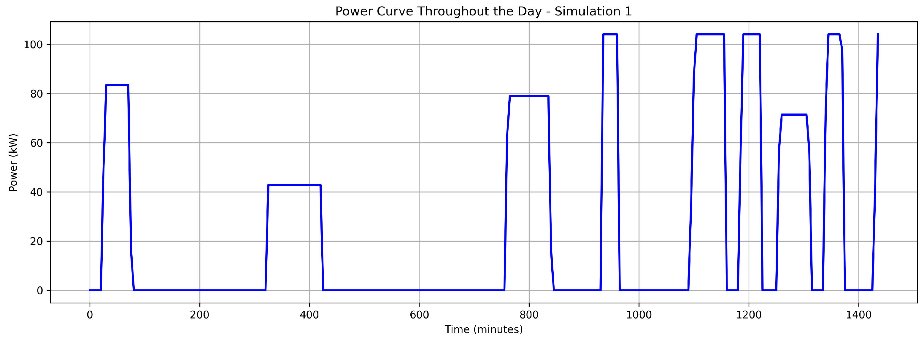
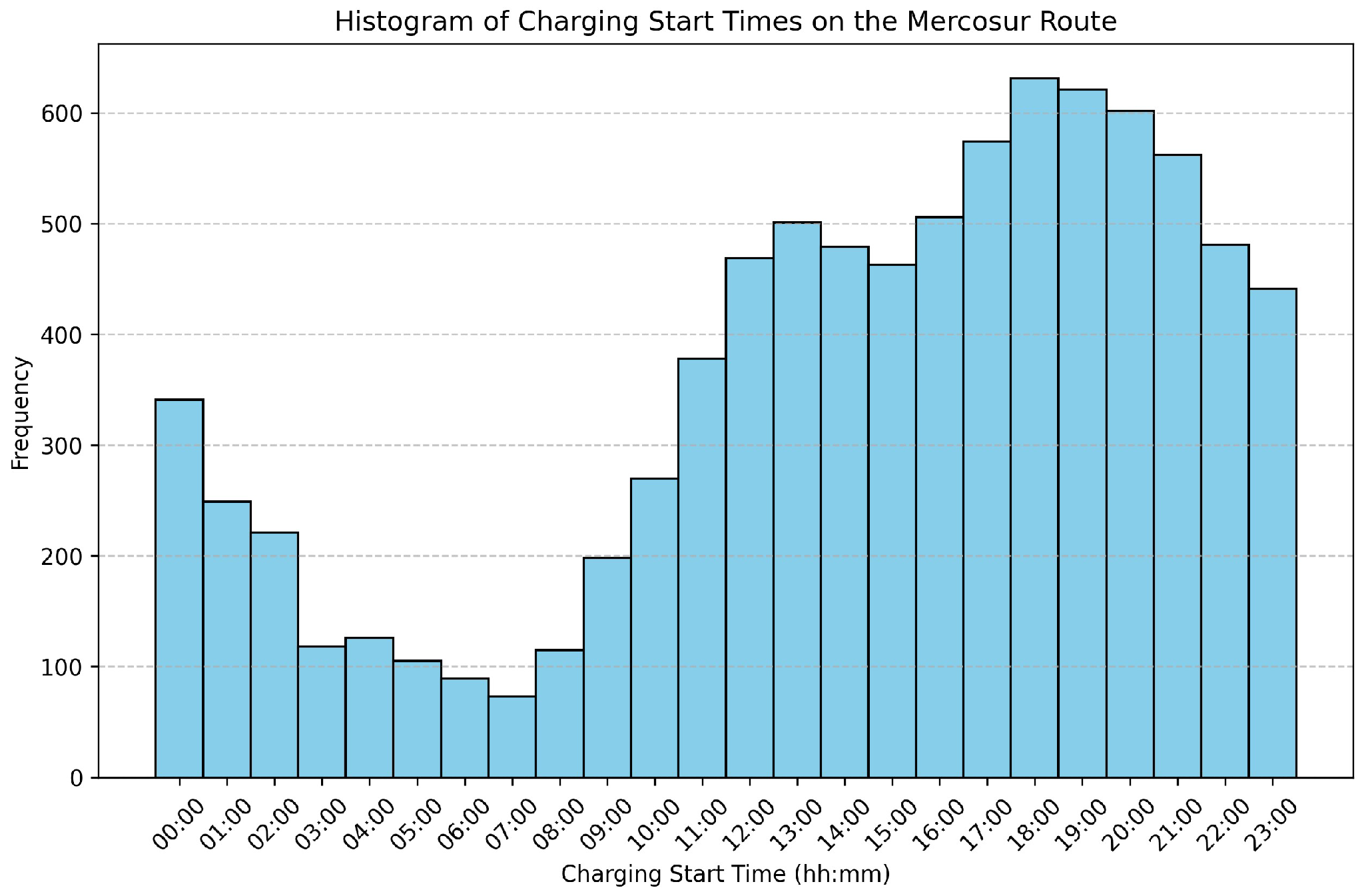
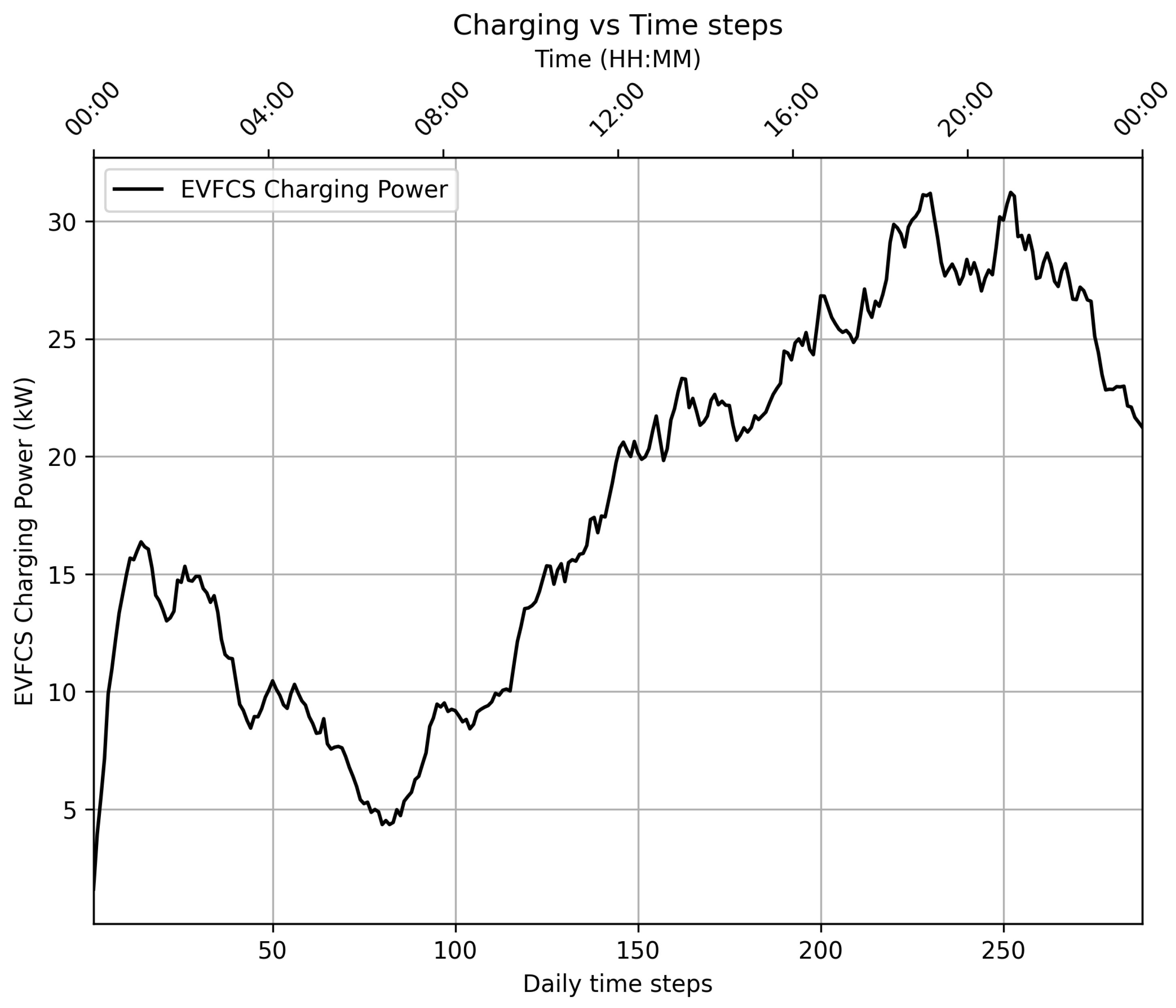
Figure 3 shows a daily recharge profile obtained by following the process described above. This profile was generated from historical recharge data, which were organized, filtered, and analyzed to identify patterns of behavior. Subsequently, probabilistic modeling was used to create representative distributions of the characteristics of the recharges, such as their duration, energy consumed, and start times. Based on these distributions, daily scenarios were simulated that reflect the typical use of an EVFCS. Finally, the results were viewed and exported for integration into the EMS algorithm.

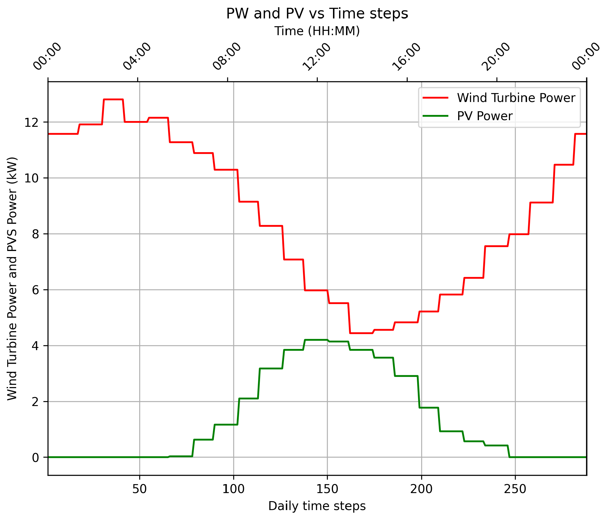
3.2. Wind Generation Modeling

The use of wind kinetics for the generation of electricity depends on factors such as the wind speed; turbine sweep area; characteristics of the installation site, such as soil roughness and altitude; and the construction characteristics of the WT [25,26,27].

There are different types of models used for wind generation forecasting. The main ones used include physical, statistical, and hybrid models. Physical models are based on the principles of fluid mechanics and the technical characteristics of the turbines, such as the power curve and the geometry of the blades, and are fed meteorological data, such as wind speed and direction, obtained from numerical forecasts or local measurements [28,29].

Statistical models, on the other hand, use methods such as linear regression and time series to identify historical patterns, offering quick solutions but with limitations in scenarios of high variability. Hybrid models combine physical and statistical approaches, using machine learning techniques to capture the complex relationships between the variables involved [28,29]. The choice of model depends on accuracy requirements, time horizon, and data availability, with physical models standing out for their robustness when fed with detailed weather forecasts.

Deterministically, it is possible to calculate the mechanical power available in a wind turbine using Equation (1):

$$P_{\mathrm{turb}}={\displaystyle \frac{1}{2}}·\rho ·C_p·A·v_1^3$$

(1)

where $P_{\mathrm{turb}}$ is the mechanical power of the turbine (W, kW, or MW), $\rho$ is the air density (kg/m³), $C_p$ is the power coefficient of the turbine or Betz limit, A is the rotor area (m²), and $v_1$ is the velocity of the wind approaching the turbine (m/s). The air density is approximately 1.225 kg/m³ under standard temperature and pressure conditions (1 atm, 15.56 °C, at sea level). References [25,30] highlight that it is possible to estimate the air density based on the altitude of a location, when necessary. The higher the altitude, the more rarefied the air becomes, leading to a lower density [25,30].

Consequently, the electrical power generated by a WT is given by Equation (2):

$$P_{\mathrm{elet}}=P_{\mathrm{turb}}·{\eta }_t$$

(2)

where $P_{\mathrm{elet}}$ is the electrical power delivered (W, kW, or MW) and ${\eta }_t$ is the total efficiency of the wind turbine system, including components such as the generator, gearbox, mechanical losses, and electrical losses [25].

It is also possible to calculate the power generated by the wind turbine through the turbine power curve provided by the manufacturer from tests. This curve relates the output power generated to the wind speed incident on the turbine blades. Figure 4 shows a power curve that is a function of wind speed for a 30 kVA WT.

Wind power generation is only possible above a minimum wind speed (cut-in speed) and varies with the wind speed and turbine characteristics until reaching the cut-out speed, at which point the turbine must be shut down. The wind speed at the turbine blades must be adjusted, as API data typically provide wind speeds measured at 10 m above the ground. The Hellman Law is widely used in engineering and meteorology to extrapolate wind speeds from a reference height $z_0$ to a height z, considering the properties of the terrain and the logarithmic wind profile. This law provides a practical way of estimating wind speeds at different heights based on terrain roughness [27,31]. The basic formula of the Hellman Law is expressed in Equation (3).

$$v\left(z\right)=v\left(z_0\right)·{\left({\displaystyle \frac{z}{z_0}}\right)}^{{\alpha }_h}$$

(3)

In Equation (3), $v\left(z\right)$ represents the wind speed at height z (in m/s), while $v\left(z_0\right)$ is the wind speed at the reference height $z_0$ (in m/s). The variable z denotes the height at which the wind speed is to be extrapolated (in meters), and $z_0$ is the reference height, where the wind speed is already known (in meters). The exponent ${\alpha }_h$ depends on the roughness of the terrain and is an empirical parameter that varies with the type of terrain and atmospheric conditions.

The value of ${\alpha }_h$ typically varies depending on the roughness of the terrain. For example, for water surfaces or very flat terrains, ${\alpha }_h\approx 0.10$. In rural areas or regions with low vegetation, ${\alpha }_h\approx 0.15$. In suburban areas or regions with medium-sized constructions, ${\alpha }_h\approx 0.25$. Finally, for urban areas or regions with tall buildings, ${\alpha }_h\approx 0.30$. The Hellman Law is a practical tool for estimating wind speeds at various heights. However, its accuracy depends on the assumption of a constant wind profile and the consistency of terrain roughness. Abrupt changes in terrain or atmospheric instability can reduce the precision of this method.

Via a weather API, wind speed forecasts are obtained for the next day. Data interpolation manipulations are performed every 5 min, and the wind speed is corrected, via Hellman’s Law, to the height of the wind turbine. Thus, it is possible to calculate the generation of power, as shown in the diagram in Figure 5.

3.3. PV Generation Modeling

Photovoltaic generation forecasting methods are widely used to optimize the use of solar energy and are divided into three main approaches: those based on physical models, statistical methods, and artificial intelligence techniques. Physical models use meteorological information, such as solar radiation and ambient temperature, and the characteristics of photovoltaic systems to estimate energy generation based on physical principles. Statistical methods, on the other hand, apply time series and mathematical models, such as linear regression and ARIMA, to identify historical patterns and make short-term predictions [32,33,34].

On the other hand, artificial intelligence techniques such as Artificial Neural Networks (ANNs), machine learning, and hybrid algorithms offer more accurate forecasts by learning from large volumes of historical and weather data. The combination of physical models of the panels with weather forecast data has significant advantages, such as greater accuracy when incorporating real-time weather conditions or day-ahead forecasts and adaptability to local variations, allowing you to optimize energy generation and plan more efficiently and reliably [32,33,34].

The calculation of photovoltaic generation is based on the nominal power of the module, the rate of the reduction in the efficiency of the photovoltaic module due to degradation, solar irradiation at the installation site, and the temperature of the module, as shown in Equation (4) [33,35].

$$P_{\mathrm{PV},\mathrm{un}}\left(h\right)=Y_{\mathrm{PV}}·f_{\mathrm{PV}}·{\displaystyle \frac{G_T\left(h\right)}{G_{T,\mathrm{STC}}}}·\left[1+{\alpha }_p·\left(T_C\left(h\right)-T_{C,\mathrm{STC}}\right)\right]$$

(4)

where $P_{\mathrm{PV},\mathrm{un}}\left(h\right)$ is the output power of the photovoltaic module (kW) at hour h, $Y_{\mathrm{PV}}$ is the nominal power of the photovoltaic module under standard test conditions (kW); $f_{\mathrm{PV}}$ is the efficiency reduction factor of the photovoltaic module due to degradation (%); $G_T\left(h\right)$ is the total irradiance on the surface of the Earth (W/m²) at hour h; $G_{T,\mathrm{STC}}$ is the irradiance under standard test conditions, assumed to be 1000 W/m²; ${\alpha }_p$ is the power temperature coefficient (%/°C); $T_C\left(h\right)$ is the photovoltaic panel temperature (°C) at hour h; and $T_{C,\mathrm{STC}}$ is the photovoltaic panel’s temperature under standard test conditions, assumed to be 25 °C [33]. All parameters under standard test conditions (STCs) correspond to those tested by manufacturers in laboratory conditions.

The modeling of the cell temperature in the photovoltaic panel is directly related to the ambient temperature and solar irradiance. Equation (5) presents this approach, where $T_{\mathrm{amb}}\left(h\right)$ is the ambient temperature measured at hour h, $G_T\left(h\right)$ is the hourly irradiance, and NOCT is the nominal operating cell temperature of the photovoltaic panel [36,37].

$$T_C\left(h\right)=T_{\mathrm{amb}}\left(h\right)+{\displaystyle \frac{G_T\left(h\right)}{800}}·(\mathrm{NOCT}-20)$$

(5)

Finally, the output power per photovoltaic panel was estimated using Equation (4); the total power generated is proportional to the power of each panel and the number of panels installed, $N_{\mathrm{PV}}$, as shown in Equation (6). It is worth mentioning that the photovoltaic generation model considers panels with the same generation capacity, positioned similarly, and under similar conditions, accounting for shading and surface states.

$$P_{\mathrm{PV}}\left(h\right)=P_{\mathrm{PV},\mathrm{un}}\left(h\right)·N_{\mathrm{PV}}$$

(6)

This mathematical approach aligns with the methodology employed by Homer software, version 3.14.2, to calculate a plant’s photovoltaic generation. $G_T$ can be inserted into the software as a text file with hourly data, generated from Typical Meteorological Year (TMY) data for the location. In the absence of such data, Homer uses the Graham algorithm to generate synthetic irradiance series [38]. This algorithm produces hourly irradiance values based on the latitude and monthly average irradiance values. Therefore, it allows for energy estimates over long periods.

However, in the short term, the data obtained via a weather API for the next day ensures better accuracy and precision in estimating the photovoltaic generation profile. The sequence of steps followed is shown in Figure 6. Since the data come in every hour, some manipulations and interpolations are required to obtain a daily profile with 5 min discretization, which will be the resolution used in the optimization algorithm.

3.4. BESS Degradation Cost Model

A BESS is costly, especially considering their limited lifespan, as batteries can only endure a finite number of charge–discharge cycles before reaching their End-of-Life (EoL), typically defined as a 20–30% reduction in their State of Health (SoH) [39]. The degradation of Li-ion batteries occurs as a function of variables such as temperature, the calendar effect, the intensity of discharges, and applied currents, among other factors, according to [40,41,42,43]. Among the available technologies, lithium-ion batteries (LIBs) and lead-acid batteries are predominant in modern BESS applications.

Various models are used in the literature to predict and mitigate battery degradation. Empirical and semi-empirical models are widely used due to their simplicity and ability to provide quick estimates based on experimental data. These models correlate the number of charge–discharge cycles with the depth of the discharge and temperature. This work uses the modeling presented by [9], which updates the empirical battery wear model proposed by [44] by considering the battery’s wear as a function of the intensity of the discharge. So, the total cycles of a battery are reduced when it is subjected to a high DoD.

In the literature, some functions have been proposed that relate the Achievable Cycle Count (ACC) to the DoD. Since life cycle data are often presented at discrete DoD levels, interpolation is useful. To achieve this, a generic function $ACC\left(DoD\right)$ can be defined in various formats to fit different wear curves. In [44], the reciprocal function $ACC\left(DoD\right)=a_0·Do{D}^{-a_1}$ is proposed, where $a_0$ and $a_1$ are curve-fitting coefficients, but it has limitations in its universality. Alternative formats, such as the exponential $ACC\left(DoD\right)=a_0·e^{-a_1·DoD}$ and logarithmic $ACC\left(DoD\right)=a_0-a_1·ln\left(DoD\right)$, also fit specific cases well but fail to generalize. To address this, a combined reciprocal and exponential model was proposed by [9] for broader applicability, as shown in Equation (7).

$$ACC\left(DoD\right)=a_0·d^{-a_1}·e^{-a_2·d}$$

(7)

where $a_0$, $a_1$, and $a_2$ are coefficients that can be obtained by methods such as least squares fitting and d is the DoD of the BESS. Considering the cost, capacity, and ACC vs. DoD curve of the BESS, and performing the necessary mathematical manipulations, ref. [9] derived a Normalized Wear Density Function, $w_n\left(s\right)$, expressed in terms of the monetary cost per unit of energy transferred (typically BRL/kWh), as shown in Equation (8). This formula allows you to calculate the density of wear as the DoD varies.

$$w_n\left(s\right)={\displaystyle \frac{\alpha ·B_p}{2·M}}·{\displaystyle \frac{a_1·{(1-s)}^{a_1-1}+a_2·{(1-s)}^{a_1}}{a_0}}·e^{a_2(1-s)}$$

(8)

where $\alpha$ is a modulating factor to account for temperature fluctuation, calculated as $\alpha =e^{0.0035·|T_B-25|}$, where $T_B$ is the temperature of the battery in Celsius. The $B_p$ is the BESS price (BRL), M represents the BESS capacity (kWh), and $(1-s)$ is the current DoD of the BESS.

The average value of the wear density function is useful for assessing the cost–benefit of different battery models, as it considers not only price and capacity but also durability. The average value of Equation (8) is calculated using Equation (9):

$${\overline{w}}_n={\displaystyle \frac{\alpha ·B_p}{2·M}}·{\displaystyle \frac{e^{a_2}}{a_0}}$$

(9)

Since $w_n\left(s\right)$ has nonlinear variation behavior as a function of the SoC, it is necessary to use a piecewise linearization algorithm to insert this variable into linear optimization problems [45].

3.5. Proposed Optimization Algorithm

Our main objectives are an optimized power distribution between the grid and BESS, taking into account the utilization of locally produced renewable energy, and the reduction of operating costs. Therefore, the controllable power rate defines when the BESS charges or discharges energy. These are the decision variables for the optimization problem. This formulation was chosen for its maturity, the availability of such tools, and its fast and robust convergence to the global optimum.

A formal description of this optimization requires the definition of the following parameters and variables, as summarized in

Table 1. Notation for the optimization problem.

Type	Name	Description
Set	T	Time (discretization: $j=1$ to J)
Parameter	J	Total number of time intervals (288)
Parameter	Ts	Sampling time (discretization of 5 min = 0.0833 h)
Parameter	$\eta$	Efficiency (0.95)
Parameter	$S_{\mathrm{BSS}}^{min}$	Minimum SoC
Parameter	$S_{\mathrm{BSS}}^{\max }$	Maximum SoC
Parameter	$S_i$	Initial SoC of the BESS
Parameter	$B_m$	BESS capacity
Parameter	$P_{\mathrm{BSS}}^{C,\mathrm{m}á\mathrm{x}}$	Maximum charging power of the BESS
Parameter	$P_{\mathrm{BSS}}^{D,\mathrm{m}á\mathrm{x}}$	Maximum discharging power of the BESS
Parameter	$P_{\mathrm{grid}}^{\max ,j}$	Maximum grid power (transformer)
Parameter	$a_0$	Parameter of the ACC(DoD) function
Parameter	$a_1$	Parameter of the ACC(DoD) function
Parameter	$a_2$	Parameter of the ACC(DoD) function
Parameter	$\alpha$	Temperature coefficient
Parameter	M	BESS price (1,500,000)
Parameter	$B_{\mathrm{BSS}}$	BESS capacity
Parameter	$D_{\mathrm{Net\_Met}}$	Grid injection discount (wire B)
Parameter	$P_{\mathrm{EVFCS}}^j$	EV charging power
Parameter	$T_e^j$	Energy tariff at instant j
Parameter	$P_{\mathrm{PV}}^j$	Photovoltaic generation profile
Parameter	$P_{\mathrm{W}}^j$	Wind generation profile
Parameter	${\overline{w}}_n$	Average cost of BESS wear
Parameter	$TCC,TDC$	Total charge cycle and total discharge cycle
Variable	$C^j$	Charging rate
Variable	$D^j$	Discharging rate
Variable	${\alpha }_{\mathrm{BSS}}^j$	Auxiliary binary parameter (BESS status)
Variable	${\mu }_{\mathrm{grid}}^j$	Auxiliary binary parameter (buy/sell logic)
Variable	$S^j$	SoC calculation
Variable	$P_{\mathrm{grid}}^{B,j}$	Power bought from the grid
Variable	$P_{\mathrm{grid}}^{I,j}$	Power sold/injected into the grid
Variable	${Charge}^j$	BESS charge
Variable	${Discharge}^j$	BESS discharge
Variable	$w_n^j\left(s\right)$	BESS wear density variable as a function of SoC variation
Function	${min\varphi }^k$	Objective function

Source: This table was elaborated by the authors.

.

The MG energy management problem involves the optimization of static storage discharge/charge events to meet the charging demands of EVs while reducing operating costs. In this sense, charging is preferred when it is cost-effective, and discharging is preferred when energy costs are high, given the variation in hourly electricity prices. The dispatch scheduling problem is approached using time windows, so that the total available period $\left(H\right)$ for discharging/charging during the day is uniformly distributed over a sample interval $\left(T_s\right)$ within $\left(J\right)$ intervals, as in Equation (10).

$$J={\displaystyle \frac{H}{\mathrm{Ts}}}={\displaystyle \frac{1440}{5}}=288$$

(10)

Note that the problem only comprises the unidirectional charging of EVs and bidirectional discharging/charging of the BESS. Thus, the EMS should preferentially dispatch power from the BESS during periods of peak tariff, while prioritizing dispatch from the grid when the tariff is cheaper. It is important to emphasize that the energy coming from the PVS and WT is constantly used by the MG in the form of a constraint. It is more efficient to use the generated energy for charging EVs directly, without losses from its conversion to the BESS. When there is no charging of EVs, the energy is injected into the grid by the net metering system or it is stored in the BESS.

The objective function (OF) consists of scheduling the discharging/charging of the BESS to minimize the costs of buying, selling, and storing energy, according to Equation (11). The optimal dispatch of power between local renewable sources, the BESS, and the grid is determined at each time instant j to achieve the objective and ensure correct MG operation. When energy is sold to the grid, the cost considered is the loss in the value of the kilowatt-hour due to the net metering discount.

$$min{\varphi }^k=\sum _{j=k}^J\mathrm{Ts}·[w_n^j\left(s\right)·\left(D_{\mathrm{BSS}}^j·P_{\mathrm{BSS}}^{D,max}+C_{\mathrm{BSS}}^j·P_{\mathrm{BSS}}^{C,max}\right)+P_{\mathrm{grid}}^{B,j}·T_e^j+D_{\mathrm{Net\_Met}}·P_{\mathrm{grid}}^{I,j}·T_e^j]$$

(11)

The constraints of the optimization problem comprise (a) energy balance, (b) the SoC of the BESS, and (c) BESS power. An energy balance constraint is set to ensure that the load on the MG is equivalent to the energy consumed, as shown in Equation (12).

$$\begin{array}{c}\hfill C_{\mathrm{BSS}}^j·P_{\mathrm{BSS}}^{C,max}+P_{\mathrm{EVFCS}}^j+P_{\mathrm{grid}}^{I,j}=D_{\mathrm{BSS}}^j·P_{\mathrm{BSS}}^{D,max}+P_{\mathrm{PV}}^j+P_{\mathrm{W}}^j+P_{\mathrm{grid}}^{B,j},j=k,\dots ,J\end{array}$$

(12)

The loads are the total power required to charge the connected EVs ($P_{\mathrm{EVFCS}}^j$) and the power required to charge the BESS ($C_{\mathrm{BSS}}^j{P}_{\mathrm{BSS}}^{C,\mathrm{m}á\mathrm{x}}$). Also, there is power injected into the grid ($P_{\mathrm{grid}}^{I,j}$). As the energy sources, we have photovoltaic generation ($P_{\mathrm{PV}}^j$), wind generation ($P_W^j$), and the BESS’s discharging power ($D_{\mathrm{BSS}}^j{P}_{\mathrm{BSS}}^{D,\mathrm{m}á\mathrm{x}}$). There is also the amount of energy purchased from the grid ($P_{\mathrm{grid}}^{B,j}$) available as a source.

Full participation of photovoltaic and wind generation in the form of an energy balance constraint is assumed. In this way, the conversion of energy to the battery is prevented by using it in the same instant of its generation through EV connections, bypassing possible efficiency losses. In the case of highway fast charging stations, the demand of the EVs is not controllable, so, like local renewable generation, it cannot be visualized in the objective function, but it is present in this energy balance constraint.

Note that power available from the photovoltaic ($P_{\mathrm{PV}}^j$) and wind ($P_W^j$) systems is the estimated at each time instant j. As already described, daily wind and photovoltaic generation profiles are obtained from physical models fed with wind and irradiance data obtained via weather forecast APIs [20].

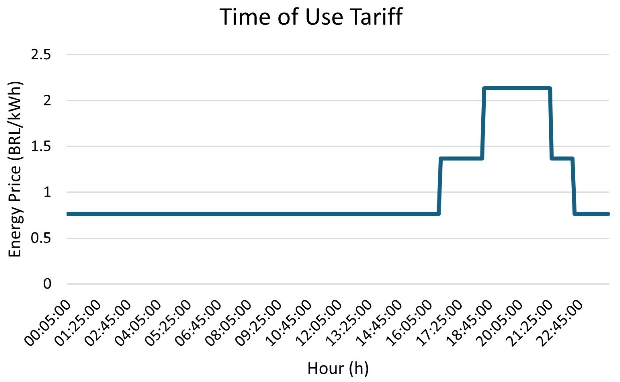
The maximum power requested and supplied to the grid ($P_{\mathrm{grid}}^{\max ,j}$) is constrained as a tool to prevent the overload of the distribution transformer at any time instant j. This restriction can be fixed or variable in time to limit energy purchases in periods of higher tariffs, depending on the tariff structure present. In this case, a fixed value is considered, since the ToU adopted for this case study bills only for the amount of energy used and not the power. Furthermore, a binary power exchange logic is formulated to prohibit the scenario of energy purchase and its injection at the same instant in time j, according to Equations (13) and (14).

$$P_{\mathrm{grid}}^{B,j}\le {\mu }_{\mathrm{grid}}^j·P_{\mathrm{grid}}^{max,j},j=k,\dots ,J$$

(13)

$$P_{\mathrm{grid}}^{I,j}\le \left(1-{\mu }_{\mathrm{grid}}^j\right)·P_{\mathrm{grid}}^{max,j},j=k,\dots ,J$$

(14)

where ${\mu }_{\mathrm{grid}}^j\in \left\{0,1\right\}$ is a binary auxiliary parameter used to indicate whether energy should be purchased or injected into the grid, according to Equation (15).

$${\mu }_{\mathrm{grid}}^j=\left\{\begin{array}{cc}1,\hfill & \mathrm{if}\mathrm{the}\mathrm{energy}\mathrm{is}\mathrm{bought},\hfill \\ 0,\hfill & \mathrm{if}\mathrm{the}\mathrm{energy}\mathrm{is}\mathrm{injected}.\hfill \end{array}\right.$$

(15)

The BESS can be charged, discharged, or remain inactive at each time step. Thus, BESS scheduling is decomposed into two variables, one for charging ($C_{\mathrm{BSS}}^j$) and one for discharging ($D_{\mathrm{BSS}}^j$), for $j=1,\dots ,J$. Both discharging/charging powers are controllable and constrained by their upper limits, i.e., $P_{\mathrm{BSS}}^{C,\mathrm{m}á\mathrm{x}}$ and $P_{\mathrm{BSS}}^{D,\mathrm{m}á\mathrm{x}}$, respectively, according to Equations (16) and (17). The power exchange logic is implemented to make it impossible to charge and discharge simultaneously, and takes the form of Equation (18).

$$C_{\mathrm{BSS}}^j·P_{\mathrm{BSS}}^{C,max}\le {\alpha }_{\mathrm{BSS}}^j·P_{\mathrm{BSS}}^{C,max},j=1,\dots ,J$$

(16)

$$D_{\mathrm{BSS}}^j·P_{\mathrm{BSS}}^{C,max}\le \left(1-{\alpha }_{\mathrm{BSS}}^j\right)·P_{\mathrm{BSS}}^{D,max},j=1,\dots ,J$$

(17)

where ${\alpha }_{\mathrm{B}\mathrm{S}\mathrm{S}}^j\in \left\{0,1\right\}$ is a binary auxiliary parameter used to indicate when the BESS is charged or discharged, according to Equation (18).

$${\alpha }_{\mathrm{BSS}}^j=\left\{\begin{array}{cc}1,\hfill & \mathrm{if}\mathrm{the}\mathrm{BSS}\mathrm{is}\mathrm{charged},\hfill \\ 0,\hfill & \mathrm{if}\mathrm{the}\mathrm{BSS}\mathrm{is}\mathrm{discharged}.\hfill \end{array}\right.$$

(18)

At the beginning of each day, the initial BESS SoC $\left(S_{\mathrm{B}\mathrm{S}\mathrm{S}}^i\right)$ is computed according to Equation (19).

$$S_{\mathrm{BSS}}^j=S_{\mathrm{BSS}}^i,\mathrm{if}j=1$$

(19)

As a guarantee that there will always be an amount of power remaining in the BESS, to maintain the system’s operation offline and provide emergency recharges, in the problem the initial SoC, $S_{\mathrm{BSS}}^i$, is set to at least 50%. Likewise, at the end of the simulation day, the final SoC is required to be at least equal to 50%, i.e., $S_{\mathrm{BSS}}^j\ge 50\%\mathrm{or}0.5,\mathrm{if}j=288$.

According to Equation (20), the BESS SoC at the beginning of the day should always be equal to or greater than the initial $S_{\mathrm{BSS}}^i$. Thus, 288 is the total j periods in a day, and $TDP$ is the total days in the chosen period (7 in a week, 30 in a month, and 365 in a year). Obviously, for simulations of only one day, this restriction can be disregarded or the value of $TDP$ can be set to 1.

$$S_{\mathrm{BSS}}^j\ge S_{\mathrm{BSS}}^i,\mathrm{if}j=288·n,n=1,\dots ,\mathrm{TDP}$$

(20)

The current SoC ($S_{\mathrm{BSS}}^j$) at any time instant j, denoted by Equation (21), can be obtained by considering the following:

• The SoC at the previous time step ($S_{\mathrm{BSS}}^{j-1}$);
• The increase in the SoC as a result of charging;
• The SoC’s decrease due to discharging.

$$S_{\mathrm{BSS}}^j=S_{\mathrm{BSS}}^{j-1}+{\displaystyle \frac{{\eta }_{\mathrm{BSS}}·P_{\mathrm{BSS}}^{C,max}·C_{\mathrm{BSS}}^j·\mathrm{Ts}}{B_{\mathrm{BSS}}}}-{\displaystyle \frac{P_{\mathrm{BSS}}^{D,max}·D_{\mathrm{BSS}}^j·\mathrm{Ts}}{{\eta }_{\mathrm{BSS}}·B_{\mathrm{BSS}}}},j=1,\dots ,J$$

(21)

where $\eta$ is the discharge/charge efficiency; $B_{\mathrm{BSS}}$ is the battery’s capacity, in kWh; and $T_s$ is the time sample, in hours. The SoC is restricted at its extreme limits to prevent overcharging and deep discharging by use of Equation (22).

$$S_{\mathrm{BSS}}^{min}\le S_{\mathrm{BSS}}^{j-1}+{\displaystyle \frac{{\eta }_{\mathrm{BSS}}·P_{\mathrm{BSS}}^{C,max}·C_{\mathrm{BSS}}^j·\mathrm{Ts}}{B_{\mathrm{BSS}}}}-{\displaystyle \frac{P_{\mathrm{BSS}}^{D,max}·D_{\mathrm{BSS}}^j·\mathrm{Ts}}{{\eta }_{\mathrm{BSS}}·B_{\mathrm{BSS}}}}\le S_{\mathrm{BSS}}^{max},j=1,\dots ,J$$

(22)

As the BESS serves as a power source in the MG, it must contain a minimum amount of energy to provide power to EVs. To guarantee this minimum requirement for the next day, the BESS’s SoC must satisfy a minimum threshold at the last time step of the current day’s scheduling, which is determined according to Equation (23).

$$S_{\mathrm{BSS}}^j+\sum _{j=k}^J\left({\displaystyle \frac{{\eta }_{\mathrm{BSS}}·P_{\mathrm{BSS}}^{C,max}·C_{\mathrm{BSS}}^j·\mathrm{Ts}}{B_{\mathrm{BSS}}}}-{\displaystyle \frac{P_{\mathrm{BSS}}^{D,max}·D_{\mathrm{BSS}}^j·\mathrm{Ts}}{{\eta }_{\mathrm{BSS}}·B_{\mathrm{BSS}}}}\right)\ge S_{\mathrm{BSS}}^{min}$$

(23)

Another restriction that can be used refers to the maximum number of charge and discharge cycles that the BESS can complete during the period considered. In this way, it is possible to reduce the loss of the capacity of the BESS due to the wear of the system caused by excess cycles, as calculated in Equations (24) and (25).

$$\sum _{j=k}^J\left(C_{\mathrm{BSS}}^j·P_{\mathrm{BSS}}^{C,max}·{\displaystyle \frac{\mathrm{Ts}}{B_{\mathrm{BSS}}}}\right)\le TCC$$

(24)

where $TCC$ is the maximum total number of charging cycles.

$$\sum _{j=k}^J\left(D_{\mathrm{BSS}}^j·P_{\mathrm{BSS}}^{D,max}·{\displaystyle \frac{\mathrm{Ts}}{B_{\mathrm{BSS}}}}\right)\le TDC$$

(25)

where $TDC$ is the maximum total number of discharge cycles. These parameters can be useful when considering periods longer than 1 day of simulation. Thus, the operation of the BESS can be limited to a maximum number of charge and discharge cycles, defined by the owner of the MG.

To ensure efficient operation and preserve the life of the BESS, restrictions have been imposed that prevent abrupt changes between its loading and discharging states. These restrictions ensure that the BESS goes through a transition state, called idling, in which it performs neither loading nor unloading, before switching between these two modes of operation.

The first constraint prevents the BESS from switching directly from its discharging mode to its charging mode. In this case, if the system was discharging in the previous period ($D^{j-1}>0$), it cannot enter charging mode in the current period ($C^j$), and it is ensured that the charging state is zero ($C^j=0$). The constraint can be mathematically expressed as in Equation (26).

$$C^j=\left\{\begin{array}{cc}0,\hfill & \mathrm{if}{D}^{j-1}>0,\hfill \\ C^j,\hfill & \mathrm{else}.\hfill \end{array}\right.$$

(26)

Similarly, the second constraint prevents the BESS from switching directly from its charging mode to its discharging mode. Thus, if the system was charging in the previous period ($C^{j-1}>0$), it cannot enter discharging mode in the current period ($D^j$), and it is ensured that the discharging state is zero ($D^j=0$). This relationship is mathematically represented in Equation (27).

$$D^j=\left\{\begin{array}{cc}0,\hfill & \mathrm{if}{C}^{j-1}>0,\hfill \\ D^j,\hfill & \mathrm{else}.\hfill \end{array}\right.$$

(27)

These restrictions ensure that the BESS operates in a stable manner, avoiding behavior that could cause premature wear and damage to the system. In addition, this approach promotes a more controlled transition between operating modes, contributing to the reliability and efficiency of the system.

In addition to technical and operational constraints, other constraints may also be included in the model. Some restrictions defined by the authors are presented below to better personalize this study.

Restriction 1: This restriction ensures that the BESS will be charged only when there are no recharges in progress in the system. The inequality in Equation (28) limits a surplus of DERs being used to charge the BESS, ensuring that this process occurs only in the absence of other recharges. This restriction prevents excessive energy being demanded from the grid at any one time.

$$\left(C_{\mathrm{BSS}}^j·P_{\mathrm{BSS}}^{C,\max }·P_{\mathrm{EVFCS}}^j\right)-\left(P_{\mathrm{PV}}^j+P_{\mathrm{W}}^j\right)\le 0,j=1,\dots ,J$$

(28)

Restriction 2: This restriction imposes a limit on the charge of the energy storage battery (BESS), ensuring that it does not exceed the instantaneous sum of the power generated by the wind and photovoltaic systems at the instant j. This condition is necessary to ensure that BESS charging only uses the energy available from the DERs, avoiding the use of external sources or the violation of the physical limits of the system, as Equation (29) denotes.

$${\mathrm{Charge}}^j\le \left(P_{\mathrm{PV}}^j+P_{\mathrm{W}}^j\right),j=1,\dots ,J$$

(29)

Restriction 3: This restriction states that the discharge power of the BESS may not exceed the maximum charging power requested by electric vehicles at the instant j. This limitation ensures that the BESS discharges only the energy necessary to meet instantaneous demand, avoiding overloading or wasting energy, while keeping the system compliant with operational requirements, as shown in Equation (30).

$${\mathrm{Discharge}}^j\le P_{\mathrm{EVFCS}}^j,j=1,\dots ,J$$

(30)

Restriction 4: This restriction limits the maximum power that can be injected into the electricity grid, ensuring that this power does not exceed the sum of the distributed generation from wind and photovoltaic sources at the instant j. This formulation allows for dynamically controlling the power injected into the grid, ensuring that the injection is limited or allowed according to the availability of distributed generation, as shown in Equation (31).

$$P_{\mathrm{grid}}^{I,j}\le \left(1-{\mu }_{\mathrm{grid}}^j\right)·\left(P_{\mathrm{PV}}^j+P_{\mathrm{W}}^j\right),j=1,\dots ,J$$

(31)

Restriction 5: This restriction ensures that at least 80% of the energy generated by DERs (wind and photovoltaic) is consumed locally, limiting the injection of energy into the electricity grid to a maximum of 20% of the total generated, as shown in Equation (32).

$$\sum _{j=k}^J\left(P_{\mathrm{grid}}^{I,j}\right)\le 20\%·\sum _{j=k}^J\left(P_{\mathrm{PV}}^j+P_{\mathrm{W}}^j\right),j=1,\dots ,J$$

(32)

This restriction promotes the efficient use of locally generated energy, reducing dependence on the power grid and minimizing losses related to the transmission and distribution of energy. In addition, it is aligned with sustainable practices and incentives about the self-consumption of renewable energy.

4. Case Study: The Application of an EMS to Manage an MG

4.1. The Definition and Characterization of the Case Study

The MG system comprises a 30 kVA (24 kW) wind turbine, a 10 kWp photovoltaic carport, an EV fast charger capable of simultaneously charging two vehicles (DC charging up to 60 kW and AC charging up to 44 kW), a BESS with a storage capacity of 215 kWh and a power capacity of up to 100 kW, and a 112.5 kVA power transformer that connects the MG to the local grid.

Figure 7 illustrates the MG used in this study and the highway layout designated to host the FCS, with one station planned approximately every 100 km [46]. The focus is on the municipality of Osório, RS, where an MG is already operational. This highway forms part of an electricity corridor strategically designed to connect Brazil and Uruguay, earning it the name the Mercosur Route.

The power generation conditions in the MG area are highly favorable, with an average wind speed of 4.62 m/s and solar radiation of 4.35 kWh/m²/day. Additionally, the highway experiences significant traffic, with an average daily flow of approximately 23,000 vehicles. This highway serves not only as the main route to the northern coast of the state but also as the connection point between the Brazilian states of Rio Grande do Sul (RS) and Santa Catarina (SC) [47].

The energy tariff considered in this study is the White ToU modality of the utility Equatorial Energia, which is for commercial consumers [48]. This tariff has different values throughout the day, with three price levels used (off-peak, intermediate, and peak hours). Figure 8 illustrates the variation in the value of the tariff throughout the hours of the day, while

Table 2. ToU tariff of the Equatorial Energia utility.

Time Period	Description	Commercial Rate (BRL/kWh)
Peak Hours	From 6:30 p.m. to 9:29 p.m.	2.13181
Intermediate Hours	From 4:30 p.m. to 6:29 p.m. and from 9:30 p.m. to 10:29 p.m.	1.36725
Off-Peak Hours	From 10:30 p.m. to 4:29 p.m. and weekends and national holidays	0.76227

Source: adapted from [48].

shows the tariff values in BRL/kWh, segmented by time range.

The MG’s has some characteristics or pre-definitions that are important to note:

• The EVFCS is self-service, that is, there are no operators. The driver must handle the equipment and recharge their EV.
• In the EMS algorithm, no type of power limiter is inserted into the charger, since the user must have their demand met in the shortest possible time. Thus, this type of option/restriction does not even appear in the EMS’s optimization.
• The minimum energy reserve in the BESS is to ensure its operation in off-grid mode, which is not addressed in this work. In this way, even with a power outage at the utility, it is still possible to guarantee some recharges and allow drivers to continue traveling.
• Some constraints are applied, such as keeping a minimum SoC of at least 50% at the end of the day and at least 30% during daily operation. This avoids deep discharge, which would damage the BESS’s lifetime, and maintains a minimum stored energy capacity to ensure a maximum of two charges in the event of a power failure or off-grid operation.
• The MG can operate in an on-grid online mode, on-grid offline mode (with the operation of the BESS in pre-defined and fixed time windows), and off-grid. In this work, the operation of the MG is addressed only in terms of its on-grid online mode, with communication via the internet achieved by local computers within the MG.
• Operation, generally, starts with a BESS SoC of at least 50% (≈108 kWh).
• The simulation runs in 5 min intervals (i.e., $T_s$ = 0.0833 h), so a day has 288 time steps (5 min intervals).
• The efficiency of energy conversion during BESS charges and discharges is 95%.
• A Net Metering discount, $D_{Net\_Met}$, of 30% of the B wire is considered, which was the value in force for 2024. The change in the energy compensation system in Brazil, brought about by Law 14,300/2022, changed the net metering model [49]. Before, the energy credits generated and consumed had an equivalence of 1 to 1, with no additional costs. As of 2023, DERs began to pay for the use of the distribution network (Wire B), which represents, on average, 28% of the final tariff. This cost will be implemented gradually: with 15% added each year, until it reaches 90% of Wire B in 2028. In 2029, the value will be revised, considering the benefits of photovoltaic energy in Brazil.
• The data acquisition, filtering, and processing routines (to estimate the EVFCS recharge curve and the DER generation curves) are performed on a local computer. Locally, the EMS algorithm, modeled in the AMPL language, is executed in a Python environment with the AMPL Python API, called amplpy, which is an interface that allows developers to access the features of AMPL from within Python version 0.13.3, which is free and has free solvers, such as the solvers HiGHS and/or SCIP [50]. Communication between the local computer and MG is achieved via the internet [51]. In the MG, an industrial computer receives the dispatch information and sends it to the PLC, which establishes the BESS dispatch set points.

The BESS used in the MG comprises lithium iron phosphate battery (LiFePO₄) modules. This technology generates the ACC vs. DoD curve shown in Figure 9.

By applying Equation (8), considering the cost of the BESS to be either BRL 1.5 million, 1.25 million, or 1 million, with a capacity of 215 kWh, the cost density curve as a function of the SoC is as presented in Figure 10.

This curve of the wear density function, $w_n\left(s\right)$, has an average cost value, ${\overline{w}}_n$, of 1.14 BRL/kWh. Considering a reduction of the cost of the BESS to BRL 1.0 million, the $w_n\left(s\right)$ has an average cost value, ${\overline{w}}_n$, of 0.7651 BRL/kWh. As this curve is nonlinear, the wear of the BESS is modeled as a piecewise linear function of the SoC, denoted by $S^j$ for each time period j. The wear, represented by $w_n^j\left(s\right)$, is defined as a function of $S^j$, and the linearization is divided into three distinct intervals, each with a specific equation that approximates the wear behavior.

Considering a BESS cost of BRL 1.5 M, which was the price paid, for each $j\in J$, the wear $w_n^j\left(s\right)$ is determined by Equation (33):

$$w_n^j\left(s\right)=\left\{\begin{array}{cc}-1.1263·S^j+1.4151,\hfill & \mathrm{if}0\le S^j\le 0.85,\hfill \\ 0.7698·S^j-0.1104,\hfill & \mathrm{if}0.85<S^j\le 0.95,\hfill \\ 20.321·S^j-18.764,\hfill & \mathrm{if}0.95<S^j\le 0.99.\hfill \end{array}\right.$$

(33)

The description of SoC ranges is as follows:

• For $0\le S^j\le 0.85$, the wear is modeled by the linear equation $-1.1263·S^j+1.4151$, which represents the wear behavior of the BESS at lower SoC levels.
• For $0.85<S^j\le 0.95$, the wear is approximated by $0.7698·S^j-0.1104$, corresponding to an intermediate SoC range.
• For $0.95<S^j\le 0.99$, the wear increases significantly and is modeled by $20.321·S^j-18.764$, reflecting higher degradation at near-full SoC levels.

The upper limit of $S^j=0.99$ was adopted because if the value obtained through the equation $w_n^j\left(s\right)$, i.e., Equation (8), is used for $S^j>0.99$, the resulting wear becomes excessively high and does not realistically represent the actual degradation of the BESS. This limitation ensures that the model remains consistent with practical observations and avoids overestimating the wear at near-full SoC levels.

4.2. Simulations and Results

Considering the variety of scenarios possible, this work presents a selected set of cases to exemplify and validate the proposed methodology. These scenarios were defined in order to encompass representative conditions of the context studied, allowing for the assessment of the applicability and efficiency of the developed approach.

4.2.1. Case I: The Average EVFCS Load

The simulations presented below consider the estimated PVS and WT generation profiles illustrated in Figure 11. It is important to note that these generation curves will vary daily and should be updated accordingly to reflect the specific conditions of each day.

In these case studies, we will present the optimization results obtained using the high-performance software for linear optimization (HiGHS) solver, which considers the problem to be a MILP model and employs the average wear cost of a BESS dispatch. Additionally, we will showcase the results produced by the Sparse Nonlinear OPTimizer (Snopt) solver in the Neos Server environment [52]. It is important to note that Snopt is a commercial solver whose full use requires a license. For Snopt, the wear density of the BESS is linearized, as described in Equation (33). However, the multiplication of two variables makes the optimization nonlinear, thereby transforming it into a Mixed-Integer Nonlinear Programming (MINLP) problem.

Historical data on arrivals at the MG reveal a consistent pattern in user behavior, with a higher demand for recharges observed at the end of the day, particularly to complete trips. It is common for users to start their journeys in the morning with fully charged batteries, while recharges become necessary later in the day to finalize planned routes. The histogram presented in Figure 12 clearly reflects this trend, indicating that the recharge demand is mainly concentrated in the mid-to-late afternoon and at night.

Then, in the first simulation, the average load curve for the MG was utilized. This curve was derived by averaging the results of 1000 simulated charging scenarios, providing a representative profile for the analysis. The resulting curve is illustrated in Figure 13.

The results obtained are summarized in

Table 3. Summary of BESS dispatches considering the average curve of EV recharges in the MG.

Variables	HiGHS Solver, ${\overline{\mathit{w}}}_{\mathit{n}}$	Snopt Solver, ${\mathit{w}}_{\mathit{n}}^{\mathit{j}}\left(\mathit{s}\right)$
Energy Charged (kWh)	0	10.79
Energy Discharged (kWh)	0	9.745
$\Delta$SoC (%)	0	5
Energy Bought (kWh)	218	209.22
Energy Sold (kWh)	25.48	14.67
Energy EVFCS (kWh)	433.64	433.64
Total WT + PVS (kWh)	240.15	240.15
OF (BRL)	290.75	295.55

Source: elaborated by the authors.

. It can be observed that using the BESS was not advantageous as it remained in standby mode. The surplus energy from DG was injected into the grid during the morning. For the remainder of the day, when local generation was insufficient to meet demand, the additional energy required was purchased from the utility grid. Although the results from the solvers show slight differences, it can be concluded that, in this scenario, using the BESS would not be economically viable. This is also supported by the fact that the total energy consumed is sufficient to ensure a self-consumption rate of more than 80% of the DG.

4.2.2. Case II: Operation on a Weekday

In the second case, the BESS dispatch for a typical weekday is considered, following the charging curve shown in Figure 14. The results are summarized in

Table 4. Summary of BESS dispatches considering a weekday charging curve.

Variables	HiGHS Solver, ${\overline{\mathit{w}}}_{\mathit{n}}$	Snopt Solver, ${\mathit{w}}_{\mathit{n}}^{\mathit{j}}\left(\mathit{s}\right)$
Energy Charged (kWh)	139.75	140.33
Energy Discharged (kWh)	126.58	85.92
$\Delta$SoC (%)	52	44.00
Energy Bought (kWh)	171.56	212.33
Energy Sold (kWh)	48.03	48.03
Energy EVFCS (kWh)	350	350.00
Total WT + PVS (kWh)	240.15	240.15
OF (BRL)	441.28	369.12

Source: elaborated by the authors.

.

In this case, the BESS is heavily utilized during peak and intermediate hours, which reduces overall costs by avoiding energy purchases during the most expensive periods. Figure 15 illustrates the usage of the BESS throughout the day. It can be observed that during periods without charging events, the BESS recharges using local DG, optimizing the MG’s self-consumption. The BESS then dispatches energy during charging periods in which the energy tariff is elevated.

Table 4 summarizes the dispatch results for this case, considering how the problem solved using the HiGHS solver, which employs the average wear cost, and the Snopt solver, where the BESS wear curve is linearized. The results indicate a tendency for the BESS to recharge throughout the day and dispatch energy within the MG during peak tariff hours. The solution obtained via Snopt proved to be more cost-effective, reducing expenses associated with excessive charging and discharging cycles.

When the BESS’s wear is based on $w_n^j\left(s\right)$, it becomes more advantageous to cycle dispatches within the SoC range of 70% to 90%, as this region exhibits lower associated wear costs. Using average wear cost values, ${\overline{w}}_n$, is advantageous, as it enables the use of free solvers such as HiGHS and SCIP. However, this approach may hinder the optimization process in terms of targeting cycling regions with lower wear costs.

Considering different BESS costs of the simulated cases, as shown by the curves in Figure 10, the most significant impact observed is in the reduction in OF costs. This is because a lower BESS cost directly reduces its degradation cost.

Table 5. Summary of BESS dispatches considering 3 different BESS costs.

Case	BESS 1.5 M	BESS 1.25 M	BESS 1.0 M
EVFCS avg load curve, OF	290.75	288.95	285.01
Weekday, OF	441.28	392.29	341.25

Source: elaborated by the authors.

presents the differences found in these cases. It is worth noting that the dispatch strategy remained practically unchanged. For the average EVFCS curve, reducing the cost of the BESS resulted in a small charge of the BESS in the morning (9.67 kWh) and a discharge (9.67 kWh) during the peak tariff period. Thus, the SoC variation during the day was only 5%. In the second case, which considers a weekday, the BESS dispatches remained almost unchanged, independent of the cost of the BESS. However, the reduction in its cost led to a more economical operation in general.

Table 6. Simulation of BESS dispatches on a weekday, without considering $w_n^j\left(s\right)$.

Variables	HiGHS Solver Without ${\mathit{w}}_{\mathit{n}}^{\mathit{j}}\left(\mathit{s}\right)$
Energy Charged (kWh)	183.08
Energy Discharged (kWh)	164.5
$\Delta$SoC (%)	55
Energy Bought (kWh)	133.64
Energy Sold (kWh)	5.05
Energy EVFCS (kWh)	350
Total WT + PVS (kWh)	240.15
OF (BRL)	102.57

Source: elaborated by the authors.

summarizes the results of the dispatch of the MG on a typical weekday, excluding the consideration of $w_n^j\left(s\right)$ and focusing solely on operational optimization without accounting for the BESS wear density function. This approach analyzes the performance of the MG’s dispatch under standard conditions, emphasizing energy balancing and cost minimization while disregarding the impact of battery degradation.

Disregarding the wear-related costs of the BESS leads to its excessive utilization, potentially accelerating its degradation and reducing the overall lifespan of the system. This is reflected in a 31% increase in the energy charged to the BESS and a 30% increase in the energy discharged. While this strategy enhances the self-consumption of the MG by maximizing the use of locally generated energy, it introduces unnecessary charge–discharge cycles.

These redundant cycles can significantly shorten the BESS’s operational lifespan by accelerating degradation. Furthermore, additional wear does not yield proportional economic benefits, as increased cycling does not generate sufficient returns to offset the reduced longevity of the BESS. As a result, this approach, although beneficial for immediate self-consumption rates, may prove unsustainable in the long term, emphasizing the importance of incorporating wear costs into the dispatch optimization process.

Other possible scenarios, such as simulations without charging events but with DG, can render the problem unsolvable. This is because the algorithm cannot satisfy its self-consumption constraints under these conditions.

In such cases, by removing the self-consumption restrictions, all the energy generated would be injected into the power grid. This decision is justified because the current period’s BESS wear cost exceeds the financial benefit provided by the net metering discount. Consequently, the system prioritizes injecting surplus energy into the grid over utilizing the BESS, which would incur higher costs without corresponding economic returns.

For scenarios involving consumption by the EVFCS and an absence of DG, the BESS tends to remain in standby mode, with all required energy purchased from the local grid. Depending on the amount of energy demanded, if the BESS has sufficient stored energy and its operational limits are respected, the algorithm may opt to dispatch the BESS during periods of elevated tariffs. This strategy seeks to reduce overall costs by leveraging stored energy to offset high energy prices.

4.2.3. Case III: A Day with Pre-Scheduled Dispatches vs. Dispatches via the Proposed Algorithm

To further exemplify and assess the performance of the proposed algorithm in greater depth, this study analyzes the differences in the operation of the MG on a typical day under two distinct approaches: a manually defined schedule set by the user and the optimized dispatch recommended by the algorithm. This comparison enables the quantification of the impacts of the optimization strategy on energy resource allocation, operational cost reduction, and the mitigation of energy storage system degradation. Moreover, the analysis highlights the importance of dynamic and intelligent energy management, demonstrating how the application of the algorithm can not only enhance the short-term operational efficiency of the MG but also significantly contribute to the longevity of system components, particularly batteries, ensuring a more sustainable and economically viable management approach over time.

To evaluate the performance of the proposed energy management algorithm under real operating conditions, this study analyzes the MG on a representative day: 22 June 2024. This day saw specific meteorological conditions that impacted distributed generation, which were characterized by an absence of sufficiently strong winds to initiate wind power generation but with favorable solar radiation by winter standards. The initial SoC of the BESS was considered based on the last recorded value from previous operations, reflecting the continuous nature of the MG’s operational cycle. Our analysis compares two energy dispatch approaches throughout this day: a manually defined schedule set by the user and the optimized strategy recommended by the algorithm. This comparison allows for quantifying efficiency gains, reductions in operational costs, and the impact on battery degradation, demonstrating the relevance of intelligent control in maximizing the utilization of renewable energy and extending the lifespan of the storage system.

Figure 16 and Figure 17 represent the DG for the day analyzed and the EV charging events, respectively. These figures provide a clear visualization of the availability of renewable energy sources and the corresponding charging demand, serving as fundamental elements in assessing the effectiveness of the proposed energy management strategy.

Initially, the dispatch was carried out according to a manually set schedule defined by the user, without any forecasting or energy management strategy. In this case, throughout the day, the BESS operated its dispatch as shown in Figure 18, with its SoC varying over time as illustrated in Figure 19. This scenario serves as a baseline for comparison, highlighting the differences in performance and efficiency when the optimized strategy is applied.

In this manually scheduled dispatch scheme, there is no consideration for energy prices, DG availability, or energy management strategies aimed at cost reduction. As shown, the BESS fluctuates throughout the day, dropping to 40% SoC and reaching up to 88%, without prioritizing local DG utilization. A significant amount of energy is purchased from the grid, disregarding price variations, while BESS cycling occurs without optimization, leading to increased wear and reduced efficiency. This highlights the drawbacks of an unoptimized dispatch strategy, reinforcing the need for an intelligent EMS to enhance cost-effectiveness and system longevity. By repeating the study for the same day but applying the proposed methodology, a different dispatch pattern is observed.

Next, the EMS evaluation of the case and its decision-making process for BESS operation are presented. Figure 20 illustrates the optimized BESS dispatches, while Figure 21 depicts its SoC variation throughout the day. Additionally, Figure 22 shows the energy exchanges with the utility grid during the MG’s operation. These results highlight the EMS’s ability to optimize resource utilization, minimize costs, and improve overall system efficiency compared to the manually scheduled dispatch.

The optimization of energy management in the analyzed MG demonstrated improvements in operational efficiency, cost savings, and the preservation of the BESS’s lifespan. The proposed strategy focused on minimizing operational costs by optimizing the decision-making process regarding whether to store or utilize energy.

The results indicate a significant reduction in the charging and discharging cycles of the BESS, with only 5.75 kWh charged and 6.00 kWh discharged throughout the day, leading to a mere 2% variation in its SoC. This dispatch strategy contrasted sharply with that of conventional operation, where the BESS underwent deep charge–discharge cycles, directly impacting its degradation. Minimizing the amplitude of these cycles contributes to extending its battery life, thereby reducing long-term replacement and maintenance costs.

From an energy balance perspective, the total energy purchased from the grid amounted to 238.46 kWh, while 2.89 kWh was injected back into the grid. The total energy allocated for EV charging reached 263.05 kWh, with local DG contributing 28.02 kWh. This distribution indicates that although the MG still relies significantly on the power grid, optimization enabled better utilization of the available renewable generation, reducing the need for energy purchases during peak tariff periods.

An important aspect to highlight is that under scheduled dispatches, the BESS was charged during non-charging periods and subsequently discharged during charging periods. However, this approach only resulted in additional BESS cycles without yielding significant economic benefits. This behavior underscores the importance of an optimization model that considers not only charge and discharge scheduling but also its economic impact and battery degradation reduction.

The final OF value obtained after optimization was BRL 219.74, reflecting a substantial reduction in operational costs compared to non-optimized operation. This cost reduction is primarily attributed to intelligent BESS management, which prevented unnecessary discharges and prioritized energy storage during strategic periods. The daily tariff curve further emphasizes the significance of this control, as the adopted strategy minimized energy purchases during high-cost periods.

Thus, the results demonstrate the feasibility and effectiveness of the proposed optimization model. This approach not only reduces operational costs but also ensures the more sustainable use of energy resources, enhances the integration of renewable sources, and increases MG resilience. Moreover, minimizing BESS degradation reinforces the importance of optimization strategies aimed at extending the lifespan of energy storage systems, a crucial factor in the economic and environmental viability of distributed energy infrastructures.

4.3. Discussion

In these examples, the operation of the MG was only considered within a one-day period. However, the methodology is flexible and can be applied to longer periods. In the optimization model, you should adjust the size of the J set and ensure the input data are the same size. In case of optimizations for months or years, historical average data for EV charging curves and DER generations can be used as an alternative, since short-term forecasts do not apply over these periods.

Other strategies have addressed similar problems. For instance, ref. [54] proposed managing FCSs using dynamic programming. However, that study considered only PVS generation and batteries, neglecting any costs related to battery degradation caused by the operation. The primary objective was to minimize power transfer at the point of common coupling (PCC) while also accounting for energy pricing.

Similarly, ref. [55] addressed energy management in an isolated MG. While the presented results are satisfactory, the methodology also overlooks the degradation costs of the BESS. Furthermore, the use of paid tools, such as MATLAB software, version 2017b, may lead to additional costs for users, which is avoided by using open-source packages and programming languages like Python, version 3.11.5

In [56], the focus was on minimizing the charging cost of EVs, relying solely on PVS generation as the renewable source of energy. The data granularity in the study was hourly, whereas our proposal adopts a 5 min granularity to capture critical information that could be lost within hourly intervals. The referenced study also neglects the costs associated with BESS degradation.

Finally, ref. [57] proposed rule-based energy management, with DER forecasts updated every 15 min using an ANN for PVS and meteorological data for wind generation. Dispatch decisions were based on rules, ensuring technical operation and fulfilling the preferences set by the nanogrid owner. However, incorporating and modeling the costs of BESS degradation would make the study more realistic and help extend the BESS’s lifespan, avoiding premature failure caused by overuse.

The studies here highlight the importance of the management strategy applied to MGs. Furthermore, understanding, modeling, and pricing the degradation costs of BESSs enable their owner to maximize profitability, enhance the energy utilization of the MG, and extend the lifespan of the storage system.

The increasing complexity of the electrical sector, driven by regulatory changes, new tariff models, and rising energy costs, reinforces the need for advanced optimization strategies. This trend suggests that intelligent energy management solutions will become increasingly essential for consumers seeking greater economic and operational efficiency. In this context, optimized energy dispatch methodologies, such as the one proposed in this study, could be a competitive advantage for MGs, facilitating the better integration of renewable sources, cost reductions, and greater autonomy from the conventional power grid.

5. Conclusions

This study conducted a comprehensive analysis of the integration of DERs into an MG, with a specific emphasis on their interaction with a BESS. The findings highlight that DERs in MGs, particularly when supported by a BESS, represent an effective strategy to enable reliable and sustainable off-grid operation. The EMS developed in this work also demonstrated efficiency and agility, standing out for its modularity, which allows easy modifications and adaptability to various configurations.

The results indicate that the degradation of the BESS significantly affects the operational cost of an MG, as the BESS remains a high-cost component. The estimated average degradation costs are 1.14 BRL/kWh for systems valued at BRL 1.5 million and 0.766 BRL/kWh for systems valued at BRL 1 million. Consequently, in the current configuration, the BESS tends to be underutilized, as its degradation cost often exceeds the benefits provided by net metering discounts, considering current energy tariffs and discount rates. However, it was observed that the BESS is utilized in scenarios where user self-consumption constraints are imposed. These constraints, which define the minimum self-consumption levels required, drive the strategic operation of the BESS at times that minimize MG operational costs while meeting self-consumption requirements.

Future projections suggest that reducing BESS acquisition and operational costs, combined with rising energy tariffs and regulatory changes, such as total restrictions on excess energy injection into the grid or associated penalties, could enable the wider use of BESSs in the long term. Moreover, dynamic tariffs, such as peak-hour rates, have the potential to make BESS usage economically advantageous. An additional aspect identified was the energy conversion efficiency of the BESS, which, although relevant, may limit its economic attractiveness. Energy conversion losses negatively impact the competitiveness of BESSs compared to direct energy injection into the grid, for which such losses were not modeled in this study.

Based on the results obtained, several opportunities for future research have been identified. Among them is the incorporation of rule-based models to enable real-time MG operation control, allowing for the correction of deviations from planned models. Additionally, refining DER generation forecasting models and recharge estimation algorithms is suggested to be able to improve system accuracy and efficiency. Another relevant perspective is extending the MG dispatch programming horizon to weekly scales or shorter intervals, such as intra-hourly periods, to better capture the dynamic operational conditions of the system.