Planning Amidst Uncertainty: Identifying Core CCS Infrastructure Robust to Storage Uncertainty

Abstract

Carbon Capture and Storage (CCS) is a critical technology for reducing anthropogenic CO₂ emissions, but its large-scale deployment is complicated by uncertainties in geological storage performance. These uncertainties pose significant financial and operational risks, as underperforming storage sites can lead to costly infrastructure modifications, inefficient pipeline routing, and economic shortfalls. To address this challenge, we propose a novel optimization workflow that is based on mixed-integer linear programming and explicitly integrates probabilistic modeling of storage uncertainty into CCS infrastructure design. This workflow generates multiple infrastructure scenarios by sampling storage capacity distributions, optimally solving each scenario using a mixed-integer linear programming model, and aggregating results into a heatmap to identify core infrastructure components that have a low likelihood of underperforming. A risk index parameter is introduced to balance trade-offs between cost, CO₂ processing capacity, and risk of underperformance, allowing stakeholders to quantify and mitigate uncertainty in CCS planning. Applying this workflow to a CCS dataset from the US Department of Energy’s Carbon Utilization and Storage Partnership project reveals key insights into infrastructure resilience. Reducing the risk index from $15\%$ to $0\%$ is observed to lead to an $83.7\%$ reduction in CO₂ processing capacity and a $77.1\%$ decrease in project profit, quantifying the trade-off between risk tolerance and project performance. Furthermore, our results highlight critical breakpoints, where small adjustments in the risk index produce disproportionate shifts in infrastructure performance, providing actionable guidance for decision-makers. Unlike prior approaches that aimed to cheaply repair underperforming infrastructure, our workflow constructs robust CCS networks from the ground up, ensuring cost-effective infrastructure under storage uncertainty. These findings demonstrate the practical relevance of incorporating uncertainty-aware optimization into CCS planning, equipping decision-makers with a tool to make informed project planning decisions.

1. Introduction

Carbon Capture and Storage (CCS) is a critical climate change mitigation technology aimed at reducing anthropogenic CO₂ emissions from industrial processes. CCS operates by capturing CO₂ at stationary emission sources such as power plants, transporting it via networks of pipelines, and injecting it into geological reservoirs for long-term storage. Case studies in the adoption of CCS have been conducted for many regions of the world [1,2,3,4], and multiple operational projects are in progress worldwide [5]. To have a meaningful impact on global CO₂ emissions, CCS must be deployed on a massive scale, involving projects of dozens to hundreds of emission sources, thousands of kilometers of pipelines, and numerous storage sites. Deploying infrastructure on this scale requires significant planning and investment, while contending with a range of uncertainties that can impact project performance and cost [6]. One key source of uncertainty for CCS project design is the uncertainty associated with geological reservoir capacity and injectivity. Even with thorough site characterization, the true performance of a reservoir often remains unknown until injection operations are under way. If a storage site lacks the capacity for the full estimated volume of CO₂, the excess amount must either be vented or rerouted to alternate storage sites, which may themselves face similar performance uncertainties. Such scenarios can lead to costly modifications to infrastructure, increased transportation distances, and risks to the economic and operational viability of CCS projects.

In an effort to address these challenges early in the planning phase of a project, this paper introduces a novel approach to designing CCS infrastructure that explicitly accounts for storage uncertainty. This approach aims to identify core CCS infrastructure that has a high likelihood of being functional throughout the life of the project and is cost-effective to operate, even though future site-specific storage performance is not well known. Appetite for risk is incorporated into this approach to provide the ability to trade off the cost and performance of the identified infrastructure with the risk that it will require modifications during actual injection operations, when the true storage performance becomes known.

In this approach, multiple network design scenarios are generated, where each one represents a unique set of annual storage capacities for the available reservoirs, with the capacities being sampled from reservoir-specific distributions. Optimal infrastructure design solutions are computed for each scenario using the open source $SimCCS$ optimization software for CCS infrastructure design [7]. These solutions are then aggregated into a heatmap, which quantifies the frequency with which each network component (e.g., pipelines, storage sites, and source sites) appears across the multiple scenario solutions. This heatmap allows decision-makers to identify core infrastructure components that are consistently utilized across scenarios. Using the heatmap as a foundation, the workflow then enables the computation of minimum-cost maximum-flow network solutions at varying levels of risk tolerance. For example, a high-confidence solution may only include components used in nearly all scenarios, resulting in infrastructure that is very likely to remain functional when the true storage parameters become evident during injection operations. On the other hand, a more flexible solution might allow for the inclusion of less frequently used components, resulting in infrastructure with more processing capacity. However, this increase in processing capacity comes at the cost of an increased risk of underperforming during injection operations, potentially requiring modifications to achieve the originally planned CO₂ processing targets. This workflow provides stakeholders with a tool to balance cost, performance, and storage risk in large-scale deployment scenarios.

Significant research has been devoted to accurately estimating the storage performance of geological reservoirs to support reliable CCS infrastructure planning. Research has been conducted to advance site characterization and performance modeling techniques aimed at reducing uncertainties in storage reservoir behavior [8,9,10,11,12]. However, despite these advancements, significant uncertainties persist, emphasizing the need for infrastructure designs that can withstand deviations from predicted storage performance [13,14,15]. The workflow we propose in this study is designed to enable effective infrastructure planning despite persistent storage uncertainties, rather than relying on the ability to predict storage parameters with high accuracy.

Existing research has explored various strategies to address uncertainty in CCS infrastructure design, including uncertainties in economic factors such as CO₂ taxes [16] and capture technology [17]. Other efforts have focused on reducing the complexity of uncertainty modeling by narrowing the search space of geological realizations [18]. While these approaches simplify scenario generation, they do not provide a structured framework for designing infrastructure under uncertainty. In contrast, this study presents such a framework that explicitly integrates storage uncertainty into the infrastructure design process.

Numerous studies have used stochastic models to explore CCS infrastructure design under parameter uncertainty [19,20,21,22,23,24]. However, these approaches either focus on highly simplified small-scale networks or do not incorporate pipeline routing optimization, which is critical for cost-effective deployment. Since CO₂ transportation represents a major cost driver in CCS projects, neglecting pipeline routing optimization overlooks key spatial considerations, such as geographical obstacles and trunk line routing, which are essential for accurately quantifying infrastructure costs. We demonstrate in Section 4 that our proposed process optimizes source/sink selection and pipeline routing for a non-trivial dataset of 119 sources and sinks, showing its applicability to real-world CCS planning.

In [25], the authors considered designing infrastructure that is resilient when subjected to multiple failures across the CCS supply chain. Their findings highlight the trade-offs between resilience and cost, with solutions such as CO₂ trucking offering increased flexibility. However, trucking is not economically viable for transporting large volumes of CO₂ over long distances, as pipelines provide far greater cost efficiency due to economies of scale [26,27]. In contrast, our approach explicitly integrates pipeline routing optimization into the infrastructure design process, ensuring that CCS networks remain both cost-effective and resilient to storage uncertainty. By leveraging cooperative trunk lines and optimized routing, our method captures the financial advantages of large-scale pipeline deployments.

In [28], the authors proposed an approach in which multiple scenarios are optimally solved and the minimum cost to adapt each scenario to the others is calculated. While this method effectively identifies the solution that is the cheapest to modify post-deployment, it does not explicitly design infrastructure to be inherently resilient to uncertainty. Instead, it selects the most adaptable option from a limited set of predefined scenarios, without guaranteeing an optimal long-term solution. In contrast, our approach constructs infrastructure from the ground up to be inherently robust to uncertainty. Rather than selecting a solution that is simply the easiest to adjust later, our method proactively designs networks to perform reliably across a broad range of possible storage outcomes—including those not explicitly anticipated during scenario generation. This ensures that key infrastructure components are cost-effective, resilient, and less dependent on post-deployment repairs.

In [29], the authors introduced a framework that identifies infrastructure designs that minimize repair costs in the event of reservoir underperformance, balancing upfront investment with potential future modifications. While this approach focuses on minimizing repair costs, it does not necessarily prevent failures from occurring in the first place. In contrast, our method takes a proactive approach by designing infrastructure that is inherently resilient to storage uncertainty, reducing the likelihood of underperformance and the need for costly repairs altogether. By identifying robust network components during the design phase, our workflow ensures that infrastructure remains functional and cost-effective under a broad range of uncertain storage conditions.

Our proposed workflow uses a heatmap as a core component of the optimization process, rather than as a data visualization tool, as is widely practiced [30,31,32,33]. Heatmaps have been applied to uncertainty management in fields beyond infrastructure optimization, including medical image processing [34,35], automated data annotation [36], and genetic expression analysis [37]; while heatmaps have also been used in civil infrastructure studies [38,39,40], their primary role has been to visualize data or solutions rather than actively guide optimization. In contrast, our proposed workflow employs heatmaps not as a visualization tool but as an integral step in the optimization process by aggregating network structures from previous iterations and informing targeted network design in subsequent steps.

Our work presented in this paper advances the state of uncertain CCS infrastructure design by offering a systematic approach to manage storage uncertainty. The rest of this paper is organized as follows: Section 2 provides background information on CCS infrastructure modeling and parameter uncertainty. Section 3 introduces a heatmap-based optimization work flow for designing CCS infrastructure subject to storage uncertainty. Section 4 demonstrates the proposed framework using data from the US Department of Energy’s Carbon Utilization and Storage Partnership (CUSP) project, one of the DOE’s Regional Initiatives to Accelerate CCS Deployment. Finally, the paper is concluded in Section 5.

2. Background

The problem of determining optimal CCS infrastructure can be formulated as a mixed-integer linear programming (MILP) problem. Mixed-integer linear programming is a mathematical optimization approach widely used for planning and decision-making in complex systems. The goal of MILP models is to minimize or maximize an objective function, which is the algebraic representation of some parameter of interest (e.g., cost, productivity, or throughput) in the system being modeled. The objective function is encoded with data from the problem and decision variables, which are unknown elements of the problem that one wishes to determine (e.g., the amount of product to produce or the location to which a resource is to be deployed). MILPs combine continuous decision variables, which represent quantities such as flow rates, with binary decision variables, which indicate on/off decisions for components such as the construction (or not) of pipelines. An MILP solver (e.g., IBM’s CPLEX software) manipulates the decision variables in order to optimize the objective function. Linear inequality functions called constraints are used to enforce problem properties (e.g., capacity restrictions). A solution to an MILP model is represented by specific values for the decision variables and the value of the solution is the value of the objective function.

MILPs are a logical way to model CCS infrastructure design problems compared to machine learning approaches for several reasons. First, MILPs are designed to provide globally optimal solutions, which is the overarching goal of CCS infrastructure design problems where cost minimization is the primary goal. Second, CCS infrastructure design problems are highly formalized and constrained, making them well suited to mathematical optimization through an MILP. Finally, there is insufficient data available to train a machine learning model for CCS infrastructure design, as the deployment of CCS systems is still limited globally.

The goal of the optimal CCS infrastructure MILP model is to determine the minimum-cost infrastructure deployments of sufficient capacity. Since the goal is to minimize CCS infrastructure cost, the data that are fed into the MILP model are composed of the key cost drivers of a CCS project, including the following: source information (location, capture costs, and emission rate); storage information (location, injection costs, and storage capacity); and transport information (pipeline routes and pipeline cost–capacity curves). Information on the input data is presented below.

• Instance Input Data:

S	Set of CO2 sources
$Q_i^{src}$	Annual CO2 production rate at source i (MtCO2/yr)
$F_i^{src}$	Fixed cost of opening source i (USD)
$V_i^{src}$	Variable cost of capturing CO2 from source i (USD/MtCO2)
R	Set of storage sites
$Q_j^{res}$	Annual CO2 capacity of storage site j (MtCO2/yr)
$F_j^{res}$	Fixed cost of opening storage site j (USD)
$V_j^{res}$	Variable cost of injecting CO2 into storage site j (USD/MtCO2)
P	Set of candidate pipelines
C	Set of possible capacities for each pipeline
$Q_{kc}^{min}$	Minimum capacity of pipeline k with capacity c (MtCO2/yr)
$Q_{kc}^{max}$	Maximum capacity of pipeline k with capacity c (MtCO2/yr)
$F_{kc}^{pipe}$	Fixed cost of opening pipeline k with capacity c (USD)
$V_{kc}^{pipe}$	Variable cost of transporting CO2 via pipeline k with capacity c (USD/MtCO2)
J	Set of candidate pipeline junctions
T	Annual target CO2 processing amount

The decision variables of the infrastructure design MILP indicate which sources to open and how much CO₂ to capture from each, which storage locations to open and how much CO₂ to inject into each, and where to deploy pipelines and what capacity they need to be able to transport. Details on the decision variables are presented below.

• Decision Variables:

$s_i\in \{0,1\}$	Indicates whether source i is opened
$a_i\in {\mathbb{R}}^{\ge 0}$	Annual amount of CO2 captured from source i (MtCO2/yr)
$r_j\in \{0,1\}$	Indicates whether reservoir j is opened
$b_j\in {\mathbb{R}}^{\ge 0}$	Annual amount of CO2 injected into reservoir j (MtCO2/yr)
$p_{kc}\in \{0,1\}$	Indicates whether pipeline k with capacity c is opened
$d_{kc}\in {\mathbb{R}}^{\ge 0}$	Annual amount of CO2 put in pipeline k with capacity c (MtCO2/yr)

The goal of the MILP is to minimize the cost of the project. The objective function that realizes this goal quantifies the cost of the project as the sum of the cost to capture the CO₂, the cost to transport the CO₂, and the cost to store the CO₂. The cost to capture CO₂ is the cost to open each opened facility ($F_i^{src}$) plus the cost to capture each ton of CO₂ from it ($V_i^{src}{a}_i$). Similarly, the cost to store CO₂ is the cost to open each opened storage location ($F_j^{res}$) plus the cost to inject each ton of CO₂ into it ($V_j^{res}{b}_j$). The cost to transport CO₂ is the cost to build each opened pipeline ($F_{kc}^{pipe}$) plus the cost to utilize the opened pipeline ($V_{kc}^{pipe}{d}_{kc}$). Since the goal is minimum-cost infrastructure, this objective function is minimized. The objective function is presented below.

• Objective Function:

$$min\stackrel{\mathrm{capture} \mathrm{cost}}{\overbrace{\sum _{i\in S}(F_i^{src}{s}_i+V_i^{src}{a}_i)}}+\stackrel{\mathrm{transport} \mathrm{cost}}{\overbrace{\sum _{k\in P}\sum _{c\in C}(F_{kc}^{pipe}{p}_{kc}+V_{kc}^{pipe}{d}_{kc})}}+\stackrel{\mathrm{storage} \mathrm{cost}}{\overbrace{\sum _{j\in R}(F_j^{res}{r}_j+V_j^{res}{b}_j)}}$$

Constraints are used to enforce realistic operational restrictions including capacity restrictions and standard network construction requirements. The constraints are presented below.

Constraints:

$$\begin{array}{cc}\hfill & Q_{kc}^{min}{p}_{kc}\le d_{kc}\le Q_{kc}^{max}{p}_{kc},\forall k\in P,\forall c\in C\hfill \end{array}$$

(1)

$$\sum _{\begin{array}{c}k\in P:\\ src\left(k\right)=n\end{array}}\sum _{c\in C}{d}_{kc}-\sum _{\begin{array}{c}k\in P:\\ dest\left(k\right)=n\end{array}}\sum _{c\in C}{d}_{kc}=\left\{\begin{array}{cc}{a}_n\hfill & \mathrm{if}n\in S\hfill \\ -b_n\hfill & \mathrm{if}n\in R\hfill \\ 0\hfill & \mathrm{if}n\in J\hfill \end{array}\right.,\forall n\in S\cup R\cup J$$

(2)

$$\begin{array}{cc}\hfill & a_i\le Q_i^{src}{s}_i,\forall i\in S\hfill \end{array}$$

(3)

$$\begin{array}{cc}\hfill & b_j\le Q_j^{res}{r}_j,\forall j\in R\hfill \end{array}$$

(4)

$$\begin{array}{cc}\hfill & \sum _{i\in S}{a}_i\ge T\hfill \end{array}$$

(5)

where constraint (1) enforces minimum and maximum pipeline capacities by ensuring that the amount of CO₂ transported by a pipeline ($d_{kc}$) is greater than the minimum capacity ($Q_{kc}^{min}$) and less than the maximum capacity ($Q_{kc}^{max}$) of that pipeline. Constraint (2) enforces conservation of flow at each node in the network to ensure that CO₂ is only added to the network when captured from sources and only leaves the network when injected into sinks. In other words, constraint (2) ensures that all CO₂ in the network comes from a source and goes to a storage site. Constraint (3) enforces limitations on source production rates by forcing the amount of CO₂ captured at each source ($a_i$) to be less than the available amount of CO₂ at that source ($Q_i^{src}$). Constraint (4) enforces limitations on reservoir storage capacities by forcing the amount of CO₂ injected into each storage site ($b_j$) to be less than the capacity of that site ($Q_j^{res}$). Constraint (5) ensures that the total amount of CO₂ processed by the system meets the target.

Uncertainty in the CCS supply chain can be reflected in the model as uncertain values in the component costs ($F_X$ and $V_X$) or the component capacities ($Q_X$). For the purposes of this study, the uncertainty of storage capacity and injectivity is reflected in uncertain values of the annual storage capacity parameter $Q_j^{res}$. The model assumes a constant injection rate over the life of the project; thus, a decrease in total storage capacity corresponds to a decrease in the annual storage capacity $Q_j^{res}$. Likewise, a decrease in injectivity corresponds to a decrease in the annual storage capacity $Q_j^{res}$ of that site. The MILP model optimally solves problems where all of the input data are known exactly. However, the MILP model is unable to handle scenarios where there is input data uncertainty. As such, a more sophisticated workflow is needed to incorporate uncertainty into CCS infrastructure modeling. The following section introduces a workflow to tackle this limitation, leveraging probabilistic techniques to design infrastructure that remains operational and cost-effective under uncertain storage conditions.

3. Infrastructure Design Process

In this section, we introduce a heatmap-based method for identifying core CCS infrastructure that is resistant to storage capacity uncertainty. If all of the input parameters for a CCS infrastructure design instance were exactly known, optimal infrastructure solutions could be determined by solving the MILP model detailed in Section 2. However, we assume that the actual annual capacity of each storage site, $Q_j^{res}$, is uncertain and can be represented by a site-specific probability distribution. Each probability distribution is based on geologically informed estimates, reflecting the uncertainty in reservoir performance. Since the capacity of each site is not exactly known, this uncertainty prevents optimal infrastructure solutions from being determined by solving the MILP model. Instead, we propose a stochastic process for designing infrastructure that functions even with uncertain annual storage capacities.

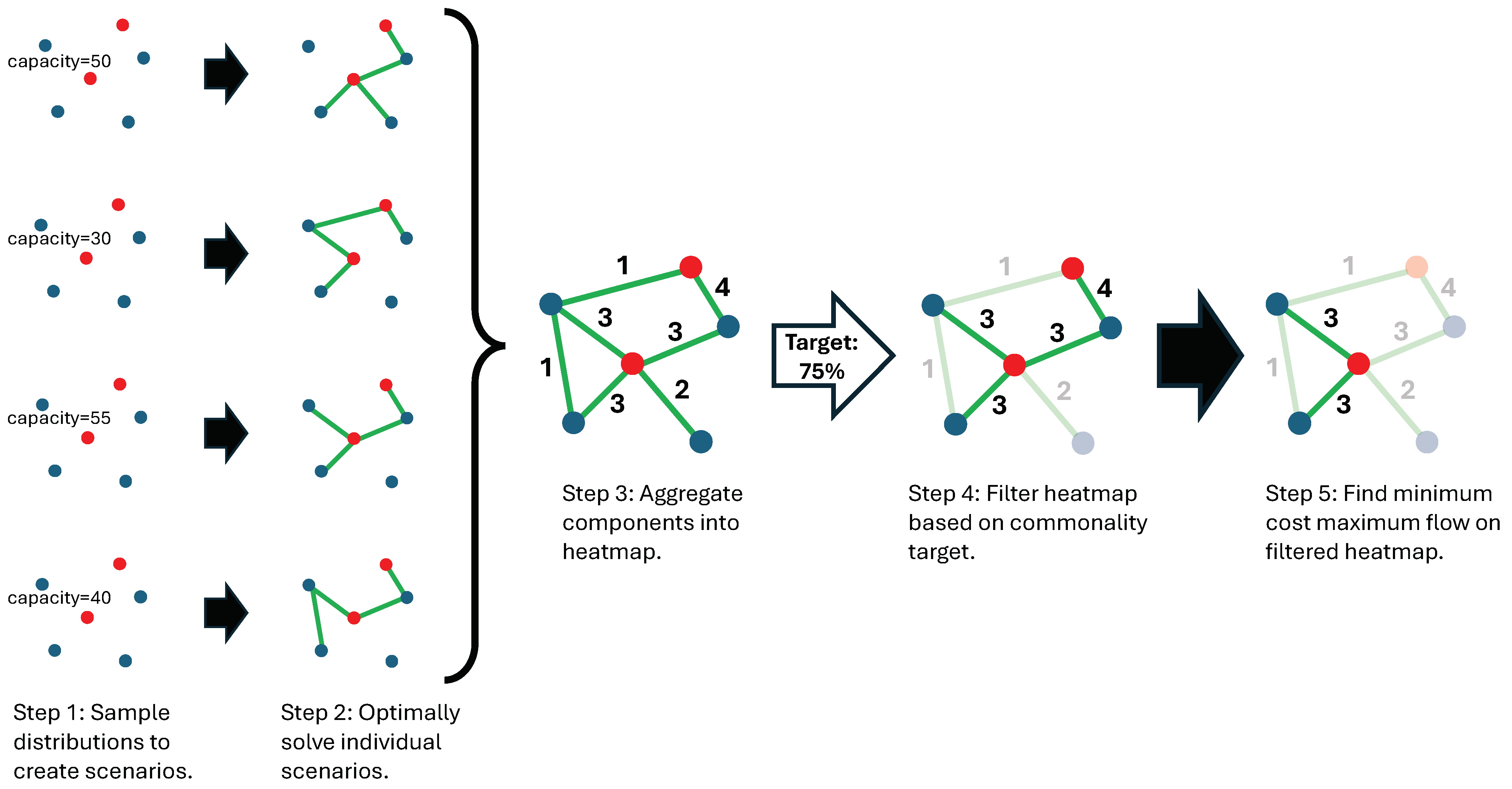
At a high level, the proposed infrastructure design process is a Monte Carlo optimization framework that first generates discrete scenarios by randomly sampling each storage site’s probability distribution. Each scenario is then solved using the MILP model detailed in Section 2 to determine the optimal infrastructure needed to support that scenario. The optimal infrastructure solutions for each scenario can then be aggregated together into a heatmap to identify infrastructure components common to multiple solutions. Next, the heatmap is filtered to only include infrastructure that is common to a specified number of solutions or more. Finally, a core infrastructure design is identified by finding the minimum-cost maximum-flow solution in the filtered heatmap. An illustration of the proposed infrastructure design process is presented in Figure 1 and detailed below.

3.1. Scenario Generation

The MILP model detailed in Section 2 requires concrete values for all input parameters, including the site-specific annual storage capacities $Q_j^{res}$. To construct a concrete scenario from uncertain storage capacities that can be solved using the MILP model, each storage site’s capacity is selected as a random value sampled from that site’s probability distribution. This process is repeated to generate a set of scenarios, where each scenario represents a unique realization of the annual storage capacities for all storage sites. This set of scenarios captures a range of potential outcomes, ensuring that, with a sufficiently large set, the infrastructure design process will likely be exposed to storage conditions similar to what will be encountered in deployment.

3.2. Scenario Optimization

Each scenario is independently optimized using the MILP model detailed in Section 2. Solving the MILP model for each scenario determines the infrastructure components needed to support that scenario, including the following:

• The set of sources to open and their associated capture rates;
• The set of storage sites to open and their associated injection rates;
• The network of pipelines to deploy and their capacities.

Solving the MILP model for each scenario yields an optimal infrastructure solution for that specific realization of storage capacities.

3.3. Heatmap Generation

The individual solutions from all scenarios are aggregated to generate a heatmap that represents the frequency with which each infrastructure component (e.g., pipeline, source, or storage site) appears across the set of scenario solutions. A commonality score is calculated for each component as the number of scenario solutions in which that component appears. The commonality score is represented as the numerical edge weights in the graph in step 3 of Figure 1. The result is higher commonality scores for infrastructure components with higher usage frequencies, which indicate greater importance and resilience across a range of uncertainty realizations. Each commonality score can be translated into a value in the range $[0,1]$, representing the percentage of scenario solutions in which the component appeared, by dividing it by the number of scenarios.

3.4. Heatmap Filtering

An abstract concept of risk mitigation is incorporated into the design process in the form of a risk index, which assumes a value of $0\%\le X\le 100\%$. This index represents two things in the workflow that manage the risk that the core CCS infrastructure found will require repair due to storage underperformance during operation with the real storage capacities. First, for a given risk index X, a network component (e.g., pipeline, source, our storage site) must have a minimum commonality score of $(100-X)$ to be included in the filtered heatmap. As the risk index decreases, the filtered heatmap retains only infrastructure that appears in a larger number of scenario solutions, effectively reducing the available infrastructure to the most common components. This results in a more conservative, lower-risk assessment of infrastructure availability. For example, at $X=0\%$, only network components that appear in the optimal solutions of all scenarios (those with a commonality score of 100) are included, offering high confidence that any of those components would remain functional during actual injection operations. At $X=15\%$, components used in at least $85\%$ of scenarios are included in the filtered heatmap, allowing more infrastructure possibilities at an increased risk of deploying infrastructure that will underperform with the actual storage capacities and require repair. All network components that appear in fewer than $X\%$ of the scenario solutions are excluded from the final infrastructure design.

3.5. Core Infrastructure

While the filtered heatmap identifies infrastructure that is common to $X\%$ of all scenarios, there is no guarantee that this infrastructure forms a valid flow solution. For example, the filtered heatmap could contain pipeline components that are not connected to any other infrastructure with the same risk index. In this case, the filtered heatmap infrastructure would not serve as a stand-alone solution. To determine the largest valid solution contained within the filtered heatmap, the minimum-cost maximum flow over that network is computed. Maximum flows represent solutions in the filtered heatmap that are able to host the largest amount of CO₂. The minimum-cost solution among the set of maximum flow solutions represents the most cost-effective maximum flow. Minimum-cost maximum flows in the filtered heatmap infrastructure can be found by iteratively solving versions of the MILP model from Section 2. First, the maximum flow is determined by performing a binary search on values of the annual CO₂ processing target T, looking for the largest threshold value that results in a feasible MILP instance. Once the maximum flow is found, the minimum-cost maximum flow is found by solving the MILP model one more time with the processing target T set to equal the maximum flow value. However, before the MILP model from Section 2 can be formulated, concrete storage capacities need to be identified from the site-specific probability distributions. This is done by again leveraging the risk index value. Given a risk index of X, the storage capacity of each site is set to the Xth percentile of the site’s probability distribution.

For example, if a decision-maker with a low appetite for risk wanted to explore possible infrastructure deployments, they might choose a risk index of $X=10\%$. In that case, only infrastructure that was deployed in at least $90\%$ of the scenario solutions would be considered. The storage capacity for all of those storage sites would be set at the very conservative 10th percentile of their probability distributions. The resulting core infrastructure found when calculating the minimum-cost maximum flow would reflect a very conservative set of assumptions, and it is very likely that this core infrastructure would perform well with whatever storage capacities are actually encountered during operation. On the other hand, if the decision-maker had a large appetite for risk, they might choose a risk index of $X=75\%$. In this case, the amount of available infrastructure would increase greatly, and the storage capacity for all of those sites would be set at the 75th percentile of their probability distributions. This would reflect a far more optimistic view and would result in core infrastructure that is larger and capable of processing significantly more CO₂ but is also at a greater risk of requiring repair due to storage site underperformance. In this way, the risk index serves as a parameter of the model that represents the appetite for risk during the infrastructure generation process. This process can also be modified to have a different storage capacity selection method (e.g., always select the expected value) should a specific case study warrant it.

3.6. Workflow Discussion

While this proposed workflow for designing CCS infrastructure provides a framework for addressing storage capacity uncertainty, there are numerous practical details that should be considered. The underlying infrastructure design optimization problem is a known NP-hard problem [41]. This means that, although solving the MILP model will produce globally optimal solutions, the computational running time will increase exponentially as the size of the dataset increases (e.g., by increasing the number of sources, storage sites, or candidate pipelines). This can pose significant scalability challenges when applying the proposed process to very large datasets, such as those representing multi-region or nationwide CCS studies. In such cases, additional computational resources or heuristic approximations may be required to maintain tractability.

Implementation of the proposed workflow is a straightforward process, since existing CCS infrastructure modeling tools such as $SimCCS$ and $CostMAP$ can be heavily leveraged [7,42]. These tools handle data organization and visualization while employing off-the-shelf MILP solvers such as CPLEX or Gurobi to solve the core MILP model. Modifications to existing software (e.g., $SimCCS$) need to be made to support the stochastic component of the workflow and to aggregate solutions into heatmaps for display.

Finally, as is true of all models, the accuracy and validity of the output from the proposed process depend heavily on the quality of the input data. Important data, such as storage capacity estimates, injectivity rates, capture costs, and pipeline routing costs, must be reliable and accurate to generate meaningful results. In particular, probability distributions for storage capacity uncertainty are central to the operation of the workflow. Determining these distributions relies on geologic characterization data that may be sparse, incomplete, or uncertain. While the stochastic nature of the process allows some mitigation of these data deficiencies by running a large number of simulations, highly inaccurate or biased input data could still lead to suboptimal or misleading recommendations.

4. Evaluation

In this section, we present results from running the workflow introduced in Section 3 on a CCS dataset collected for the State of California as part of the US Department of Energy (DOE)’s Regional Initiatives to Accelerate CCS Deployment’s Carbon Utilization and Storage Partnership (CUSP) project. The goal of this evaluation is to demonstrate the utility of the proposed workflow in identifying CCS infrastructure that is robust to uncertain storage performance. The dataset includes 62 sources with a total annual capture potential of $38.01$ MtCO₂/yr coming from a variety of industries, as detailed in

Table 1. Capture profiles by industry.

Industry	Number of Sources	Emission Amount (MtCO2/yr)
Natural Gas Power	13	14.46
Combined Heat and Power	15	7.17
Hydrogen Production	7	5.23
Cement Production	5	4.76
Steam Generation	16	3.38
Petroleum Refineries	4	2.14
Ethanol Production	2	0.87

. Capture capacities and costs were generated as part of the CUSP project and include California’s Low Carbon Fuel Standard (LCFS) credits when applicable for the specific source.

The dataset includes 57 independent storage sites with a combined annual storage capacity expected value of $452.75$ MtCO₂/yr. Of the 57 sites, 45 are saline storage sites ($419.04$ MtCO₂/yr expected), and 12 are enhanced oil recovery sites ($33.71$ MtCO₂/yr expected). Storage capacities and costs were generated as part of the CUSP project and include $45Q$ federal tax credits when applicable for the specific storage sites. The probability distribution for each storage site’s capacity was generated using the $SC{O}_{2}T$ geologic sequestration tool [12]. $SC{O}_{2}T$ was run with a range of geologic parameters (e.g., formation depth, thickness, pressure, permeability, and porosity) to obtain estimated storage capacities for each site. A normal distribution was fitted to these estimates and was used as the storage capacity probability distribution.

The set of possible pipeline routes was generated using $SimCCS$’s candidate pipeline generation tool [43]. $SimCCS$ generates candidate pipeline routes from a rasterized cost surface, where each grid cell represents localized routing costs and pipeline routes are calculated as piecewise linear paths through the spatial grid [42]. The pixelated appearance of Figure 2, Figure 3 and Figure 4 is due to the underlying map being the rasterized cost surface as well as the piecewise linear pipeline routes.

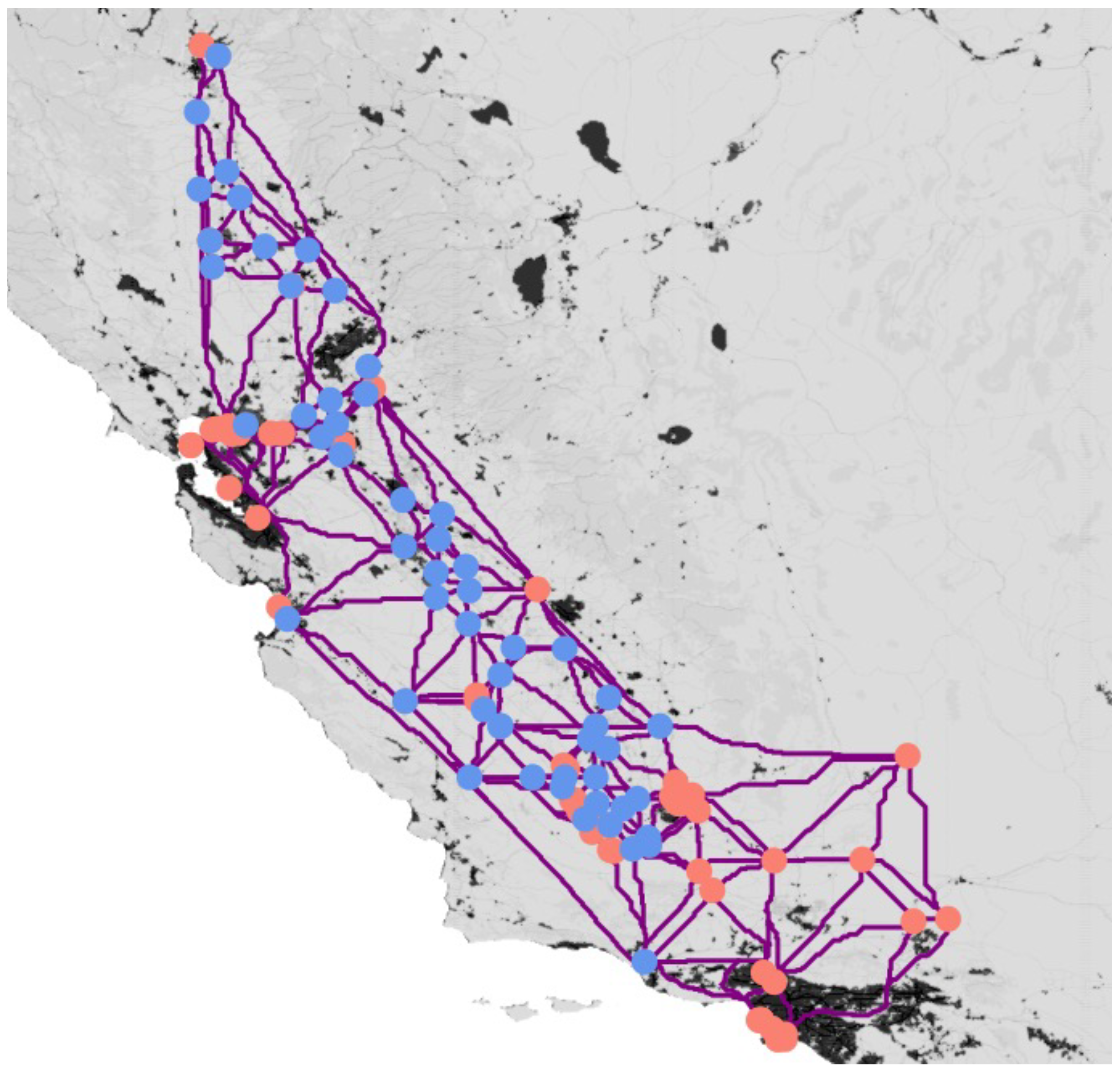
The California dataset is presented in Figure 2.

A total of 57 scenarios were generated by sampling each of the storage sites’ storage capacity probability function to obtain a random annual storage capacity value for each scenario. Each scenario is parameterized to process 17 MtCO₂/yr for 30 years. 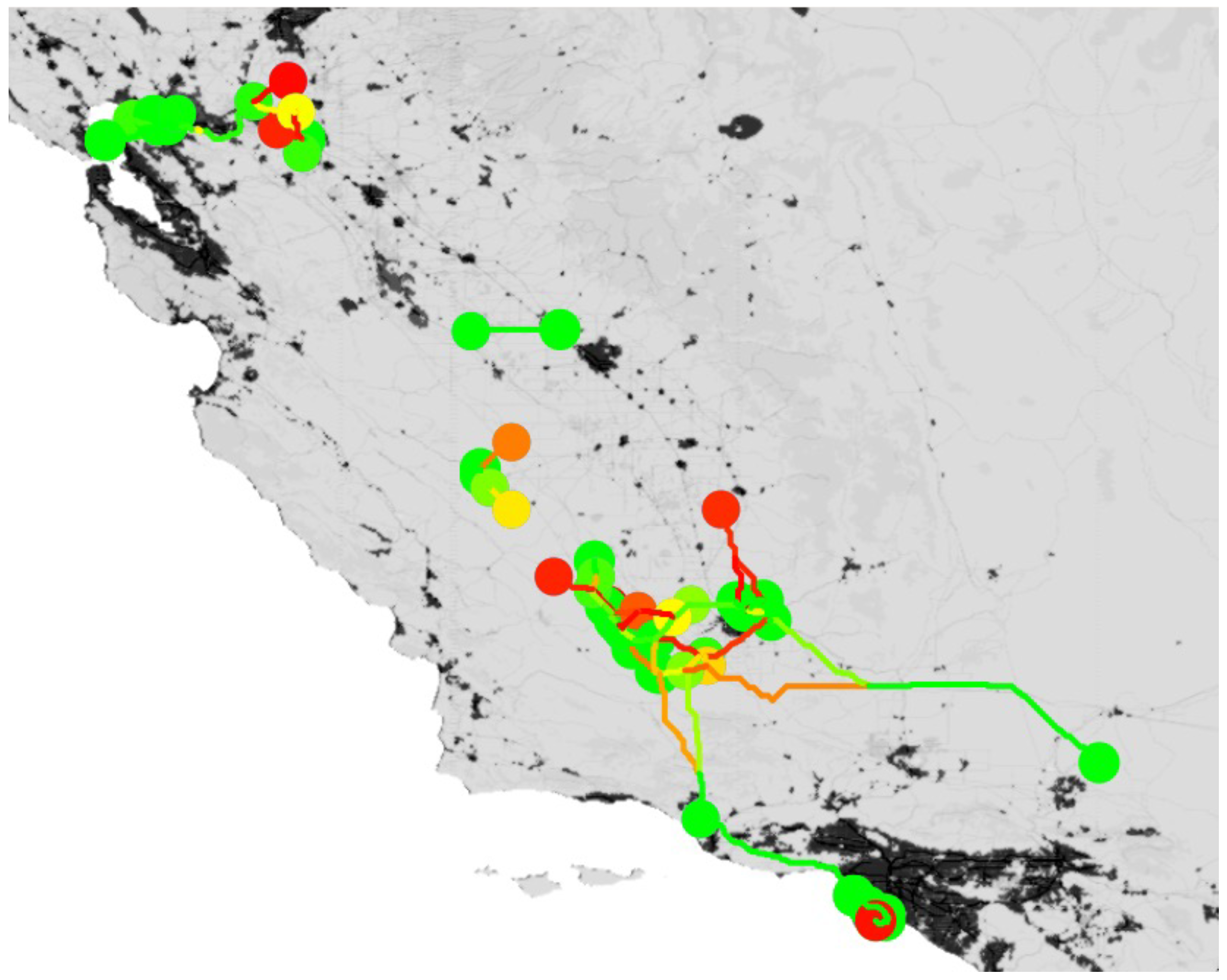Optimal solutions for each scenario were found by solving the MILP from Section 2 using $SimCCS$ and IBM’s CPLEX optimization software version 12.9 [7]. The heatmap was generated by aggregating the deployed infrastructure from the solutions of the 57 scenarios and calculating the commonality score for each infrastructure component. The commonality score was translated into a value in the range $[0,1]$, representing the percentage of scenario solutions in which the component appears, by dividing by 57. The resulting heatmap is presented graphically by mapping the commonality score into a color on the red–yellow–green color gradient, as seen in Figure 3.

The core infrastructure is constructed by first identifying the desired risk index in the range of $0\%$ to $100\%$. As described in Section 3, this threshold relates to the minimum percentage of scenarios in which each network component must appear to be available in the core infrastructure solution. The selection of a risk index filters out infrastructure from the full heatmap that is below the threshold to exclude it from possibly being in the core solution. After the infrastructure available to the core solution is identified, the capacity for each sink is set as described in Section 3 to be the X^th percentile of the corresponding probability distribution. 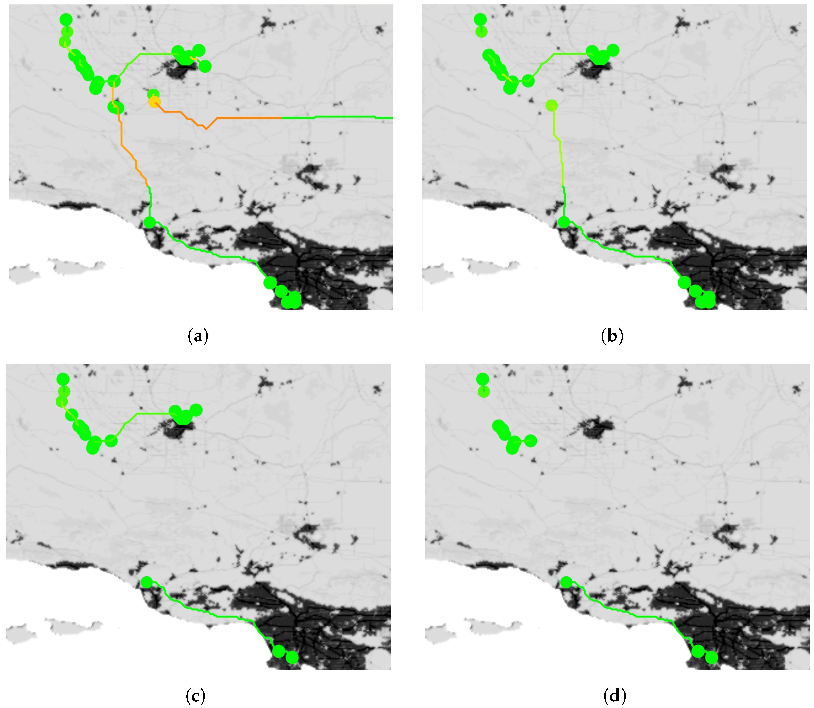Finally, the minimum-cost maximum flow is calculated using the standard process of first finding the maximum flow using the Ford–Fulkerson algorithm and then finding the minimum-cost flow with that value using integer linear programming [44]. Core infrastructure found by this process for a subregion of the dataset using risk index values of $100\%$, $43\%$, $30\%$, and $15\%$ is presented in Figure 4.

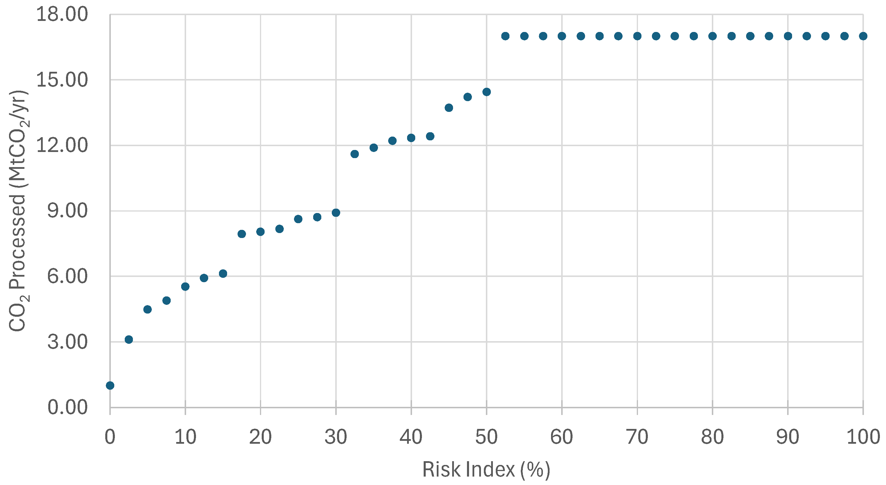
Increasing the risk index corresponds to generating more conservative infrastructure, as the amount of available infrastructure is restricted and the storage capacity is reduced. The trade-off between the risk index and performance is important for decision-makers to consider, since this can provide insight into the potential range of performance as well as the natural risk index breakpoints that should be considered. The performance measures that are of most interest are the amount of CO₂ that the identified core infrastructure is able to process and the cost of the infrastructure. To quantify this trade-off, the proposed core infrastructure generation process was run for risk index values from $0\%$ to $100\%$ in $2.5\%$ increments.

Figure 5 presents the trade-off curve between the selected risk index and the amount of CO₂ that can be processed by the identified infrastructure. Reducing the risk index from $15\%$ to $0\%$ reduced the amount of CO₂ processed by $83.7\%$. Likewise, reducing the risk index from $30\%$ to $15\%$ reduced the amount of CO₂ processed by $31.3\%$. This demonstrates the trade-off between infrastructure effectiveness and assumption of risk.

Of particular interest are the obvious breakpoints that may help decision-makers settle on a specific risk index or small set of risk indices. For example, the difference in the amount of CO₂ processed when the risk index is decreased from $17.5\%$ to $15\%$ ($1.81$ MtCO₂/yr) is notably more than the difference between $20\%$ and $17.5\%$ ($0.09$ MtCO₂/yr) or $15\%$ and $12.5\%$ ($0.21$ MtCO₂/yr). These breakpoints occur when infrastructure components are added to the available infrastructure that are important enough to notably increase the amount of CO₂ that can be processed by the solution. They serve as logical spots that demonstrate the most impactful trade-offs between performance and risk index. The annual amount of CO₂ processed is constant for risk index values below $50\%$ because, for this specific dataset, that commonality score encompasses all of the deployed infrastructure in all of the scenarios. This means that for low risk index values, the same infrastructure is available, as opposed to higher risk index values, when the required commonality score reduces the amount of available infrastructure. The non-increasing trend from a large amount of CO₂ processed for low risk index values to a small amount of CO₂ processed for high risk index values would be seen for all datasets, as the amount of available infrastructure is reduced. The constant regions, breakpoint locations, and CO₂ processed values are dataset-specific; accordingly, other datasets would likely show differences in this behavior.

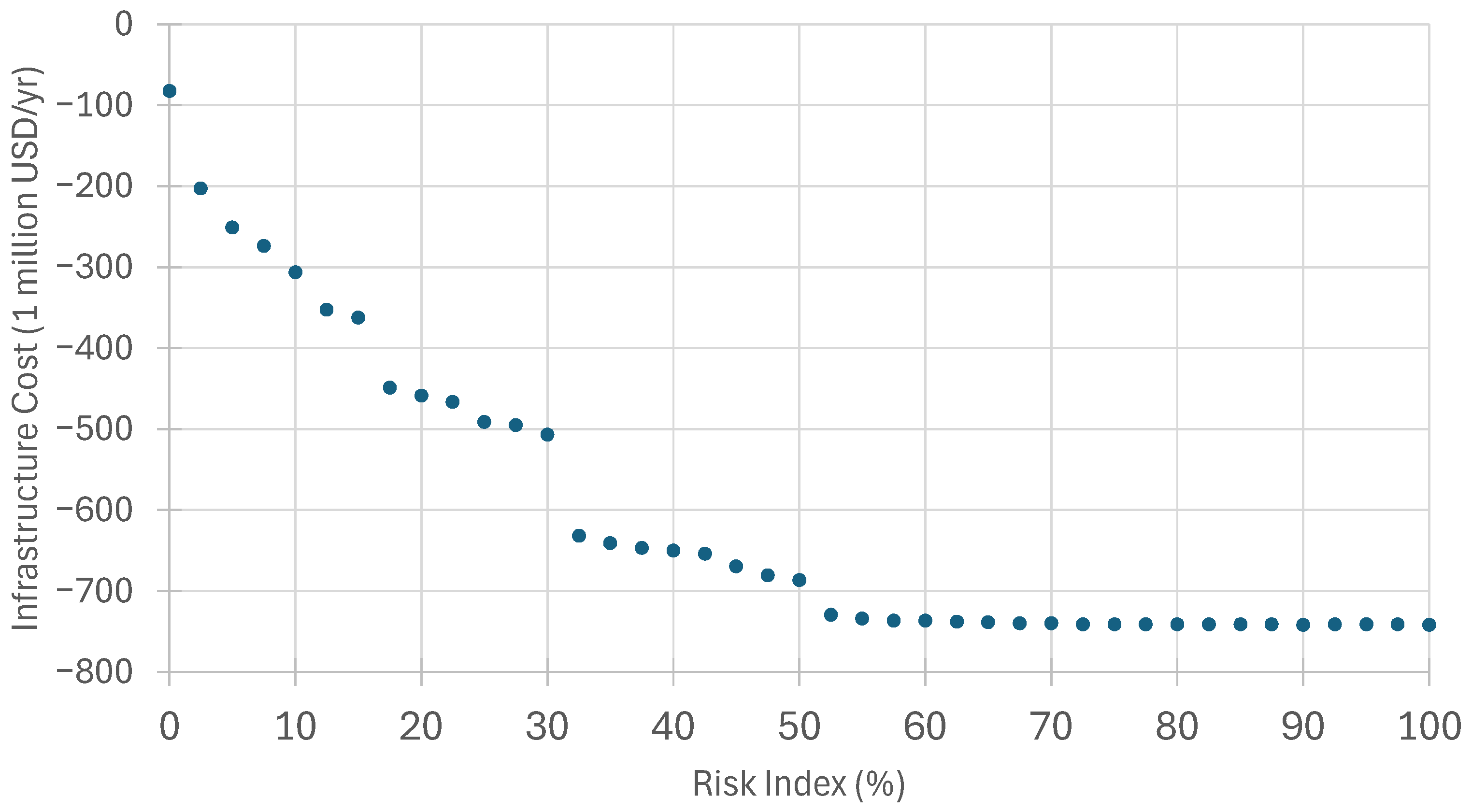
Figure 6 presents the trade-off curve between the selected risk index and the cost of the identified infrastructure. Note that the inclusion of LCFS and $45Q$ credits allows for the cost of processing CO₂ to be outweighed by the credits, which enables the infrastructure to have a negative cost (i.e., to be profitable). Reducing the risk index from $15\%$ to $0\%$ decreased the profit of the project by $77.1\%$. Likewise, reducing the risk index from $30\%$ to $15\%$ decreased the profit of the project by $28.5\%$. This demonstrates the trade-off between infrastructure cost and assumption of risk. The same breakpoints (for the same risk index values) are seen in the cost trade-off curve as in the trade-off curve for the amount of CO₂ processed.

5. Conclusions

This paper introduces a novel workflow for designing cost-effective CCS infrastructure that is robust to storage site performance uncertainty. Employing a Monte Carlo-inspired approach, the proposed process samples storage capacity distributions to generate multiple infrastructure scenarios, solves each scenario optimally using an MILP model, and aggregates the results into a heatmap. By allowing decision-makers to specify a risk tolerance through a risk index parameter, the workflow identifies core infrastructure components that balance performance with resistance to requiring repair during actual injection operations due to storage uncertainty.

The evaluation of this workflow using the California dataset from the DOE’s CUSP project demonstrated its effectiveness in generating actionable insights for large-scale CCS deployments. The results highlighted the significant trade-offs between risk index, CO₂ processing capacity, and cost, offering stakeholders a structured framework to select infrastructure configurations that align with specific operational and financial priorities. Specifically, reducing the risk index from $15\%$ to $0\%$ led to an $83.7\%$ reduction in CO₂ processing capacity and a $77.1\%$ decrease in project profit, illustrating the cost of adopting a more conservative infrastructure strategy. Notably, the workflow identifies critical breakpoints where small adjustments in the risk index lead to disproportionate shifts in infrastructure performance, allowing decision-makers to pinpoint cost-effective trade-offs between risk and cost/performance. By quantifying these relationships, the approach provides a flexible method for optimizing CCS network design under storage uncertainty.

Future work could expand on this effort by incorporating additional sources of uncertainty, such as the possibility of pipeline failure, capture or storage cost variability, or regulatory uncertainty. Different risk index values for each individual storage site could be explored as well. This could be done by setting the risk indices on an individual site-by-site basis instead of having the same risk index for all sites. This would allow the risk index for individual storage sites to be adjusted to account for a insights into real-world data quality or experimental desires. Enhanced geological models could further refine the storage capacity distributions, increasing the realism and applicability of the methodology. Finally, it is likely that the breakpoints observed in testing on the California dataset will exist at different risk index values for other datasets. Testing the workflow on other regions with different storage performance profiles and larger numbers of sources, sinks, and possible pipeline networks would help generalize its utility and validate its scalability.

This workflow represents a significant step toward addressing the challenges of planning CCS infrastructure under uncertainty, offering a flexible and robust tool for stakeholders aiming to deploy large-scale CCS networks with confidence in their performance and economic viability.