2. The Proposed Method
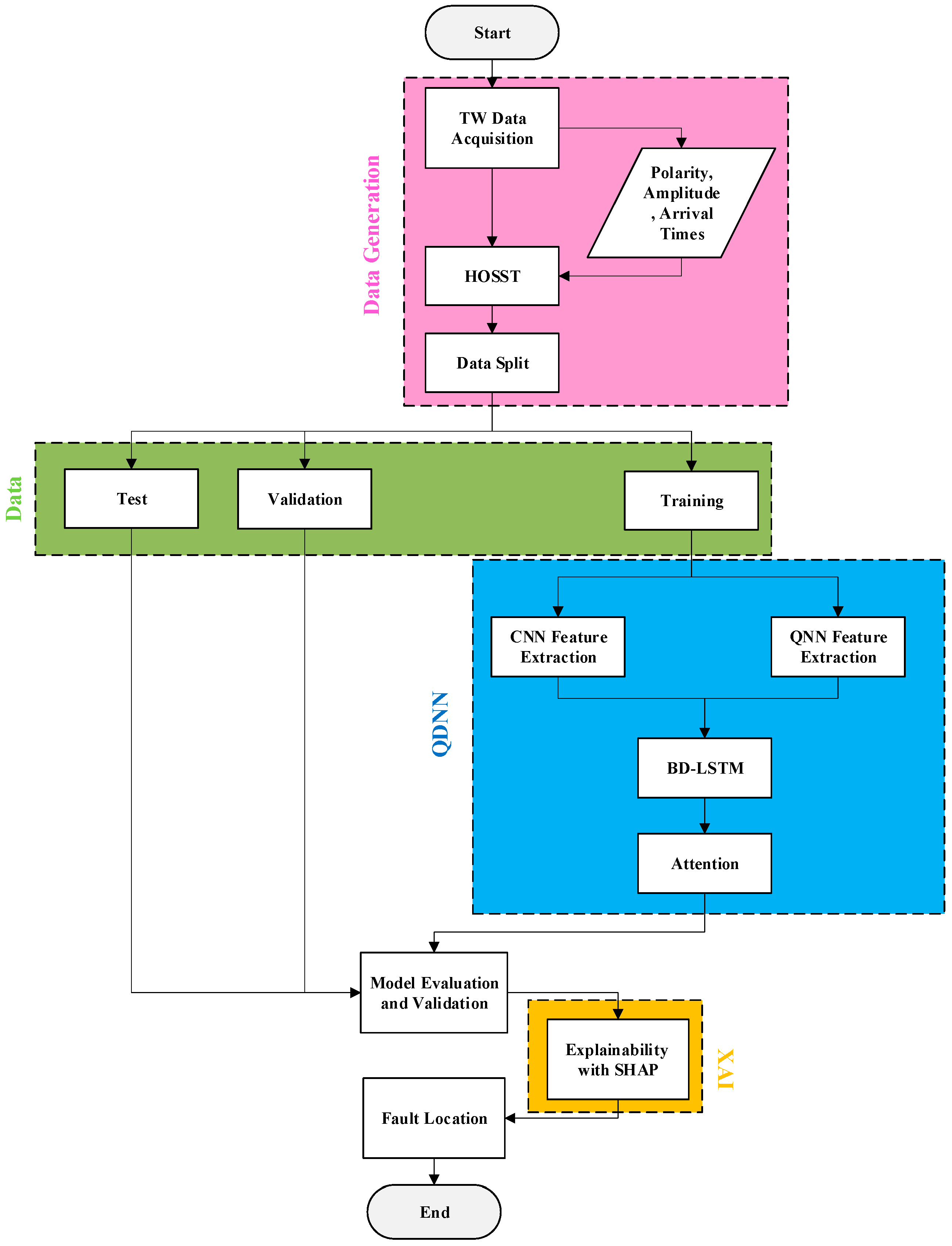
The proposed method combines HOSST for feature extraction with a QDNN to detect and locate faults in DCMGs. HOSST captures key fault characteristics, while the QDNN integrates classical and quantum neural networks for enhanced data processing. Temporal patterns are identified using a BD-LSTM and attention mechanism, and XAI ensures transparent and reliable results. The method is adaptable to various DCMG setups.
2.1. Feature Extraction Based on HOSST
Effective feature extraction from current signals plays a pivotal role in detecting faults accurately in DCMGs, especially for TW-based protection. This is achieved through a HOSST, a higher order of the initial version of synchrosqueezing transform (SST), which offers a more concentrated and accurate time–frequency representation, crucial for detecting fault-induced TWs due to capturing high-frequency contents from input signals.
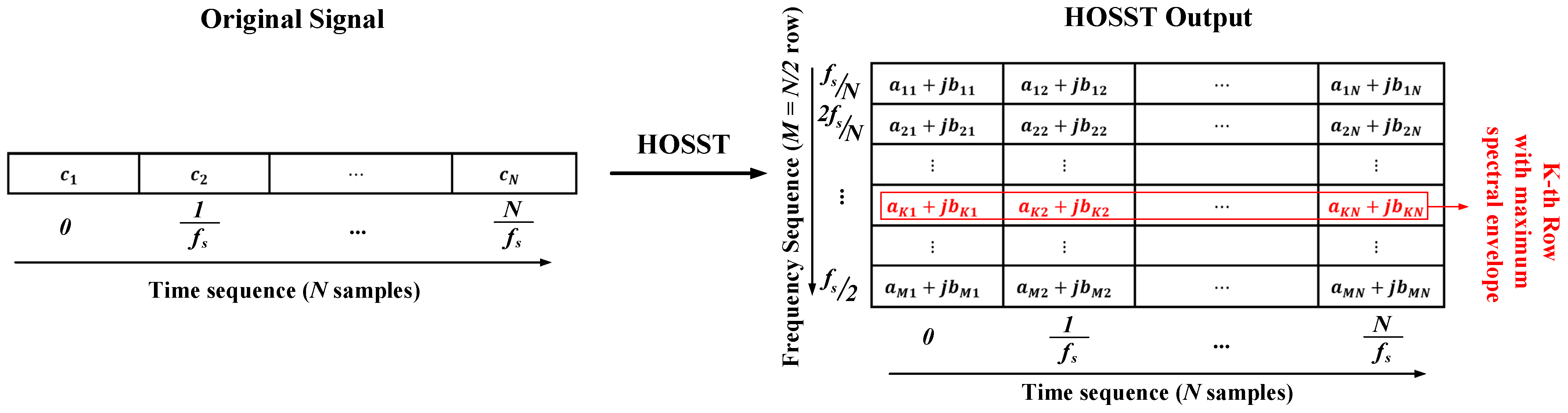
Figure 1 provides a schematic representation of the HOSST process. On the left, the original time-domain signal is shown as a sequence of sampled data points, where each sample corresponds to a specific time step. HOSST then transforms this time-domain signal into a time–frequency representation, illustrated on the right. In the output, each row corresponds to a specific frequency bin, and each column represents a time step. The red-highlighted row indicates the frequency bin with the maximum spectral energy for a given time sample, which is crucial for detecting and analyzing transient events like TWs. This visualization simplifies the interpretation of HOSST results, allowing operators to identify the most relevant frequency components for fault detection in DCMGs. In fact, by concentrating spectral energy into distinct frequency bins, HOSST ensures the preservation of transient fault characteristics, which are often diluted in traditional frequency-domain analysis. This enhanced clarity in feature extraction not only improves the accuracy of fault detection but also simplifies the interpretability of fault dynamics for system operators.
HOSST enhances classical synchrosqueezing by reallocating frequency components using higher-order Taylor series expansions, designed to refine time–frequency location for transient events such as TWs, defined as Equation (1).
where
denotes the angular frequency, defined as
, where
is the frequency of the signal component. This term plays a crucial role in the time–frequency representation by determining the spectral resolution in the synchrosqueezing process;
represents the high-order synchrosqueezed time-frequency representation,
denotes the normalization factor of the wavelet,
is the short-time Fourier-based synchrosqueezing transform,
depicts the frequency components derived using high-order derivatives,
is the Dirac delta function to reallocate the time–frequency energy for higher concentration, and
is a threshold parameter used to reduce noise effects by filtering out low-energy components. Finally, the chosen order to capture TWs is considered the third order.
Equation (1) represents the high-order synchrosqueezed time-frequency representation, which refines the localization of transient events such as TWs. By redistributing frequency components using higher-order derivatives, it enhances fault detection accuracy.
2.2. Obtaining the Magnitude and Polarity of TWs
The magnitude of TWs is calculated as the modulus of the complex output from HOSST at the frequency corresponding to the maximum value of the spectral envelope, given by Equation (2).
Here, is the frequency at which the spectral envelope has its maximum value, and is the FSSTH output for the selected order .
The polarity of TWs is determined by the phase angle of the complex HOSST output at
. The formula is shown in Equation (3):
This provides the direction of propagation, which is essential for fault localization. Equation (3) calculates the polarity of TWs by determining the phase angle of the complex HOSST output at the dominant frequency. This helps distinguish between wave directions, which is crucial for accurate fault localization in DCMGs.
2.3. Data Preparation
After determining the magnitude and polarity of TWs, the TOA, magnitude, and polarity of the first and second TWs are recorded. These parameters are measured relative to the reference bus, which is the point of connection between the DCMG and the main power grid. Measurements are taken incrementally along the lines, typically meter by meter, to capture accurate fault characteristics. The locations of TWs are recorded cumulatively, meaning the distances are calculated from the reference bus to the farthest fault point. The maximum distance from the reference bus is used as the output vector, representing the fault location in relation to the microgrid connection point. This process ensures precise input data preparation for fault localization and enhances the accuracy of the proposed method.
The data is first shuffled randomly to ensure unbiased distribution. The structured data preparation process ensures that the model is trained on a representative dataset, minimizing bias and enhancing generalizability. This approach not only improves the reliability of the fault localization predictions but also facilitates smoother integration of the model into practical fault management workflows. Therefore, 70% of the data is allocated for training, 10% for validation, and the remaining 20% for testing. These datasets are then fed into the proposed network for training and evaluation.
2.4. Proposed QDNN Architecture
Different layers of the proposed QDNN framework are listed as follows:
The output consists of expectation values derived from the quantum measurements, which represent the quantum-enhanced features.
Merging paths, in which the outputs of the CNN and QNN are concatenated to combine the local features extracted by the CNN with the quantum-based features from the QNN.
BD-LSTM layer, to which the merged features are passed. It processes sequential dependencies in the data, learning patterns over time from both directions.
The attention layer, which focuses on the most important temporal features from the BD-LSTM output, assigns higher weights to these features to enhance the model’s understanding of key data points, and reduces noise and improves the interpretability of predictions. This design choice aligns with the need for fault localization systems to prioritize critical data points while discarding less relevant information.
Fully connected layer, into which the output from the attention layer is fed. It is a dense layer with 128 neurons, and ReLU activation further processes the combined features.
The output layer, the final layer, is a dense layer with a single neuron that produces the model’s prediction, which could represent a fault location.
The architecture of the proposed network is depicted in
Figure 2.
2.5. XAI Integration
In the final stage of the proposed method, an XAI approach is integrated to enhance the interpretability of the model’s predictions for fault location in DCMGs. The goal is to explain how the model makes decisions and highlight the key factors affecting fault detection.
The XAI technique utilized in this study is SHAP, which quantitatively helps explain which factors most influence the model’s predictions. SHAP explains how factors such as the time of arrival, magnitude, and polarity of the TWs contribute to the fault location estimation. The SHAP value, i.e.,
, for a feature
is calculated as Equation (4).
Here is a subset of features excluding represents the full set of input features, is the model’s prediction based on the features in , and denotes the model’s prediction when is added to . Equation (4) represents the SHAP value calculation, which quantifies the contribution of each input feature to the model’s predictions. This allows operators to understand which factors most influence fault location estimation, improving model transparency and interpretability.
After the QDNN predicts the fault location for various scenarios, SHAP decomposes the predictions into contributions from each input feature. For instance, if the predicted fault location deviates significantly, SHAP can reveal whether the variation is due to delays in TW TOAs, changes in magnitude, or polarity shifts. This integration of XAI into the proposed method bridges the gap between model predictions and practical fault analysis in DCMGs. By providing detailed insights into the model’s predictions, XAI empowers system operators to prioritize critical fault parameters, enhancing the reliability and safety of microgrid operations.
The flowchart of the proposed method is shown in
Figure 3.
2.6. Evaluation Metrics
To evaluate the performance of the proposed method in fault location estimation, six metrics are employed: root mean squared error (RMSE), mean absolute error (MAE), R-squared (R
2), Theil’s U statistic (TUS), Willmott’s index of agreement (WIA), and variance accounted for (VAF). These metrics provide a comprehensive assessment of the model’s accuracy and reliability, as defined in Equations (5)–(10), respectively. Each metric highlights a specific aspect of model performance, offering a comprehensive evaluation [
29].
Smaller values of RMSE, MAE, and TUS indicate higher accuracy, while R2, WIA, and VAF values closer to 1 reflect better performance. Specifically, the definition of each one is listed as follows:
RMSE measures the average magnitude of error between the predicted and actual values. It penalizes larger errors more heavily, making it a reliable indicator of overall accuracy.
MAE calculates the average absolute difference between predicted and actual values, offering an easily interpretable measure of error without penalizing outliers as strongly as RMSE.
R2 evaluates the proportion of variance in the actual values that is explained by the predictions. Values closer to 1 indicate a better fit.
TUS measures the relative accuracy of predictions compared to a naïve forecasting model. Lower values indicate better performance.
WIA reflects how well the model captures the variation in the data. It considers both the error magnitude and the distribution of errors, with values closer to 1 indicating higher agreement between predictions and actual values.
VAF quantifies the percentage of variance in the actual data that is explained by the predictions. A higher VAF indicates better performance.
where
is the number of samples,
represents the actual value,
denotes the predicted value,
is the mean of actual values, and
is the variance. The use of diverse evaluation metrics ensures that the model’s performance is assessed from multiple perspectives, capturing both the accuracy of predictions and the robustness under varying operational conditions. This holistic evaluation framework aligns with the industry’s need for reliable and interpretable fault localization methods.
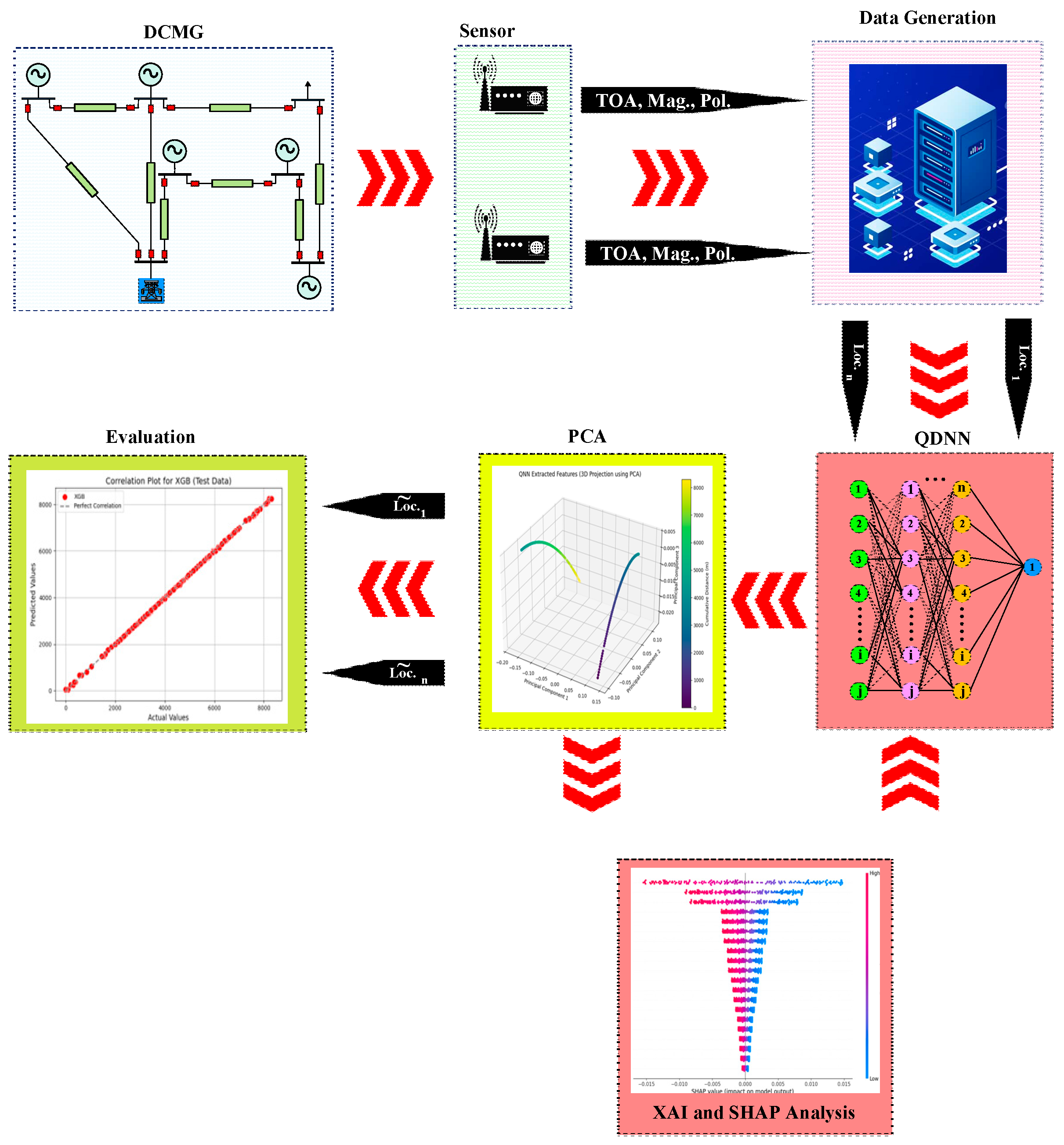
The overall workflow of the proposed fault detection and localization methodology is illustrated in
Figure 4.
3. Results
To demonstrate the effectiveness of the proposed methodology, it was applied to a medium-voltage DCMG, with detailed specifications provided in
Table 2 and a schematic representation shown in
Figure 5. To evaluate the model’s performance, DC faults were simulated at intervals of 50 m throughout the system. These faults included positive pole-to-ground, negative pole-to-ground, and pole-to-pole scenarios, covering the entire system up to its endpoint.
The generated data were divided into three sets for model evaluation: 70% (896 samples) was allocated for training, 10% (128 samples) for validation, and the remaining 20% (257 samples) was used for testing, in which TOA of first and second TW, the magnitude and the polarity of them, are regarded as the input vector to the learning model. This comprehensive dataset ensures a robust assessment of the proposed method across various fault types and locations.
3.1. Impact of Quantum Feature Extraction on Model Performance
To evaluate the effectiveness of the proposed method, the model was trained using the prepared dataset. The primary objective was to assess the impact of quantum-based feature extraction on fault location accuracy. The integration of quantum feature extraction not only reduces error rates but also highlights the interactions between key features, as evident in the model’s consistent performance across all datasets. This deeper understanding of feature dynamics offers a unique advantage in designing future systems with improved reliability. For this purpose, the system was run under two configurations:
The first configuration involved training and testing the system without the quantum feature extraction path. Only the CNN was used to extract features.
In the second configuration, the QNN was added alongside the CNN for feature extraction, leveraging quantum-enhanced capabilities.
Table 3 provides a comparison of prediction performance metrics between the proposed QDNN and a standard DNN without quantum enhancements. The table includes six evaluation metrics. The results highlight that the RMSE and MAE values for QDNN are consistently lower than those of the standard DNN across all datasets, indicating reduced prediction errors. The R
2, WIA, and VAF values for QDNN are closer to 1, demonstrating the superior accuracy and reliability of the proposed method. Finally, the TUS values for QDNN are smaller, confirming better fault location estimation accuracy.
These results confirm that incorporating quantum feature extraction significantly enhances the model’s performance, especially in reducing error rates and improving prediction accuracy across diverse datasets.
3.2. Principal Component Analysis (PCA) and Feature Extraction Performance of QNN for Fault Localization
The analysis of the QNN-extracted features provides a detailed understanding of its effectiveness in fault location for DCMGs.
Table 4 displays the loadings of each input vector component on the first three principal components (PCs) obtained through the PCA projection of QNN-extracted features. These loadings quantify the contributions of input features such as the TOA, magnitude, and polarity of the TWs to each PC. Each loading reflects the contribution of the corresponding feature to the variance captured by the PCs. Higher loadings indicate the greater influence of the feature on the respective PC. For instance, the polarity of the second TW shows the highest loading on PC1, signifying its dominant role in fault localization accuracy.
The results in
Table 4 show that specific features, such as the polarity of the second TW and the TOA of the second TW, contribute significantly to PC1 and PC2, respectively. These features capture key aspects of the fault dynamics, enhancing the interpretability of the extracted feature space. The polarity of the first TW also plays a crucial role in refining fault localization through PC3. For PC1, which captures the highest variance (92.86%), the polarity of the second traveling wave exhibits the most significant contribution with a loading of 0.78996, followed by the magnitude of the second TW with a loading of −0.46681. These features play a dominant role in fault location, emphasizing their importance in the QNN’s feature extraction process. PC2, which explains an additional 7.03% of the variance, is heavily influenced by the TOA of the second TW, showing a loading of 0.902457. This highlights the significance of temporal features in capturing the behavior of faults. PC3, accounting for 0.11% of the variance, primarily incorporates the magnitude of the second TW (0.614752) and the polarity of the first TW (0.542118), refining the fault localization accuracy.
Table 5 summarizes the explained variance ratio and cumulative variance for the first three PCs. The cumulative variance reaches 99.99%, demonstrating that almost all critical information from the QNN-extracted features is retained within these three components. This indicates the effectiveness of PCA in reducing the dimensionality of the feature space while preserving the most essential fault-related characteristics.
The results in
Table 5 highlight the effectiveness of PCA in dimensionality reduction. The first PC captures 92.86% of the variance, and the first three PCs together retain 99.99% of the variance. This demonstrates that PCA preserves nearly all critical information from the original data while reducing the feature space, ensuring efficient input to the QDNN model. Moreover,
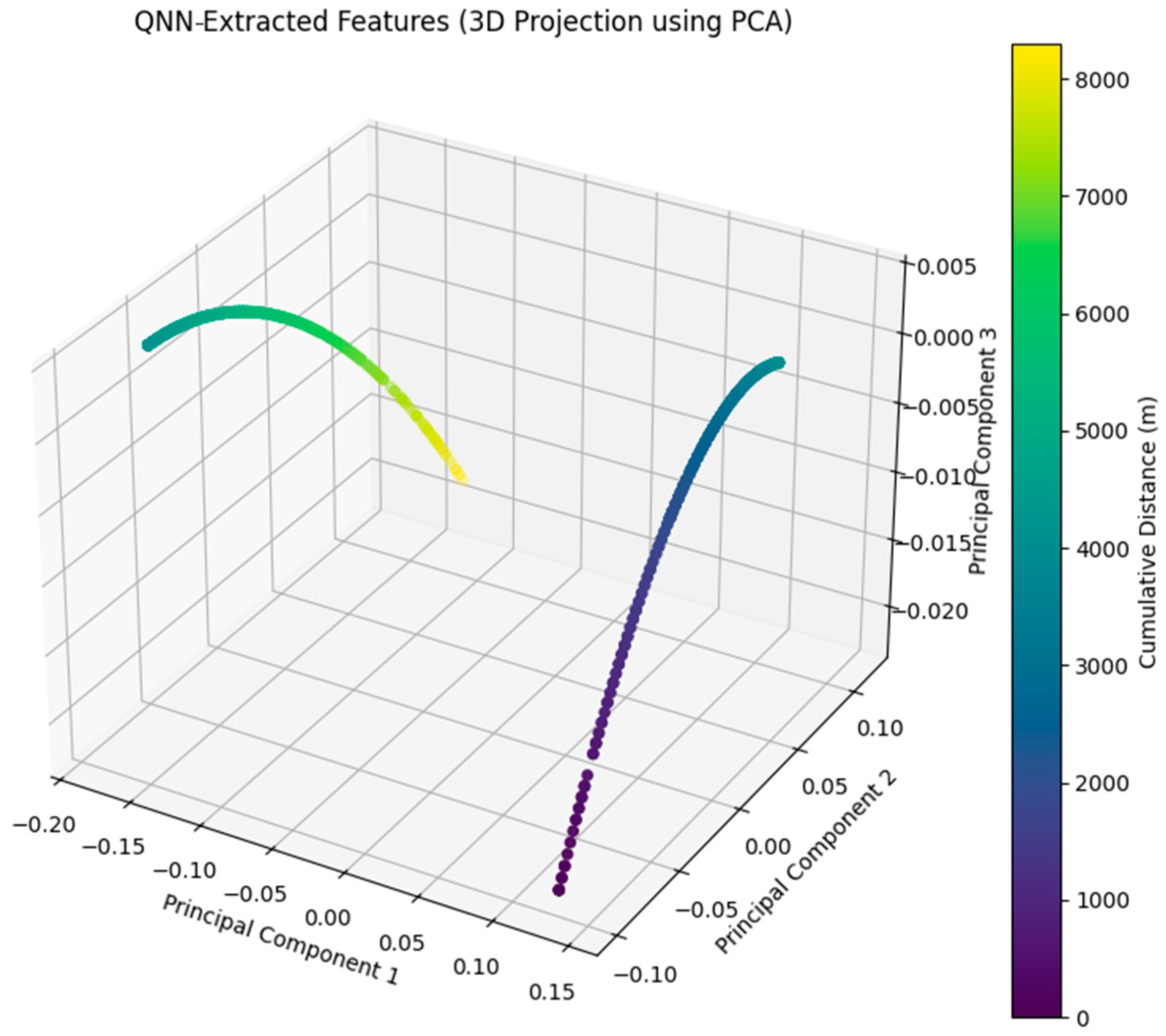
Figure 6 provides a visualization of the QNN-extracted features in a 3D space after PCA projection.
The points are color-coded based on the cumulative distance of faults (in meters), illustrating distinct clusters corresponding to different fault scenarios. This clustering demonstrates that the QNN successfully transforms raw input features into a structured feature space, enabling clear differentiation between fault locations. The smooth distribution of data points further validates the robustness of the proposed method in handling variations in fault characteristics.
Finally, the reconstruction error is calculated as 0.000525039, which highlights the negligible loss of information during the PCA transformation. This low error validates the reliability of combining QNN with PCA for feature extraction and dimensionality reduction. The ability to preserve critical information ensures that the reduced feature space is highly representative of the original input data.
3.3. XAI Analysis of DNN and QDNN Models
The integration of XAI methods into the proposed framework provides a deeper understanding of the decision-making process for both the standard DNN and the QDNN. The analysis focuses on comparing the feature importance and interpretability of these two models using SHAP. The SHAP analysis further enables a granular understanding of how each feature impacts the fault localization process. By breaking down complex interactions into intuitive visualizations, the proposed framework bridges the gap between advanced machine learning techniques and practical fault management strategies, empowering engineers to make informed decisions. The results are presented in
Figure 7 and
Figure 8, where the impact of input features on the fault location predictions is visualized and quantified.
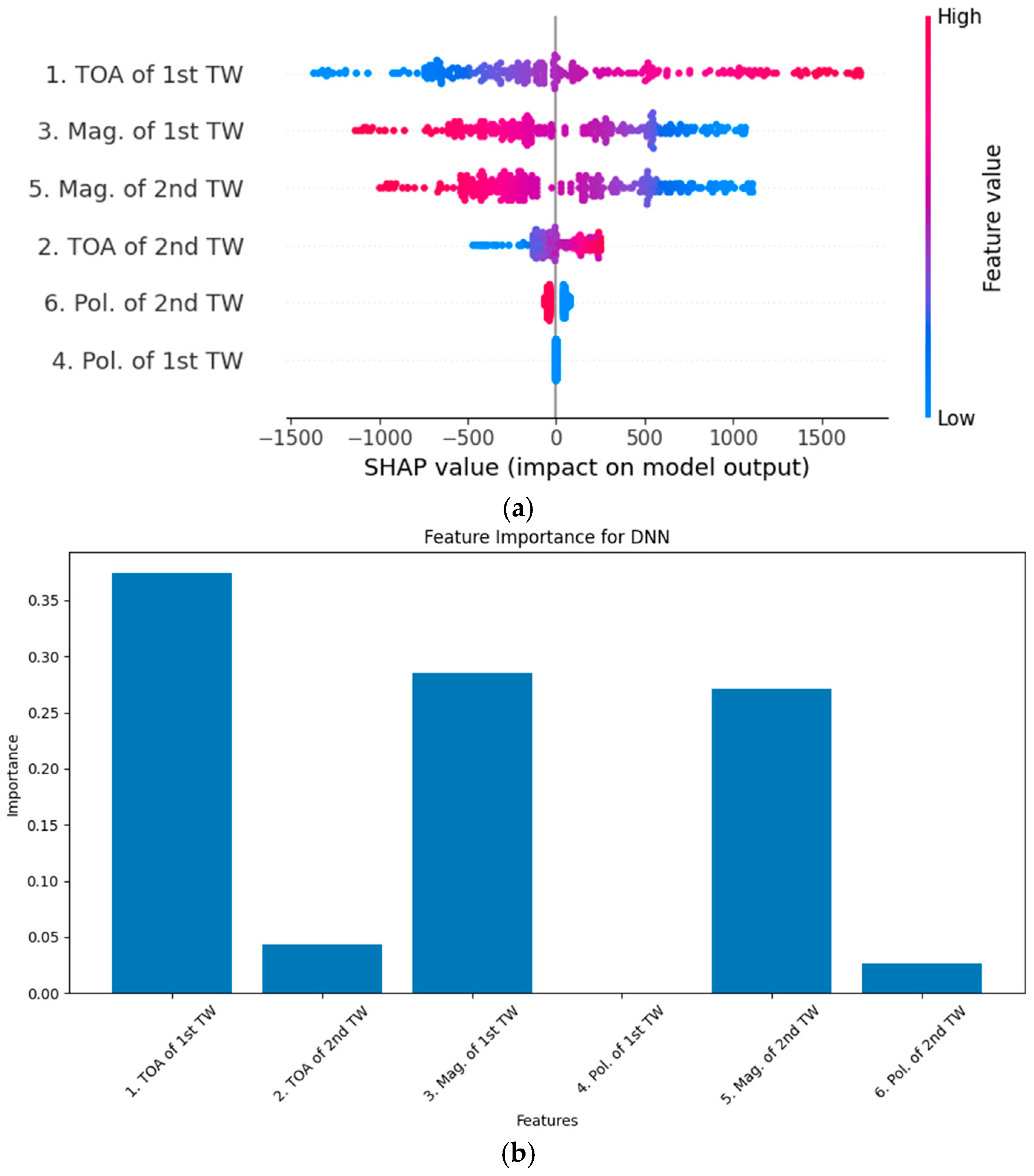
Figure 7a shows the SHAP summary plot for the DNN-based fault location model. The plot highlights the impact of each input feature on the model’s output. As can be seen, the TOA of the first TW has the highest impact on the model’s predictions, with a wide range of SHAP values reflecting its critical role in fault localization.
Furthermore, the magnitude of the first TW and the magnitude of the second TW also contribute significantly, indicating their importance in capturing fault characteristics, while the polarity of both the first and the second TWs has a relatively smaller impact, suggesting these features play a secondary role in the DNN’s decision-making process.
Figure 7b provides a bar chart of feature importance derived from the SHAP values. The results confirm that temporal and magnitude-based features dominate the fault location predictions, with the TOA of the first TW and the magnitude of the first TW being the most influential. Similarly,
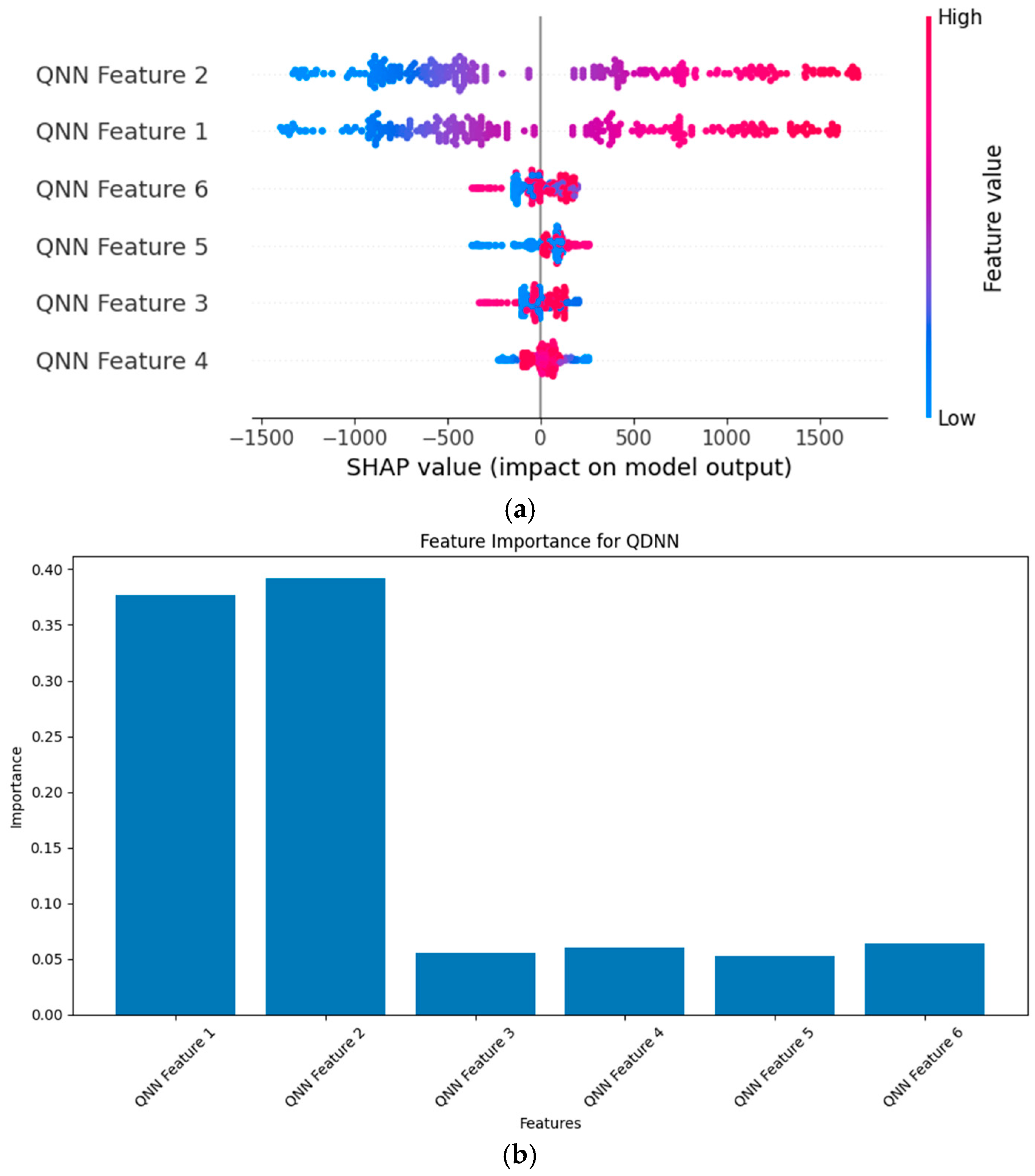
Figure 8a illustrates the SHAP summary plot for the QDNN-based fault location model, where the input features are quantum-enhanced.
As can be seen, QNN Feature 2 exhibits the highest impact on the model’s output, as indicated by its large range of SHAP values. This feature encapsulates quantum-enhanced information related to fault scenarios, which significantly improves interpretability and accuracy. Other QNN-derived features (QNN Features 1, 3, 4, 5, and 6) contribute to the model’s predictions but with relatively smaller impacts compared to QNN Feature 2. The SHAP values for QDNN show more concentrated patterns compared to the DNN, reflecting the QDNN’s enhanced ability to process fault-related information effectively.
Figure 8b presents the feature importance bar chart for the QDNN. It confirms that QNN Feature 2 dominates the fault location predictions, with a significantly higher importance score compared to other features, which highlights the advantage of integrating quantum feature extraction in the proposed framework.
Based on
Figure 7 and
Figure 8, the comparison between DNN and QDNN demonstrates the superiority of the QDNN model in capturing and utilizing critical fault information, which can be summarized as follows:
The DNN relies heavily on temporal features like the TOA of the first TW, which, while effective, lack the advanced representation provided by quantum-enhanced features.
The QDNN, by contrast, leverages quantum-derived features that encapsulate complex relationships within the fault data, leading to more precise and interpretable predictions.
The SHAP analysis highlights that the QDNN’s predictions are more robust, with fewer outliers in SHAP values and a clear dominance of specific quantum features.
4. Discussion
In this section, the proposed QDNN is compared with five baseline models: extreme gradient boost (XGB) regressor, k-nearest neighbors regressor (KNN), recurrent neural network (RNN), support vector regressor (SVR), and multilayer perceptron regressor (MLP). The goal of this comparison is to evaluate the performance of these methods in fault location prediction and to demonstrate the superiority of the proposed QDNN framework.
First, to better understand the aforementioned models, these methods are explained:
The XGB is a gradient-boosting framework that builds decision trees sequentially, where each tree attempts to correct the errors of the previous ones. This method is known for its speed and efficiency, which makes it suitable for structured data. In this study, XGB was initialized with a random state of 42 to ensure consistent results during training and testing. The default parameters, such as the learning rate and tree depth, were used for simplicity and stability.
The KNN works by predicting an output value based on the average of the closest points in the feature space. The model relies on the Euclidean distance for determining similarity, and was used as the default neighbor count. Normalization of features was performed with minimum and maximum scalers to ensure fair distance calculations across features with different scales.
The RNN captures sequential patterns and temporal dependencies in data. It was implemented with a single hidden recurrent layer containing 50 units and ReLU activation for non-linearity. The data were reshaped into a 3D format to account for their sequential nature. Adam optimizer was used for training over 50 epochs, with a batch size of 32, ensuring convergence while maintaining computational efficiency.
The SVR maps input features into a higher-dimensional space using a kernel function, allowing it to capture non-linear relationships. The radial basis function kernel was employed to handle the complex patterns inherent in fault data. Parameters such as for regularization and to set the margin of tolerance were selected to balance prediction accuracy and model complexity.
The MLP is a neural network with multiple layers that maps input features to outputs through backpropagation. In this study, it was configured with two hidden layers containing 50 and 25 units, respectively. The ReLU activation function was applied for non-linearity, and the Adam solver was used for training. The training process was capped at 1000 iterations to ensure convergence and reduce computational load.
The performance metrics of these models on the training, validation, and test datasets are presented in
Table 6,
Table 7, and
Table 8, respectively. These metrics collectively provide a comprehensive evaluation of prediction accuracy and robustness.
On the training dataset in
Table 6, QDNN exhibits the best performance, with the lowest RMSE (2.051224) and MAE (0.629743), as well as near-perfect scores for R
2, WIA, and VAF. This indicates that QDNN can capture the underlying fault patterns effectively during training. In contrast, MLP shows the highest error values, suggesting overfitting or difficulty in modeling the data.
For the validation dataset according to
Table 7, QDNN maintains its superiority, achieving an RMSE of 5.130047 and MAE of 1.660156, confirming its ability to generalize to unseen data. XGB and KNN also perform reasonably well, though their error rates are higher compared to QDNN. SVR and MLP exhibit significant error rates, highlighting their limitations in handling complex fault characteristics.
Finally, on the test dataset in
Table 8, QDNN continues to outperform other methods, with an RMSE of 4.725696 and MAE of 1.490272. This demonstrates its robustness and adaptability to new fault scenarios. While XGB and KNN provide acceptable results, they fall short of the precision offered by QDNN. MLP consistently shows the poorest performance across all datasets, indicating that it struggles to model the non-linear and complex relationships inherent in fault location data.
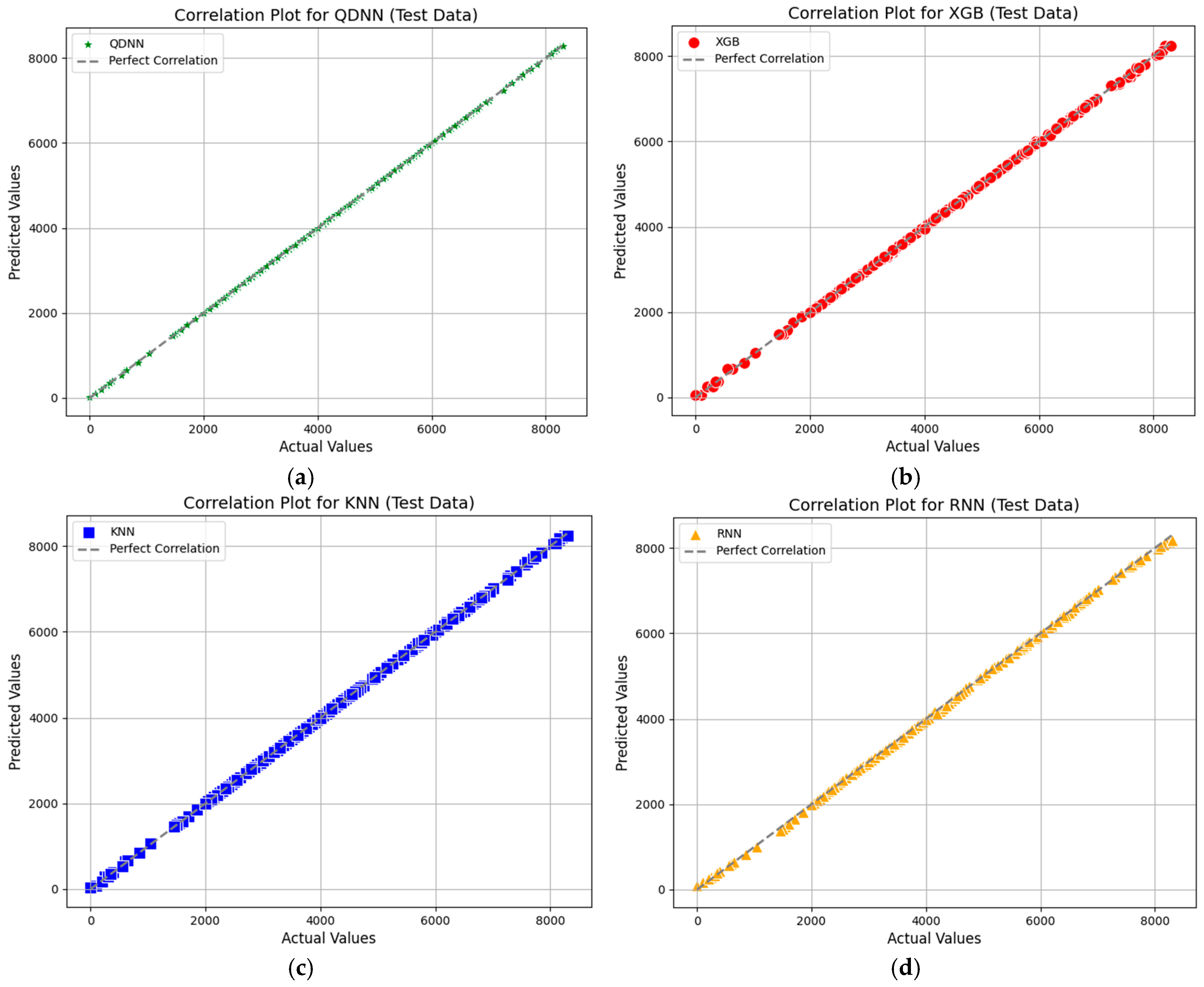
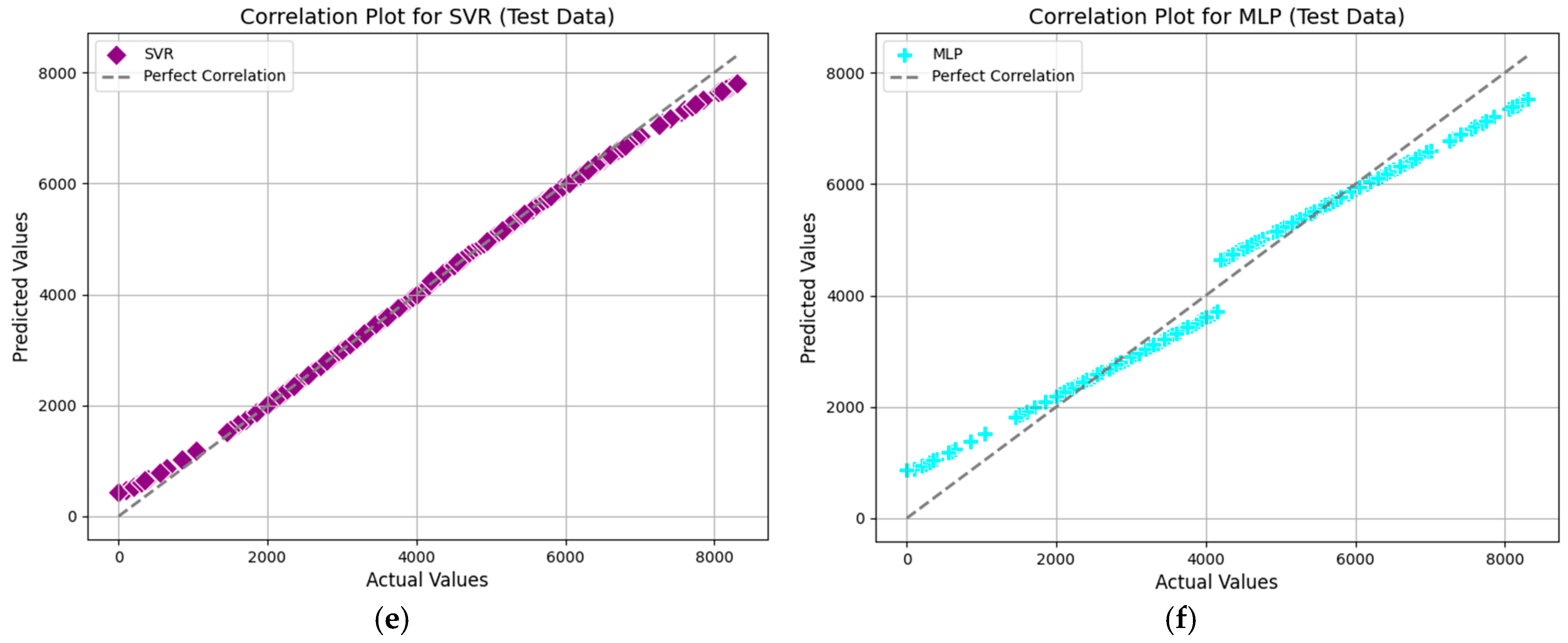
4.1. Analysis of Correlation Plots for Model Comparison
Figure 9 presents the correlation plots comparing predicted versus actual values for the test dataset across six machine learning models
. These plots are crucial for evaluating the alignment of predicted and actual values, with the diagonal line representing perfect correlation.
As can be seen in this figure, the QDNN plot demonstrates exceptional alignment with minimal errors, showcasing its ability to capture non-linear relationships effectively. XGB follows closely, with slightly larger deviations at extreme values, but remains highly reliable for complex patterns. KNN exhibits a noticeable spread, reflecting moderate prediction variability. The RNN plot highlights strong sequential modeling capabilities, though small deviations occur. SVR performs well but shows minor sensitivity to hyperparameters, visible in its scatter. MLP achieves good accuracy, with slight dispersion at higher values indicating occasional prediction inconsistencies.
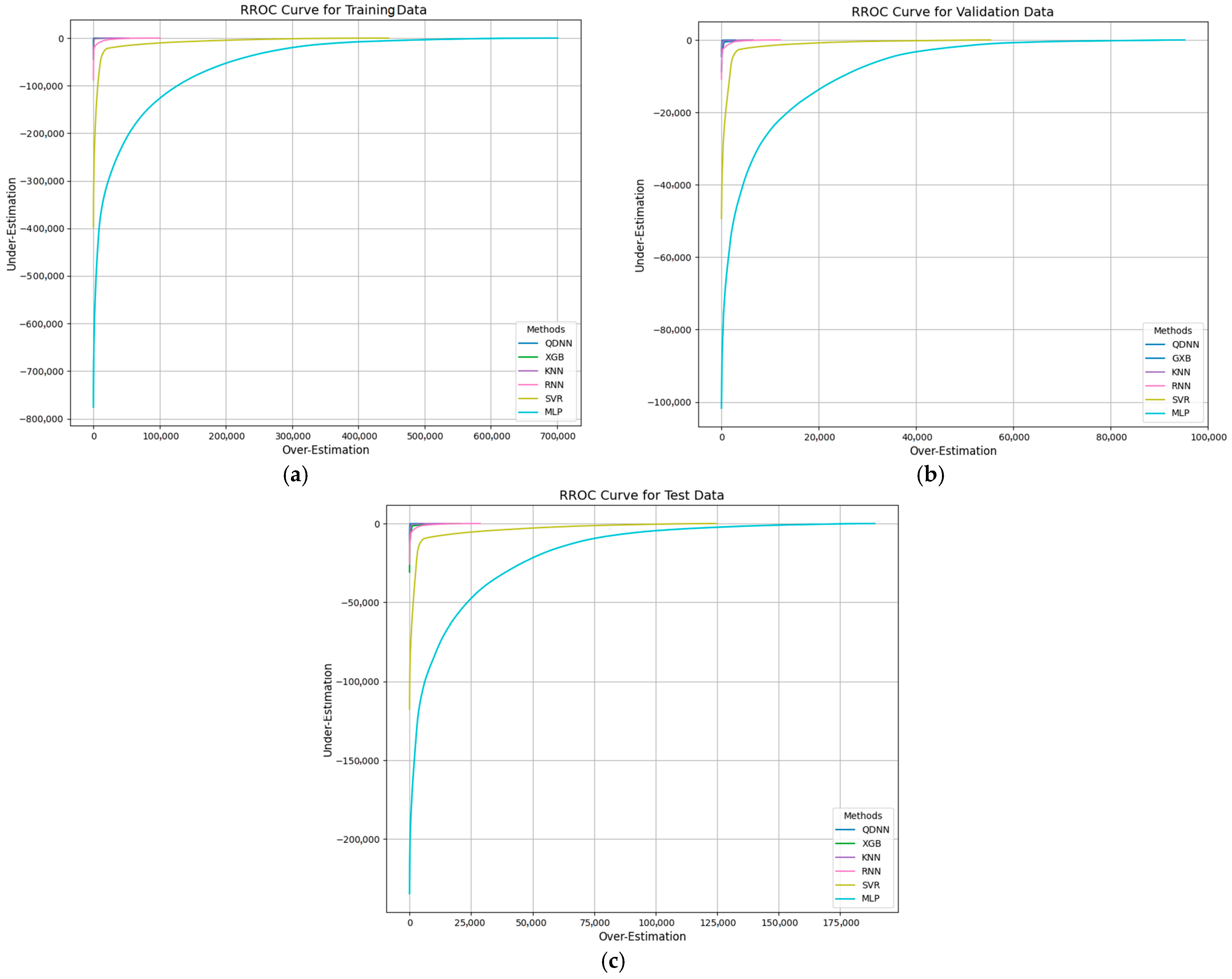
4.2. Analysis of Receiver Operating Characteristic for Regression (RROC) and Area over the Curve (AOC) Results
RROC is a visualization tool used to assess the performance of regression models by analyzing the trade-off between over-estimation and under-estimation, which considers prediction errors, plotting over-estimation on the
x-axis and under-estimation on the
y-axis. This method helps evaluate model robustness across different datasets. The AOC represents the integral of the RROC curve, quantifying the total error. Smaller AOC values indicate better model performance as they reflect reduced over- and under-estimation errors [
30]. The RROC curves are shown in
Figure 10 for six models across three datasets. For the training data, QDNN and XGB exhibit the smallest areas, highlighting their superior performance in minimizing prediction errors during training.
Other models, such as KNN and RNN, show larger areas, indicating more pronounced estimation errors. In the validation dataset, QDNN and XGB maintain smaller AOCs, reflecting their robustness. SVR and MLP also perform well but are slightly less precise compared to QDNN and XGB. For the test data, QDNN and XGB again demonstrate their superiority, with minimal over- and under-estimation errors. MLP and SVR perform competitively, while KNN and RNN present larger AOCs, suggesting room for improvement.
The AOC values for fault location predictions are summarized in
Table 9 for the training, validation, and test datasets. For the training data, QDNN achieves the lowest AOC value of 1,681,274.969, followed by XGB with 18,883,454.26, which highlights their strong predictive capability during training. SVR has the largest AOC, reflecting higher error levels. In the validation data, QDNN again achieves the smallest AOC value of 215,381.875, followed closely by XGB. SVR and MLP show competitive performance but with slightly higher AOC values. For the test data, QDNN continues to outperform with the lowest AOC value of 736,879.5625. XGB and SVR also perform strongly, while KNN and RNN exhibit higher AOC values, suggesting potential limitations in generalization. Moreover, the integration of SHAP values into the evaluation process sets the QDNN framework apart from conventional methods. Unlike other models that function as black-box systems, the proposed method offers a transparent and interpretable solution, making it highly suitable for critical applications in fault management and grid stability.
4.3. Evaluation Under Varying Fault Resistances
To thoroughly assess the robustness and reliability of the proposed method, we simulated fault scenarios with varying fault resistances: 10, 50, and 100 Ω. The primary goal of this analysis was to compare the performance of the proposed QDNN-based method against other approaches.
The results, presented in
Table 10, clearly demonstrate the superior performance of the proposed method. For instance, at a fault resistance of 10 Ω, the RMSE for our method was 4.83517, while XGB and KNN recorded RMSE values of 22.51716 and 11.202487, respectively, showing a substantial difference in accuracy. This trend persisted as the fault resistance increased to 50 Ω, where the RMSE of our method rose only slightly to 4.972953, compared to much higher values of 24.277341 for XGB and 12.081113 for KNN. Even at the highest fault resistance of 100 Ω, the proposed method maintained a low RMSE of 5.02021, while other methods, such as SVR and MLP, exhibited drastic performance declines, with RMSE values reaching 150.23052 and 401.48540, respectively. The MAE values further support this finding. At 100 Ω, our method recorded an MAE of just 1.920077, compared to 12.112224 for XGB and 6.603113 for KNN. These low error values demonstrate that our method is exceptionally precise in estimating fault locations, even under challenging conditions with high fault resistances.
Metrics like R2, WIA, and VAF highlight the stability and reliability of the proposed approach. For example, the R2 value for our method remained consistently high, ranging from 0.99994 at 10 Ω to 0.99949 at 100 Ω, indicating excellent model fit. In contrast, RNN and SVR showed significant drops in R2, with values falling to 0.99477 and 0.99434, respectively, at 100 Ω. Similarly, WIA and VAF values for our method stayed close to optimal, with VAF recording 0.99949 at 100 Ω, compared to 0.99406 for SVR and 0.99349 for MLP. Interestingly, the TUS metric, which measures temporal uncertainty, also highlights the robustness of the proposed method. At 100 Ω, the TUS for our method was only 0.00365, while XGB and RNN exhibited TUS values of 0.01409 and 0.01879, respectively.
These findings collectively emphasize the adaptability of the proposed QDNN-based method in handling varying fault resistances. The robustness of the QDNN framework under varying fault resistances highlights its potential for deployment in diverse DCMG configurations. By maintaining accuracy across challenging fault conditions, the model ensures that critical faults are detected promptly, reducing the risk of cascading failures in real-world systems.
4.4. Evaluation Under Different Noise Levels
To evaluate the robustness of the proposed method under noisy conditions, fault scenarios were simulated at varying noise levels with signal-to-noise ratios (SNR) of 5, 10, and 20 dB. This analysis compared the proposed QDNN-based method with other advanced techniques, providing a comprehensive overview of each method’s accuracy, error resilience, and adaptability under noise disturbances.
The results, summarized in
Table 11, highlight the exceptional performance of the proposed method. For instance, at the most challenging noise level of 5 dB, the RMSE for QDNN was 5.39085, significantly outperforming other methods such as XGB (33.10547), KNN (18.67081), and SVR (200.30736). Even at 10 dB, the RMSE for QDNN remained notably low at 5.05827, compared to 27.58789 for XGB and 38.13404 for RNN. This minimal increase in RMSE demonstrates the proposed method’s strong resistance to noise. Similarly, MAE values for QDNN remained substantially lower than those of competing methods. At 10 dB, the proposed method recorded an MAE of 1.77781, compared to 12.76790 for XGB and 26.73370 for RNN. At 20 dB, the MAE of QDNN was 1.49768, further illustrating its superior precision in fault detection despite the presence of noise.
Metrics such as R2, WIA, and VAF reinforce the stability of the proposed approach. At 20 dB, R2 for QDNN was 0.99998, remaining close to optimal and surpassing methods like MLP (0.96790) and SVR (0.99547). The WIA and VAF values for QDNN followed a similar trend, staying near 1 across all noise levels, indicating minimal degradation in accuracy. For instance, at 5 dB, the WIA for QDNN was 0.99990, while SVR and MLP recorded 0.99684 and 0.97964, respectively. The TUS metric further highlights the robustness of QDNN in handling noise-induced temporal uncertainty. At 5 dB, the TUS for QDNN was 0.00364, significantly lower than 0.02454 for XGB and 0.11993 for SVR. This low TUS value indicates that QDNN can provide reliable fault detection with minimal delay, a critical factor in real-time fault management.
These findings collectively emphasize that the proposed QDNN-based method maintains high accuracy, low error, and robust performance across all noise levels, making it a superior choice for real-world applications where measurement signals are often contaminated by environmental or operational disturbances. By providing consistent fault localization accuracy even in noisy environments, the QDNN framework ensures reliable performance in practical scenarios.
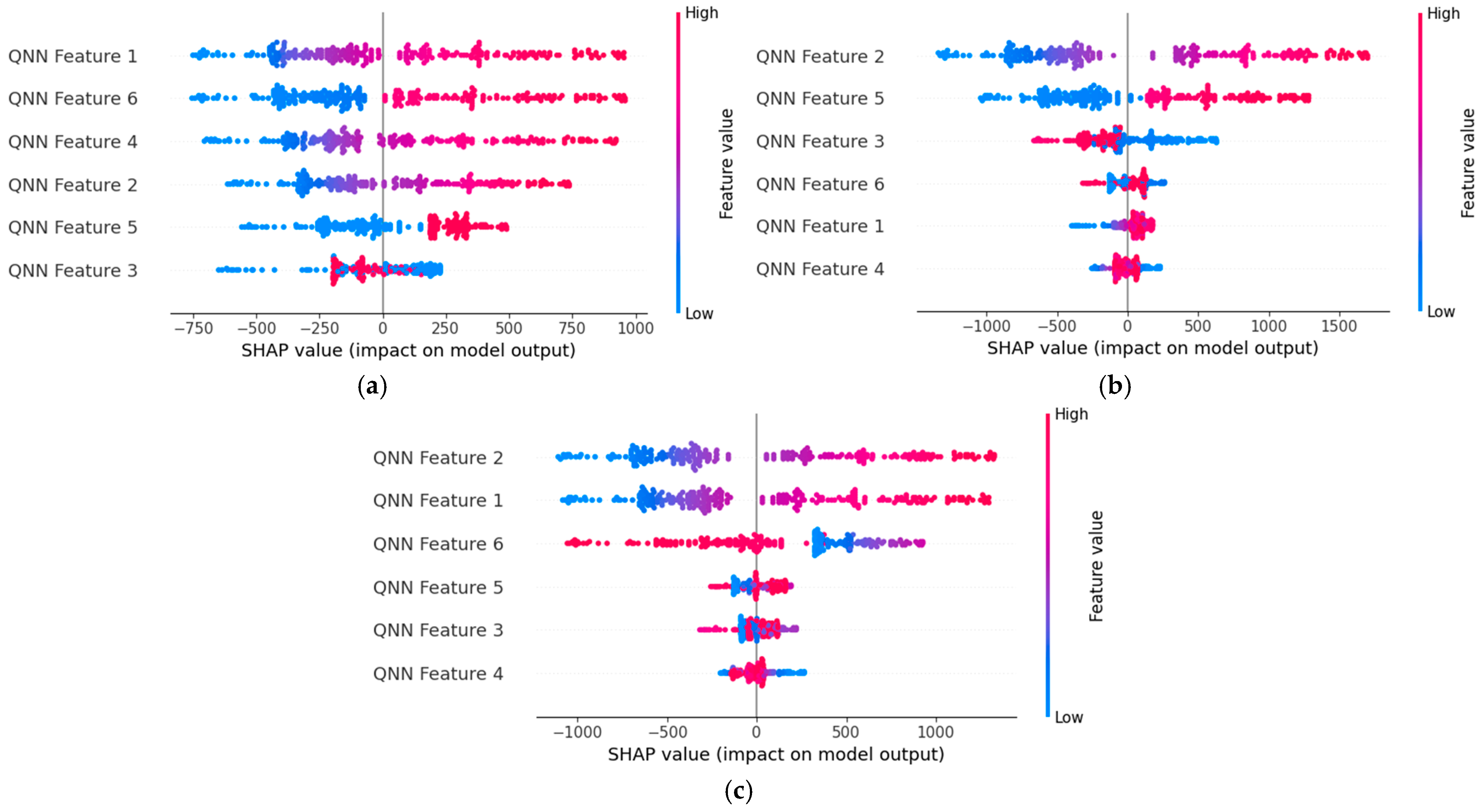
4.5. Explainability Analysis Using SHAP for Varying Fault Resistances and Noise Levels
To demonstrate the explainability and interpretability of the proposed QDNN-based method, SHAP was utilized to analyze the model’s behavior under different fault resistances and noise levels. The SHAP method quantifies the contribution of each feature to the fault location prediction by breaking down the overall prediction into individual feature impacts. This interpretability not only ensures the reliability of the model but also allows system operators to better understand how fault characteristics, such as TOA or polarity, influence the decision-making process. Additionally, the balanced distribution of SHAP values across features ensures that no single feature disproportionately influences the prediction, which is particularly important for avoiding overfitting in real-world scenarios.
The SHAP summary plots for the QDNN model, shown in
Figure 11, highlight how feature importance and impact vary across different fault resistances.
At 10 Ω fault resistance, shown in
Figure 11a, features like QNN Feature 2 and QNN Feature 6 exhibit the highest SHAP values, indicating their critical role in fault location prediction
. The SHAP summary plot reveals that these features significantly influence the model’s output, as their high SHAP values indicate a strong correlation between these features and the fault location results. The plot also demonstrates a balanced distribution of positive and negative SHAP values, showing that the model remains consistent and accurate at this fault resistance level. Importantly, the concentration of SHAP values around key features indicates that the model can effectively prioritize relevant factors over noise, ensuring robust predictions even under low-resistance conditions.
When the fault resistance increases to 50 Ω, as depicted in
Figure 11b, the model dynamically shifts its reliance on features. Here, QNN Feature 3 and QNN Feature 5 become more prominent, as evidenced by their increased SHAP values. This indicates the model’s adaptability in re-evaluating the importance of features under different resistance levels. Such behavior reflects a deep learning architecture capable of recognizing subtle changes in fault characteristics and recalibrating its predictive focus accordingly. The separation between high-impact and low-impact features is clearly visible in the SHAP plot, further demonstrating the model’s robustness. By dynamically adjusting its reliance on features, the model ensures that the fault location remains accurate and interpretable, even as the resistance level introduces complexity.
At the highest fault resistance of 100 Ω, shown in
Figure 11c, QNN Feature 4 demonstrates a crucial role in maintaining prediction accuracy under these extreme conditions. Although the SHAP plot for this feature indicates a relatively smaller range of values, its consistent importance in the model’s decision-making highlights its resilience and critical role in extracting key fault characteristics. The SHAP values for this feature indicate its critical importance in driving accurate predictions under high-resistance conditions. The SHAP plot at this resistance level shows a wider range of values, which could suggest increased variability in the input–output relationship due to the challenging fault scenario. However, the model maintains a clear prioritization of key features, as evidenced by the consistent dominance of QNN Feature 4. This behavior underscores the model’s resilience and its ability to extract meaningful patterns, even under extreme conditions.
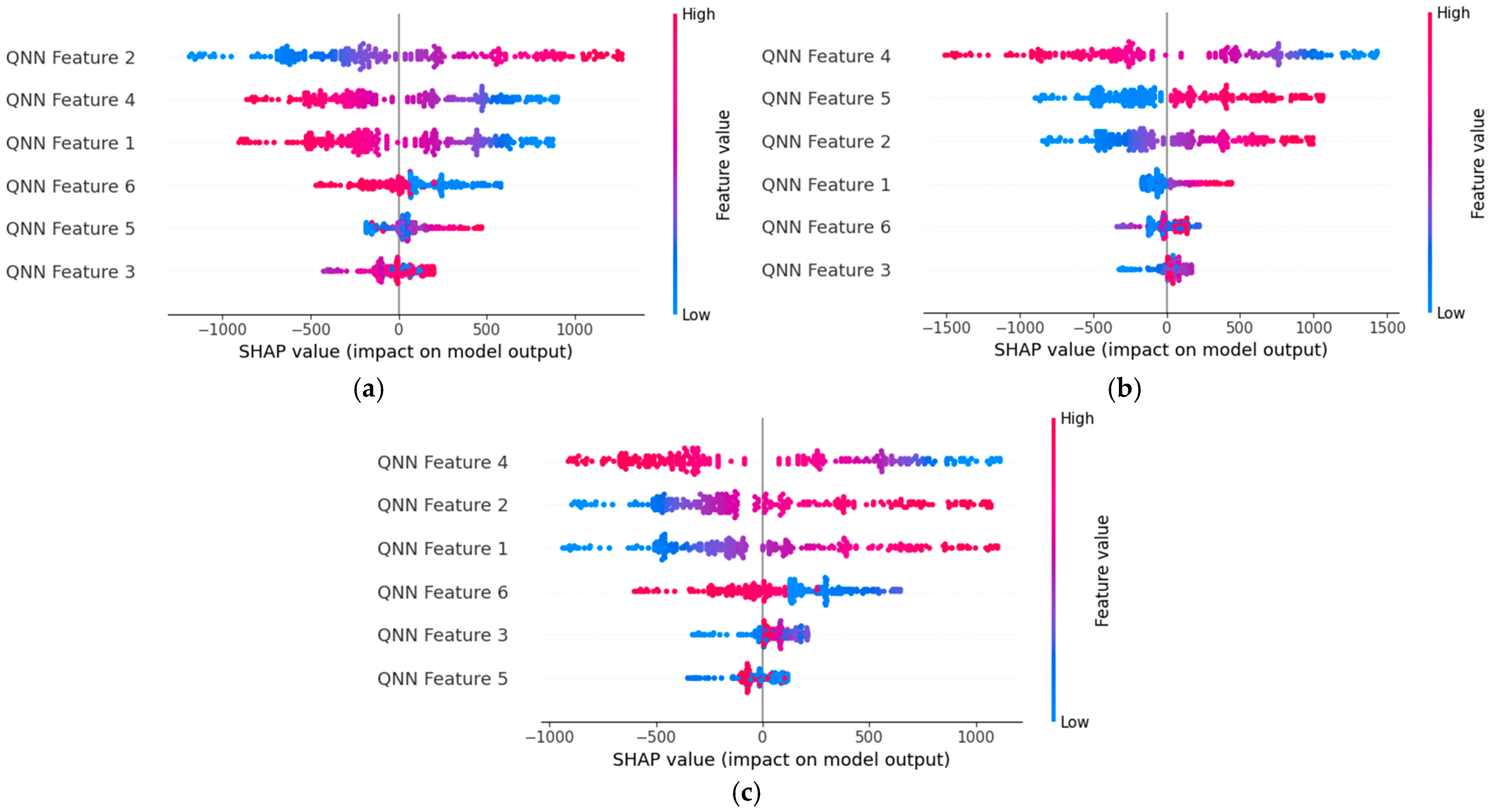
To further enhance the transparency and applicability of our proposed QDNN-based fault location framework, we incorporated it to provide detailed insights into the feature contributions under varying noise levels. In this study, fault scenarios under three distinct SNR levels were simulated. The SHAP summary plots, shown in
Figure 12, were utilized to analyze the impact of noise on the contribution of individual features within the QDNN model. These features, derived from the QNN architecture, include critical temporal and spatial parameters extracted for fault detection and localization. At low SNR levels, like 5 and 10 dB illustrated in
Figure 12a,b, the SHAP values demonstrate a higher variance, reflecting the model’s adaptability to handling noisy inputs while maintaining reliable predictions. As the noise level decreases, as with 20 dB shown in
Figure 12c, the SHAP values become more concentrated, showing reduced uncertainty and a stronger alignment with the most influential features, such as QNN Feature 2 and QNN Feature 4. Across all SNR levels, the QDNN model consistently identifies the same key features as highly influential, showcasing its robustness and noise resilience. This detailed analysis validates the applicability of our method in real-world settings where noise is inevitable, emphasizing its capability to maintain transparency and interpretability under varying conditions.
5. Conclusions
This paper presented an innovative framework combining XAI with QDNN to address the persistent challenges in fault location within DCMGs. The proposed methodology integrated HOSST for TW detection, CNNs for local feature extraction, and QNNs for quantum-enhanced data representation. Additionally, the incorporation of BD-LSTM layers and attention mechanisms enabled effective capture and emphasis of critical temporal patterns in fault signals. The experimental results demonstrated the framework’s exceptional accuracy and robustness across diverse DCMG configurations and voltage levels. The QDNN approach consistently outperformed traditional and modern fault location methods, achieving superior metrics in RMSE, MAE, R2, TUS, WIA, and VAF across training, validation, and test datasets along with superiority in correlation plot, RROC curve, and AOC values; specifically, QDNN achieved an RMSE reduction of up to 78.5% compared to traditional methods such as RNN and SVR, demonstrating its ability to significantly minimize prediction errors. Additionally, the AOC values for QDNN were consistently the lowest across the training, validation, and test datasets. Furthermore, the inclusion of XAI techniques and SHAP analysis provided valuable insights into feature importance, enhancing model transparency and interpretability. By overcoming limitations such as sensitivity to noise, reliance on communication links, and the challenge of high-resistance faults, this study contributes a highly adaptable and efficient solution to DCMG fault detection and location. To validate the robustness of the proposed framework in real-world scenarios, we conducted additional experiments modeling practical challenges by evaluating the model’s performance under varying fault resistances and exploring the impact of noise levels on prediction accuracy, showing that QDNN remains stable even under high-resistance faults and high-noise conditions. These results highlight the proposed framework for hybrid AC/DC microgrids, power distribution networks, and other intelligent energy systems. By combining state-of-the-art quantum computing techniques with XAI, the proposed framework not only enhances fault localization accuracy but also offers unparalleled transparency. This dual focus ensures that the model can be seamlessly adopted in real-world systems, fostering greater trust and reliability among system operators. Future research could focus on optimizing the quantum circuit design and expanding the dataset to further validate the framework under broader operational scenarios.


