Abstract
Electric vehicle (EV) emissions occur when a vehicle is charged and are based on the mix of power sources used during that period. The rapid growth of solar and wind energy has introduced a high degree of variability in the emissions of the grid for both diurnal and annual periodicities. Growth in solar energy has been particularly prominent in California. Using grid mix data spanning April 2018 to April 2023 from the California Independent System Operator (CAISO) and power source emission factors, we evaluate the grid mix at 5 min intervals and estimate the emission factors based on the mix of power sources, the transmission losses, and the AC/DC conversion. We compare the emission factors derived from this analysis to other static factors that can be used for estimating EV emissions. We find that, when using Low Carbon Fuel Standard (LCFS) emission factors, the average emissions rate was 301 g CO2-e per kWh over five years. However, depending on the time of year, the maximum hourly grid emission factors in California can be between 50% and 300% higher than the minimum factors. This difference suggests that the accurate measurement of emissions from electric vehicles would be improved with better data characterizing energy by the time of day and year in which the vehicle was charged.
1. Introduction
Electric vehicle (EV) production and ownership have expanded considerably during the last decade. It is well established that EVs provide a critical pathway to reduce greenhouse gas (GHG) emissions from transportation systems. In California, transportation represents about 37% of all GHG emissions, much of which is derived from vehicles powered by petroleum [1]. As a result, the state has sought to establish several policies that seek to accelerate the transition of the vehicle fleet away from petroleum consumption. These policies include Executive Order N-79-20, which states that “100 percent of in-state sales of new passenger cars and trucks will be zero-emission by 2035” [2]. Many other policies seek to promote the deployment of EVs within transportation network company (TNC) fleets and public transit systems, build a charging infrastructure, and broaden the use of clean power sources.
Despite these policies, challenges remain with respect to lowering the charging times, expanding charger availability, and increasing low-carbon electricity generation, among other issues [3]. Wrapped within these challenges is the measurement of the impact of emissions resulting from the on-road use of EVs. Unlike ICEs, where the GHG emissions from fuel combustion are generally the same at all times of the day and year, the emissions associated with EVs can change depending on when and where they are charged. This variability exists not only over the course of a single day but also over the course of the year. The variability in emission impacts has only increased with the expansion of renewable energy sources that feed electrical grids, most notably solar power, which varies both diurnally and annually. The purpose of this paper is to quantify how this variation has influenced EV emission factors in recent years.
The increasing variability of emissions from electricity production is evident within the state of California, where the use of wind power and solar power have greatly increased over the last decade. In 2023, solar photovoltaic (PV) and solar thermal power plants generated more than 41,000 Gigawatt hours (GWh) of energy compared to just 854 GWh in 2009, a growth of 4800%. Wind power generated around 13,920 GWh of energy in 2023, more than double the 6249 GWh reported in 2009 [4]. The expansion and variability of these power sources has implications for energy use and the associated emissions at any given time. Those implications have also changed relatively recently. In the first decade of the 21st century, the variability of electric grid emissions was not subject to large periodic changes in solar and wind power.
During and before this period, the emissions from electrical energy use at night could be even considered cleaner than daytime emissions. This was because fossil-fuel burning peaking (or peaker) power plants, which supplement the electricity supply during times of peak electricity demand, operate at lower efficiencies relative to the base load power. They are most commonly run during the day when there are large demands on power [5]. Peaker plants are being replaced as battery storage and combined cycle plants are reducing the need for them. Peaker plants can run for just 10% of a year [6]. However, in California at present, the large baseload delivered by solar has flipped this dynamic, yielding cleaner emissions from production during the day relative to the night. California now commonly deals with the issue of “renewable energy curtailment”, when, at certain times of the day and year, the state has too much energy from renewable sources. In response, the state reduces its output from these sources when there is not enough power demand to consume them. These events happen throughout the year, but are most common during the summer months when solar power is most abundant [7]. Naturally, such events are also highly variable depending on changing conditions related to wind and state-wide cloud cover.
This new dynamic, which largely emerged during the previous decade, has implications for measurements of EV emissions. Large variations in the hourly and yearly sources of power generation in electric grids require emission factors that are more precise regarding the time of day and year as well as the actual charging time as opposed to time of vehicle use. In California, EVs that charge during summer days have vastly different emission factors than those charging during winter nights. This paper addressed questions related to how the recent power source distribution of the California electrical grid translates into average emission factors and how those factors vary over the day and year. We use grid mix data published by the California Independent System Operator (CAISO) and power source-specific factors for each type of generation. We present the time-specific emission factors derived from both lifecycle assessment (LCA) and instantaneous emission factors.
The emission factors are tailored to charging EVs and adjust for transmission losses and the conversion of AC to DC. The analysis also explores the differences in factors that arise when LCA (plant construction, material manufacturing, etc.) are used versus instantaneous factors (e.g., directly from fuel combustion). Broadly, the study quantifies the relative magnitude of the differences in emission factors associated with charging an EV in California throughout the year and during different times of day. We compare these emission factors with similar flat factors, those that do not vary over time, to show the relative differences in measurement when the grid mix over time is considered. In the sections that follow, we provide background information on EV emissions and discuss relevant previous research. We follow this with a discussion of the data that were used and the methodology applied. We then proceed with a presentation of the results, including the calculation of the factors and a discussion of their dynamics during the day and over the course of the year. We conclude with a discussion of the implications of these findings for measuring emissions during EV charging and use.
2. Background and Previous Research
Transportation is among the largest end-use sectors of GHGs within the US economy. In 2019, the transportation sector had the highest (CO2) emissions in the nation, ahead of the industrial, residential, agricultural, and commercial sectors. Transportation was the second largest emitter of total GHG emissions, just behind the industrial sector, due to the latter’s high methane emissions [8]. GHG emissions from transportation have been stubbornly difficult to reduce. The main reason for this is the heavy reliance on petroleum and the limited choice of affordable, consumer-accepted electric vehicles or other vehicles using an alternative fuel source. However, this is changing, as EVs have grown considerably within the personal vehicle market. The expansion of the EV market has had strong government backing in many areas, as states including California have advanced policies to promote EVs and zero-emissions vehicles (ZEVs) [9].
The typical EV configuration is a battery–DC bus–inverter–motor. The batteries used in EVs can vary in their chemistry. Although lithium is the most common element and is currently used in various configurations, there are ongoing challenges related to battery management and health over time [10]. Additionally, end-of-life considerations are an area of active research as the impending retirement of early-market EVs will yield a stock of batteries that must be repurposed or recycled [11].
EVs have a well-known advantage over internal combustion engines (ICEs) with respect to their efficiency. They have an energy conversion efficiency of 95%, and their propulsion chain has an energy conversion efficiency of 77%. In contrast, most ICEs have a thermal efficiency of roughly 25% [12]. There are also other configurations, such as hydrogen fuel-cell hybrid electric vehicles (FCHEVs), which exhibit a high conversion efficiency and have emissions that are a function of the grid power sources and the efficiency of electrolysis [13]. However, regardless of the carrier fuel, EV emissions per mile are ultimately dictated by the source of the EV’s electric power and the EV emissions discussed in this paper are in the context of pure-battery plug-in EVs.
The differences between the drive trains as a function of electricity production and consumption have been previously documented. There is a difference in these impacts depending on whether lifecycle or in-use (instantaneous) emissions are considered. Hawkins et al. (2012) conducted an environmental impact assessment on both EV and ICE vehicles and presented a comparison regarding global warming potential, acidification potential, smog, and toxicity [14]. They reported that EV GHG emissions are heavily impacted by the use phase, and that well-documented lifecycle indices for EVs would be needed to estimate the environmental impact of the electricity required to charge a vehicle fleet [15].
EVs have long been thought of as an eventual source of supplemental battery capacity for the electrical grid. Kempton and Letendre (1997) studied the integration of EVs into the grid and determined that this could help reduce the need for base-load generation, reduce the time-of-day mismatch between generation and load and increase the receptivity of the grid to intermittent renewables [16]. More recent work has continued to expand on the concept of vehicle to grid integration, both in terms of technical implementation and the supporting business models [17]. Sovacool et al. (2020) evaluated perceptions of business models that would support V2G integration [18]. This need for a better understanding of the upstream emission factors derived from electricity production speaks to the challenge of estimating the emissions associated with EV charging with better precision.
The carbon intensity of electricity emissions in the US has fallen in the last fifteen years, with 2023 emissions being slightly below 60%, the level of 2005 [19]. However, despite the rapid increase in the use of solar and wind power within certain regional grids, the decrease in the carbon intensity of the broader American grid is mainly derived from the substitution of coal with natural gas [20]. In the US, the annual electricity generated from coal went from 1,733,430 thousand megawatt hours in 2011 down to 773,393 thousand megawatt hours in 2020, and the annual electricity generated from natural gas went from 1,013,689 thousand megawatt hours in 2011 to 1,626,790 thousand megawatt hours in 2020. At the same time, the generation capacity of solar and wind power saw exponential growth over the last decade, accounting for just over 10% of the total energy generation in the country by 2020. Hydroelectric and nuclear power have remained relatively flat [21].
This transition has implications for EV emissions. The report authored by McLaren et al. (2016) conducted an analysis of the anticipated emissions produced by battery electric vehicles (BEVs) and plug-in hybrid electric vehicles (PHEVs) [22]. The study assesses the impact of BEVs and PHEVs based on the marginal emissions associated with plug-in charging instead of the general grid profile, while accounting for the emissions associated with non-electrical miles (miles traveled using gasoline for PHEVs and miles traveled by BEV owners using a conventional vehicle due to a BEV’s limited range). The study simulated five emission profiles using the production cost model PLEXOS. McLaren et al. also calculated the electric loading caused by seven vehicle types under four charging scenarios. The Battery Lifetime Analysis and Simulation Tool for Vehicles was then used to incorporate behavioral tendency data into the simulation, and the emissions associated with charging were calculated using the non-lifecycle emission factors by Brinkman et al. (2015) [23]. A sensitivity analysis was conducted at the end of the report by replacing a percentage of the generation mix with a mix containing higher/lower coal and natural gas usage. The report concluded that the grid electricity carbon intensity has a greater impact on the emission reduction potential than the charging scenarios, and PHEVs had higher emission reduction potential when considering the non-electric vehicle miles traveled. The report also concluded that the availability of workplace charging could lead to more electric miles, thereby providing the highest potential for emissions reductions for both BEVs and PHEVs.
Many areas within the United States saw a recent decline in their per-unit carbon intensity of electricity. The State of Texas is one example. As shown by Zhang et al. (2024), the emissions from electricity generation in Texas have been in decline since 2020 due to the replacement of coal with natural gas and wind. Natural gas and wind generation can provide power at all times of the day [24]. California, in contrast, is able to generate a large share of its electricity with solar power. The natural diurnal and annual availability of solar makes the state more vulnerable to mismatches in power demand versus supply. Hence, the emission factors of an electric grid are regional-specific, where the dynamics in one region may not translate to another.
This and other analyses have highlighted an important element of emission estimates, which is the difference between the average emission factors (AEF), which are the total electricity emissions divided by the total electric energy generated and the marginal emission factors (MEFs), which measures the emissions per unit of the extra electricity generated due to some additional load.
The AEF and MEF can be different, and some have reported that if the MEF is significantly larger than the AEF, the emission reduction potential of EV implementation could be overestimated. Holland et al. (2022) estimated the marginal CO2 emissions derived from US electricity generation using the recent data and concluded that the MEF of the United States increased by 7% despite the 28% decrease in AEF over the last decade [25]. The MEF also varies from area to area. Siler-Evans et al. (2012) used hourly generation and emissions data from 2006 through 2011 to construct a regression model and conducted a systematic calculation of the MEF of the United States. The authors discovered significant regional differences in emissions showing the benefits of avoiding the use of a unit of electricity [26]. For a grid that is served by a relatively consistent baseload and peaker plants, the MEFs represent the emission factors of the peaker plants supporting the additional load. However, MEFs can be complicated by the fact that renewable resources are regularly in flux due to the large daily changes in wind power and solar power, which can be difficult to predict. The time of day also matters due to the current dominance of solar power in California, and Holland et al. (2022) show that MEFs do decline during the day [25].
As noted earlier, California currently faces the challenge of having an oversupply of renewable energy during certain times of the day and year. This oversupply is curtailed by reducing the output from solar and wind, while other renewable sources, such as small hydroelectric, geothermal, and bio-based resources, are generally not reduced during times of oversupply [7]. Natural gas use does drop on a daily basis, corresponding to a rise in solar power, but it does not reduce to zero. Curtailment data from the California Independent System Operator (CAISO) suggest that, in 2022, 2449 GWh of solar and wind electricity was curtailed due to a lack of demand during the times at which they were available. While most curtailment does occur during daylight hours, curtailment happens every month of the year. In 2022, 17% of the curtailed energy was curtailed between November and February [27]. Ryan et al. (2016) presents a good discussion and review of the many different approaches used for calculating emission factors that have been applied to EV emission measurements, including AEF and MEF applications [28].
More recently, a report by the National Academies discusses the different circumstances in which such factors are deployed in EV emission measurements [29]. The report recommends that AEFs are applied in attributional LCA, where measurement of the emission impacts of a process is of interest. For example, evaluations that are measuring the GHG emissions of an EV that was already driven in a TNC or ridehailing service, a carsharing system (offering short-term access to a shared vehicle), or a personal vehicle within a grid of a known mix would be best measured by AEFs. The report recommends the application of MEFs for consequential LCAs, where the system being measured changes the grid mix itself. For example, modeling the introduction of EVs into the broader personal vehicle fleet of a state would have an impact that is large enough to require the grid to adjust its mix of power sources to handle the new load. In this case, MEFs may more appropriately capture the total impact of the new load and the adjustment that the grid makes to handle it.
The same calculation could be carried out using the new AEFs on the load and the difference in the AEFs on the rest of the grid, both pre-load and post-load. This calculation is more reflective of the new load; the AEFs are increased for everything, and more emission-intensive power was distributed across the entire grid. However, calculating the impact in this way requires knowledge of the load of the broader grid, whereas using MEFs only requires knowledge of the new load being modeled. In this way, MEFs are effective. However, the application of MEFs to an exercise should consider the value judgment that they imply. That is, MEFs imply that the modeled load often leads to more carbon-intensive emissions. But those higher MEFs are equally caused by all the other loads also on the grid. Because these loads are present, they support elevating the MEFs to their more carbon-intensive values.
Numerically, MEFs accurately capture the change in impact, but in terms of policy discussion, they can be interpreted to imply that the modeled load is the exclusive cause of the increase in emissions when the broader set of loads on the grid (lights, appliances, etc.) are also pushing the factors higher and are turned off and on just as much. Both types of factors have appropriate applications. To support the evaluation of EV deployments for specific projects and use cases, we explore the magnitude and variance of AEFs, as derived from different types of emission factors and the empirical data on the grid mix for California from April 2018 to April 2023.
3. Materials and Methods
This study applies California grid mix data at a temporal resolution of 5 min intervals to several types of emission factors. The calculation of an AEF is effectively a sum-product calculation, where the percentage that the grid is supplied by each discrete power source is multiplied by a factor that describes the GHG emissions per unit of energy from that power source. The sum of these products produces the AEF for the given time interval. To account for EV charging applications, additional scalers are applied to adjust for transmission losses and for the conversion of AC to DC for battery storage.
A main source of the data for this study is the publicly available grid mix information of the CAISO; this shows the percentage of power sources at 5 min increments from 2018 to 2023. CAISO reports the daily pattern of the grid mix for California’s power grid, along with the composition of the total electricity derived from renewable sources. The time series of these grid mixes can provide an insight into the magnitude of the variability of emission factors that could apply to EV charging at different times of the day and year. An analysis of these data was used to compare the variability in the grid emissions to the average, as well as to other emission factors that would be applied in a conventional calculation of emissions that occurs from EV use.
There are several types of emission factors that can be used to generate emission estimates. One type is lifecycle emission factors (noted earlier as LCA), while another type is instantaneous emission factors. The LCA considers the full implications of emissions from electricity generation. The system boundary extends beyond fuel-burning, and encompasses the production of fuel, the construction/operation of the facility, and disposal. The LCA factors are almost never zero, as even renewable power sources require the manufacture of materials and infrastructure to produce power without burning fuel. The LCA factors applied in this paper were extracted from Horvath and Stokes (2011) [30]. Instantaneous emission factors are those that consider only emissions from fuel combustion to produce power. These factors ignore any emissions from resource extraction, equipment manufacturing, or disposal connected to power production. The instantaneous factors applied in this paper are derived from the Low Carbon Fuel Standard (LCFS), regulated by the California Air Resources Board (CARB).
To translate the grid mix percentages to grid emissions, we explore the application of both types of factors to illustrate their differences in the context of EV charging. All sources of lifecycle emission factors, except for hydropower, were derived from Tables 5-1 of Stokes and Horvath (2011) [30]. The emission factors for large and small sources of hydropower were drawn from the results of Kadiyala et al. (2016) [31], which summarized the lifecycle emission factors of various LCAs of hydropower to derive the mean factors of hydropower generation for plants of various sizes. The lifecycle emission factors were 40.63 gCO2eq/kWh for large hydropower sources and 21.05 gCO2eq/kWh for small hydropower sources.
California’s grid mix also includes a component called “imports”, which consists of electricity generated from outside the state. Imports fluctuate considerably over the day and year and, due to their nature, are themselves a function of a grid mix. The emissions factor of natural gas lies in the midpoint between renewable and non-renewable sources, and more than 40% of the American grid runs on natural gas [32]. In the absence of more precise measurements, the emission factors related to imports were considered to be the same as those of natural gas. We validated this assumption by running an ordinary least squares (OLS) regression model on the carbon intensity of the CAISO grid, which served as the dependent variable on 60 randomly selected days within the dataset, with the percentage of power sources as the independent variable. The coefficients of the natural gas and imports were found to be close to each other for each model (on average 0.6%). The models were collectively found to have an adjusted-R2 of 0.97 or above. This validated the assumption that the reported imports within the CAISO grid were predominantly considered to be derived from natural gas power sources.
It is worth noting that most organizations and models use their own set of emission factors. In many cases, the emissions resulting from combustion alone, instead of lifecycle emission factors, are used. For example, the Energy Information Administration reports 53 kg CO2/million British Thermal Unit (btu) as the emissions factor for natural gas and 71 kg CO2/million btu for gasoline. However, it considers renewable sources such as hydro, wind, and solar as having no carbon emissions [33,34].
In addition to the emissions from electricity generation, energy is lost with grid transmission and AC-to-DC conversion. Stokes and Horvath reported that the average grid loss is around 10% in the United States. For hydropower generation, the system boundary of the LCA varies from study to study, but generally covers the emissions embedded in the construction and operation of the plant. The lifecycle assessment of hydropower generation did not include grid loss, with an exception being site specific-studies of micro-hydropower plants. Therefore, to account for the grid loss and the energy loss involved in AC-to-DC conversion, loss factors were applied. According to Deru and Torcellini (2007), the average grid loss in the Western grid was 8.4% [35]. The energy loss involved in AC-to-DC conversion can be assumed to range from 10% to 15% [36].
Lifecyle factors are especially useful for evaluating emissions related to the outside impacts of a power source, which may not be associated with its use but occur because of its existence. It is relevant to understand these emission factors as separate from those derived from instantaneous power sources. These factors consist of those that are aligned with the impacts of the use of specific power sources. For example, the lifecycle emission factors of solar energy suggest that some emissions may be derived from solar power, but these are mostly a result of the production and disposal of solar panels. However, the production of a kWh of solar power is emissions-free and, in many situations, 0 gCO2e/kWh is the appropriate factor to use. Instantaneous emission factors are often used in policymaking and emission calculations, particularly when an investment in the necessary infrastructure has already been made. The LCFS policy adopted by CARB, for example, applies instantaneous emission factors for its calculations of electric fuel use. Those factors, as well as the lifecycle factors assembled for this study, are shown in Table 1 [37]:

Table 1.
Instantaneous and lifecycle and emission factors.
The calculation of the EV emissions factor per kWH for a given hour during a given month is a function of (1) the percentage of power supplied a given source, (2) the power source emissions factor, (3) the efficiency losses associated with transmission, and (4) the efficiency losses associated with converting the delivered AC power to DC. A generalized representation of this calculation is presented graphically in Figure 1.
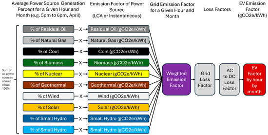
Figure 1.
Graphical representation of factor calculation.
Note that the output of this calculation provides emission factors in units of (gCO2e/kWh). However, the final step in estimating the emissions from a specific vehicle requires knowledge of the vehicle’s efficiency per mile (kWh/mile), just as gasoline vehicle emissions require knowledge of the miles per gallon (mpg). This last step is left to the analyst applying these factors to a specific vehicle application, which can be done in several ways.
In the section that follows, we present the results of an analysis of the trends in power sources during the period of study. The results show the degree to which the intensity of emissions varies over the course of the day and year within a grid that has a relatively large share of renewable energy production led by solar. We further compare life-cycle-derived versus instantaneously derived emission factors and compare them to other available factors to estimate the emissions from electric vehicles. There are some limitations to the analysis. Notably, this analysis only calculates AEFs, which are most suitable for applications in attributional LCAs, for measurements of EV emissions that have already occurred or for near-future EV emissions that are small enough to not significantly influence the grid load. The California grid is likely to change and so the AEFs presented here will inevitably become dated with time. For example, should power demand rapidly outpace the growth of renewable energy sources, the AEFs would increase as the demand would be served by fossil fuels. The periodic recalculation of AEFs is recommended to ensure the accuracy of emission estimates, particularly if the grid of the future is subject to major changes in the levels of demand or the mix of power sources relative to the California grid at present.
Our analysis shows that the mix was relatively stable over the course of the five years studied. Some of the factor tables are similar in structure and content to those produced for California LCFS Lookup Table Pathways, but with a monthly resolution and a supporting longitudinal analysis of the AEFs and variance [37]. We further offer comparisons of these factors with flat time-independent factors that are also available for application to EV emissions. Additionally, the factors presented are a function of the correctness of the input factors specific to the individual power sources that supply the grid. Variations in assumptions regarding these power factors would influence the outputs presented in this study. Overall, the findings have implications for the understanding of the measurement of the emission impacts from EV systems and the electric charging policy within California and may inform the structure of similar analyses within other regional grids.
4. Results
The results show that factors governing emissions from electricity in California exhibit considerable temporal variability. This is driven by the variations in the availability of specific resources generating power. The largest diurnal variations are with the availability of sun and wind. Taken together, the continuous variations in power sources influence the carbon intensity of the electricity generated over time. The magnitude of these variations has direct implications for the net emissions that result from charging EVs at different times of the day.
To present an example of the size of these variations in power sources across the course of a single day, Figure 2 shows a plot generated by the authors of the CAISO data revealing a mix of power sources being used during a single day, 15 March 2020. The largest change in the power mix occurred with the rise in solar power during the day, which was commensurate with a drop in the use of natural gas and, to a lesser extent, imports from the interstate western electrical grid. As noted earlier, imports are aligned with the emissions rate of natural gas, but can consist of a diverse array of renewable and non-renewable power sources, including the generation of coal. Very little (57 MW) coal power is generated within California [9].
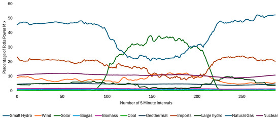
Figure 2.
Sample daily percentage of each variation in energy source on 15 March 2020.
The combination of shifting power sources during the day yields a shifting net emissions factor that can be assigned to EV charging during the day. The magnitude of this variation in LCA-based emission factors is shown in Figure 3 for the same day, 15 March 2020, as an example also generated by the authors. The notable surge in solar and wind power during the day causes a commensurate decline in the generation of power from natural gas and electricity imports. This diurnal pattern of power sources causes the estimated net emissions factor to swing by almost 50%, where energy used during the midday solar and wind peak is about half as intensive in terms of emissions as the energy consumed during the early morning and evening. The magnitude of the changes that occur during a single day motivates the need to obtain a better understanding of the combined emission factors over time to estimate the emission-based impacts of EV charging. The application of a flat average factor to estimate EV emissions via a VMT or a kWh conversion factor would over- or underestimate the impact of charging depending on the time of day in which the charging occurred.
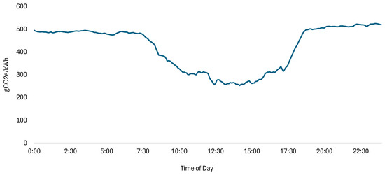
Figure 3.
Sample daily LCA-based emission factor for 15 March 2020.
Just as significant variation was observed within the course of a selected day, variations in emission factors also occur over the course of the year. The natural variations in solar insolence, as well as the variation in wind and hydroelectric power availability over the course of the year, impacts the emission factors derived from EV charging at different times of the year. Figure 4 shows a plot of the emission factors for each day within the dataset, overlayed with all other days. Every line represents a day and the emissions factor at a given time of that day. Figure 4 presents the complete distribution of the carbon intensity of the power generated in California for each day within the entire period covered by the dataset, from April 2018 to April 2023, based on LCA-based emission factors.
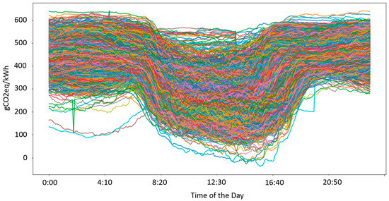
Figure 4.
Daily net LCA-based emission factor variance, (with each line signifying the pattern for each individual day).
Figure 4 shows that during the five-year period, the LCA-based net grid emission factors can span anywhere between approximately 0 gCO2/kWh to about 650 gCO2/kWh. There is a greater variability in emission factors during the middle of the day. These emission factors can be summarized into an average and standard deviation for each hour over time. This is shown in Figure 5, where the average emissions rates by hour and the standard deviation are both plotted. The figure shows that across the three-year period, the average LCA-based emissions rate during the day varied from 484 gCO2e per kWh over night to about 292 gCO2e per kWh during the middle of the day. These averages, which represent a five-minute interval, show a variation that increases during the middle of the day. The higher variation that is found during midday is mainly driven by variations in solar power over the course of the day.
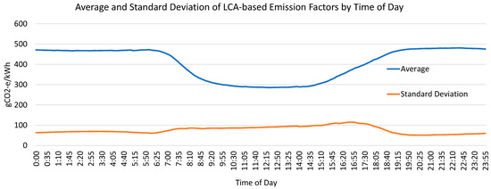
Figure 5.
Average and standard deviation of LCA-based emissions over the course of a day.
As the mix of power sources changes over the course of each year, so does the relative mix over time. The daily profile of average LCA-based emission factors for each month is shown in Figure 6. For simplicity, these plots show the average of the same month over the course of multiple years recorded in the dataset. The same pattern persists throughout the year, where solar power reduces the emission factors to their minimum during the day, even in December. However, even though the emission factors are always at their minimum during daylight, the monthly comparison shows that the magnitude of those minimums can vary significantly. Notably, the midday emission factors for the months of April and May are almost half those in November or December. This large variation during the year and during the day emphasizes the need to consider time-dependent emission factors at the time of charging as the power sources supplying the grid continue to diversify with a greater share of renewable resources.
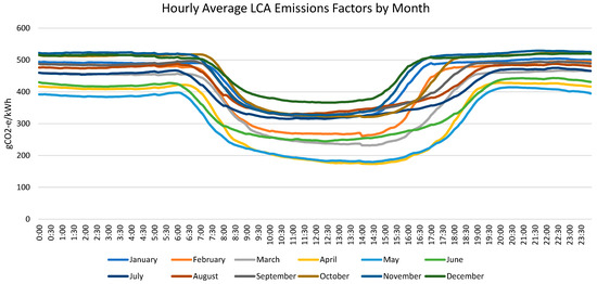
Figure 6.
Hourly average LCA-based emission factor by month (2018 to 2023).
The natural variation shown in Figure 6 translates to a variation in the monthly average factors. These are shown in Figure 7, where the undulation over the years reveals minimum average emission factors that consistently occur during May. The reason for this is due to a combination of events. Notably, hydropower increases seasonally in the state, from March to May, because of the Sierra Nevada snow melt. This, combined with the increasing daylight available for solar power, means that the state’s minimum electricity emission factors presently occur in mid-to-late spring. Figure 7 also presents a plot of the standard deviation of emission factors over the course of the dataset. Unlike the daily standard deviation, the monthly series shows less of a clear cyclical pattern. However, the annual peak variation regularly occurs in the spring, either in March or April, which is again likely connected to the unique power-generation dynamics of this season.
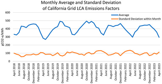
Figure 7.
Monthly average LCA-based emission factors (2018 to 2023).
Figure 8 shows a plot of the percentage of power derived from each primary source. Solar power (hollow blue line) unsurprisingly reaches maximum rates in June, but it is the increase in other supporting renewable power sources that makes May the month with the lowest emissions. Also influencing these emission factors is power demand, which rises considerably during the summer and is met by natural gas (dashed line). That is, there is a grid demand side of the equation that is also influential regarding net emission factors. The plot shows that natural gas was the dominant power supply during the five-year period. Natural gas and imports (dotted line) were heavily relied on during the winter months. This reliance falls considerably during late spring with seasonal increases in large hydro, solar, and wind power. Also evident from Figure 8 is the strong and steady role that imports play throughout the year. Notably, the use of imports increases during periods with natural declines in solar power, although this pattern appears to break in the final year of the dataset. This appears to be because in-state natural gas could better meet the demand than in previous years.
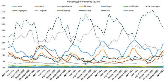
Figure 8.
Percentage of power from each source (April 2018 to April 2023).
The seasonal oscillation in each of these power sources influences the emissions derived from electricity. Figure 7 and Figure 8 show that, at least from April 2018 to April 2023, the patterns in power production and emission factors were relatively stable. There were notably higher peaks in solar and wind power each year, but these changes occurred gradually. Solar power peaked at 16.7% of total power in 2018 and 22.6% of total power in 2022. The implications of the variations in power sources are critical to managing the charging of vehicles as well as other energy demands. Based on the 5-year dataset and the power source emission factors applied previously, the 5-year average LCA-based emission factors for electrical energy are shown in Table 2. These factors include an efficiency adjustment of 8.7% for transmission losses [35], as well as 15% for converting AC to DC energy.
Table 2.
Cross tabulation of average California emission factors (gCO2/kWh), calculated using LCA-based factors by month by hour (April 2018 to April 2023).
Table 2 shows the wide variation in factors that occur because of the fluctuating power sources. The minimum average factor of 223.6 gCO2/kWh occurs during the 2 pm hour in April. The maximum factor of 678.1 gCO2/kWh occurs during the 9 pm hour in November, which is almost three times the minimum average factor. The average across all these factors is 528 gCO2/kWh. The factors within Table 2 depend heavily on the emissions rates assumed for each power source. For these factors, each power source has an emissions rate that is dictated by lifecycle emissions that include both “in-use” (instantaneous) emissions and the upstream emissions associated with the production and operation of the power source. When comparing these factors to other fuel sources (e.g., gasoline), the LCA-based factors of petroleum fuel should also be considered. Such factors not only account for the combustion of the fuel, but for the upstream mining, production, and distribution of the energy required to deliver it.
Different assumptions regarding the system boundary will yield different average emission factors. For example, CAISO also calculates emissions rates regarding its power consumption and tracks these emission estimates in real time. The assumptions made in these calculations are different from those made for the factors discussed above and are derived from the CARB GHG Emissions Inventory Data [1]. Such factors apply to instantaneous emissions and only to certain sources, where such emissions are relevant (e.g., combustion emissions). For these types of factors, sources that involve no major emissions-producing power, such as solar power, wind power, nuclear power, and hydropower, are considered to have zero CO2 emissions. The accuracy of a zero-emissions factor for these power sources depends in part on the objective of the measurement. If the objective of the measurement is to assess emissions after the construction of the power sources, then a zero-emissions factor can be justified for those resources that do not combust fuel. LCA-based factors consider the one-time production/construction emissions that are amortized over the lifespan of the product. Understanding LCA-based factors is essential for decision making in long-term investments, where technologies that achieve zero instantaneous emissions but produce high emissions during the construction or deconstruction of the power source can mask their true impact relative to their in-use emission factors. California’s LCFS assigns zero emissions to non-carbon sources of power. Table 3 shows what the 5-year average factors would appear to be in this analysis when considering only power sources with instantaneous emission factors. These factors are consistent with the CAISO factors that are derived from CARB’s GHG Emissions Inventory and applied to the LCFS. The application of these factors to the grid mix, combined with the use of additional scalers to account for the transmission losses (8.7%) and AC/DC conversion (15%), are shown in Table 3, while their distribution is shown in Figure 9.
Table 3.
Cross tabulation of average California emission factors (gCO2/kWh) using LCFS-based instantaneous factors by month and by hour with estimated transmission and AC/DC losses (April 2018 to April 2023).
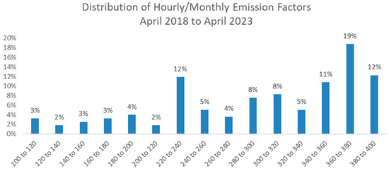
Figure 9.
Distribution of the instantaneous LCFS-based emission factors shown in Table 3.
The average emissions rate across all these values is 301 g CO2-e per kWh, with a minimum rate of 106 g CO2-e/kWh and a maximum rate of 406 g CO2-e/kWh. This maximum is 35% above the average, while the minimum is 65% below the average. As shown in Figure 9, the distribution of emission factors is negatively skewed, with 42% of the emission factors being 340 g CO2-e/kWh (13%), or higher than the average.
The factors in Table 3 are averaged over 5 years of grid mix data. During this time, weather and load variations, as well as changes in the sources of power generation (e.g., increasing solar and wind), will lead to variations from year to year (as shown in Figure 8). For example, due to the increase in solar production capacity, the grid mix from April 2018 to April 2019 may not be the same as the grid mix from April 2022 to April 2023. Such differences can be significant when studying rapidly changing grids. At the same time, the increase in power demands requiring the use of natural gas, or a reduction in output from low-carbon sources such as hydropower, wind power, or solar power can cause emission factors to rise even when the capacity for low-carbon power production expands. Figure 10 provides an insight into this fluctuation in the average, which relatively speaking, is not large. The final year presented in the data (April 2022 to April 2023) has the second lowest average emissions factor, while the period from April 2019 to April 2020 has the lowest. The highest average emissions factor across the five years is found in the third year. The upper bound of the emission factors within each year fluctuates as well, while the lower bound monotonically decreased during the 5-year period. Figure 9 shows that although the emission factors are generally stable, the most recent year may not necessarily be the lowest-emission year due to the dynamics explained above.
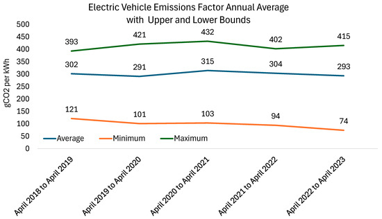
Figure 10.
Minimum, maximum, and average LCFS-based emission factors by year.
Analyses of emissions derived from EV charging should always use the factors that are most closely related to the time frame being measured. But Figure 10 shows that, even in a changing grid, multi-year averages can smooth out the variations that can occur with changes in the grid mix and under exogenous conditions. The time series shown in Figure 7 and Figure 10 exhibits a stationary trend. Overall, the stability of the time series suggests that the averages of these grid mixes will move slowly. Hence, multi-year averages can still represent the appropriate range and magnitude when generic factors are needed or updated data are not available.
The hourly and monthly emission factors presented above reveal the considerable hourly and monthly variations that occur when all other assumptions are the same. It is also useful to draw a comparison with the emission factors that could be derived from a few examples of conventional measurements of EV emissions. One example of this is the US Environmental Protection Agency (EPA) factor of miles per gallon equivalent (MPGe), which translates the effective equivalence of EV fuel efficiency to that of gasoline. The EPA defines MPGe according to the energy equivalence 33.7 kWh per gallon of gasoline. An MPGe of 132 means that an EV uses 33.7 kWh to travel 132 miles. The purpose of the MPGe is to present consumers with a means to compare the relative fuel efficiency of EVs to an MPG. However, because the denominator in this comparison is equivalent to a gallon of gasoline, this translation could be mistakenly interpreted as an emissions rate that is connected to the combustion of a gallon of gasoline. This interpretation would be incorrect because MPGe is based on energy equivalency and the efficiency of the vehicle in converting the energy into miles driven. It makes no assumption about the carbon intensity of the 33.7 kWh. Approximately 8.887 kg of CO2 emissions are produced per gallon of combusted gasoline, and the emissions per mile measurement of a gasoline vehicle is strictly a function of the vehicle MPG [38]. For example, a vehicle with an MPG of 30 has an implied emissions rate of 0.29 CO2 per mile. An MPGe of 132 would imply 0.07 kg CO2-e per mile if gasoline equivalent emissions were assumed. If MPGe were connected to a gasoline-based emissions factor, given that 33.7 kWh is considered the gasoline gallon equivalent at an emissions rate of 8.887 kg CO2 per gallon, it would imply that the MPGe is equivalent to a grid emissions factor of 264 g CO2-e per kWh. This emissions rate is coincidentally not very different than the average emissions rate of 301 g CO2-e per kWh that we calculated from the LCFS-based factors in Table 2. But because the MPGe metric is based on energy equivalence and not on the carbon-equivalence of gasoline, it should not be used to estimate emissions from EVs without a grid-based emissions factor applied to it.
Flat emission factors have no variance over time regardless of the grid mix. The greater efficiency of the EV when using the same amount of energy allows these factors to compare favorably to the emissions rate of a traditional gasoline vehicle with lower efficiency. However, it will not reflect the changes to the emissions rate that are increasingly derived from low-carbon energy sources or from the charging that occurs at different times of day.
Another important element of these per kWh emissions rates is that translating them to an average g CO2-e per mile can produce different results depending on whether an MPGe-based equivalency of 33.7 kWh per gallon of gasoline is used versus an estimate based on the vehicle range and battery capacity. For example, for a 2021 Tesla Model 3 Standard Range Plus RWD, which has a listed 142 MPGe, 263-mile range, and a usable battery capacity of 50 kWh, two slightly different emissions rates per mile would be computed when using the same input data on the same car [39,40]. Taking our average input of 301 g CO2-e per kWh, multiplied by 33.7 kWh per gallon and divided by 142 MPGe, an emissions rate of 71 g CO2-e per mile is derived. This calculation is shown below in Equation (1).
The same emissions factor input (301 g CO2-e per kWh), multiplied by a vehicle battery capacity of 50 kWh and divided by a range of 263 miles, will yield an emissions rate of 57 g CO2-e per mile, which is within the same relative magnitude of the previous estimate, but 20% lower. This calculation is shown below in Equation (2).
Even using the same emission intensity for the input energy can yield different per-mile emission rates within the same car. One method relies on the estimate of MPGe, while the other relies on the estimate of the vehicle’s nameplate range at full battery capacity. Both are estimates that are subject to uncertainty and change over time. One difference contributing to these discrepancies is that the MPGe estimate considers wall-to-battery charging losses, whereas the battery capacity equation does not consider this loss.
Another tool for estimating emissions has been available through the Department of Energy (DOE)’s Alternative Fuel Data Center [41]. This online calculator provides average state-specific measures of EV emissions relative to hybrid, plug-in hybrid, and EVs. Based on the U.S. Energy Information Administration (EIA)-derived assumptions from the 2021 grid mix and average driving patterns, the calculator effectively reported an emissions rate of about 208 g CO2/kWh for California and 397 g CO2/kWh for the nation. This California average is on the low side of the estimates presented in this study, but within their overall range. The differences could be due to different assumptions regarding the power-supply factors and the average time frame. However, even if this value was considered the true average within Table 3, the emissions factor could be as much as 51% or 195% of the average value depending on the hour and month in which the charging occurred.
Finally, it is worth noting that all these emission factors continue to show that EVs yield emissions per mile that are far lower than those of current gasoline vehicles or hybrid vehicles. The 5-year average LCFS-based emissions rate of 301 g CO2/kWh at 33.7 kWh per gallon translates to 10,140 g CO2-e per gasoline gallon equivalent, which is more than the 8887 g CO2/gallon emitted through the combustion of a gallon of gasoline. However, the high efficiencies of the EVs more than make up for this difference. When comparing an EV mpg-e of 132 versus a gasoline vehicle achieving 30 mpg, the EV will achieve an emissions per mile result of 77 g per mile versus 296 g per mile. Hence, the EV in this comparison will have per-mile emissions that are about 75% lower than those of what would presently be considered a typical gasoline vehicle. When the gasoline vehicle being compared is a hybrid, such as the Toyota Prius at 57 mpg, the per-mile emissions of a 132 MPG-e EV are about 51% lower. Naturally, the exact reduction depends on the emission factors and efficiencies being assumed, but with the average factors calculated this study, EVs are found to have lower emissions than typical gasoline and hybrid vehicles under almost all market MPGs and charging times, regardless of whether LCFS or LCA factors are used.
Overall, the evaluation of LCFS-emission factors and LCA-based emission factors suggests that, at least in the near future, estimating precise EV emissions will be subject to an uncertainty that is not only a function of the estimates of the grid carbon intensity, but also the calculation pathway taken to produce per-mile emissions. While these estimates fall within the range of each other, the time-based variation in the California grid mix shows that the true emissions factor will vary considerably based on the time the vehicle was charging, rather than when it was used.
5. Discussion and Conclusions
The variations that renewable energy resources bring to power generation and the associated emissions are well known. However, the impact that these renewable sources have on emission factors require additional calculations and assumptions based on the grid that is supplying the power. As transportation systems become more electrified, a better understanding of the diurnal and annual patterns of the grid emission factors are needed for the evaluation of EV emissions within each regional market. The electrical energy that is input into transportation systems varies over time and can be managed to minimize emissions or maximize storage. For simplicity, the estimation of EV emissions often applies flat factors. However, such assumptions will likely become increasingly inaccurate relative to reality given the very large diurnal shifts in power sources that are already present and growing within the nation’s grid. This dynamic is a fundamental departure from the estimates of emissions from fossil fuels, where the time of day or year of consumption are irrelevant to the impact. The factors based on LCFS assumptions (Table 3) show that charging during the night in April can lead to emissions that are 300% higher than those that occur when charging during the day. However, in December, the difference between the minimum and maximum emissions rate is only 50%. Also, in April, emissions from charging during the worst times in terms of carbon emissions are only about 25% higher than those that occur when charging during the best times in December.
As such, the evaluation of transportation systems that transition to EV power require data that cover not only the VMT per trip or the change in the state of charge but also when the vehicle was last charged to derive an understanding of the true impact on the emissions of the given system. This will require new calculations that are time-dependent regarding when the vehicle charges. Greater complications could arise as grid storage devices play an increasing role in the grid supply, as assumptions would have to be made regarding the mix of power sources that are stored, as well as the efficiency of their transport and conversion to and from the power storage. Additionally, the ongoing expansion of the variations in power sources also has important implications for policy and transportation system management, as systems can improve their emissions profile by ensuring that charging occurs at certain times of the day. There is a direct link between the dynamics of the evolving grid mix and policies that would manage EV charging. EVs represent a potential opportunity to absorb the excessive solar power that is regularly being curtailed in California when supply exceeds demand. Vehicles that can defer their charging time to a time when emission factors are lower (e.g., midday) can help to simultaneously reduce the emissions of driving EVs and reduce the wasted potential energy that is lost through renewable energy curtailment. This strategy, often called “smart charging”, is directly informed by the emission factors of any grid. The data used to inform these decisions and future calculations should be made readily available within all grids, as they presently are made available by CAISO. The practical application of conducting a similar analysis with other grids is that location- and time-specific emission benefits can be computed and understood. With these factors, one can simply multiply the amount of electric power used by the emissions factor at the corresponding time of day to obtain a more accurate estimate of how much of the total carbon emissions are attributable to EV charging.
These collective issues have broad implications for system design, operation, and evaluation. Naturally, they will also vary in importance when using different grids around the country. A better understanding of these factors should allow for better measurements in future evaluations. Future work that accounts for the time-based differences in emission factors can help to build prudent approaches to EV charging management to maximize the benefits of EVs and the electrical grid in terms of emissions.
Author Contributions
Conceptualization, E.M.; methodology, E.M. and X.Z.; software, X.Z.; validation, E.M. and X.Z.; formal analysis, E.M. and X.Z.; investigation, E.M. and X.Z.; resources, S.S.; data curation, E.M. and X.Z.; writing—original draft preparation, E.M., X.Z. and S.S.; writing—review and editing, E.M., X.Z. and S.S.; visualization, E.M. and X.Z.; supervision, E.M. and S.S.; and project administration, E.M. and S.S. All authors have read and agreed to the published version of the manuscript.
Funding
This research was not funded and was completed on a pro bono basis.
Data Availability Statement
All data used, including generation data, calculated grid mix percentages, and emission factors used for the purposes of this paper are derived from publicly available resources. Grid mix data: https://www.caiso.com/. Analysis was conducted using Python 3 and Microsoft Excel.
Acknowledgments
The authors are grateful to CAISO, CARB, the EPA, and DOE for making the information on assumptions and the grid mix publicly accessible. Please note that Shaheen is a member of CARB’s Board. She conducted a substantial portion of this research prior to her nomination. After joining the Board, Shaheen continued her contributions to this effort without compensation.
Conflicts of Interest
The authors declare no conflicts of interest.
References
- California Air Resources Board (CARB). California Greenhouse Gas Emission for 2000 to 2020: Trends of Emissions and Other Indicators. 2022. Available online: https://ww2.arb.ca.gov/sites/default/files/classic/cc/inventory/2000-2020_ghg_inventory_trends.pdf (accessed on 8 April 2023).
- California Executive Department “Executive Order N-79-20”. 2020. Available online: https://www.gov.ca.gov/wp-content/uploads/2020/09/9.23.20-EO-N-79-20-Climate.pdf?emrc=9f8f26 (accessed on 8 April 2023).
- Environmental and Energy Study Institute (EESI). “On the Move: Unpacking the Challenges and Opportunities of Electric Vehicles”. 2020. Available online: https://www.eesi.org/articles/view/on-the-move-unpacking-the-challenges-and-opportunities-of-electric-vehicles (accessed on 4 May 2020).
- California Energy Commission. “2023 Total System Electric Generation”. 2023. Available online: https://www.energy.ca.gov/data-reports/energy-almanac/california-electricity-data/2023-total-system-electric-generation (accessed on 2 June 2024).
- Government Accountability Office (GAO). “Electricity: Information on Peak Demand Power Plants”. 2024. Available online: https://www.gao.gov/assets/gao-24-106145.pdf (accessed on 23 June 2024).
- Colthorpe, A. Drive to Rehabilitate New York City Fossil Fuel Peaker Plant Sites with Battery Storage. 2022. Available online: https://www.energy-storage.news/drive-to-rehabilitate-new-york-city-fossil-fuel-peaker-plant-sites-with-battery-storage/ (accessed on 23 June 2024).
- California Independent System Operator (CAISO). Impacts of Renewable Energy on Grid Operations. 2017. Available online: http://large.stanford.edu/courses/2020/ph240/multani1/docs/caiso-may17.pdf (accessed on 22 January 2023).
- Davis, S.; Boundy, R. Transportation Energy Data Book: Edition 40” Table 12.4. 2022. Available online: https://tedb.ornl.gov/wp-content/uploads/2022/03/TEDB_Ed_40.pdf (accessed on 8 April 2023).
- U.S. Energy Information Administration. “California: State Profile and Energy Estimates”. 2024. Available online: https://www.eia.gov/state/analysis.php?sid=CA (accessed on 23 June 2024).
- Shchurov, N.I.; Dedov, S.I.; Malozyomov, B.V.; Shtang, A.A.; Martyushev, N.V.; Klyuev, R.V.; Andriashin, S.N. Degradation of Lithium-Ion Batteries in an Electric Transport Complex. Energies 2021, 14, 8072. [Google Scholar] [CrossRef]
- Parkinson, L.; Cheung, W.M. Predicting the Most Economical Option of Managing Electric Vehicle Battery at the End of Its Serviceable Life. Clean. Eng. Technol. 2024, 23, 100829. [Google Scholar] [CrossRef]
- Carney, D. “Toyota Unveils More New Gasoline ICEs with 40% Thermal Efficiency”. SAE International. 2018. Available online: https://www.sae.org/news/2018/04/toyota-unveils-more-new-gasoline-ices-with-40-thermal-efficiency#:~:text=The%20thermal%20efficiency%20must%20be,ICE%20operates%20at%20around%2025%25 (accessed on 11 December 2022).
- Hussan, U.; Majeed, M.A.; Asghar, F.; Waleed, A.; Khan, A.; Javed, M.R. Fuzzy logic-based voltage regulation of hybrid energy storage system in hybrid electric vehicles. Electr. Eng. 2022, 104, 485–495. [Google Scholar] [CrossRef]
- Hawkins, T.R.; Gausen, O.M.; Strømman, A.H. Environmental impacts of hybrid and electric vehicles—A review. Int. J. Life Cycle Assess. 2012, 17, 997–1014. [Google Scholar] [CrossRef]
- Hidrue, M.K.; Parsons, G.R.; Kempton, W.; Gardner, M.P. Willingness to pay for electric vehicles and their attributes. Resour. Energy Econ. 2011, 33, 686–705. [Google Scholar] [CrossRef]
- Kempton, W.; Letendre, S.E. Electric vehicles as a new power source for electric utilities. Transp. Res. Part D Transp. Environ. 1997, 2, 157–175. [Google Scholar] [CrossRef]
- Wong, S.D.; Shaheen, S.A.; Martin, E.; Uyeki, R. Do Incentives Make a Difference? Understanding Smart Charging Program Adoption for Electric Vehicles. Transp. Res. Part C Emerg. Technol. 2023, 151, 104123. [Google Scholar] [CrossRef]
- Sovacool, B.K.; Kester, J.; Noel, L.; de Rubens, G.Z. Actors, business models, and innovation activity systems for vehicle-to-grid (V2G) technology: A comprehensive review. Renew. Sustain. Energy Rev. 2020, 131, 109963. [Google Scholar] [CrossRef]
- Carnegie Mellon University. “Power Sector Carbon Index”. 2021. Available online: https://emissionsindex.org/ (accessed on 4 May 2021).
- U.S. Energy Information Administration. “Electric Power Monthly”. 2021. Available online: https://www.eia.gov/electricity/monthly/epm_table_grapher.php?t=epmt_1_01 (accessed on 4 May 2021).
- U.S. Energy Information Administration. “Table 7.2a Electricity Net Generation: Total (All Sectors)”. 2022. Available online: https://www.eia.gov/totalenergy/data/monthly/pdf/sec7_5.pdf (accessed on 16 January 2023).
- McLaren, J.; Miller, J.; O’Shaughnessy, E.; Wood, E.; Shapiro, E. Emissions Associated with Electric Vehicle Charging: Impact of Electricity Generation Mix, Charging Infrastructure Availability, and Vehicle Type” National Renewable Energy Laboratory. 2016. Available online: https://afdc.energy.gov/files/u/publication/ev_emissions_impact.pdf (accessed on 6 August 2021).
- Brinkman, G.; Jorgensen, J.; Ehlen Ali Caldwell, J. Low Carbon Grid Study: Analysis of a 50% Emission Reduction in California. NREL/TP-6A20-64884. Golden, CO: National Renewable Energy Laboratory. 2015. Available online: http://www.nrel.gov/docs/fy16osti/64884.pdf (accessed on 8 April 2023).
- Zhang, X.; Xu, S.; Wang, Y. Observing the interaction between energy generation carbon emissions and economic conditions could consider generation, intensity, and times of the day. Environ. Sci. Pollut. Res. 2024, 31, 63635–63651. [Google Scholar] [CrossRef] [PubMed]
- Holland, S.P.; Kotchen, M.J.; Mansur, E.T.; Yates, A.J. Why marginal CO2 emissions are not decreasing for US electricity: Estimates and implications for climate policy. Proc. Natl. Acad. Sci. USA 2022, 119, e2116632119. [Google Scholar] [CrossRef] [PubMed]
- Siler-Evans, K.; Azevedo, I.L.; Morgan, M.G. Marginal Emissions Factors for the U.S. Electricity System. Environ. Sci. Technol. 2012, 46, 4742–4748. [Google Scholar] [CrossRef]
- California Independent System Operator (CAISO). “Managing Oversupply”. 2023. Available online: http://www.caiso.com/informed/Pages/ManagingOversupply.aspx (accessed on 8 April 2023).
- Ryan, N.A.; Johnson, J.X.; Keoleian, G.A. Comparative assessment of models and methods to calculate grid electricity emissions. Environ. Sci. Technol. 2016, 50, 8937–8953. [Google Scholar] [CrossRef] [PubMed]
- National Academies of Sciences, Engineering, and Medicine. Current Methods for Life-Cycle Analyses of Low-Carbon Transportation Fuels in the United States. 2022. Available online: https://nap.nationalacademies.org/26402 (accessed on 8 April 2023).
- Horvath, A.; Stokes, J. Life-Cycle Energy Assessment of Alternative Water Supply Systems California; California Energy Commission: Sacramento, CA, USA, 2011.
- Kadiyala, A.; Kommalapati, R.; Huque, Z. Evaluation of the Life Cycle Greenhouse Gas Emissions from Hydroelectricity Generation Systems. Sustainability 2016, 8, 539. [Google Scholar] [CrossRef]
- U.S. Energy Information Administration. “Electricity Explained Electricity Generation, Capacity, and Sales in the United States”. 2023. Available online: https://www.eia.gov/energyexplained/electricity/electricity-in-the-us-generation-capacity-and-sales.php?os=fdF (accessed on 2 July 2024).
- U.S. Energy Information Administration. “Carbon Dioxide Emissions Coefficients”. 2021. Available online: https://www.eia.gov/environment/emissions/co2_vol_mass.php (accessed on 4 May 2021).
- U.S. Energy Information Administration. “U.S. Energy-Related Carbon Dioxide Emissions, 2021”. Available online: https://www.eia.gov/environment/emissions/carbon/ (accessed on 16 January 2023).
- Deru, M.; Torcellini, P. “Source Energy and Emission Factors for Energy Use in Buildings”. 2007. Available online: https://www.nrel.gov/docs/fy07osti/38617.pdf (accessed on 3 March 2021).
- Siraj, H.; Hassan, N.U.; Khan, H.A.; Yuen, C. Joint Optimization of AC/DC Conversion Loss and Battery Lifetime in Intermittent Power Systems. In Proceedings of the 2018 IEEE Innovative Smart Grid Technologies—Asia (ISGT Asia), Singapore, 22–25 May 2018; pp. 446–451. [Google Scholar] [CrossRef]
- California Air Resources Board (CARB). “Low Carbon Fuel Standard: Annual Updates to Lookup Table Pathways: 2022 Carbon Intensity Values for California Average Grid Electricity Used as a Transportation Fuel in California and Electricity Supplied Under the Smart Charging or Smart Electrolysis Provision”. 2022. Available online: https://ww2.arb.ca.gov/sites/default/files/classic/fuels/lcfs/fuelpathways/comments/tier2/2022_elec_update.pdf (accessed on 20 January 2023).
- U.S. Environmental Protection Agency. Greenhouse Gas Emissions from a Typical Passenger Vehicle. 2024. Available online: https://www.epa.gov/greenvehicles/greenhouse-gas-emissions-typical-passenger-vehicle (accessed on 23 August 2024).
- EVdatabase.org. “Tesla Model 3 Standard Range Plus February 2021—December 2021”. 2023. Available online: https://ev-database.org/car/1485/Tesla-Model-3-Standard-Range-Plus (accessed on 20 January 2023).
- US Department of Energy. 2021 Tesla Model 3 Standard Range Plus RWD. 2023. Available online: https://www.fueleconomy.gov/feg/Find.do?action=sbs&id=43821 (accessed on 20 January 2023).
- Department of Energy, Alternative Fuel Data Center. “Emissions from Electric Vehicles”. 2023. Available online: https://afdc.energy.gov/vehicles/electric_emissions.html (accessed on 27 April 2023).
Disclaimer/Publisher’s Note: The statements, opinions and data contained in all publications are solely those of the individual author(s) and contributor(s) and not of MDPI and/or the editor(s). MDPI and/or the editor(s) disclaim responsibility for any injury to people or property resulting from any ideas, methods, instructions or products referred to in the content. |
© 2025 by the authors. Licensee MDPI, Basel, Switzerland. This article is an open access article distributed under the terms and conditions of the Creative Commons Attribution (CC BY) license (https://creativecommons.org/licenses/by/4.0/).