Consideration of Wind-Solar Uncertainty and V2G Mode of Electric Vehicles in Bi-Level Optimization Scheduling of Microgrids

Abstract

In recent years, the global electric vehicle (EV) sector has experienced rapid growth, resulting in major load variations in microgrids due to uncontrolled charging behaviors. Simultaneously, the unpredictable nature of distributed energy output complicates effective integration, leading to frequent limitations on wind and solar energy utilization. The combined integration of distributed energy sources with electric vehicles introduces both opportunities and challenges for microgrid scheduling; however, relevant research to inform practical applications is currently insufficient. This paper tackles these issues by first introducing a method for generating typical wind–solar output scenarios through kernel density estimation and a combination strategy using Frank copula functions, accounting for the complementary traits and uncertainties of wind and solar energy. Building on these typical scenarios, a two-level optimization model for a microgrid is created, integrating demand response and vehicle-to-grid (V2G) interactions of electric vehicles. The model’s upper level aims to minimize operational and environmental costs, while the lower level seeks to reduce the total energy expenses of electric vehicles. Simulation results demonstrate that this optimization model improves the economic efficiency of the microgrid system, fosters regulated EV electricity consumption, and mitigates load variations, thus ensuring stable microgrid operation.

1. Introduction

In the context of global resource scarcity and increasing environmental pollution, the rapid development of distributed energy in China is propelled by the country’s dual carbon goals. Distributed energy systems are favored for their low loss, minimal pollution, and operational flexibility. However, the large-scale deployment of distributed energy poses challenges for balancing supply and demand within the power system. Wind power and photovoltaic generation exhibit significant differences, and if these intermittent energy sources are connected directly to the power grid without proper measures, they can adversely affect the grid’s reliability and stability [1]. Modeling these sources has emerged as a fundamental research area concerning the consumption of new energy. Wind farms and solar power plants within the same region often display strong statistical correlations, making it essential for medium- and long-term power system planning to consider the inherent characteristics of wind and solar output. This requires generating numerous analytical scenarios to evaluate the feasibility and validity of proposed plans [1]. Consequently, it is crucial for power system planning to account for their unique characteristics and uncertainties, necessitating the establishment of an appropriate combined output model for wind and solar energy to produce typical scenarios [2]. Furthermore, the rapid increase in electric vehicle (EV) adoption has introduced flexible loads and “mobile energy storage” capabilities, making their charging and discharging strategies vital for microgrid scheduling [3]. This paper focuses on microgrid scheduling that prioritizes distributed photovoltaic and wind energy, facilitating renewable energy generation and guiding the orderly electricity usage of EVs through two-way interconnection technologies. The aim is to offer insights for the development of smart microgrid systems.

Numerous researchers today are exploring copula theory to examine the correlation and uncertainty associated with wind and solar power output [4,5,6,7]. Reference [8] was the first to apply the copula principle to characterize correlations among wind farm clusters, subsequently simulating power output scenarios using the Markov Chain Monte Carlo (MCMC) method. Reference [9] investigated the temporal and spatial correlations between wind energy and photovoltaic (PV) generation, modeling the distribution of wind and PV output based on the Copula framework. In addition, reference [10] utilized copula functions to create a probabilistic model for combined PV–wind power, leveraging Latin hypercube sampling alongside a modified K-means clustering approach to establish typical output scenarios. However, existing approaches that rely on a single copula model may fail to verify whether the chosen copula function is indeed optimal, leading to significant discrepancies between typical output scenarios and actual conditions. Thus, there remains a need to further investigate and refine the copula functions and to select the optimal function to accurately represent the real output of renewable energy in specific areas.

Extensive research has been undertaken globally on the optimal scheduling of multi-agent microgrids, focusing primarily on optimization strategies that integrate various market conditions through techniques such as game theory and programming models. Reference [11] introduces an economic dispatch strategy rooted in game theory to tackle mixed-integer programming challenges within microgrids. This method involves building a microgrid model, setting optimization objectives for utilities and users, analyzing constraints, and developing a dispatch strategy to maximize benefits for both parties. Reference [12] formulates an expected value model for economic dispatch in microgrids, accounting for uncertainties in wind power generation, battery storage, and diesel generators, and establishes that this model is convex. Reference [13] presents a systematic approach for creating a microgrid dispatch rule base that aligns control performance with results from full mixed-integer optimization, utilizing a rigorous control mapping technique based on decision trees. Numerical results show that this decision tree-based strategy can achieve feasible and nearly optimal dispatch decisions for microgrids. Reference [14] develops a comprehensive economic model for the dispatch optimization of multiple microgrids, considering the integrated operation of sources, networks, loads, and storage, employing an enhanced Cuckoo Search (CS) algorithm that differentiates it from prior studies. Reference [15] describes a novel meta-heuristic multi-objective optimization algorithm designed to address the complexities of microgrid scheduling challenges; the proposed Multi-Objective War Strategy Optimization (MOWSO) algorithm provides distinct advantages over traditional multi-objective methods by accounting for operational costs, carbon emissions, and power fluctuations. Reference [16] introduces a two-layer multi-time coordinated strategy aimed at optimizing generation and reserve scheduling in grid-connected microgrids, reducing the impacts of uncertainties from renewable energy sources, loads, and component failures on power balance, operational costs, and system reliability. Reference [17] proposes a multi-objective scheduling approach that views the economic low-carbon dispatch of microgrids as a multi-objective robust bi-level optimization model, aiming to minimize risks associated with uncertainties in renewable energy output and load while facilitating low-carbon economic operation. Reference [18] presents an optimized dispatch model for microgrids that considers both unordered and ordered charging modes for electric vehicles, focusing on minimizing operational and environmental costs; however, it does not address vehicle-to-grid (V2G) applications as mobile energy storage, nor does it account for smoothing load fluctuations caused by EV discharges to the grid. While the existing literature extensively explores low-carbon and economic optimization in microgrid scheduling, no study has yet integrated the outputs of both wind and solar power with the role of electric vehicles as mobile energy storage systems to enhance the management of load fluctuations and improve operational stability and economic efficiency in microgrids.

In recent years, the application of V2G technology has emerged as a prominent area of research. Within the V2G framework, electric vehicles (EVs) serve as both demand response and energy storage resources, enhancing the efficiency and flexibility of microgrid scheduling, which presents promising research opportunities [19]. This paper specifically focuses on the exploration of the V2G capabilities of EVs. Reference [20] was one of the first studies to analyze the influence of V2G technology on microgrid operations, investigating three coordinated scheduling approaches for wind and solar energy generation in the V2G context: valley-seeking, interruptible, and variable-rate energy dispatch. The objective of this study is to optimize the utilization of wind power while accommodating fluctuating electricity demand to enable effective user demand response. It demonstrates the advantages of utilizing a bi-level optimization model over a single-level model for microgrid scheduling involving electric vehicles, providing a foundation for future bi-level model research, including this study. Reference [21] tackles challenges posed by the growing number of electric vehicles and the inherent variability of renewable energy outputs by suggesting a strategy to enhance the safety and economic feasibility of microgrid systems. To address the excessive conservatism often associated with robust optimization, this research introduces a scheduling interval coefficient that modulates the level of conservatism applied. Reference [22] develops a multi-objective optimization model for microgrid load scheduling, factoring in EV charging and discharging. This model employs a hybrid approach combining the Gravitational Search Algorithm (GSA) and Particle Swarm Optimization (PSO) techniques, referred to as MGSA–PSO, to optimize load scheduling in microgrids with electric vehicles. Reference [23] explores the interaction between Carbon Capture Systems (CCS) and Power-to-Gas (P2G) technology, along with the potential for carbon reduction achieved through the integration of microgrids and EVs. A low-carbon economic scheduling strategy for microgrids is proposed, considering the coordination of sources and loads that include electric vehicles. Reference [24] formulates a scheduling optimization model for photovoltaic-integrated microgrids, utilizing random optimization theory and incorporating multiple demand response mechanisms and V2G capabilities. Reference [25] presents a scheduling model designed to minimize operational costs and expenses related to pollutant treatment while integrating EVs into a microgrid that includes wind turbines, photovoltaic panels, micro gas turbines, fuel cells, and batteries. This model implements an improved Angle Penalty Distance (APD) method to enhance the Reference Vector Guided Evolutionary Algorithm (RVEA) for optimization purposes. While the existing literature has thoroughly addressed optimization scheduling issues involving microgrids and electric vehicles, there is a noticeable gap in research regarding the utilization of renewable energy to support V2G charging modes for peak shaving and valley filling. Furthermore, there is insufficient investigation into orderly charging methodologies for electric vehicles that account for the uncertainties and interdependencies of wind and solar energy outputs.

From the background and research context presented, two main insights can be drawn: (1) Current research on microgrids primarily powered by distributed energy sources often overlooks the complementary nature of wind and solar energy; (2) There is insufficient investigation into a combined approach that integrates electric vehicles (EVs) with wind-solar complementary distributed energy sources and promotes orderly EV charging. To illustrate the uncertainties and correlations between wind and solar output, this paper first employs nonparametric kernel density estimation to fit actual data. Following a goodness-of-fit assessment, kernel density expressions for both wind and solar outputs are obtained. Next, various joint distribution models for wind and photovoltaic output are developed using the copula function. By analyzing the Kendall and Spearman correlation coefficients of each model, the empirical copula function is compared with the copula distribution function, allowing for the calculation of Euclidean distances. The optimal copula function is then chosen as the joint probability distribution for wind and solar output, resulting in typical scenarios for both energy sources. Subsequently, a bi-level optimization scheduling model for microgrids is introduced, addressing the uncertainties and correlations of renewable energy sources, the V2G operation of electric vehicles, and demand response strategies. The upper-level model aims to minimize microgrid operational costs by optimizing the output of various devices, accurately characterizing wind and solar generation alongside load demand response mechanisms. This strategy seeks to mitigate load fluctuations and enhance renewable energy utilization, ultimately reducing operational expenses. The lower-level model focuses on minimizing EV charging costs, optimally managing their charging and discharging processes in real-time based on scheduling outcomes from the upper-level model. This maximizes renewable energy absorption and utilizes the storage capabilities of electric vehicles for peak shaving and valley filling, yielding demand response advantages. Both levels of the model are solved independently, and the effectiveness of the proposed bi-level approach is demonstrated through four comparative scenarios. The findings reveal that this dual optimization scheduling model significantly improves the system’s economic efficiency and stability.

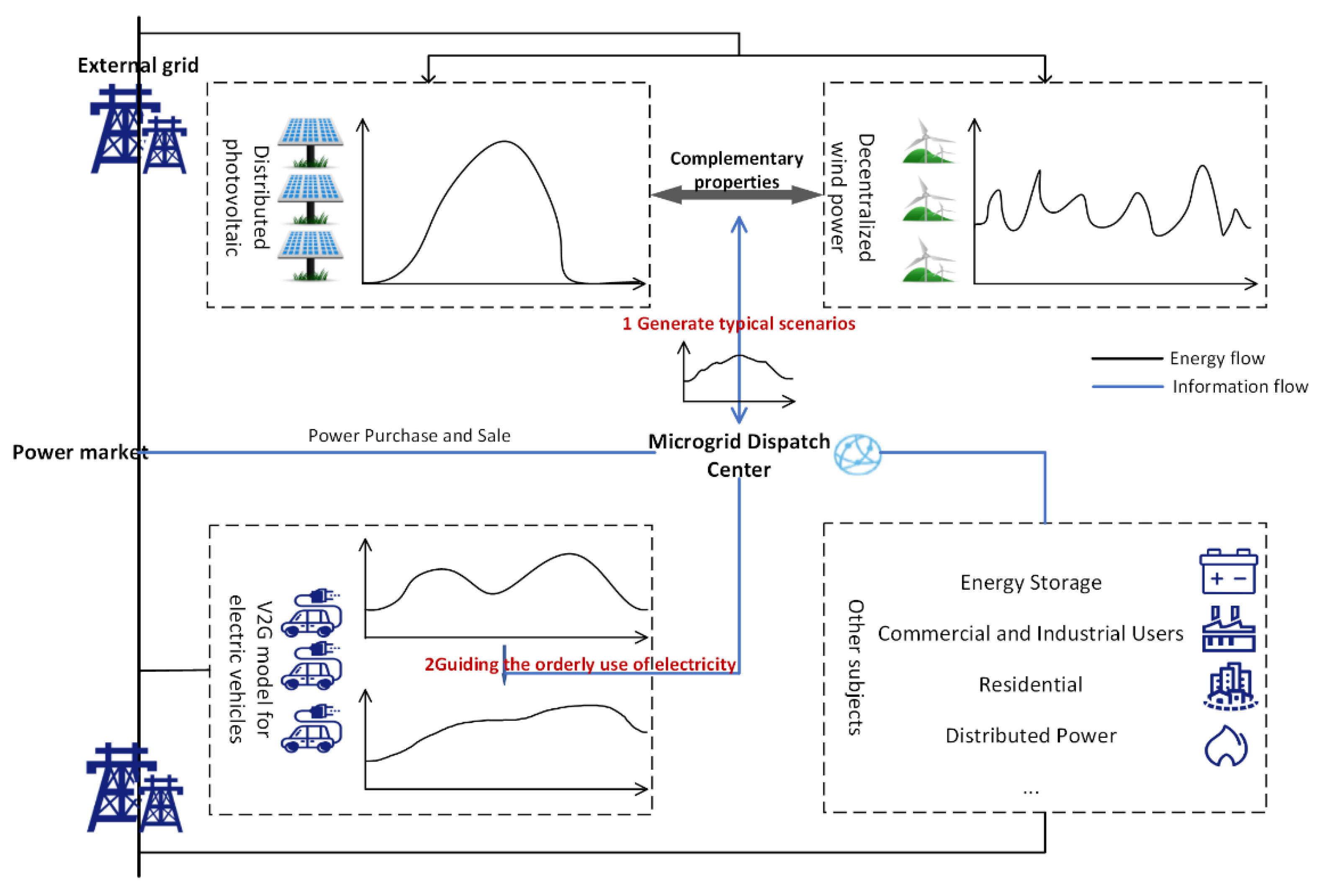
2. Microgrid Architecture Considering Wind–Solar Complementarity and V2G Technology

The microgrid studied in this paper primarily consists of the following components: Distributed Photovoltaics (DPV), Distributed Wind (DW), Electric Vehicles (EV), Storage Batteries (SB), Micro Turbines (MT), Distributed Generation (DG), commercial and industrial loads, residential loads, and a microgrid dispatch center. The structural diagram is illustrated in Figure 1. Among them, the microgrid scheduling center is responsible for aggregating the load situation of industrial and commercial users, residential users, and electric vehicles to the higher-level grid for the purchase and sale of electricity or to start demand response; distributed power supply, energy storage, electric vehicles, and distributed photovoltaic, decentralized wind power as the supply side of the production adjustment according to the scheduling instructions; industrial and commercial users, energy users and electric vehicles as the demand side of the energy according to the dispatch instructions for the start of the flexible response; the industrial and commercial users, energy users, and electric vehicles as the energy demand side responds flexibly according to the dispatch instructions.

This paper expands on traditional microgrid systems by emphasizing the complementary aspects of wind and solar energy. It highlights that strong sunlight occurs during the day along with higher wind speeds at night, while summer offers ample sunlight but weaker winds, and winter and spring experience increased winds with less sunlight. The spatiotemporal negative correlation between wind and solar energy suggests that treating them as a unified system can improve the stability of distributed renewable energy and create typical scenarios of combined wind–solar output, thus mitigating the uncertainty associated with renewable energy generation. Additionally, utilizing the V2G model, the microgrid scheduling center directs electric vehicles to consume electricity in a systematic manner, allowing for charging during peak photovoltaic generation and discharging when demand is highest. This strategy not only lowers charging expenses for vehicle owners but also helps manage load fluctuations within the microgrid.

3. Generation of Scenarios Considering the Uncertainty and Correlation of Wind and Solar Output

The output from wind and solar sources is greatly affected by factors like climate, weather conditions, and grid management, resulting in significant uncertainty and intensified load fluctuations within microgrids. To enhance the acceptance of renewable energy, reduce grid load variability, and achieve proper regulation of wind and solar outputs, it is crucial to analyze the uncertainties linked to wind and solar generation and investigate potential mitigation strategies. Moreover, examining the temporal complementarity between wind and photovoltaic (PV) generation can improve the economic efficiency and stability of microgrid operations, aiding in the integration of wind–solar power. Research indicates that copula functions are effective in modeling correlated variables, and models utilizing non-parametric kernel density estimation in conjunction with copula functions demonstrate high predictive accuracy [5,26]. Consequently, this study employs a non-parametric kernel density estimation approach to analyze historical data, enabling the derivation of kernel density functions for wind and solar outputs. Acknowledging the correlation between these outputs, the copula method is utilized to construct the joint probability distribution function.

When selecting the appropriate Copula function, it is observed that the Frank copula function does not impose restrictions on the direction or strength of correlation, whereas the Clayton copula and Gumbel copula functions are applicable only for positively correlated variables. Since wind and solar outputs generally exhibit a complementary negative correlation, the Frank copula function is chosen to characterize their relationship. Following this selection, sampling is conducted on the joint probability distribution function for each time frame, with corresponding wind power and PV outputs derived through inverse transformation based on the sampling outcomes and the joint probability density function. Finally, a backward reduction method is employed on the generated scenarios to produce representative typical scenarios.

3.1. Kernel Density Estimation

When examining the probability distribution model for wind speed and light intensity, researchers typically rely on two main approaches: the theoretical distribution model and kernel density estimation. The former is parameter-based, requiring the specification of a particular distribution in advance, which may overlook the inherent characteristics of the wind speed and light intensity curves. This can lead to significant discrepancies between the fitted parametric model and the actual data distribution [27]. In contrast, the nonparametric method does not necessitate prior knowledge of the sample model, allowing for the extraction of distribution characteristics directly from the provided data [28]. Therefore, this paper employs the nonparametric kernel density estimation technique to fit the actual data, yielding kernel density expressions for wind and light outputs after conducting goodness-of-fit and accuracy assessments.

When employing kernel density estimation (KDE), the approach involves measuring the distances between sample points within the neighborhood of x to assess how closely each sample point approaches x, thereby determining their influence on the estimated value $\widehat{f}\left(x\right)$. Assuming that the samples $X_1,X_2,\dots ,X_n$ drawn from X are independent and identically distributed, and that X follows an unknown density function $f\left(x\right)$, where $x\in \mathit{R}$, the objective is to estimate the probability density function value $\widehat{f}\left(x\right)$ at the point x:

$$\widehat{f}\left(x\right)={\displaystyle \frac{1}{nh}}{\displaystyle \sum }_{i=1}^{n}K\left({\displaystyle \frac{x-X_i}{h}}\right)$$

(1)

where n represents the sample size, h is the bandwidth, and K(·) denotes the kernel function.

The kernel density estimation method allows for non-parametric estimation of wind power and photovoltaic power data without the need for pre-established assumptions regarding the distribution of sample data, enabling the derivation of their respective probability density functions. The choice of kernel function significantly influences the results of the kernel density estimation, while the bandwidth h is another parameter that necessitates optimization. Furthermore, the integral mean squared error between the estimated and actual values is expressed as follows:

$$MISE\left(h\right)=\int E{\left[\widehat{f}\left(x\right)-f\left(x\right)\right]}^{2}dx$$

(2)

where E represents the weight matrix. By substituting $h_o$, obtained from minimizing Equation (2), into Equation (1), we can derive the overall kernel estimate.

3.2. Modeling of Wind and Light Output Correlation and Generation of Output Scenarios Based on Copula Theory

3.2.1. Copula Correlation Theory

(1) Copula function and correlation coefficient.

The expression of copula is:

$$F\left(x_1,x_2,\dots ,x_n\right)=C\left(F_{x_1}\left(x_1\right),F_{x_2}\left(x_2\right),\dots ,F_{x_n}\left(x_n\right)\right)$$

(3)

Copulas can be categorized into two primary families: Archimedean copulas and elliptical copulas. The three most prevalent Archimedean copula functions are the Gumbel, Clayton, and Frank copulas, while the primary elliptical copulas include the Gaussian and t-copulas.

The correlation coefficient serves to quantify the degree of linear association between variables, with common measures such as Kendall’s tau and Spearman’s rank correlation coefficient.

(2) Optimal Selection of Copula Functions.

Given the diversity of copula functions, directly selecting the most suitable one is impractical; therefore, goodness-of-fit tests are essential for determining the best option. Typical methods for this include graphical analysis of copulas, correlation coefficient evaluation, and Euclidean distance analysis.

a. In graphical analysis, the probability density function (PDF) graphs of different copula functions are compared with the PDF of the observed data. The copula function whose graph is closest to the sample data is deemed ideal.

b. The correlation coefficient evaluation method measures goodness-of-fit using Kendall’s tau and Spearman’s rank correlation coefficients. By comparing the rank correlation coefficients from various copula functions with those from the sample data, a closer match indicates a better fit, thus identifying the optimal copula function.

Let U and V represent the outputs of a correlated wind farm and photovoltaic power station, respectively. ($u_1,v_1$) and ($u_2,v_2$) are any two observed output sample values of (U, V), which are independent of each other. If ($u_1,v_1$)$\bullet$($u_2,v_2$) > 0, then ($u_1,v_1$) and ($u_2,v_2$) are said to exhibit consistency; if ($u_1,v_1$)$\bullet$($u_2,v_2$) < 0, then ($u_1,v_1$) and ($u_2,v_2$) are considered inconsistent.

The formulas for calculating Kendall’s rank correlation coefficient ${\rho }_k$ and Spearman’s rank correlation coefficient ${\rho }_s$ are as follows:

$${\rho }_k={\displaystyle \frac{2\left(a-b\right)}{N\left(N-1\right)}}$$

(4)

$${\rho }_s={\displaystyle \frac{{{\displaystyle \sum }}_{i=1}^N\left(c_i-\overline{c}\right)\left(d_i-\overline{d}\right)}{\sqrt{{{\displaystyle \sum }}_{i=1}^N{\left(c_i-\overline{c}\right)}^2}\sqrt{{{\displaystyle \sum }}_{i=1}^N{\left(d_i-\overline{d}\right)}^2}}}$$

(5)

where a denotes the number of sample pairs in $(U, V)$ that exhibit consistency, while $b$ represents the number of sample pairs that show inconsistency. $N$ is the total number of sampling points, which in this study is taken to be 24, corresponding to a sampling interval of 1 h. Additionally, $c_i$ refers to the rank of $u_i$ in the sequence $(u_1,u_2,\dots ,u_N)$, and $d_i$ refers to the rank of $v_i$ in the sequence $(v_1,v_2,\dots ,v_N)$. The mean ranks are defined as $\overline{c}={\sum }_{i=1}^N{\displaystyle \frac{c_i}{N}}$ and $\overline{d}={\sum }_{i=1}^N{\displaystyle \frac{d_i}{N}}$.

c. The Euclidean distance discriminant method compares the Euclidean distances between each copula function and the empirical copula function derived from the sample data. A smaller Euclidean distance indicates a better goodness-of-fit for the copula function. Let ($x_i$, $y_i$) for (i = 1, 2, $\dots$, n) represent the sample of the two-dimensional variables $(X,Y)$. The empirical cumulative distribution functions for the two-dimensional variables (X, Y) are denoted as $F_n\left(x_i\right)$ and $F_n\left(y_i\right)$, respectively. The formula for calculating the empirical copula function of the sample is given by:

$$C_n\left(u,v\right)={\displaystyle \frac{1}{n}}{\displaystyle \sum }_{i=1}^n{I}_{\left[F_n\left(x_i\right)\le u\right]}{I}_{\left[G_n\left(y_i\right)\le v\right]}$$

(6)

where $I_{[\bullet ]}$ represents the indicator function. Specifically, when $F_n\left(x_i\right)\le u$, we have $I_{\left[F_n\left(x_i\right)\le u\right]}$ = 1; otherwise, $I_{\left[F_n\left(x_i\right)\le u\right]}$ = 0. Similarly, the function $I_{\left[G_n\left(y_i\right)\le v\right]}$ is defined in an analogous manner.

The optimal Copula function is selected using the squared Euclidean distance. The definition of the squared Euclidean distance is:

$$d^2={\displaystyle \sum }_{i=1}^n{\left|C_n\left(u_i,v_i\right)-C_e\left(u_i,v_i\right)\right|}^2$$

(7)

where $u_i=F_n\left(x_i\right)$ and $v_i=G_n\left(y_i\right)$, where $C_e\left(\bullet \right)$ represents the empirical copula function.

The magnitude of the selected squared Euclidean distance reflects the degree of proximity between various copula function models and the empirical copula function. A smaller value of $d^2$ indicates better fitting performance of the function.

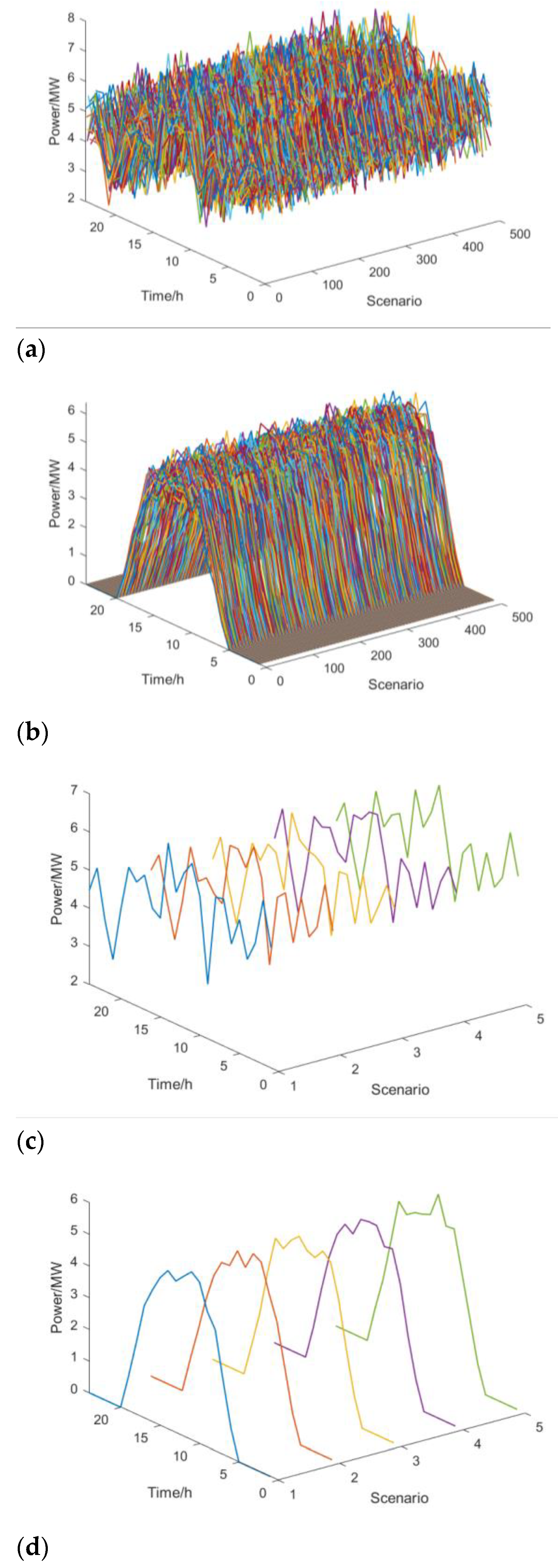
3.2.2. Generation of Wind–Solar Scenarios and Complementarity Characteristics

Static Scenario Generation and Reduction of Wind–Solar Output Using Monte Carlo Simulation:

(1)

Generate random numbers $a_1,a_2,\dots ,a_n$ within the interval [0,1].

(2)

Assign the marginal distribution function value of the first random variable as $u_1=a_1$. Next, compute the marginal distribution function value of the second random variable $u_2$ by applying the copula function chosen in Section 3.2.1, which involves solving Equation (8).

After determining the optimal copula function, large-scale samples can be produced by sampling from the selected copula using the following steps:

(1)

Generate random values in the range [0,1].

(2)

With the marginal distribution function value of the first random variable established, calculate the value of the second random variable’s marginal distribution function based on the copula function identified in Section 3.2.1, effectively resolving Equation (8).

$${\displaystyle \frac{\partial C\left(u_1,u_2,\cdots ,u_n\right)}{\partial u_1}}=a_2$$

(8)

(3)

The marginal distribution function value of the n-th random variable should be regarded as the solution to Equation (9).

$${\displaystyle \frac{\frac{{\partial }^{n-1}C\left(u_1,u_2,\cdots ,u_n\right)}{\partial u_1\partial u_2\cdots \partial u_{n-1}}}{\frac{{\partial }^{n-1}C\left(u_1,u_2,\cdots ,u_{n-1},1\right)}{\partial u_1\partial u_2\cdots \partial u_{n-1}}}}=a_n$$

(9)

(4)

By repeating Steps (1), (2), and (3) a total of k times, k sets of marginal distribution function values for n random variables can be obtained.

(5)

By performing the inverse function operation, the results can be transformed into a joint distribution function scenario, where the index j ranges from 1 to T, with T representing the total number of days.

In the analysis of wind and solar power generation, the inverse function operations in Step (5) must first compute the marginal distribution functions for both sources based on the copula joint probability density, followed by their respective inverse function calculations. This methodology effectively accounts for the correlation between wind and solar outputs. The large volume of data generated through scenario creation exhibits high similarity among scenes. To effectively merge similar scenarios, a backward reduction (BR) method is employed for scenario reduction. The scenario reduction process based on the backward elimination method is illustrated in Figure 2.

3.2.3. Indicators of Wind–Solar Complementarity Characteristics

The coefficient of variation (CV) is chosen to represent the complementarity between wind power and photovoltaic output. The definition of CV is as follows:

$$CV={\displaystyle \frac{\sqrt{\frac{1}{N}{{\displaystyle \sum }}_{t=1}^N{(P_t^{WT}+P_t^{PV}-\overline{P})}^2}}{\overline{P}}}$$

(10)

$$\overline{P}={\displaystyle \frac{1}{N}}{\displaystyle \sum }_{t=1}^N\left(P_t^{WT}+P_t^{PV}\right)$$

(11)

where $P_t^{WT}$ and $P_t^{PV}$ represent the wind power output and photovoltaic output at the t-th sampling point, respectively, while $\overline{P}$ denotes the average power of both sources.

According to Equation (13), a lower CV indicates that the combined output power of wind and photovoltaic sources is more stable, thus demonstrating superior complementary characteristics. To ensure that the generated wind–solar scenarios exhibit stable output and favorable complementary properties, the CV must be maintained below the system-defined reference values ${\epsilon }_1$ and ${\epsilon }_2$, such that CV $\le {\epsilon }_1$ and CV $\le {\epsilon }_2$. Here, ${\epsilon }_1$ and ${\epsilon }_2$ correspond to the CV values for the scenarios where only wind power and only photovoltaic power are utilized, respectively:

$$\left\{\begin{array}{c}{\epsilon }_1={\displaystyle \frac{{{\displaystyle \sum }}_{i=1}^T\frac{\sqrt{\frac{1}{N_i}{{\displaystyle \sum }}_{t=1}^{N_i}\left(P_{i,t}^{WT}-\overline{P_i^{WT}}\right)}}{\overline{P_i^{WT}}}}{T}}\\ {\epsilon }_2={\displaystyle \frac{{{\displaystyle \sum }}_{i=1}^T\frac{\sqrt{\frac{1}{N_i}{{\displaystyle \sum }}_{t=1}^{N_i}\left(P_{i,t}^{PV}-\overline{P_i^{PV}}\right)}}{\overline{P_i^{PV}}}}{T}}\end{array}\right.$$

(12)

$$\left\{\begin{array}{c}\overline{P_i^{WT}}={\displaystyle \frac{1}{N_i}}{\displaystyle {\displaystyle \sum }_{t=1}^{N_i}}{P}_{i,t}^{WT}\\ \overline{P_i^{PV}}={\displaystyle \frac{1}{N_i}}{\displaystyle {\displaystyle \sum }_{t=1}^{N_i}}{P}_{i,t}^{PV}\end{array}\right.$$

(13)

where $P_{i,t}^{WT}$ denotes the wind power output at the t-th sampling instance on the i-th day; $P_{i,t}^{PV}$ signifies the photovoltaic power output at the t-th sampling instance on the i-th day; $\overline{P_i^{WT}}$ represents the average wind power output for the i-th day; $\overline{P_i^{PV}}$ refers to the average photovoltaic power output for the i-th day; and $N_i$ indicates the total number of sampling instances on the i-th day.

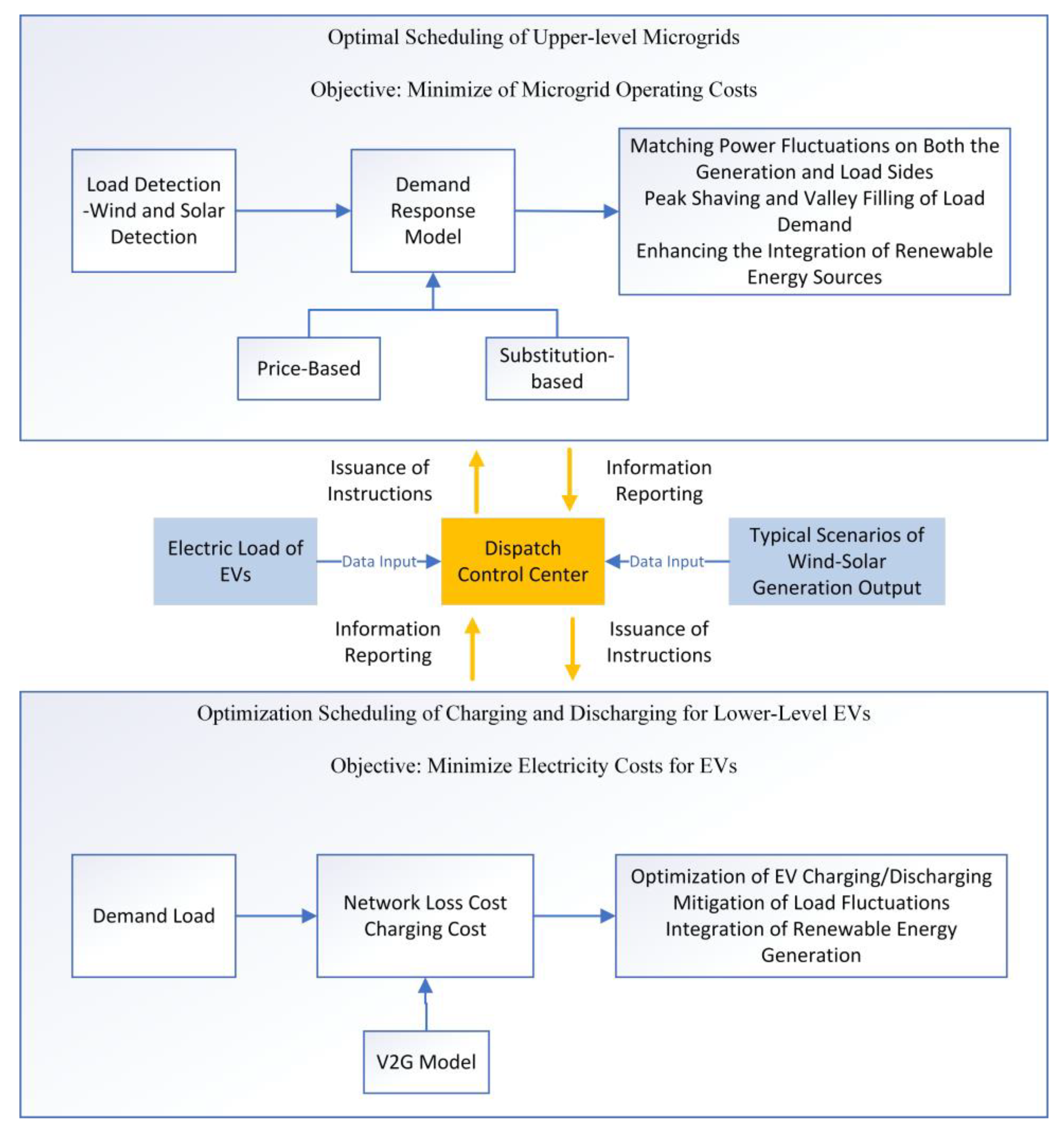
4. Hierarchical Optimization Scheduling Model for Microgrid

4.1. Hierarchical Optimization Scheduling Strategy

This study proposes an optimization scheduling model for microgrids that integrates EVs, based on typical scenarios of wind and solar power generation. A hierarchical optimization scheduling method that incorporates demand response has been developed for this model, as shown in Figure 3.

The process begins by gathering data on standard wind and solar generation patterns and the electricity consumption of EVs. The upper-level model then applies a load demand response framework to optimize the performance of various devices, with the goal of minimizing system load fluctuations and maximizing renewable energy usage. The outcomes from the upper-level optimized EV load scheduling serve as a reference trajectory for the lower-level EV scheduling. Finally, real-time optimization techniques are employed to oversee the charging and discharging processes of EVs, enhancing the capability for renewable energy absorption while reducing the overall charging load of EVs.

4.2. Demand Response Program Model

4.2.1. Price-Based Demand Response

Electric loads that participate in price-based demand response are generally categorized into curtailable loads (CL) and shiftable loads (SL).

(1) Modeling the Characteristics of CL

CL adjusts its load in response to changes in electricity prices. It evaluates price variations before and after engaging in demand response to decide whether to decrease its load. To effectively characterize this response, a price elasticity matrix, E(t,j), is created. This matrix defines the elasticity coefficient of load at time t concerning the electricity price at time j, represented by $e_{t,j}$—the element found at the intersection of the t-th row and the j-th column in the matrix. The mathematical formulation is as follows:

$$e_{i,j}={\displaystyle \frac{\frac{\Delta L_{E,t}}{L_{E0,t}}}{\frac{\Delta {\pi }_j}{{\pi }_{0,j}}}}$$

(14)

where $∆L_{E,t}$ and $L_{E0,t}$ indicate the change in load at time t following the demand response and the initial load, respectively. Moreover, $∆{\pi }_j$ and ${\pi }_{0,j}$ signify the price change at time j following the demand response and the initial price, respectively.

The formula for the change in CL at time t after executing the demand response is:

$$\Delta L_{ECL,t}=L_{ECL0,t}\left[{\displaystyle \sum }_{j=1}^{24}{E}_{CL}\left(t,j\right){\displaystyle \frac{{\pi }_j-{\pi }_{0,j}}{{\pi }_{0,j}}}\right]$$

(15)

where $E_{CL}\left(t,j\right)$ represents the price elasticity matrix of CL; $L_{ECL0,t}$ denotes the initial reducible load at time t; and ${\pi }_j$ signifies the electricity price at time j.

(2) Modeling Transferable Load Characteristics

Without affecting normal operations, SL can flexibly shift over time in response to changes in electricity price signals. Similarly, the price elasticity matrix describes the demand response characteristics. The mathematical expression for the change in SL at time t after demand response is given by:

$$\Delta L_{ESL,t}=L_{ESL0,t}\left[{\displaystyle \sum }_{j=1}^{24}{E}_{SL}\left(t,j\right){\displaystyle \frac{{\pi }_j-{\pi }_{0,j}}{{\pi }_{0,j}}}\right]$$

(16)

where $L_{ESL0,t}$ represents the initial transferable load amount at time t.

4.2.2. Replaceable Demand Response

Replaceable Load (RL) refers to the ability to autonomously choose to utilize electrical or thermal energy based on fluctuations in electricity prices to meet its thermal load demands. The mathematical expression for the change in replaceable electrical load at time t following demand response is as follows:

$${\Delta L}_{ERL,t}=-{\epsilon }_{E,H}{\Delta L}_{HRL,t}$$

(17)

$${\epsilon }_{E,H}={\displaystyle \frac{v_E{\phi }_E}{v_H{\phi }_H}}$$

(18)

where $∆L_{ERL,t}$ denotes the change in replaceable thermal load at time t; ${\epsilon }_{E,H}$ represents the electrical and thermal substitution coefficients; ${\phi }_E$ and ${\phi }_H$ are the utilization rates of electricity and thermal energy, respectively; and $v_E$ and $v_H$ indicate the unit calorific values of electricity and thermal energy, respectively.

4.3. Upper-Level Optimization Model

4.3.1. Objective Function

The objective of the upper-level microgrid is to minimize the total operating and environmental protection costs $C_{total}$. This primarily includes the microgrid operational cost $C_1$, the environmental protection cost $C_2$, and the penalties for wind and solar curtailment $C_3$. The specific objective function is expressed as:

$$min{C}_{total}=C_1+C_2+C_3$$

(19)

(1) Microgrid Operational Cost

The operational cost of the microgrid encompasses fuel costs, the operational and maintenance costs of the microgrid, interaction costs with the main grid, depreciation costs of electric vehicle batteries, and demand response costs of the microgrid. Hence, the operational cost for this scheduling model is defined as follows:

$$C_1={\displaystyle \sum }_{i=1}^N{\displaystyle \sum }_{t=1}^T\left[F_i\left(P_i\left(t\right)\right)+O{M}_i\left(P_i\left(t\right)\right)\right]+C_{GRID}+C_{BAT}+C_{DR}+C_{ESS}+C_{PV}+C_{WT}$$

(20)

where $C_1$ denotes the operational cost of the microgrid; i represents the index of DGs; N is the total number of DGs in the microgrid; T refers to the total number of time periods within the scheduling cycle; t is the specific time period; $P_i$ indicates the actual output power of the i-th DG; $F_i\left(P_i\right)$ represents the fuel cost associated with the i-th DG; ${OM}_i\left(P_i\right)$ signifies the operation and maintenance cost of the i-th DG; $C_{GRID}$ refers to the interaction cost between the microgrid and the main grid; $C_{BAT}$ is the depreciation cost of electric vehicle batteries; $C_{DR}$ indicates the demand response cost for microgrid loads; $C_{ESS}$ refers to the operational cost of energy storage systems; and $C_{PV}$ and $C_{WT}$ denote the operation and maintenance costs for photovoltaic and wind turbine systems, respectively. The details are as follows:

$$O{M}_i\left(P_i\left(t\right)\right)=K_{O{M}_i}{P}_i\left(t\right)$$

(21)

$$C_{GRID}={\displaystyle \sum }_{t=1}^T\left|P_{GRID}\left(t\right)\right|S_t$$

(22)

where $K_{{OM}_i}$ denotes the operation and maintenance coefficient for the i-th distributed generator DG; $P_{GRID}$ indicates the transmission power between the microgrid and the main grid (with a positive value representing power flowing from the main grid to the microgrid and a negative value indicating power being supplied to the main grid from the microgrid). $S_t$ refers to the electricity price during period t; a positive value implies that the microgrid is purchasing electricity, while a negative value suggests that the microgrid is selling electricity.

As the charging capacity increases with each cycle, the overall number of charging cycles for the battery decreases, which complicates the total cycle count calculation. To simplify this process, this study assumes that the total charge and discharge capacity of the battery remains consistent throughout its lifecycle. Therefore, the depreciation cost associated with the electric vehicle battery can be formulated as follows:

$$C_{BAT}={\displaystyle \sum }_{j=1}^n\left({\displaystyle \frac{C_{REP}}{E_{PUT}}}\underset{t_{j1}}{\overset{t_{j2}}{{\displaystyle \int }}}\left|P_j^{EV}\left(t\right)dt\right|\right)$$

(23)

where n denotes the total number of EVs, $C_{REP}$ refers to the replacement cost of the EV battery, and $E_{PUT}$ represents the total charge and discharge capacity of the battery over its lifespan. $t_{j1}$ and $t_{j2}$ indicate the connection start and end times for the j-th EV to the microgrid, while $P_j^{EV}\left(t\right)$ denotes the power associated with the j-th EV’s charging and discharging during period t (with positive values reflecting discharge and negative values indicating charging).

The microgrid has the capability to adaptively modify the demand response load schedule; however, adjustments to the power consumption plan will likely impact user comfort. Thus, it is essential for the microgrid to offer suitable compensation. The necessary scheduling cost $C_{DR}$ can be formulated as follows:

$$C_{DR}=K_{DR}\left|P_{DR}\left(t\right)-P_{DR}^{*}\left(t\right)\right|\Delta t$$

(24)

where $K_{DR}$ signifies the unit scheduling cost for demand response loads; $P_{DR}\left(t\right)$ indicates the actual scheduled power of the demand response load at time t; and $P_{DR}^{\mathrm{*}}\left(t\right)$ represents the anticipated power consumption of the demand response load during the same time period.

The operational expenses of energy storage mainly encompass the initial investment and maintenance costs. The average charging and discharging cost $C_{ESS}$ during time t within the investment recovery timeframe can be articulated as follows:

$$C_{ESs}\left(t\right)=K_s\left[{\displaystyle \frac{P_s^{dis}\left(t\right)}{\eta }}+P_s^{cha}\left(t\right)\eta \right]\Delta t$$

(25)

where $K_s$ corresponds to the equivalent costs for charging and discharging; $P_s^{cha}\left(t\right)$ and $P_s^{dis}\left(t\right)$ represent the charging and discharging power on the AC side of the energy storage inverter during time t, respectively; and $\eta$ indicates the energy storage unit’s charge and discharge efficiency.

Regular maintenance is necessary for distributed photovoltaic and wind turbine systems, and the associated maintenance costs can be expressed as follows:

$$C_{PV}={\displaystyle \sum }_{t=1}^T({\alpha }_{PV}{P}_{PV}\left(t\right))$$

(26)

$$C_{WT}={\displaystyle \sum }_{t=1}^T({\alpha }_{WT}{P}_{WT}\left(t\right))$$

(27)

where ${\alpha }_{PV}$ and ${\alpha }_{WT}$ indicate the operational maintenance cost coefficients for photovoltaic and wind power systems, respectively. Meanwhile, $P_{PV}\left(t\right)$ and $P_{WT}\left(t\right)$ represent the output power generated by the photovoltaic and wind turbine systems at time t.

(2) Environmental Protection Costs of Microgrids

The operation of distributed microgrid power generation, as well as that of the main grid, can lead to environmental pollution issues. The environmental protection costs are specifically defined as follows:

$$C_2={\displaystyle \sum }_{i=1}^N{\displaystyle \sum }_h^H\left(C_h{u}_{ih}\right)P_i+{\displaystyle \sum }_h^H\left(C_h{u}_{gridh}\right)P_{grid}$$

(28)

where h signifies the level of pollutant emissions; H represents the total emissions, including ${CO}_2$, ${SO}_2$, and ${NO}_X$; $u_{ih}$ and $u_{gridh}$ are the emission coefficients for DG and the main grid, respectively; $C_h$ denotes the treatment cost associated with emissions of the h-th pollutant; and $P_{grid}$ refers to the power output from the main grid.

(3) Penalty costs for curtailed wind and solar energy in microgrids:

$$C_3={\lambda }_{WT}{\displaystyle \sum }_{t=1}^T{P}_{qWT}\left(t\right)+{\lambda }_{PV}{\displaystyle \sum }_{t=1}^T{P}_{qPV}\left(t\right)$$

(29)

where $P_{qWT}\left(t\right)$ and $P_{qPV}\left(t\right)$ indicate the curtailed wind and solar energy during time period t, respectively. ${\lambda }_{WT}$ and ${\lambda }_{PV}$ represent the penalty costs per unit for curtailed wind and solar power, respectively.

4.3.2. Constraints

The proposed optimization scheduling model encompasses several constraints in addition to the balance of power supply and demand, limits on generation capacity, and ramp rate restrictions for DG. It also includes transmission capacity constraints between the microgrid and the main grid, along with energy storage capacity and operational limitations, thereby improving the model’s overall comprehensiveness. The specific constraints are outlined as follows:

(1) Power Supply-Demand Balance Constraint

$${\displaystyle \sum }_{i=1}^N{P}_i+P_{GRID}+P_{EV}+P_{PV}+P_{WT}+(P_s^{dis}\left(t\right)+P_s^{cha}\left(t\right))\eta =P_{LOAD}+P_{DR}\left(t\right)$$

(30)

where $P_i$ represents the current output of the DG; $P_{GRID}$ refers to the power transmitted between the microgrid and the main grid; $P_{EV}$ indicates the net output from electric vehicles; $P_{PV}$ denotes the actual power generated by PV systems; $P_{WT}$ represents the actual power produced by WT; and $P_{LOAD}$ signifies the overall load demand.

(2) Generation Capacity Constraints

The actual output from each DG is required to stay within its defined upper and lower output limits, which can be expressed as:

$$P_i^{min}\le P_i\le P_i^{max}$$

(31)

where $P_i^{max}$ and $P_i^{min}$ indicate the maximum and minimum output power limits for the i-th distributed DG, respectively.

(3) Ramp Rate Limitation of DG

The ramp rate refers to the variation in output power of the DG over time, which reflects its operational performance. The limits for the ramp rate of the DG can be articulated as follows:

$$\left|P_i\left(t\right)-P_i\left(t-1\right)\right|\le r_i$$

(32)

where $P_i\left(t\right)$ and $P_i(t-1)$ represent the output power of the DG at time periods t and t − 1, respectively, while $r_i$ denotes the upper limit of the ramp rate for the DG during this period.

(4) Limitations on Transmission Capacity

The connection between the microgrid and the main grid requires the establishment of a transmission agreement, ensuring that the power transmitted between the microgrid and the main grid does not exceed specified limits:

$$P_{buy}^{min}\le P_{DRID}\left(t\right)\le P_{buy}^{max}$$

(33)

$$P_{sell}^{min}\le P_{DRID}\left(t\right)\le P_{sell}^{max}$$

(34)

where $P_{DRID}$ denotes the power exchanged between the microgrid and the main grid, with $P_{buy}^{min}$ and $P_{buy}^{max}$ representing the minimum and maximum transmission power limits for purchasing electricity from the main grid. Likewise, $P_{sell}^{min}$ and $P_{sell}^{max}$ establish the minimum and maximum transmission power limits for selling electricity to the main grid.

(5) Operational Constraints of Energy Storage Units:

$$0\le P_s^{dis}\left(t\right)\le U_s\left(t\right)P_s^{max}$$

(35)

$$0\le P_s^{cha}\left(t\right)\le \left[1-U_s\left(t\right)\right]P_s^{max}$$

(36)

$$\eta {\displaystyle \sum }_{t=1}^{N_T}\left[P_s^{cha}\left(t\right)\Delta t\right]-{\displaystyle \frac{1}{\eta }}{\displaystyle \sum }_{t=1}^{N_T}\left[P_s^{dis}\left(t\right)\Delta t\right]=0$$

(37)

$$E_s^{min}\le E_s\left(0\right)+\eta {\displaystyle \sum }_{t^{\prime }=1}^t\left[P_s^{cha}\left(t^{\prime }\right)\Delta t\right]-{\displaystyle \frac{1}{\eta }}{\displaystyle \sum }_{t^{\prime }=1}^t\left[P_s^{dis}\left(t^{\prime }\right)\Delta t\right]\le E_s^{max}$$

(38)

where (35) and (36) define the power limits for the charging and discharging processes of the energy storage system, respectively. $P_s^{max}$ indicates the maximum charge and discharge power, primarily restricted by the capacity of the grid-connected inverter. $U_s\left(t\right)$ represents the state of charge of the storage unit, with a value of 1 signifying discharge and 0 indicating charge. Equation (37) guarantees that the energy storage capacity at the beginning and end of the scheduling period remains unchanged, thus enabling cyclic operation. $N_T$ refers to the scheduling period, which is set to 24 h. Equation (38) outlines the constraints on remaining capacity for each time period, where $E_s\left(0\right)$ signifies the initial capacity at the start of scheduling, while $E_s^{max}$ and $E_s^{min}$ denote the permissible maximum and minimum remaining capacities, respectively. These constraints aim to prevent both overcharging and deep discharging of the energy storage system, thereby enhancing its lifespan.

(6) Demand Response Load Constraints

In the framework of a microgrid featuring shiftable loads, the electricity consumption patterns during demand response service provision can be illustrated by the following constraints:

$${\displaystyle \sum }_{t=1}^{N_T}{P}_{DR}\left(t\right)\Delta t=D_{DR}$$

(39)

$$D_{DR}^{min}\left(t\right)\le P_{DR}\left(t\right)\Delta t\le D_{DR}^{max}\left(t\right)$$

(40)

where $P_{DR}\left(t\right)$ refers to the actual scheduled power for demand response loads within the microgrid at time t; $D_{DR}$ signifies the total electricity demand of these loads throughout the scheduling period; $D_{DR}^{max}\left(t\right)$ and $D_{DR}^{min}\left(t\right)$ represent the maximum and minimum electricity demands of demand response loads at time t, both of which are linked to user comfort needs.

4.4. Lower-Level Optimization Model

4.4.1. Objective Function

The objective of this phase is to minimize the total energy cost of EVs. Within a scheduling period, the total cost associated with the charging cost $C_{EV,1}$ and line loss cost $C_{EV,2}$ represents the overall cost for EVs to complete their charging tasks. The specific objective function is given by:

$$min{C}_{EV}=C_{EV,1}+C_{EV,2}$$

(41)

(1) Charging Cost

The charging cost for EVs is defined as the total cost of electricity acquired for both charging and discharging when connected to the power grid. The overall load for charging and discharging of EVs linked to the grid can be denoted as $L_{EV,t}$, and can be mathematically represented as:

$$L_{EV,t}={\displaystyle \sum }_{i=1}^N{P}_{EV,i,t}$$

(42)

Let the baseline load of the EV be denoted as $L_{base,t}$. The total load of the EV scheduled over the time period t, $L_{z,t}$, can be expressed as:

$$L_{z,t}=L_{base,t}+L_{EV,t}$$

(43)

Assuming that the real-time electricity price for EV charging varies linearly with the total load of the EV during each time period, the mathematical representation can be expressed as:

$$g\left(L_{z,t}\right)=k_0+k_1{L}_{z,t}$$

(44)

Thus, the charging cost for the EV can be expressed as:

$$C_{ch,t}={{\displaystyle \int }}_{L_{base,t}}^{L_{z,t}}g\left(L_{z,t}\right)d{L}_{z,t}$$

(45)

Thus, the total charging cost for the EV is:

$$C_{EV,1}={\displaystyle \sum }_{t=1}^T{C}_{ch,t}$$

(46)

(2) Network Loss Cost

When an EV transfers stored energy back to the grid, it may result in problems like frequency and voltage instability. As a result, V2G technology can contribute to network losses in real grid operations. These losses are incorporated as an economic cost within the EV’s charging and discharging expenses. For a grid with m branches, the active power loss in these branches during a specific time period t can be represented as:

$$P_{loss,t,m}=R_m{\left(\left|V_{ml}-V_{mr}\right|\left|Y_m\right|\right)}^2$$

(47)

where $R_m$, $V_{ml}$, $V_{mr}$, and $Y_m$ represent the resistance of the branch, the voltages at the two terminal nodes, and the admittance, respectively.

The network loss cost during the time period t can be expressed as:

$$P_{loss,t}={\displaystyle \sum }_{m=1}^M{P}_{loss,t,m}$$

(48)

Therefore, the total network loss cost can be expressed as:

$$C_{EV,2}={\displaystyle \sum }_{t=1}^T{k}_2{P}_{loss,t}$$

(49)

where $k_2$ represents the conversion coefficient for network loss costs.

4.4.2. Constraints

The real-time scheduling duration for charging and discharging an EV spans 24 h, segmented into T = 48 time slots, each lasting τ = 30 min. When an EV is connected to a smart charging station, the station sends pertinent information about the connected vehicle through the charging data line at the start of each optimized scheduling period to refresh the initial data in the scheduling center. The available scheduling time $T_{opt,i}$ for the EV can be calculated based on the entry time $t_{in,i}$ and the target departure time $t_{off,i}$ as follows:

$$T_{opt,i}=t_{off,i}-t_{in,i}$$

(50)

Let the matrix $P_{EV}$ represent the charging and discharging schedule of the EV over a single scheduling period:

$$P_{EV}=\left[\begin{array}{ccc}{P}_{EV,1,1}& \dots & P_{EV,1,T}\\ ⋮& \ddots & ⋮\\ P_{EV,N,1}& \dots & P_{EV,N,T}\end{array}\right]$$

(51)

where $P_{EV,i,t}>0$ and $P_{EV,i,t}<0$ denote the charging and discharging power of electric vehicle i during time period t, respectively.

(1) Charging and Discharging Power Constraints:

$$P_{EV,Dch}<P_{EV,i,t}<P_{EV,Ch},\forall i\in N_{V2G},\forall t\in T$$

(52)

where $P_{EV,Ch}$ and $P_{EV,Dch}$ represent the maximum charging and discharging power of the EV, respectively. $N_{V2G}$ denotes the total number of N EVs connected to the grid that support the V2G mode.

(2) Battery State of Charge Constraint

Let $E_{in,i}$ represent the initial state of charge of the electric vehicle (EV) when it is connected to the grid, and $E_{off,i}$ denote the off-grid target state of charge established by the user. Consequently, the battery state of charge at the moment of disconnection must fulfill the following condition:

$$E_{in,i}+{\displaystyle \sum }_{t=t_{in,i}}^{t_{off,i}}\tau P_{EV,i,t}\ge E_{off,i},\forall i\in N$$

(53)

Additionally, at any moment during the dispatchable period, the battery state of charge of the EV must satisfy the following constraint:

$$0\le E_{in,i}+{\displaystyle \sum }_{t=t_{in,i}}^{t_{q,i}}\tau P_{EV,i,t}\le E_{CAP,i},\forall i\in N,\forall t_{q,i}\in \left[t_{in,i},t_{off,i}\right]$$

(54)

where $E_{CAP,i}$ represents the maximum capacity of the EV battery.

4.5. Bi-Level Optimization Scheduling Model Solution

4.5.1. Upper-Level Solution

For the optimization scheduling problem of the upper-level microgrid, we first analyze the demand response model to determine the load after demand response. Subsequently, under the constraints of energy power balance and energy conversion for each device, the established model is transformed into a mixed-integer linear model using piecewise linearization. This model is then solved using the Gurobi solver via the Yalmip toolbox in MATLAB.

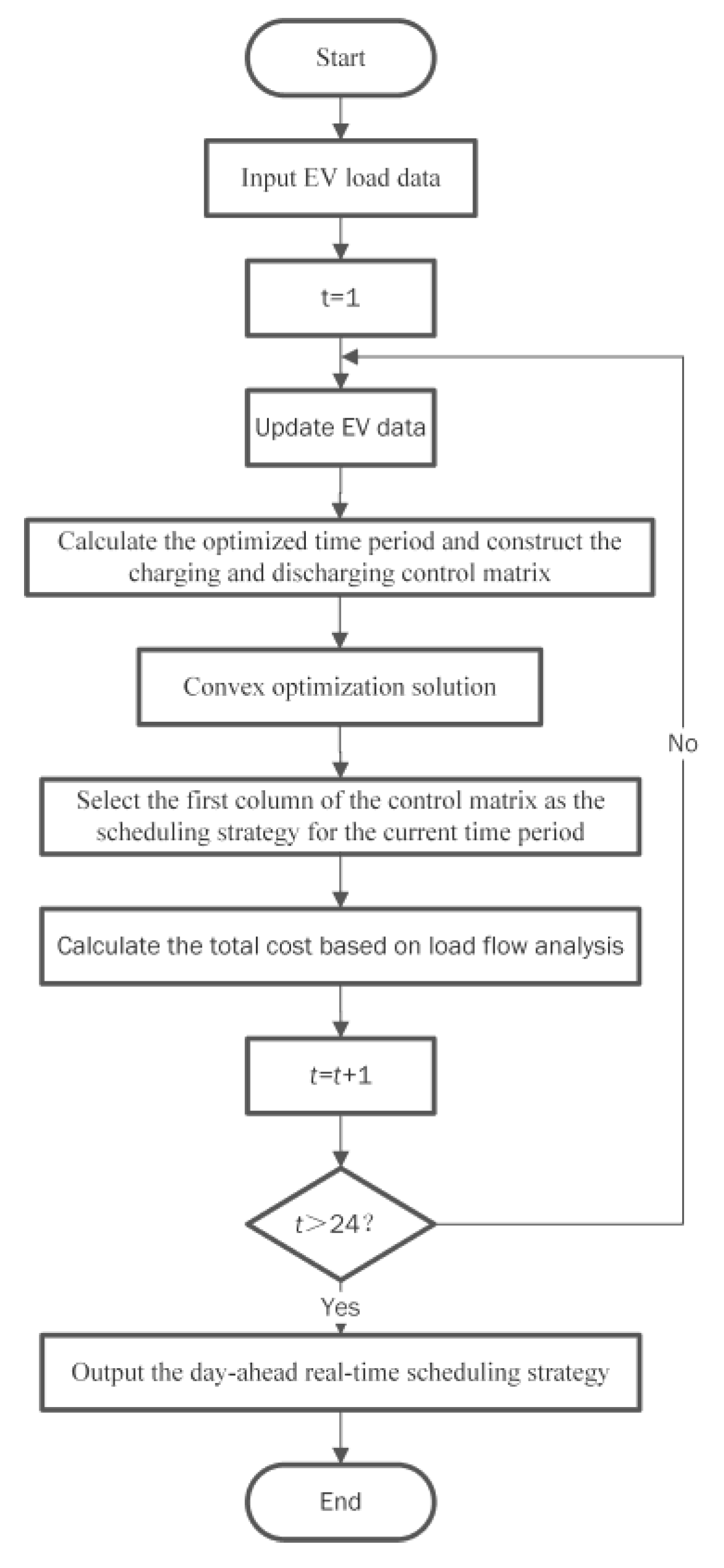
4.5.2. Lower-Level Solution

Within the time period t, the total number of dispatchable EVs is denoted as N’, which can be categorized into two types: the first type includes EVs that have been connected to the charging station for a certain duration, satisfying the condition $t_{in,i}<t<t_{off,i}$; the second type consists of EVs that are connected to the charging station during this time period, satisfying $t_{in,i}=t$. For these EVs, their remaining dispatchable time is defined as $H_{left,i}=t_{off,i}-t$.

As illustrated in Figure 4, to enable the real-time charging and discharging strategy to more effectively align the EV energy consumption load with the variations in upper-level EV demand response loads during the current time period, the size of the optimization time window must dynamically adapt according to changes in the load curve. By calculating the remaining dispatchable time for the currently available EVs and taking the maximum value, the optimal range of the time period t can be determined as $W_t$.

$$W_t=max\left\{\cup H_{left,i},i\in N^{\prime }\right\}$$

(55)

The scheduling process is illustrated in Figure 5. Firstly, before the start of the scheduling cycle, the scheduling center updates the baseline load data for EVs and arranges and numbers the EVs based on their connection time to prepare for the dispatch of the lower-level model. Subsequently, this load data is used in the upper-level demand response load optimization. At the beginning of each real-time scheduling period, the data for dispatchable EVs, denoted as $N’$, is updated. The optimization range $W_t$ for the current scheduling period is determined based on the remaining dispatchable time of the EVs. Using N’ and $W_t$, the EV charging and discharging scheduling control matrix $X^{″}$ is constructed, and the first column of this matrix is taken as the EV scheduling strategy for the current period. Finally, the optimized load is updated along with the real-time scheduling load of the EVs into the power grid to calculate the total electricity cost for the current period.

5. Numerical Example Analysis

5.1. Fundamental Data

In this study, the proposed model operates on a 24-h scheduling cycle, with the upper-level unit running for 1 h and the lower-level unit divided into 48 time slots, each lasting 30 min. The relevant parameters for the EVs are presented in

Table 1. EV-related parameters.

${\mathit{E}}_{\mathit{C}\mathit{A}\mathit{P}}$/kWh	${\mathit{E}}_{\mathit{o}\mathit{f}\mathit{f}}$/kWh	${\mathit{P}}_{\mathit{E}\mathit{V},\mathit{c}\mathit{h}}$/kW	${\mathit{P}}_{\mathit{E}\mathit{V},\mathit{D}\mathit{c}\mathit{h}}$/kW	${\mathit{k}}_0$	${\mathit{k}}_1$	${\mathit{k}}_2$	Charging Efficiency
52.5	52.5	7	−7	1	1	1	0.95

.

Utilizing the methodology described in Section 3, this study tackles the uncertainties linked to wind and solar energy by relying on day-ahead forecasting data, as illustrated in Figure 6. First, a scenario generation approach that incorporates kernel density estimation and copula theory is utilized to produce 500 scenarios for wind and solar output. Following this, a backward reduction technique is implemented to refine these scenarios, resulting in the retention of five representative scenarios for wind and solar power, along with their associated probabilities, shown in

Table 2. Probabilities corresponding to each scenario.

Scenario	Probability Value
1	0.226
2	0.228
3	0.234
4	0.13
5	0.182

.

This study assumes the participation of 200 EVs in the system optimization dispatch. The analysis of travel characteristics utilizes data from the 2017 National Household Travel Survey (NHTS) conducted by the U.S. Department of Transportation, which substitutes traditional internal combustion engine vehicles for EVs. The total electricity load for the EVs is illustrated in Figure 7.

This method incorporates five typical wind and solar output scenarios into the optimal operation scheduling model of the microgrid, yielding operating costs under different conditions. The operating costs from these five scenarios are then aggregated probabilistically to derive the final operating cost of the microgrid. This result is used as an economic indicator in the optimization scheduling model, leading to the development of an optimal operation strategy for the system that accounts for the uncertainty and interdependence of wind and solar output.

5.2. Case Simulation and Analysis

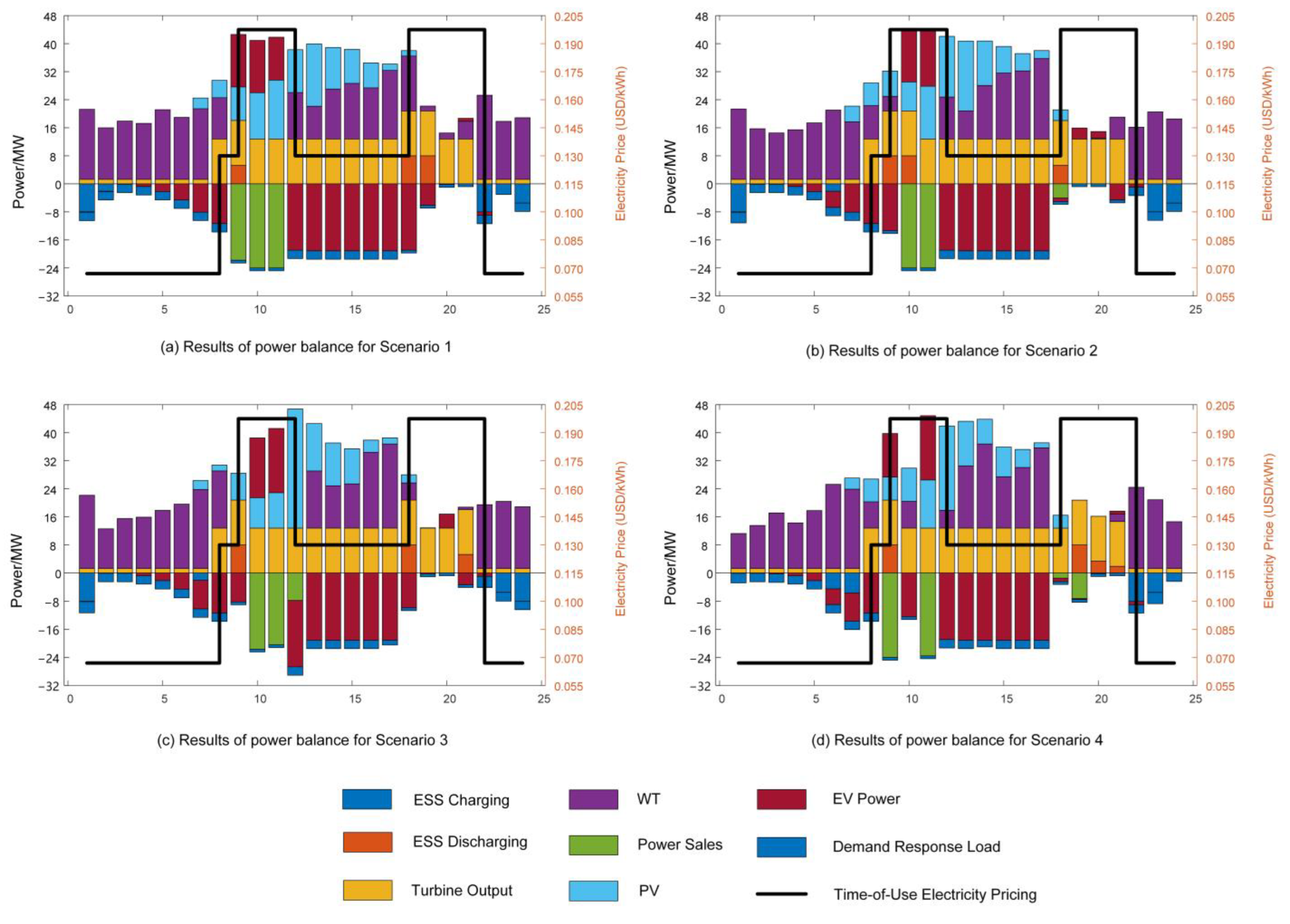
5.2.1. Analysis of Scheduling Results Under Different Scenarios

To validate the proposed optimization scheduling model, this study establishes the following scheduling scenarios:

Scenario 1: The operation and optimization of the microgrid are considered without taking into account load demand response, EVs loads, or the uncertainties associated with wind and solar output.

Scenario 2: Building on Scenario 1, load demand response is incorporated.

Scenario 3: Adding to Scenario 2, EVs electricity load is included.

Scenario 4: Expanding on Scenario 3, wind and solar output uncertainties are integrated, representing the model proposed in this study.

The scheduling results are presented in

Table 3. Scheduling results of four scenarios.

	Revenue (in USD)	Cost (in USD)	Profit (in USD)
Scenario 1	25,362.06	27,175.79	−1813.73
Scenario 2	30,350.17	26,051.30	4298.86
Scenario 3	42,333.98	38,444.69	3889.30
Scenario 4	43,622.96	36,047.70	7575.25

:

As shown in Table 3, Scenario 2 results in a reduction in microgrid operational costs by $1124.49 (approximately a 4.14% decrease) compared to Scenario 1, while total revenue increases by $4988.11 (approximately a 19.67% increase). This suggests that, by incorporating demand response measures––such as peak load demand adjustments, support for renewable energy integration, and enhanced scheduling flexibility––microgrid operations achieve profit maximization.

Scenario 3 builds upon Scenario 2 by adding real-time scheduling for bidirectional charging of EVs. Despite the substantial increase in microgrid electricity demand and a significant rise in operational costs due to EV charging loads, the EV charging and discharging schedule still generates substantial revenue: (1) exploit the peak-valley price difference by charging EVs when electricity prices are low and discharging to the grid when prices are high; (2) V2G technology provides standby services, allowing EVs to quickly supply power in the event of grid failures in exchange for compensation. Consequently, both revenue and costs significantly increase in Scenario 3.

In Scenario 4, compared to Scenario 3, the uncertainty of wind and solar generation profiles is taken into account. Operational costs decrease by $2396.98 (approximately a 6.23% reduction), while total revenues increase by $1288.97 (approximately a 3.04% increase). During periods of high renewable energy generation, the output of the gas turbine per power unit is reduced. Analyzing the volatility and correlation of wind and solar output aids in improving load forecasting, stabilizing load fluctuations, and reducing gas turbine power, thereby achieving cost savings and generating revenue from demand response to some extent. The operational results across different scenarios are illustrated in Figure 8.

From Figure 8, it can be observed that in Scenario 1, the dispatch strategy of the microgrid primarily focuses on optimizing available generation resources, such as traditional steam turbine generation, to ensure stable power supply and economic efficiency within the power system. In this context, the dispatching process is relatively straightforward and can rely directly on deterministic models for energy allocation. However, the microgrid exhibits a lack of flexibility, rendering it inefficient in responding to load fluctuations and changes in the external environment, which may lead to waste of electrical resources and insufficient supply capacity.

In comparison to Scenario 1, Scenario 2 introduces demand response for load management, enabling the microgrid to better adapt to variations in load. By dynamically adjusting the electricity consumption patterns of residential and commercial users––such as encouraging increased electricity demand during lower price periods from 11:00 p.m. to 7:00 a.m. and from 1:00 p.m. to 3:00 p.m.––the flexibility of the microgrid is significantly enhanced. This strategy optimizes the balance between electricity supply and demand, thereby improving the economic performance of the system and increasing the proportion of renewable energy utilization. However, it still does not account for the electricity demand from EVs, which exhibit significant concentrated charging and discharging behavior, leading to considerable fluctuations in grid load.

Building on Scenario 2, Scenario 3 further incorporates the V2G model for electric vehicles. By charging EVs during periods of low grid load and low electricity prices between 1:00 p.m. and 3:00 p.m., this strategy mitigates peak-to-valley fluctuations while enhancing the integration of photovoltaic energy. Additionally, charging is increased during the period of lowest electricity prices and load from 11:00 p.m. to 7:00 a.m. to further smooth these fluctuations and increase wind energy consumption. Furthermore, during other time periods, reverse charging is implemented to meet the load demands of the microgrid and reduce the costs of purchasing electricity. Observations from the figure indicate that this integration not only improves the charging efficiency of electric vehicles but also reduces operational costs for the microgrid, enhancing the adoption of renewable energy.

Scenario 4 considers the uncertainties and complementarity of wind and solar generation output, resulting in more frequent output fluctuations among dispatching units compared to the previous three scenarios. With active responses from distributed energy resources, electric vehicles, and energy users, the consumption of wind and solar power reaches its maximum capacity, effectively controlling the load fluctuations and curtailment associated with the spatiotemporal uncertainties of wind and solar energy.

In addition, as shown in Figure 8, the energy storage devices charge during the early morning low-demand period, primarily achieving the following objectives: (1) Grid Load Balancing: Early morning sees minimal industrial and household activities, resulting in the lowest grid load. Charging during this period helps increase the grid load, thus balancing the grid operation; (2) Optimization of Power System Operation: During low-load periods, the power system may need to reduce or shut down some generators to prevent overvoltage. Charging energy storage devices minimizes such actions and optimizes system operation; (3) Reduction of Electricity Costs: Charging during low-demand periods leverages lower electricity prices, thereby reducing overall energy costs; (4) Support for Renewable Energy Integration: In the early morning, photovoltaic generation is not yet operational, and wind energy is highly variable. Charging can store wind energy and other renewable resources, facilitating their integration; (5) Provision of Flexibility to the Power System: The charged energy storage system can quickly supply power during increased load or generator failures, enhancing system flexibility.

Additionally, the output of gas turbines begins to gradually increase around 8:00 a.m., stabilize around 10:00 a.m., and decrease around 8:00 p.m. This pattern is due to the peak load period between 11:00 a.m. and 3:00 p.m. when photovoltaic generation reaches its maximum. EVs, acting as mobile energy storage, return power to the grid to meet load demand, thereby avoiding additional purchases from the external grid and reducing the gas turbine output, which lowers operational costs.

Furthermore, a phenomenon of concentrated EV charging occurs between 9:00 a.m. and 11:00 a.m. in the microgrid, where the amount of power supplied back to the grid by EVs exceeds the amount drawn from it. This is largely attributed to the microgrid being situated in an industrial and commercial area, which has introduced demand response compensation mechanisms offering higher electricity prices and compensation rates compared to residential areas. EV owners typically complete charging overnight at lower rates and subsequently supplement their consumption with additional charging around 9:00 a.m. This strategy enables them to return energy to the grid in the following hours and obtain demand response benefits.

The load comparison curves before and after demand response optimization are illustrated in Figure 9. It is evident from the figure that the base electric load and EV load are shifted from peak price periods between 10:00–12:00 and 20:00–22:00 to off-peak price periods from 1:00–7:00, as well as flat-rate periods from 8:00–9:00, 13:00–19:00, and 23:00–24:00. This load shift results in a smoother load curve, alleviating pressure on the grid and improving operational efficiency.

Furthermore, the system’s maximum total load decreases from 41.366 MW to 38.523 MW, while the minimum total load increases from 23.163 MW to 23.859 MW. Consequently, the load peak-to-valley difference is optimized from 18.203 MW to 14.664 MW, representing a reduction of 19.44%. These results indicate that the introduction of demand response effectively mitigates load fluctuations and reduces the peak-to-valley difference, establishing a solid foundation for real-time scheduling of EV charging and discharging.

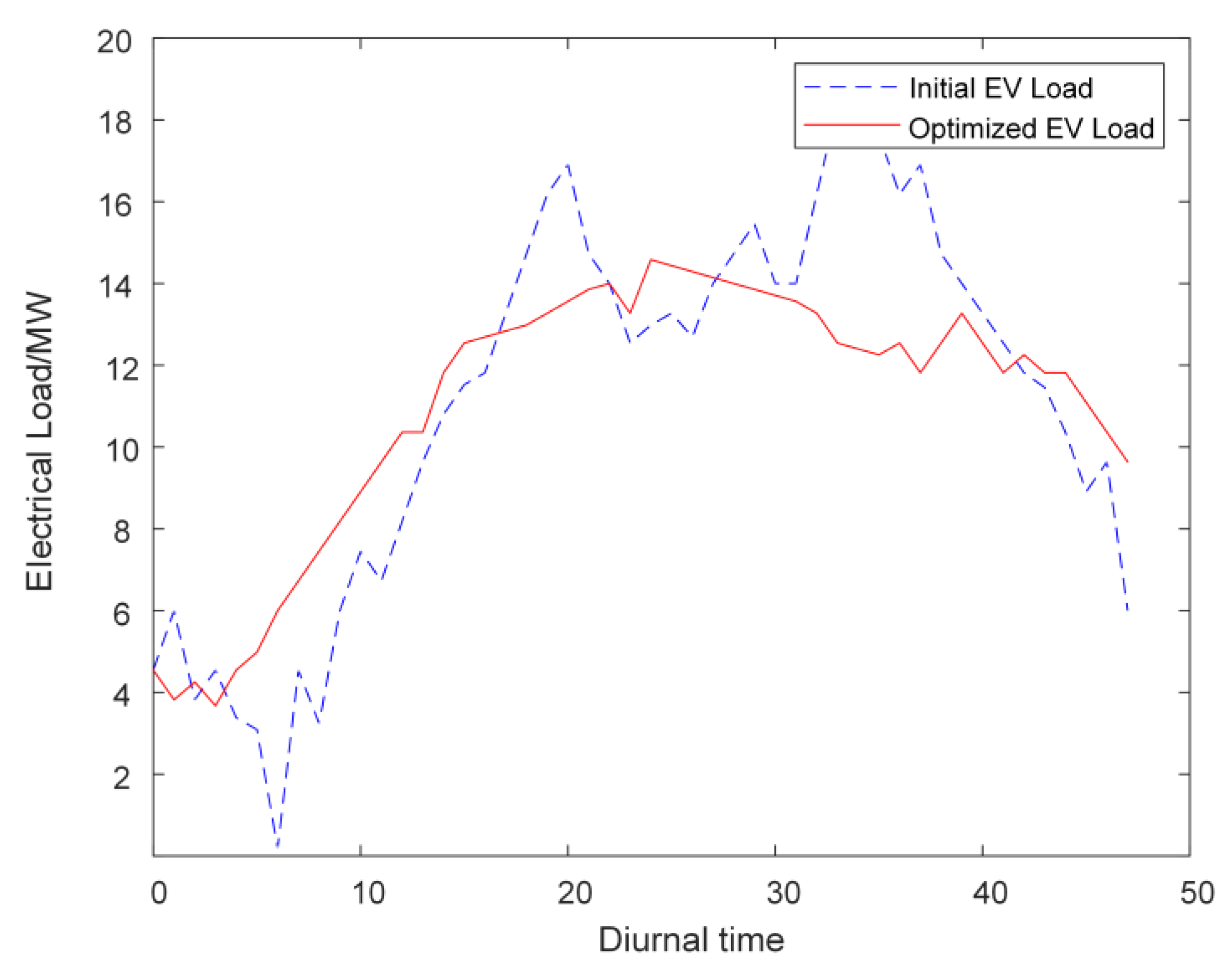
5.2.2. Analysis of Electric Vehicle Charging and Discharging Behavior

Typically, the demand for EV charging increases in the hours leading up to the end of the workday, while EV load remains lower in the morning. Figure 10 illustrates that the base load peaks around 11:00 and 19:00. To avoid charging during high electricity price periods, the scheduling control center seeks to circumvent these peak base load hours. During the significant peak-to-valley differences at 11:00 and 19:00, the EV charging load is negative. The optimized scheduling utilizes V2G technology to discharge EVs during high-price periods, thereby meeting the demand from other electric loads and balancing energy supply and demand. During low-price periods, the scheduling center directs EVs to charge, alleviating pressure on the system and preventing supply constraints during high-load periods, thereby ensuring system stability. For instance, through demand response measures, the charging time for vehicle owners is adjusted from 11:00–16:00 to 9:00–11:00, transforming peak charging hours into reverse charging periods and facilitating the realization of demand response benefits.

The typical daily mileage, charging volume, and charging duration of EVs within the microgrid, generated through Monte Carlo simulation, are shown in Figure 11. It is evident that most EVs charge for under one hour, supporting the idea of concentrating charging during low-load periods, such as at 9:00. Additionally, the total charging volume of about 2 MWh aids in stabilizing the grid load and contributes to peak shaving and valley filling.

Integrating Figure 8, Figure 9, Figure 10 and Figure 11 shows that around 11:00 and 19:00, the discharging activities of V2G-enabled EVs represent a significant share of the overall load, resulting in a total load that is considerably lower than the base load post-scheduling. In contrast, during low-price times, such as 5:00 and 15:00, the scheduling center organizes extensive EV charging, effectively leveraging inexpensive electricity to prepare for upcoming high-demand periods. Real-time scheduling results in the energy consumption of EVs becoming more stabilized, achieving effective peak shaving and valley filling while lowering energy costs associated with charging during high-price intervals.

The experimental findings suggest that the model and optimization scheduling approach introduced in this study have significantly improved the scheduling and operation of microgrids with EVs. This method efficiently aligns the charging and discharging actions of EVs with the energy supply and demand in the microgrid, enabling flexible energy scheduling and distribution while enhancing energy efficiency and the economic performance of the grid.

5.2.3. Sensitivity Analysis

In order to further validate the effectiveness of the model proposed in this paper and to explore the impact of varying numbers of EVs under V2G integration on typical daily load, an unordered charging and discharging pattern, which does not utilize the model introduced in this study, will be used as a control. This analysis will compare the outcomes of ordered charging and discharging scenarios with 50, 100, 150, 200, and 300 EVs integrated into the grid, as illustrated in Figure 12.

Figure 12 illustrates that under the chaotic charging and discharging conditions, without the implementation of the proposed model, the daily load experiences the highest peak-to-valley variation, with load peaks occurring between 9–11 a.m. and 6–8 p.m., while a significant valley is noted from 11 p.m. to 7 a.m. In contrast, utilizing the orderly charging method proposed in this study results in more stable load fluctuations, displaying evident peak-shaving and valley-filling effects. Moreover, as the number of electric vehicles connected to the grid increases from 50 to 200, the load fluctuations within the microgrid become less pronounced, highlighting the pronounced benefits of electric vehicles serving as mobile energy storage. However, beyond 300 grid-connected electric vehicles, there is little improvement in load fluctuations compared to the chaotic charging scenario, with an increase in the peak-to-valley difference. This phenomenon is due to the excessive number of electric vehicles surpassing the microgrid’s capacity to handle additional loads. Therefore, identifying the optimal quantity of electric vehicles that the microgrid can support is essential for ensuring stable operations and enhancing its economic viability.

6. Conclusions

This study utilizes non-parametric kernel density estimation and Frank copula functions to assess the complementarity and uncertainty in wind and solar power generation. By incorporating EVs with V2G technology as mobile storage, a bi-level optimization scheduling model for microgrids is developed. This model aims to minimize operational and environmental costs at the upper level while reducing total energy costs for EVs at the lower level. The key conclusions are as follows:

(1)

The approach using kernel density estimation and Frank copula functions significantly decreases forecasting errors for wind and solar outputs in day-ahead scheduling. This method produces scenarios closely matching actual outputs, enhancing scheduling accuracy and minimizing cost losses from forecast inaccuracies. It provides a solid foundation for power system operations and market transactions, improving demand response and facilitating the integration of renewable energy.

(2)

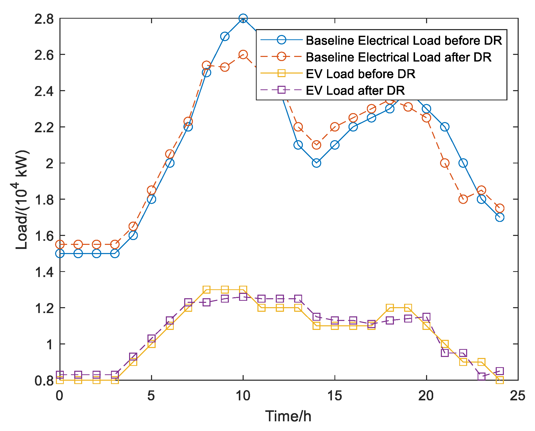
The integration of comprehensive demand response leads to a reduction in the microgrid’s maximum total load from 41.366 MW to 38.523 MW, while the minimum total load rises from 23.163 MW to 23.859 MW, optimizing the load peak-to-valley difference to 14.664 MW, a decrease of 19.44%. The effects of comprehensive demand response contribute to stabilizing load fluctuations, establishing a robust basis for real-time scheduling of EV charging and discharging.

(3)

The bi-level optimization scheduling model presented in this paper, which integrates V2G technology, effectively synchronizes the charging and discharging activities of EVs with the microgrid’s energy supply and demand. The orderly EV charging strategy adopted after scheduling substantially diminishes grid load fluctuations, enabling peak shaving and valley filling. This flexibility enhances energy scheduling and distribution, ultimately improving the energy efficiency and economic sustainability of the grid.

7. Future Research Outlook

The strategy proposed in this paper does not take into account the interaction scenarios among multiple microgrids. Future research plans to further explore the joint scheduling strategies for V2G systems involving massive electric vehicle integration across multiple microgrids. Additionally, studying the integration of other renewable energy sources, larger-scale microgrid systems, and coordinated scheduling across multiple time scales would be feasible and beneficial, providing valuable guidance for practical applications.

References

1. Li, J.D.; Chen, S.J.; Wu, Y.Q.; Wang, Q.H.; Liu, X.; Qi, L.J.; Lu, X.Y.; Gao, L. How to make better use of intermittent and variable energy? A review of wind and photovoltaic power consumption in China. Renew. Sustain. Energy Rev. 2021, 137, 110626. [Google Scholar] [CrossRef]
2. Li, Z.L.; Li, P.; Yuan, Z.P.; Xia, J.; Tian, D. Optimized utilization of distributed renewable energies for island microgrid clusters considering solar-wind correlation. Electr. Power Syst. Res. 2022, 206, 107822. [Google Scholar] [CrossRef]
3. Yu, H.; Niu, S.Y.; Shang, Y.T.; Shao, Z.Y.; Jia, Y.W.; Jian, L.N. Electric vehicles integration and vehicle-to-grid operation in active distribution grids: A comprehensive review on power architectures, grid connection standards and typical applications. Renew. Sustain. Energy Rev. 2022, 168, 112812. [Google Scholar] [CrossRef]
4. Hoicka, C.E.; Rowlands, I.H. Solar and wind resource complementarity: Advancing options for renewable electricity integration in Ontario, Canada. Renew. Energy 2011, 36, 97–107. [Google Scholar] [CrossRef]
5. Lin, S.F.; Liu, C.T.; Shen, Y.W.; Li, F.X.; Li, D.D.; Fu, Y. Stochastic Planning of Integrated Energy System via Frank-Copula Function and Scenario Reduction. IEEE Trans. Smart Grid 2022, 13, 202–212. [Google Scholar] [CrossRef]
6. Li, K.; Duan, P.F.; Xue, Q.W.; Cheng, Y.D.; Hua, J.; Chen, J.L.; Guo, P.H. Enhancing reliability assessment in distributed generation networks: Incorporating dynamic correlation of wind-solar power output uncertainty. Sustain. Energy Grids Netw. 2024, 39, 101505. [Google Scholar] [CrossRef]
7. Wang, Q.; Zhang, X.G.; Yi, C.Z.; Li, Z.B.; Xu, D.G. A Novel Shared Energy Storage Planning Method Considering the Correlation of Renewable Uncertainties on the Supply Side. IEEE Trans. Sustain. Energy 2022, 13, 2051–2063. [Google Scholar] [CrossRef]
8. Zhao, M.Z.; Wang, Y.M.; Wang, X.B.; Chang, J.X.; Zhou, Y.; Liu, T. Modeling and Simulation of Large-Scale Wind Power Base Output Considering the Clustering Characteristics and Correlation of Wind Farms. Front. Energy Res. 2022, 10, 810082. [Google Scholar] [CrossRef]
9. Zhou, H.; Wu, H.H.; Ye, C.J.; Xiao, S.J.; Zhang, J.; He, X.; Wang, B. Integration Capability Evaluation of Wind and Photovoltaic Generation in Power Systems Based on Temporal and Spatial Correlations. Energies 2019, 12, 171. [Google Scholar] [CrossRef]
10. Ru, Y.; Wang, Y.; Mao, W.J.; Zheng, D.; Fang, W.Q. Dynamic Environmental Economic Dispatch Considering the Uncertainty and Correlation of Photovoltaic-Wind Joint Power. Energies 2024, 17, 6247. [Google Scholar] [CrossRef]
11. Sun, L.; Xu, Q.S.; Chen, X.; Fan, Y.K. Day-ahead economic dispatch of microgrid based on game theory. Energy Rep. 2020, 6, 633–638. [Google Scholar] [CrossRef]
12. Leng, C.M.; Yang, H.; Song, Y.K.; Yu, Z.T.; Shen, C. Expected value model of microgrid economic dispatching considering wind power uncertainty. Energy Rep. 2023, 9, 291–298. [Google Scholar] [CrossRef]
13. Huo, Y.C.; Bouffard, F.; Joós, G. Decision tree-based optimization for flexibility management for sustainable energy microgrids. Appl. Energy 2021, 290, 116772. [Google Scholar] [CrossRef]
14. Du, X.D.; Wang, L.B.; Zhao, J.L.; He, Y.L.; Sun, K. Power Dispatching of Multi-Microgrid Based on Improved CS Aiming at Economic Optimization on Source-Network-Load-Storage. Electronics 2022, 11, 2742. [Google Scholar] [CrossRef]
15. He, Y.L.; Wu, X.W.; Sun, K.; Liu, X.Y.; Wang, H.P.; Zeng, S.M.; Zhang, Y. A Novel MOWSO algorithm for Microgrid multi-objective optimal dispatch. Electr. Power Syst. Res. 2024, 232, 110374. [Google Scholar] [CrossRef]
16. Lei, X.; Huang, T.; Yang, Y.; Fang, Y.; Wang, P. A Bi-Layer Multi-Time Coordination Method for Optimal Generation and Reserve Schedule and Dispatch of a Grid-Connected Microgrid. IEEE Access 2019, 7, 44010–44020. [Google Scholar] [CrossRef]
17. Du, J.L.; Hu, W.H.; Zhang, S.; Liu, W.; Zhang, Z.Y.; Wang, D.J.; Chen, Z. A multi-objective robust dispatch strategy for renewable energy microgrids considering multiple uncertainties. Sustain. Cities Soc. 2024, 116, 105918. [Google Scholar] [CrossRef]
18. Jiang, H.Y.; Ning, S.Y.; Ge, Q.B. Multi-Objective Optimal Dispatching of Microgrid With Large-Scale Electric Vehicles. IEEE Access 2019, 7, 145880–145888. [Google Scholar] [CrossRef]
19. Hakimi, S.M.; Moghaddas-Tafreshi, S.M. Effect of plug-in hybrid electric vehicles charging/discharging management on planning of smart microgrid. J. Renew. Sustain. Energy 2012, 4, 063144. [Google Scholar] [CrossRef]
20. Wu, T.; Yang, Q.; Bao, Z.J.; Yan, W.J. Coordinated Energy Dispatching in Microgrid With Wind Power Generation and Plug-in Electric Vehicles. IEEE Trans. Smart Grid 2013, 4, 1453–1463. [Google Scholar] [CrossRef]
21. Shi, R.F.; Li, S.P.; Zhang, P.H.; Lee, K.Y. Integration of renewable energy sources and electric vehicles in V2G network with adjustable robust optimization. Renew. Energy 2020, 153, 1067–1080. [Google Scholar] [CrossRef]
22. Zhang, X.Z.; Wang, Z.Y.; Lu, Z.Y. Multi-objective load dispatch for microgrid with electric vehicles using modified gravitational search and particle swarm optimization algorithm. Appl. Energy 2022, 306, 118018. [Google Scholar] [CrossRef]
23. Wu, J.Q.; Zhang, Q.; Lu, Y.D.; Qin, T.X.; Bai, J.Y. Source-Load Coordinated Low-Carbon Economic Dispatch of Microgrid including Electric Vehicles. Sustainability 2023, 15, 15287. [Google Scholar] [CrossRef]
24. Luo, Z.J.; Ren, H.; Xin, G.Y.; Xu, M.K.; Wang, F.; Zhang, Y.C. Optimal operation of microgrid with consideration of V2G’s uncertainty. Iet Gener. Transm. Distrib. 2024, 18, 289–302. [Google Scholar] [CrossRef]
25. Wang, Y.Q.; Guo, X.Z.; Zhang, C.; Liang, R.; Peng, T.; Yang, Y.; Wu, M.J.; Zhou, Y.X. Multi-strategy reference vector guided evolutionary algorithm and its application in multi-objective optimal scheduling of microgrid systems containing electric vehicles. J. Energy Storage 2024, 95, 112500. [Google Scholar] [CrossRef]
26. Yu, J.; Feng, Q.Z.; Li, Y.; Cao, J.D. Stochastic Optimal Dispatch of Virtual Power Plant considering Correlation of Distributed Generations. Math. Probl. Eng. 2015, 2015, 135673. [Google Scholar] [CrossRef]
27. Zhang, Y.; Wang, J.X.; Wang, X.F. Review on probabilistic forecasting of wind power generation. Renew. Sustain. Energy Rev. 2014, 32, 255–270. [Google Scholar] [CrossRef]
28. Semeyutin, A.; O’Neill, R. A brief survey on the choice of parameters for: “Kernel density estimation for time series data”. N. Am. J. Econ. Financ. 2019, 50, 101038. [Google Scholar] [CrossRef]
Figure 1. Microgrid Architecture.
Energies 18 00823 g001
Figure 2. Scenario Reduction Process Based on the Backward Elimination Method.
Energies 18 00823 g002
Figure 3. Flowchart of microgrid optimal scheduling.
Energies 18 00823 g003
Figure 4. Optimization range of EV charging/discharging periods.
Energies 18 00823 g004
Figure 5. Flow chart of lower EV charge/discharge optimization scheduling.
Energies 18 00823 g005
Figure 6. Generation and reduction of landscape scene. (a) Consider 500 scenarios of wind power generation output generated based on correlations; (b) Consider 500 scenarios of photovoltaic output generated based on correlation analysis; (c) Five scenarios of reduced wind power output; (d) Five scenarios of reduced photovoltaic output.
Energies 18 00823 g006
Figure 7. Total EV load.
Energies 18 00823 g007
Figure 8. Results of different scenarios.
Energies 18 00823 g008
Figure 9. Load comparison before and after microgrid demand response.
Energies 18 00823 g009
Figure 10. Lower EV load optimization results.
Energies 18 00823 g010
Figure 11. Generation of mileage, charge, and charge duration for a typical day of electric vehicle driving based on Monte Carlo method.
Energies 18 00823 g011
Figure 12. Comparison of the Impact of Different Charging and Discharging Modes and the Number of Grid-Connected Vehicles on Typical Daily Load.
Energies 18 00823 g012