
Energy Scheduling Strategy for the Gas–Steam–Power System in Steel Enterprises Under the Influence of Time-Of-Use Tariff

Abstract
1. Introduction
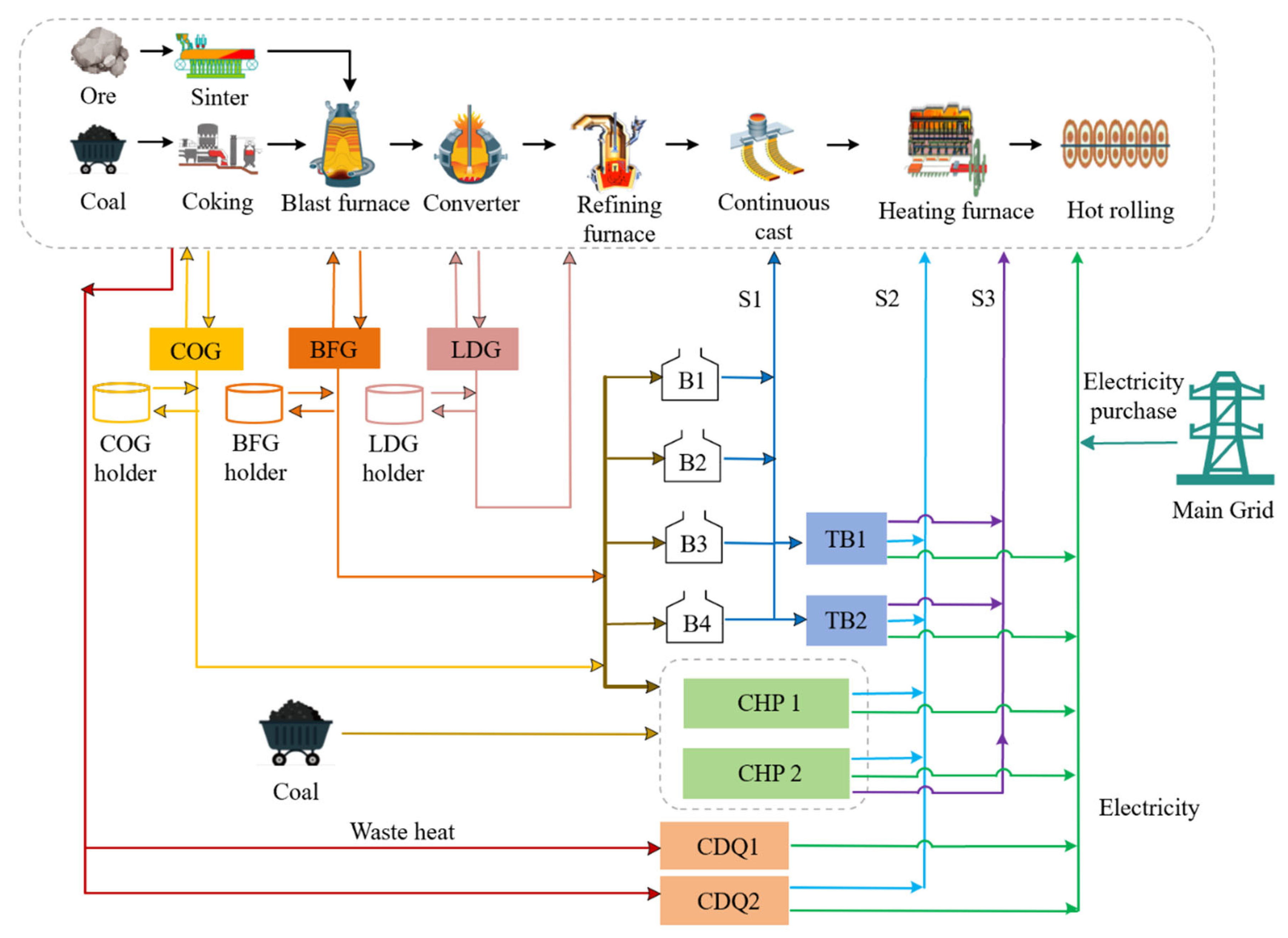
2. Problem Statement
3. Mathematical Model
- A.
- Steam and Power Generation Model
- (1)
- Boilers
Steam Turbines
- (2)
- CHP
- (3)
- CDQ
- B.
- Gas, Steam, and Power Balances
- C.
- Gas Holder Operational Model
- D.
- Burner Operational Constraints
- E.
- Objective Function
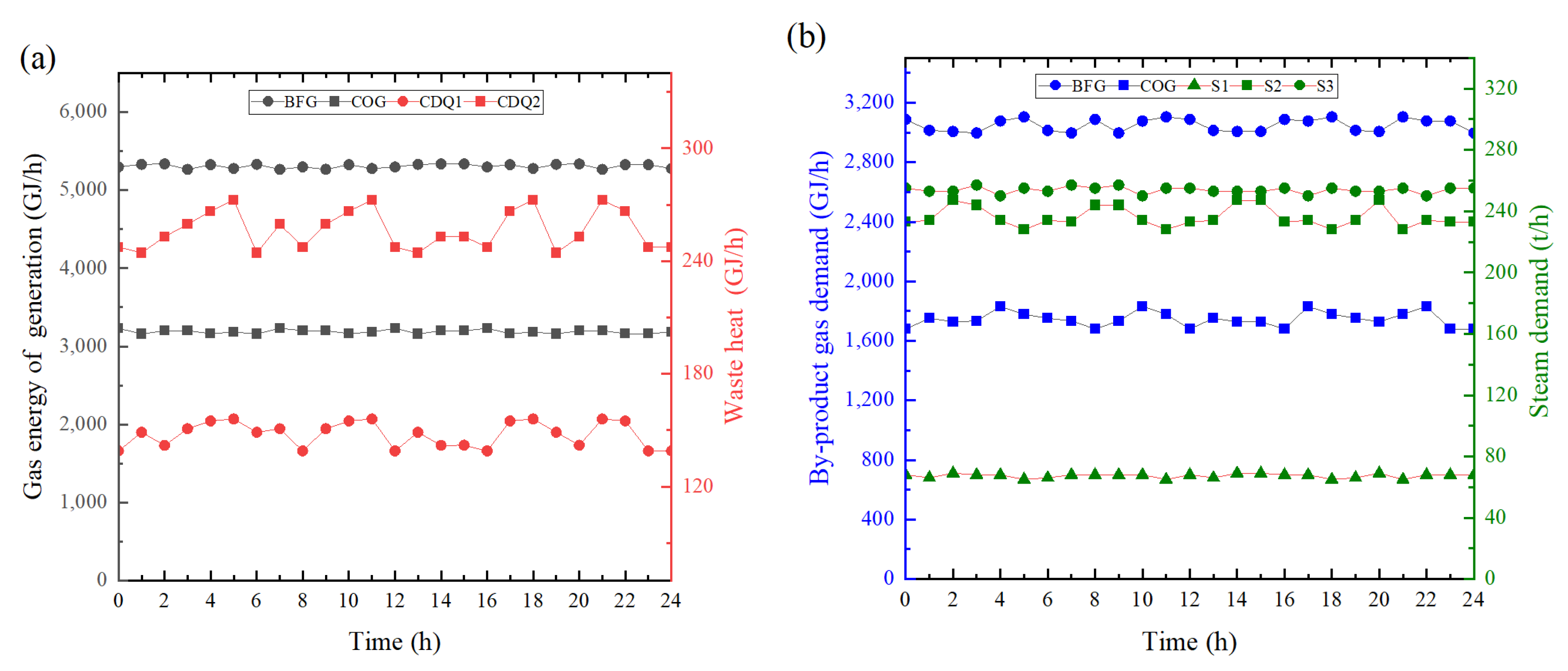
4. Case Study
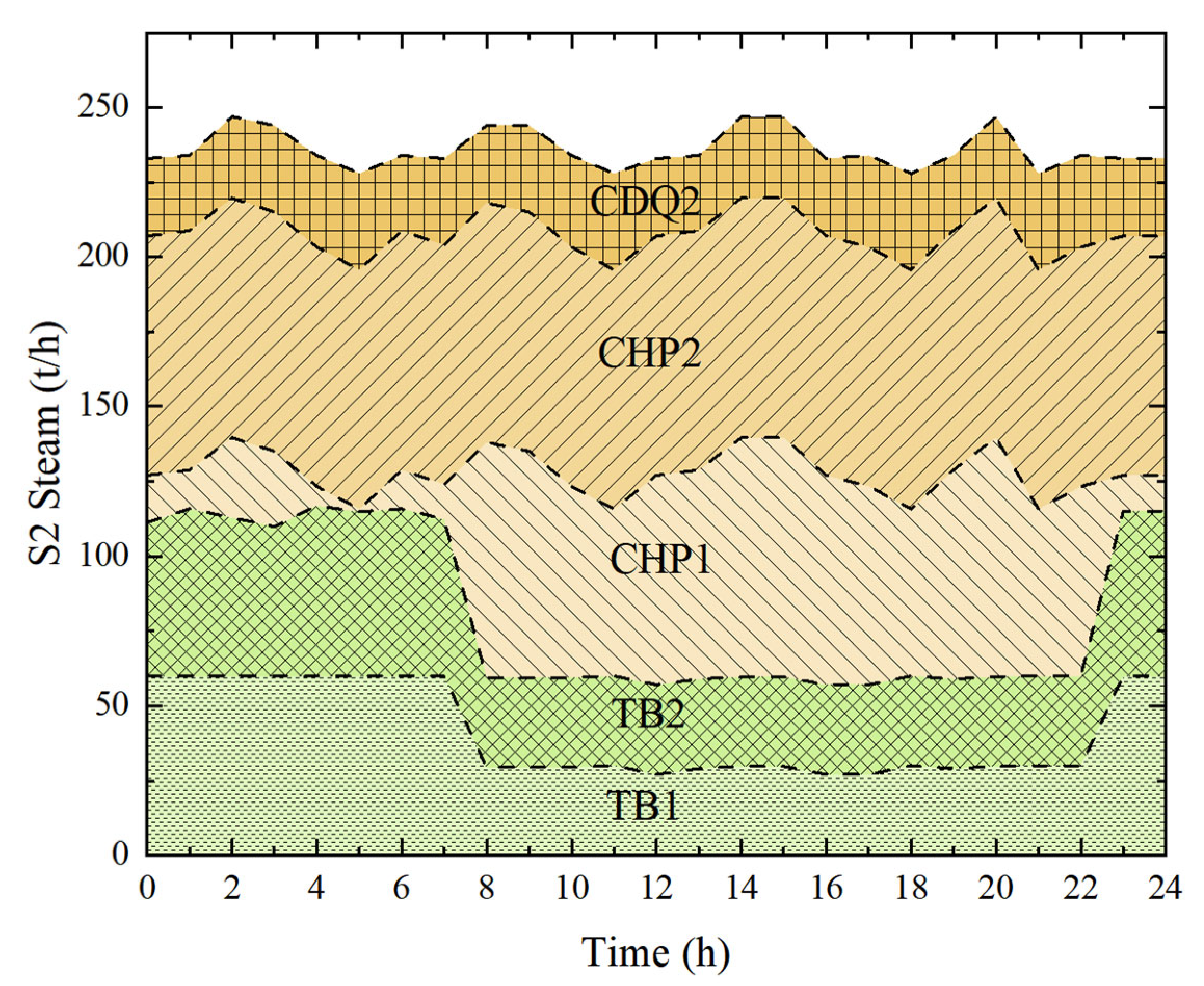
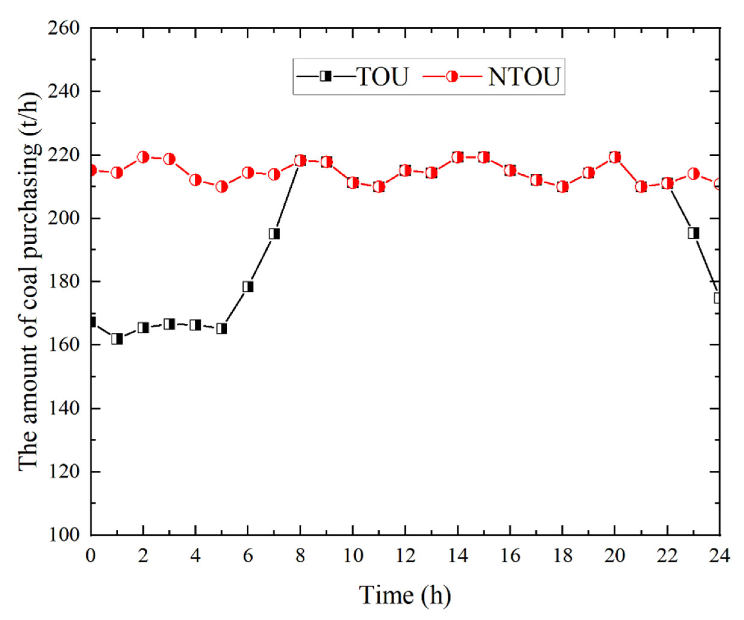
5. Results and Discussions
6. Conclusions
Author Contributions
Funding
Data Availability Statement
Conflicts of Interest
Correction Statement
Nomenclature
| t | period |
| R | steam |
| J | steam turbine |
| K | CHP unit |
| M | CDQ unit |
| Qg | different types of gases |
| Sirt | flow rate of steam, ton/h |
| feedwater flow rate of boiler, ton/h | |
| Viqt | feed flow rate of fuel q, km3/h |
| η | thermal efficiency of boiler |
| hvq | heating value of fuels |
| h | enthalpy |
| Sjt | steam flow of the steam turbine, ton/h |
| Sjrt | flow of grade r steam of the steam turbine, ton/h |
| fj,t | power generation of steam turbine, MW/h |
| fkt | power output of CHP, MW/h |
| Skrt | flow rate of steam, ton/h |
| fmt | power generation of the CDQ, MW/h |
| total waste heat recovered by the CDQ, GJ/h | |
| demand for power, MW | |
| electricity purchase, MW | |
| electricity sales, MW | |
| steam demand, km3 | |
| y | costs |
| generation rate of gas, km3/h | |
| Vqtu | consumption rate of gas, km3/h |
| Qemission | flaring amount of gas, km3 |
| DR | demand response |
| GSPS | gas–steam–power system |
| TOU | time-of-use |
| MILP | mixed-integer linear programming |
| CDQ | coke dry quenching |
| NTOU | not time-of-use |
| CHP | combined heat and power |
| COG | gas recovered from the coking process |
| BFG | gas recovered from blast furnace |
| LDG | gas recovered from the converter process |
Appendix A

| Boiler | Efficiency (ηi) | (m3/h) | (m3/h) | (t/h) | (t/h) | (GJ/m3) |
|---|---|---|---|---|---|---|
| B1 | 0.89 | 40 | 6 | 0 | 35 | 0.0035 |
| B2 | 0.92 | 40 | 6 | 0 | 35 | 0.0035 |
| B3 | 0.84 | 120 | 7 | 0 | 130 | 0.0035 |
| B4 | 0.86 | 120 | 7 | 0 | 130 | 0.0035 |
| Boilers | Initial Number | Inlet Flow Rate per Burner (m3/h) | ||
|---|---|---|---|---|
| COG | BFG | COG | BFG | |
| B1 | 2 | 4 | 0.5 | 5 |
| B2 | 2 | 4 | 0.5 | 5 |
| B3 | 0 | 23 | 0.5 | 5 |
| B4 | 0 | 23 | 0.5 | 5 |
| CHP1 | 14 | 16 | 2 | 10 |
| CHP2 | 14 | 16 | 2 | 10 |
| Volume | COG | BFG | LDG |
|---|---|---|---|
| Minimum capacity (m3) | 40 | 50 | 15 |
| Low operational inventory level (m3) | 80 | 140 | 25 |
| Normal operational inventory level (m3) | 100 | 180 | 40 |
| High operational inventory level (m3) | 120 | 220 | 55 |
| Maximum capacity (m3) | 135 | 260 | 70 |
| COG (GJ/m3) | BFG (GJ/m3) | LDG (GJ/m3) | Coal | |
|---|---|---|---|---|
| Calorific value | 0.018 | 0.0035 | 0.0075 | 0.0218 |
| Item | Boiler feed water (GJ/kg) | S1 (GJ/kg) | S2 (GJ/kg) | S3 (GJ/kg) |
| Enthalpy | 0.00010538 | 0.0033 | 0.0031 | 0.00293 |
| Parameters | Value |
|---|---|
| Maximum imported power (MW) | 130 |
| Maximum exported power (MW) | 100 |
| Penalty coefficient for gas emission (¥/m3) | 100 |
| Penalty coefficient for violation of high operational level (¥/m3) | 10 |
| Penalty coefficient for violation of low operational level (¥/m3) | 5 |
| Penalty coefficient for burner switches (¥/switch) | 800 |
| Penalty coefficient for simultaneous switches of two burners (¥/instance) | 100 |
| Penalty coefficient for simultaneous switches of three burners (¥/instance) | 200 |
| Maintenance cost of boilers (¥/t) | 6 |
| Maintenance cost of turbines (¥/kWh) | 0.06 |
| Maintenance cost of CHP units (¥/kWh) | 0.08 |
| Maintenance cost of CDQ units(¥/kWh) | 0.06 |
| Coal purchase cost (¥/t) | 500 |
| Electricity sale price (¥/kWh) | 0.2 |
| TB | Efficiency (ηj) | (t/h) | (t/h) | (t/h) | (t/h) | (t/h) | (t/h) | (MW) | (MW) | DRj (MW/h) | URj (MW/h) |
|---|---|---|---|---|---|---|---|---|---|---|---|
| TB1 | 0.82 | 60 | 130 | 0 | 60 | 0 | 100 | 0 | 25 | 5 | 5 |
| TB2 | 0.85 | 60 | 130 | 0 | 60 | 0 | 100 | 0 | 25 | 5 | 5 |
| CDQ | Efficiency (ηm) | (t/h) | (t/h) | (t/h) | (t/h) | (MW) | (MW) | DRm (MW/h) | URm (MW/h) |
|---|---|---|---|---|---|---|---|---|---|
| CDQ1 | 0.73 | 0 | 40 | 0 | 60 | 0 | 30 | 5 | 5 |
| CDQ2 | 0.75 | 0 | 40 | 0 | 60 | 0 | 30 | 5 | 5 |
| CHP | Efficiency (ηk) | (m3/h) | (m3/h) | (GJ/m3) | (t/h) | (t/h) | (t/h) | (t/h) | (MW) | (MW) | DRk (MW/h) | URk (MW/h) |
|---|---|---|---|---|---|---|---|---|---|---|---|---|
| CHP1 | 0.38 | 0 | 130 | 0.0046 | 0 | 80 | 0 | 110 | 220 | 300 | 20 | 20 |
| CHP2 | 0.39 | 0 | 130 | 0.0046 | 0 | 80 | 0 | 110 | 220 | 300 | 20 | 20 |
| Period | Gases (m3/h) | CDQ (GJ) | Power (MW) | Steam (t/h) | |||||
|---|---|---|---|---|---|---|---|---|---|
| BFG | COG | LDG | CDQ1 | CDQ2 | S1 | S2 | S3 | ||
| 0 | 1514 | 179.50 | 47 | 138.965 | 247.400 | 698 | 68 | 233 | 255 |
| 1 | 1523 | 175.50 | 46 | 138.965 | 244.365 | 690 | 66 | 234 | 253 |
| 2 | 1525 | 177.70 | 45 | 138.965 | 252.940 | 685 | 69 | 247 | 253 |
| 3 | 1505 | 177.80 | 45 | 138.965 | 259.550 | 691 | 68 | 244 | 257 |
| 4 | 1522 | 175.70 | 49 | 138.965 | 266.540 | 707 | 68 | 234 | 250 |
| 5 | 1508 | 176.80 | 38 | 138.965 | 272.540 | 709 | 65 | 228 | 255 |
| 6 | 1523 | 175.50 | 47 | 138.965 | 244.367 | 690 | 66 | 234 | 253 |
| 7 | 1505 | 179.50 | 46 | 138.965 | 259.549 | 691 | 68 | 233 | 257 |
| 8 | 1514 | 177.80 | 45 | 138.965 | 247.403 | 698 | 68 | 244 | 255 |
| 9 | 1505 | 177.80 | 45 | 138.965 | 259.555 | 691 | 68 | 244 | 257 |
| 10 | 1522 | 175.70 | 49 | 138.965 | 266.537 | 707 | 68 | 234 | 250 |
| 11 | 1508 | 176.80 | 38 | 138.965 | 272.542 | 709 | 65 | 228 | 255 |
| 12 | 1514 | 179.50 | 47 | 138.965 | 247.403 | 698 | 68 | 233 | 255 |
| 13 | 1523 | 175.50 | 46 | 138.965 | 244.363 | 690 | 66 | 234 | 253 |
| 14 | 1525 | 177.70 | 45 | 138.965 | 252.937 | 685 | 69 | 247 | 253 |
| 15 | 1525 | 177.70 | 45 | 138.965 | 252.942 | 685 | 69 | 247 | 253 |
| 16 | 1514 | 179.50 | 49 | 138.965 | 247.396 | 698 | 68 | 233 | 255 |
| 17 | 1522 | 175.70 | 38 | 138.965 | 266.542 | 707 | 68 | 234 | 250 |
| 18 | 1508 | 176.80 | 47 | 138.965 | 272.536 | 709 | 65 | 228 | 255 |
| 19 | 1523 | 175.50 | 46 | 138.965 | 244.371 | 690 | 66 | 234 | 253 |
| 20 | 1525 | 177.70 | 45 | 138.965 | 252.942 | 685 | 69 | 247 | 253 |
| 21 | 1505 | 177.80 | 38 | 138.965 | 272.538 | 709 | 65 | 228 | 255 |
| 22 | 1522 | 175.70 | 38 | 138.965 | 266.543 | 707 | 68 | 234 | 250 |
| 23 | 1522 | 175.70 | 49 | 138.965 | 247.399 | 698 | 68 | 233 | 255 |
| 24 | 1508 | 176.80 | 45 | 138.965 | 247.404 | 698 | 68 | 233 | 255 |
References
- Notice of the Ministry of Industry and Information Technology of the People’s Republic of China on the Release of Energy Efficiency Benchmark Levels and Benchmark Levels in Key Areas of High Energy Consuming Industries (2021 Edition) by Five Departments. 15 November 2021. Available online: https://www.miit.gov.cn (accessed on 22 June 2023).
- Shahabuddin, M.; Brooks, G.; Rhamdhani, M.A. Decarbonisation and hydrogen integration of steel industries: Recent development, challenges and technoeconomic analysis. J. Clean. Prod. 2023, 395, 136391. [Google Scholar] [CrossRef]
- Watari, T.; McLellan, B. Global demand for green hydrogen-based steel: Insights from 28 scenarios. Int. J. Hydrogen Energy 2024, 79, 630–635. [Google Scholar] [CrossRef]
- Zhang, J.; Shen, J.; Xu, L.; Zhang, Q. The CO2 emission reduction path towards carbon neutrality in the Chinese steel industry: A review. Environ. Impact Assess. Rev. 2023, 99, 107017. [Google Scholar] [CrossRef]
- Li, W.; Zhang, S.; Lu, C. Research on the driving factors and carbon emission reduction pathways of China’s iron and steel industry under the vision of carbon neutrality. J. Clean. Prod. 2022, 361, 132237. [Google Scholar] [CrossRef]
- Lin, B.; Wu, R. Designing energy policy based on dynamic change in energy and carbon dioxide emission performance of China’s iron and steel industry. J. Clean. Prod. 2020, 256, 120412. [Google Scholar] [CrossRef]
- Ren, L.; Zhou, S.; Peng, T.; Ou, X. A review of CO2 emissions reduction technologies and low-carbon development in the iron and steel industry focusing on China. Renew. Sustain. Energy Rev. 2021, 143, 110846. [Google Scholar] [CrossRef]
- Zhang, Q.; Di, W.; Du, T.; Cai, J. Coupling Model of Surplus Gas-Steam-Electricity and Its Application in Steel Enterprises. CIESC J. 2011, 62, 753–758. [Google Scholar]
- Xu, T.; Huo, Z.; Wang, W.; Xie, N.; Li, L.; Liu, Y.; Mu, L. Evaluation of by-product-gas utilization options for carbon reduction at an integrated iron and steel mill. Energy 2024, 294, 130959. [Google Scholar] [CrossRef]
- Branca, T.A.; Colla, V.; Algermissen, D.; Granbom, H.; Martini, U.; Morillon, A.; Pietruck, R.; Rosendahl, S. Reuse and recycling of by-products in the steel sector: Recent achievements paving the way to circular economy and industrial symbiosis in Europe. Metals 2020, 10, 345. [Google Scholar] [CrossRef]
- Sui, P.; Ren, B.; Wang, J.; Wang, G.; Zuo, H.; Xue, Q. Current situation and development prospects of metallurgical by-product gas utilization in China’s steel industry. Int. J. Hydrog. Energy 2023, 48, 28945–28969. [Google Scholar] [CrossRef]
- Zhang, Q.; Zhao, X.; Lu, H.; Ni, T.; Li, Y. Waste energy recovery and energy efficiency improvement in China’s iron and steel industry. Appl. Energy 2017, 191, 502–520. [Google Scholar] [CrossRef]
- Si, M. The Feasibility of Waste Heat Recovery and Energy Efficiency Assessment in a Steel Plant. Master’s Thesis, University of Manitoba, Winnipeg, MB, Canada, 2011. [Google Scholar]
- Liu, J.; Chang, Y. Research on Models of Power Production in Integrated Iron and Steel Factory. J. Northeast. Univ. (Nat. Sci.) 2014, 35, 1719. [Google Scholar]
- Hu, Z.; He, D. Operation scheduling optimization of gas–steam–power conversion systems in iron and steel enterprises. Appl. Therm. Eng. 2022, 206, 118121. [Google Scholar] [CrossRef]
- Supply, T.P. Demand response potential assessment of steel plant based on refined simulation. Methods 2023, 24, 25. [Google Scholar]
- Masebinu, R.O. Assessing the Potential for Flexible Demand-Side Management in the Steel Industrial Sector in South Africa. Master’s Thesis, University of Johannesburg, Johannesburg, South Africa, 2021. [Google Scholar]
- Yuan, Y.; Na, H.; Chen, C.; Qiu, Z.; Sun, J.; Zhang, L.; Du, T.; Yang, Y. Status, Challenges, and Prospects of Energy Efficiency Improvement Methods in Steel Production: A Multi-Perspective Review. Energy 2024, 304, 132047. [Google Scholar] [CrossRef]
- Ming, D.; Li, J.; Yin, Y. Optimization Scheduling Model Study for Coke Oven Gas in Steel Companies. Comput. Eng. Des. 2008, 6, 1575–1578. [Google Scholar]
- Zhang, X.; Zhang, Y.; Tang, L. Optimization Model for the Blending and Allocation of Coke Oven Gas in Steel Enterprises. J. Syst. Eng. 2011, 26, 710–717. [Google Scholar]
- Chen, J.; Zhou, W.; Wang, H. Study on optimal multi-period operational strategy for steam power system in steel industry. Chem. Ind. Eng. Prog. 2017, 36, 1589–1596. [Google Scholar]
- Li, J. Optimization Scheduling of the Steam System in Steel Enterprises. Master’s Thesis, Tianjin University of Technology, Tianjin, China, 2016. [Google Scholar]
- Hao, F.; Gao, Q.; Jiang, B.; Chen, G. Research and Application of Intelligent Power Dispatching Integrated System in Steel Enterprises. Metall. Ind. Autom. 2013, 37, 33–38. [Google Scholar]
- Ma, G. Analysis and Optimization Research of Power Systems in Integrated Steel Enterprises. Master’s Thesis, Northeastern University, Boston, MA, USA, 2014. [Google Scholar]
- Akimoto, K.; Sannomiya, N.; Nishikawa, Y.; Tsuda, T. An optimal gas supply for a power plant using a mixed interger programming model. Utomatic 1991, 27, 513–518. [Google Scholar]
- Zhao, X.; Bai, H.; Lu, X.; Shi, Q.; Han, J. A MILP model concerning the optimisation of penalty factors for the short-term distribution of byproduct gases produced in the iron and steel making process. Appl. Energy 2015, 148, 142–158. [Google Scholar] [CrossRef]
- García García, S.; Rodríguez Montequín, V.; Morán Palacios, H.; Mones Bayo, A. A mixed integer linear programming model for the optimization of steel waste gases in cogeneration: A combined coke oven and converter gas case study. Energies 2020, 13, 3781. [Google Scholar] [CrossRef]
- Kong, H.; Qi, E.; Li, H.; Li, G.; Zhang, X. An MILP model for optimization of byproduct gases in the integrated iron and steel plant. Appl. Energy 2010, 87, 2156–2163. [Google Scholar] [CrossRef]
- Jiang, S.L.; Wang, M.; Bogle, I.D.L. Plant-wide byproduct gas distribution under uncertainty in iron and steel industry via quantile forecasting and robust optimization. Appl. Energy 2023, 350, 121603. [Google Scholar] [CrossRef]
- Shu, Y. Research on the Synergy Scheduling of Coke Oven Gas, Steam, and Electricity in Steel Enterprises. Master’s Thesis, Chongqing University, Chongqing, China, 2020. [Google Scholar]
- He, D.; Lu, X.; Feng, K.; Xu, A. Coupling Optimization Scheduling of Coke Oven Gas-Steam-Electricity System in Steel Enterprises. Steel 2018, 53, 95–104. [Google Scholar]
- He, D.; Liu, P.; Feng, K.; Xu, A. Collaborative optimization of rolling plan and energy dispatching in steel plants. China Metall. 2019, 29, 75–80. [Google Scholar]
- Zhao, X.; Bai, H.; Shi, Q.; Lu, X.; Zhang, Z. Optimal scheduling of a byproduct gas system in a steel plant considering time-of-use electricity pricing. Appl. Energy 2017, 195, 100–113. [Google Scholar] [CrossRef]
- Liu, S.; Xie, S.; Zhang, Q. Multi-energy synergistic optimization in steelmaking process based on energy hub concept. Int. J. Miner. Metall. Mater. 2021, 28, 1378–1386. [Google Scholar] [CrossRef]
- Zhao, J.; Wang, W.; Sun, K.; Liu, Y. A Bayesian networks structure learning and reasoning-based byproduct gas scheduling in steel industry. IEEE Trans. Autom. Sci. Eng. 2013, 11, 1149–1154. [Google Scholar] [CrossRef]
- Aguilar, O.; Perry, S.J.; Kim, J.K.; Smith, R. Design and optimization of flexible utility systems subject to variable conditions: Part 1: Modelling framework. Chem. Eng. Res. Des. 2007, 85, 1136–1148. [Google Scholar] [CrossRef]
- Mitra, S.; Sun, L.; Grossmann, I.E. Optimal scheduling of industrial combined heat and power plants under time-sensitive electricity prices. Energy 2013, 54, 194–211. [Google Scholar] [CrossRef]
- Bischi, A.; Taccari, L.; Martelli, E.; Amaldi, E.; Manzolini, G.; Silva, P.; Campanari, S.; Macchi, E. A detailed MILP optimization model for combined cooling, heat and power system operation planning. Energy 2014, 74, 12–26. [Google Scholar] [CrossRef]
- Zeng, Y.; Xiao, X.; Li, J.; Sun, L.; Floudas, C.A.; Li, H. A novel multi-period mixed-integer linear optimization model for optimal distribution of byproduct gases, steam and power in an iron and steel plant. Energy 2018, 143, 881–899. [Google Scholar] [CrossRef]
- Zeng, Y.; Sun, Y. Short-Term Scheduling of Steam Power System in the Iron and Steel Industry under Time-of-Use Power Price. J. Iron Steel Res. Int. 2015, 22, 795–803. [Google Scholar] [CrossRef]


| Peak Price | Moderate Price | Valley Price | |
|---|---|---|---|
| Time interval | 08:00–12:00 | 12:00–19:00 | 23:00–08:00 |
| 19:00–23:00 | |||
| Price (¥/kWh) | 0.7188 | 0.4917 | 0.2796 |
Disclaimer/Publisher’s Note: The statements, opinions and data contained in all publications are solely those of the individual author(s) and contributor(s) and not of MDPI and/or the editor(s). MDPI and/or the editor(s) disclaim responsibility for any injury to people or property resulting from any ideas, methods, instructions or products referred to in the content. |
© 2025 by the authors. Licensee MDPI, Basel, Switzerland. This article is an open access article distributed under the terms and conditions of the Creative Commons Attribution (CC BY) license (https://creativecommons.org/licenses/by/4.0/).
Share and Cite
Yan, J.; Zhao, Y.; Hao, Q.; Ji, Y.; Zhang, M.; Ma, H.; Meng, N. Energy Scheduling Strategy for the Gas–Steam–Power System in Steel Enterprises Under the Influence of Time-Of-Use Tariff. Energies 2025, 18, 721. https://doi.org/10.3390/en18030721
Yan J, Zhao Y, Hao Q, Ji Y, Zhang M, Ma H, Meng N. Energy Scheduling Strategy for the Gas–Steam–Power System in Steel Enterprises Under the Influence of Time-Of-Use Tariff. Energies. 2025; 18(3):721. https://doi.org/10.3390/en18030721
Chicago/Turabian StyleYan, Jun, Yuqi Zhao, Qianpeng Hao, Yu Ji, Minhao Zhang, Huan Ma, and Nan Meng. 2025. "Energy Scheduling Strategy for the Gas–Steam–Power System in Steel Enterprises Under the Influence of Time-Of-Use Tariff" Energies 18, no. 3: 721. https://doi.org/10.3390/en18030721
APA StyleYan, J., Zhao, Y., Hao, Q., Ji, Y., Zhang, M., Ma, H., & Meng, N. (2025). Energy Scheduling Strategy for the Gas–Steam–Power System in Steel Enterprises Under the Influence of Time-Of-Use Tariff. Energies, 18(3), 721. https://doi.org/10.3390/en18030721