Abstract
Faults of heating, ventilation, and air-conditioning (HVAC) systems can cause significant consequences, such as negatively affecting thermal comfort of occupants, energy demand, indoor air quality, etc. Several methods of fault detection and diagnosis (FDD) in building energy systems have been proposed since the late 1980s in order to reduce the consequences of faults in heating, ventilation, and air-conditioning (HVAC) systems. All the proposed FDD methods require laboratory data, or simulated data, or field data. Furthermore, the majority of the recently proposed FDD methods require labelled faulty and normal data to be developed. Thus, providing reliable ground truth data of HVAC systems with different technical characteristics is of great importance for advances in FDD methods for HVAC units. The primary objective of this study is to examine the operational behaviour of a typical single-duct dual-fan constant air volume air-handling unit (AHU) in both faulty and fault-free conditions. The investigation encompasses a series of experiments conducted under Mediterranean climatic conditions in southern Italy during summer and winter. This study investigates the performance of the AHU by artificially introducing seven distinct typical faults: (1) return air damper kept always closed (stuck at 0%); (2) fresh air damper kept always closed (stuck at 0%); (3) fresh air damper kept always opened (stuck at 100%); (4) exhaust air damper kept always closed (stuck at 0%); (5) supply air filter partially clogged at 50%; (6) fresh air filter partially clogged at 50%; and (7) return air filter partially clogged at 50%. The collected data from the faulty scenarios are compared to the corresponding data obtained from fault-free performance measurements conducted under similar boundary conditions. Indoor thermo-hygrometric conditions, electrical power and energy consumption, operation time of AHU components, and all key operating parameters are measured for all the aforementioned faulty tests and their corresponding normal tests. In particular, the experimental results demonstrated that the exhaust air damper stuck at 0% significantly reduces the percentage of time with indoor air relative humidity kept within the defined deadbands by about 29% (together with a reduction in the percentage of time with indoor air temperature kept within the defined deadbands by 7.2%) and increases electric energy consumption by about 13% during winter. Moreover, the measured data underlined that the effects on electrical energy demand and indoor thermo-hygrometric conditions are minimal (with deviations not exceeding 5.6% during both summer and winter) in the cases of 50% clogging of supply air filter, fresh air filter, and return air filter. The results of this study can be exploited by researchers, facility managers, and building operators to better recognize root causes of faulty evidences in AHUs and also to develop and test new FDD tools.
1. Introduction
The building sector accounts for up to 40% of the global energy demand and contributes to 33% of greenhouse gas emissions globally [1], while Heating, Ventilation, and Air-Conditioning (HVAC) systems are responsible for almost half of the building energy consumption and 10–20% of total energy consumption [2].
Faults of HVAC systems refer to anomalies in one or more components, which can lead to various consequences, such as impacting electrical energy consumption, indoor air quality (IAQ), thermal comfort of occupants, etc. It is estimated that faults occurring in HVAC systems could increase the consumption of these sectors by 15–30% [3,4]. However, ensuring fault-free operation of HVAC systems is a complex task considering the numerous interactions between components (e.g., such as in air-handling units (AHUs)), the different needs of occupants, the lack of proper maintenance, the failure of components, or their incorrect installation [5,6].
To ensure the feasibility of HVAC systems, companies often use either reactive or preventative maintenance [3,5]. Reactive maintenance is when repairs are made only after a component has failed. In complex systems, this type of approach is often inconvenient since restoring the damaged sections after failure may be (i) very costly and (ii) potentially unsafe. The systems are inspected and maintained at predetermined intervals in the case of preventive maintenance; however, it is challenging to define the maintenance interval because it needs to be conservative in order to avoid safety issues and lower fault costs, but scheduling the maintenance too early could result in the waste of still-usable system life.
In this scenario, Fault Detection and Diagnosis (FDD) approaches allow for the identification of faults or anomalous operational patterns in HVAC systems’ components and the diagnosis of their root causes and, therefore, can limit the above-mentioned critical points associated to the conventional maintenance approaches. FDD is then crucial for promptly identifying and correcting faults that can lead to significant energy waste, shorter equipment life, occupant discomfort, poor indoor air quality, and increased operating costs [7]. Due to the increasing importance of building energy performance, there has been a growing trend towards the development of FDD tools. Numerous FFD tools have been proposed for building energy systems, like economizers, chillers, AHUs, Variable Air Volume (VAV) terminals, heating, and refrigeration systems. According to Ref. [3], they can be classified in three main approaches, namely (1) quantitative model-based, (2) qualitative model-based, and (3) process history-based FDD. In particular, the first two approaches belong to knowledge-driven-based methods, while the process history-based approach belongs to the family of data-driven based methods. Regardless of the approach that is followed to develop an FDD process, the starting point of the analysis is related to the availability of operational data of the considered system from which the following are extracted: (i) the normal/expected behaviour of the system, (ii) the faulty behaviour of the system, and (iii) the symptoms associated to a specific fault to enable its diagnosis. In this perspective the source of information can be represented by laboratory data, simulated data, or monitored data in real working systems. In the last case, it is very complex to obtain all the required information especially for what is concerned the faulty operational patterns; this is the reason why the laboratory and the simulated data are preferred.
This study mainly aims at developing an extended dataset related to the artificial implementation of seven common faults of dampers and filters into a fully monitored AHU via a number of experiments. This work also aims at quantitatively assessing the impacts of the investigated faults on indoor thermo-hygrometric conditions and energy consumption by comparing fault-free and faulty scenarios under a wide range of Mediterranean boundary conditions.
Research Gaps, Novelty, and Goals
Although the development of FDD processes for HVAC systems dates back to the 1980s [8], data-driven FDD is still in the relatively early stage of adoption stock-wide [9]. A common approach involves using qualitative IF-THEN rules to detect and diagnose faults in energy systems. A notable example is the set of APAR rules, which consist of 28 steady-state rules developed for FDD in AHUs [10]. These rules exploit sensor data and control signals according to different modes of AHU operation. The APAR rules have been integrated into the ASHRAE Guideline 36 [11], providing a structured framework for fault detection and diagnostics in HVAC systems. However, such rules (i) do not cover all possible faults in AHU components (such as filters, fans, or multiple faults), (ii) lack complete fault isolation capability, as well as (iii) are based on steady-state hypothesis. Despite these constraints, APAR rules have the advantage of not requiring monitored data for baseline model development, a fundamental step in more advanced data-driven FDD approaches.
In this sense, one of the most important challenges towards FDD progress is the lack of enough reliable and ground truth datasets, as they are required to understand both the normal and faulty operation of HVAC systems according to different configurations, climate conditions, heating/cooling loads, available sensors, implemented control logics, and operating modes [9,12]. Furthermore, despite the existence of methods for evaluating the effectiveness of FDD tools, there is currently no widely accepted standard for fault impact assessment [9,13].
More in detail, the development of a robust FDD process requires a substantial amount of fault-free and faulty data that are well labelled, also respect to the severity of the anomaly that is occurring during a specific period of operation. Experimental datasets with the ground-truth of different faults pertaining to AHUs operation are really poor due to the fact that obtaining such information from a real working AHU is extremely challenging at least for the following reasons [7,9,13,14,15,16,17]:
- AHUs operate under non-stationary conditions due to fluctuations in boundary conditions and heating/cooling loads, requiring high-frequency data collection for a complete characterization of system behaviour;
- the sensors installed in real AHUs are typically limited to those essential for control purposes, which may not meet the requirements of robust FFD tools that rely on additional sensors to measure key operating parameters;
- intentionally introducing faults in real AHUs to gather reference data on anomalous behaviour is neither financially nor practically viable, particularly during occupied periods;
- high level of expertise and field inspections are necessary for labelling data;
- different faults may produce similar symptoms and propagate to other AHU components, leading to secondary issues. Hence, high accuracy and number of sensors are essential for conducting fault isolation;
- heating/cooling loads and weather conditions vary significantly over time, impacting system operation under different boundary conditions that need to be thoroughly characterized.
Considering the above aspects and according to the reviewed literature, collecting reliable data of various HVAC systems undergoing different types of faults in diverse weather conditions is vital for the development of more efficient data-driven FDD tools [7,14]. In this regard, few datasets were acquired under Mediterranean climate conditions [18,19,20,21], while the majority of the experimental tests were conducted in the USA [17,22].
Furthermore, measurement frequency is another characteristic of each experimental test that has a crucial role in both transient/steady-state phase recognition of AHU operation as well as accurate training process in data-driven methods. According to Refs. [23,24,25], measurement frequency of conducted tests in the literature was not less than 35 s, while the tests assessed in this study are conducted with a timestep of 1 s.
A lack of open access labelled datasets with verified ground truth information for AHUs is recognized. The most widely used publicly available dataset of AHU faults considering faulty/fault-free conditions is the ASHRAE project 1312-RP [26] in which the dynamic behaviours of an AHU are modelled by using the HVACSIM+ software (version 20) [27] and validated by experimental data for both fault-free and faulty operation under Iowa (USA) climatic conditions. These experiments were performed on two identical multizone VAV AHUs, one specified for fault-free tests and the other one for faulty tests, guaranteeing complete correspondence of boundary conditions between faulty and fault-free experiments. Various sensors, controllers, and equipment faults were implemented on the faulty VAV AHU under different levels of intensity in spring, summer, and winter with 1 min timestep [6,28]. Granderson et al. [17] acquired two experimental datasets for a single zone Constant Air Volume (CAV) AHU and a single zone VAV AHU, including fresh air damper stuck (at 15%, 50%, and 100%), outdoor air temperature sensor bias, heating/cooling valve stuck, and leakage heating/cooling valve with different intensity levels in one-minute timestep [17]. The third open access dataset (named “LBNL Open Power Data [29]”) includes operational data acquired through HVACSIM+ [27] and Modelica [30]-EnergyPlus [31] co-simulation, laboratory experiments, and field measurements of seven HVAC systems, namely Rooftop Unit (RTU), single-duct AHU, dual-duct AHU, VAV box, fan coil unit, chiller plant, and boiler plant. Faults associated to fan, damper, filter, heating/cooling coil, and control with different severities were investigated at one-minute time intervals [32]. In addition to the above-mentioned reasons for the necessity of experimental AHU faulty/fault-free data acquisition, it should be underlined that publicly available AHU datasets can be used for the validation of the FDD tools proposed in the literature and the comparison between different FDD methods in terms of precision, computational costs, adaptability, transferability, and required expertise. Despite some published datasets without ground-truth information and labelled data such as the one released by Ahern et al. [33], the only commonly used open access labelled datasets with verified ground truth information for AHUs are the three discussed datasets [17,26,29].
Emphasizing the persistent challenge of dataset deficiency for evaluation and comparison of different FDD tools performance, Frank et al. [15] recommended the development of publicly available datasets and evaluation metrics for AHU faults to devise a standard methodology for independent comparison of FDD algorithms and to provide industry with a clearer insight into the trade-offs inherent in FDD performance. Wen and Li [26] concluded that datasets need to be suitably balanced in terms of number of faulty and fault-free data to prevent bias in FDD tools evaluation. Lin et al. [9] highlighted the crucial importance of collecting a comprehensive dataset across a wide range of systems and equipment in order to finally develop standard certification processes. Casillas et al. [34] noted that more ground truth operational data of HVAC systems should be collected and synthesized into a single repository with a common format and documentation in order to deal with the issue of data scarcity. Lastly, Hu et al. [35] emphasized that further researches must be performed to collect sensor data especially under faulty operation, as their normal operation is often assumed as a starting point to define FDD processes.
Moreover, it is worth noting that only a handful of studies have quantitatively investigated the effects of different fault types and severities on users’ comfort, patterns of key operating parameters, power consumption of different AHU components, greenhouse gas emissions, indoor air quality, operating and maintenance costs, and equipment degradation based on field measurement [9,15,16,23]. Concerning this, authors in [36] assessed the impact of different types of faults occurring in roof-top units, ranking them to promote an effective maintenance of such systems.
Chen et al. [37] categorized AHU hard faults into fan, coil, sensor, actuator, and duct related faults and considered air filter clogging and mixed/return air damper stuck as potential major faults pertaining to ducts and actuators, respectively. With reference to damper faults and clogged filters, those are among the most probable faults to occur in HVAC systems [6]. Dey et al. [38] released the maintenance record of AHU faults for an observed building in a one-year time span. The results reported that return air damper stuck and heating coil leaking were the most probable faults to occur, with a probability of about 11% among the evaluated faults. In the fault ranking provided by Jacobs et al. [39] in the case of a RTU, “no outside air intake” (i.e., outdoor air damper being fully stuck) showed a frequency of about 6%. Rosato et al. [21] reviewed 31 papers and concluded that return air damper stuck is the most investigated AHU fault among more than 50 types of faults. Nehasil et al. [40] developed an Automated FDD (AFDD) tool and implemented it on 58 AHUs’ datasets of real buildings. The results indicated that closed dampers in heating, cooling, and economizer modes were the most detected faults based on the proposed novel AFDD method, with a detection rate of 90%. Deshmukh et al. [41] mentioned that free-cooling mode of a VAV AHU in a real building is extremely dependent on fault-free performance of outdoor air dampers; hence, detection of stuck outdoor air damper and leaking damper faults is of paramount importance [41].
Faulty operation of dampers and filters can affect comfort of end users, energy demands of HVAC systems, greenhouse gas emissions, operational costs, as well as indoor air quality. With reference to this point, it should be highlighted that air ventilation and filtration are fundamental in addressing IAQ problems, including the risk of spreading infectious diseases [42]. Therefore, detecting and diagnosing faults of dampers and filters of AHUs can contribute in improving indoor environmental quality of billions of people spending significant time indoors as well as achieving a healthier urban environment.
Even if their effects can be relevant, damper faults and clogged filters were investigated from an experimental point of view only in a few scientific studies for FDD tools’ performance assessment, highlighting a strong need for further analyses. Granderson et al. [17] experimentally investigated the effects of outdoor air damper leakage (with two distinct fault severities: 20% of maximum damper flow and 50% of maximum damper flow) and outdoor air damper stuck (fully open and partially open at 50%) on the operation of a single-zone CAV AHU; they [17] also assessed the effects of outdoor air damper stuck (minimum position and fully open) on a single-zone VAV AHU; all the experiments [17] were performed under Tennessee (USA) climatic conditions. Nevertheless, this study [17] did not include fault impact assessment. Cho et al. [43] conducted multiple element failures of a HVAC system in a test room by using an environmental chamber as a test facility during winter in a 90 min set of experiments. This study included implementation of single faults (like outdoor damper fault with 10% deviation in terms of openness signal with respect to normal condition) and concurrent faults (such as simultaneous outdoor air damper faulty signals/offset of supply air temperature sensor), involving faults’ impact assessment on heater power consumption. The results indicated that simultaneous occurrence of outdoor air damper and supply air temperature error leads to the highest heater power consumption in comparison with other coupled concurrent assessed faults [43]. Li and Wen [28] classified seven major faults in the RP-1312 dataset [26] during winter, spring, and summer. Leaking outdoor air damper (45% and 55% opening percentages) and exhaust air damper stuck (fully open) were the induced damper related summer faults, while exhaust air damper stuck (fully open and fully closed) and outdoor air damper leakage (52% open and 62% open) were the faults associated to the winter test. They analysed faults’ impacts by measuring heating/cooling coil and supply/return fan energy demands [28]. Deshmukh et al. [41] presented analytical FDD methods to identify and evaluate selected faults in VAV AHUs; in particular, algorithms for faults like stuck dampers and leaking dampers have been developed and tested with reference to a specific case study corresponding to a large academic building in Boston (USA).
Besides laboratory data, authors in [6] underlined that real data and simulated data comprise about half of the data sources for developed AHU FDD tools in the literature. Due to the labour intensive, costly, and time-consuming nature of field measurements and experimental tests, simulations with validated models have the potential to be a suitable substitute for them. For instance, in terms of simulated damper and filter faults, in Ref. [44] a fault-modelling feature in EnergyPlus (version 8.6) [31] was introduced and tested on simulated dirty air filter fault. That feature enabled the authors to quantify the fault effects on energy consumption and thermal comfort at building scale. Wang and Hong [45] assessed outdoor damper leakage/stuck and dirty filters by using field survey and simulation model to report the importance of maintenance in HVAC systems. However, only a few energy modelling tools have the capability to model the HVAC systems faults (e.g., HVACSIM+ [25], Modelica [28] and TRNSYS [46]), which require users to create fault models grounded in domain knowledge and physics [47] and to validate them using experimental data [47].
According to the reviewed scientific literature, it can be concluded that (i) exhaust air damper and return air damper related faults are poorly investigated, (ii) no experimental study pertaining to clogged filters are available, (iii) no experiments conducted to assess damper/filter faults in Mediterranean climatic conditions, especially during both cooling and heating seasons, (iv) no tests performed with 1 s frequency measurements, and (v) only a few researches assessed faults’ impacts on various key operating parameters and AHU components’ power consumption. Thus, the present study aims at bridging the research gaps regarding the extensive characterization of damper/filter faults by conducting detailed experiments to thoroughly examine the impacts and symptoms of these faults on typical AHU’s operation [43,44,45,48].
In particular, this study has been performed in the SENS i-Lab of the University of Campania Luigi Vanvitelli (located in Aversa, southern Italy) that is equipped with an experimental set-up including a typical HVAC system with a single-duct dual-fan constant air volume air-handling unit designed for FDD purposes. In particular, the system is equipped with (i) a management system that can introduce artificial faults, as well as (ii) accurate sensors infrastructure that can monitor and record the performance of each component by varying boundary conditions.
This study presents and discusses high quality and reliable experimental data obtained during normal and faulty operation of the above-mentioned AHU in summer and winter in the case of damper/filter faults. Data have been collected at 1 s intervals (through a specifically developed data acquisition system) based on daily field tests lasting 9 h, starting at 9 a.m. and ending at 6 p.m. Specifically, the following seven typical different faults have been induced to the AHU:
- return air damper kept always closed (stuck at 0%);
- fresh air damper kept always closed (stuck at 0%);
- fresh air damper kept always opened (stuck at 100%);
- exhaust air damper kept always closed (stuck at 0%);
- fresh air filter partially clogged at 50%;
- supply air filter partially clogged at 50%;
- return air filter partially clogged at 50%.
The design of experiments has been defined according to testing procedures widely already adopted in several scientific papers [17,26,49,50].
The experimental data obtained under faulty conditions have been investigated and compared to the data acquired under fault-free operation by using similar boundary conditions to evaluate the effects of the selected faults on (i) indoor thermo-hygrometric conditions, (ii) time-domain and frequency-domain patterns of key operating parameters, and (iii) electric energy and power consumption of AHU components. The final analyses have been performed by using key-performance indicators (calculated based on the experimental data) well-known in the scientific community for the assessment of faults impact in AHUs with the aim of identifying the faults with most adverse impacts and ranking them accordingly.
This work mainly aims to:
- highlight and characterize the differences between faulty and fault-free operation of AHUs when dampers and filters are not operated as expected;
- quantitatively assess the impact and symptoms of tested faults on indoor air temperature/relative humidity and energy consumption by comparing fault-free and faulty scenarios under a wide range of boundary conditions;
- develop a reliable open-access dataset of a typical AHU operating under Mediterranean weather conditions, including tagged faulty and fault-free data collected at 1 s intervals;
- support the scientific community in further advancing the definition and validation of data-driven FDD tools for applications in AHUs.
This paper includes six main sections. Section 2 reports the detailed description of the experimental set-up as well as sensors’ characteristics and control logic of the system. Section 3 is dedicated to explain the methodology followed to perform the impact analysis. In Section 4, the boundary conditions of each daily experiment are characterized in order to identify for each analysed fault, the free-fault day with the most similar weather conditions, and enable a robust comparison for conducting the impact analysis. Section 5 includes faults’ impact assessment in terms of electrical power and energy consumption, AHU components’ operation time, and key operating parameters. The conclusive remarks and future developments of the study are reported in the last section.
2. Description of the Experimental Set-Up
This section presents a comprehensive description of experimental set-up used in this study to perform the experimental tests. Additional information about HVAC system operation and control logic, test room envelope’s characteristics, installed sensors, etc. are available at [49].
The HVAC system of the SENS i-Lab, located in the Department of Architecture and Industrial Design at the University of Campania Luigi Vanvitelli (Aversa, south of Italy), includes a single-duct dual-fan constant air volume air-handling unit in order to guarantee the desired thermo-hygrometric conditions inside a 57.6 m3 test room [51]. The schematic of the HVAC system is shown in Figure 1, while the main nominal characteristics of the main components of the HVAC unit are reported in Table 1.
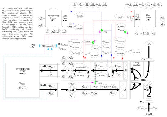
Figure 1.
Operating scheme of the HVAC system (thick solid black lines/arrows: path of air flow; blue lines/arrows: path of cold heat transfer fluid produced by the RS; red lines/arrows: path of hot heat transfer fluid produced by the HP; dashed light blue lines/arrows: parameters controlling the AHU operation; dashed pink lines/arrows: signals controlling the opening of the valves) [51].

Table 1.
Nominal main characteristics of the HVAC system main components.
As shown in Figure 1, the AHU is equipped with three dampers (exhaust air damper DEA, outdoor air damper DOA, and return air damper DRA). All these filters are manufactured by the CLA s.r.l. company (San Giacomo di Teglio, Italy) [54]. Each one is characterized by a frame in galvanised steel (with thickness of 1.0 mm) and airfoil blades in galvanised steel (thickness of 0.5 + 0.5 mm), with distance between blades equal to 100 mm. They are categorized as Class 4 according to EN 1751 Standard [55]. The dimensions of DEA, DOA and DRA, respectively, are the following: 70 × 41 cm2, 70 × 31 cm2 and 40 × 11 cm2. The movement and position of the louvers are controlled by a motor-driven actuator specifically designed for air dampers [56]. The AHU also includes three filters (return air filter FRA, fresh air filter FOA, and supply air filter FSA). All these filters are manufactured by the F.C.R. S.p.A. company (Cinisello Balsamo, Italy) [57], with the following sizes (long side, short side, and thickness, respectively): 59.2 × 28.7 × 4.8 cm3 for FRA, 59.2 × 28.7 × 9.8 cm3 for FOA, and 59.2 × 28.7 × 28.2 cm3 for FSA. FRA and FOA are identical. Filter media is a progressive density synthetic fibre; it is protected by a wire mesh on both sides to ensure the consistency of the pack and the regularity of the pleat (frame is in galvanised steel, while electro-galvanised steel wire mesh protections are used). Both filters are classified as ISO Coarse class 50% according to ISO 16890 [58]. The fresh air filter presents a nominal airflow rate of 2300 m3/h across a 0.4 m2 filtering area, with a filter weight of 1.8 kg and a pressure drop of 70 Pa. The return air filter is characterized by a nominal airflow rate of 1650 m3/h over a 0.3 m2 filtering area, with a filter weight of 1.1 kg and a pressure drop of 70 Pa. FSA is a 3 V rigid bag filter with injection-moulded plastic (polystyrene) frame; its filtering medium is a water repellent fiberglass paper. It is classified as ePM1 85% according to ISO 16890 [58] with a nominal pressure drop of 110 Pa (at a nominal airflow rate of 1700 m3/h).
The HVAC system described in Figure 1 is managed through a specific control logic, implemented and executed in the LabVIEW environment (version 2019 SP1) [59]. End-users have the ability to manually adjust and set the following parameters:
- set-points of indoor air temperature TSP,Room and relative humidity RHSP,Room to be reached in the test room;
- deadbands associated with TSP,Room and RHSP,Room, that are named DBT and DBRH, respectively;
- return air fan and the supply air fan speed (i.e., OLRAF and OLSAF, respectively) in the range between 0% and 100% (those parameters are kept constant throughout all the tests considered in this study);
- opening percentages of the return air damper (OPDRA), the outside air damper (OPDOA), and the exhaust air damper (OPDEA) in the range between 0% and 100%, where 0% indicates that the damper is completely closed (those parameters are kept constant throughout all the tests considered in this work);
- activation/deactivation of the heat-recovery system that is determined by adjusting the opening percentage (between 0% and 100%) of the heat-recovery system damper OPDHRS (heat recovery system is inactive throughout all the tests considered in this research).
As the parameters mentioned above are defined, the operation mode of the HVAC system components (post-heating coil, cooling coil, humidifier, heat pump, and refrigerating system) is determined, regardless to the season, according to the control logics reported in Table 2 (the control logic of the pre-heating coil is omitted from the table as it is deliberately set to the off-mode during all the tests carried out in this study; thus, the demand for heating was only met by the operation of the post-heating coil). In particular, the Heat Pump (HP) is activated only when the temperature of the heat transfer fluid (THT) inside the hot tank (HT) is lower than the desired set-point temperature (THT,set-point) decreased by a specified deadband temperature (DBT,HT); then it remains activated until the temperature of the heat transfer fluid becomes equal to THT,set-point + DBT,HT. The heat transfer fluid is circulated by the pump PHP, which connects the HT and the PostHC/PreHC coils (only when one of the PostHC or PreHC coil valve is open). Regarding the Refrigerating System (RS), it is activated only when the temperature of the heat transfer fluid inside the cold tank (CT) exceeds the desired set-point temperature (TCT,set-point) increased by the specified deadband temperature (DBT,CT); then, it remains activated until the heat transfer fluid temperature becomes equal to TCT,set-point − DBT,CT. The pump PRS circulates the fluid between the CT and the cooling coil (CC) only when the CC valve is open. The heat transfer fluid is a mixture of water and ethylene glycol (about 6% by volume). PID (proportional-integral-derivative) controllers autonomously adjust the valve opening percentages for the post-heating coil (OPV_PostHC), cooling coil (OPV_CC), and humidifier (OPV_HUM). These adjustments ensure that the return air temperature (TRA) remains within the specified upper bound UDBT (UDBT = TSP,Room + DBT) and the lower bound LDBT (LDBT = TSP,Room − DBT) of the deadband of the return air temperature set-point (TSP,Room), while the actual return air relative humidity (RHRA) stays within the upper bound UDBRH (UDBRH = RHSP,Room + DBRH) and the lower bound LDBRH (LDBRH = RHSP,Room − DBRH) of the deadband of the return air relative humidity set-point (RHSP,Room).
Table 2.
Conditions for activating/deactivating the AHU components.
However, the user can override the control signals in order to customize the system operation and, therefore, artificially introduce specific faults (and corresponding intensities) related to specific components of the experimental set-up.
Sensors and Measurement Uncertainty
The HVAC system is fully equipped with a range of sensors that monitor, measure, record, and control crucial operating parameters that are acquired using a management system developed in the LabView environment [59]. Table 3 reports both the measuring range and the accuracy of each sensor. It is important to note that all AHU’s electrical components operate on three-phase power, except the return air fan (RAF) requiring single-phase power. Air temperature TRoom and air relative humidity RHRoom inside the integrated test room are measured in the center of the floor at a height of about 60 cm above the ground. The spatial uniformity of indoor thermo-hygrometric conditions cannot be verified and controlled in this experimental set-up because the corresponding parameters are measured at individual points (as in the case of almost all real-world applications).
Table 3.
Main characteristics of the sensors.
Electric power consumption of the supply air fan (EPSAF), the return air fan (EPRAF), the heat pump (EPHP), the heat pump circulating pump (EPPHP), the refrigerating system (EPRS), the refrigerating system circulating pump (EPPRS), as well as the humidifier (EPHUM) are calculated through the following equations according to the measured values of voltage and current intensity:
where cosφSAF, cosφRAF, cosφHP, cosφPHP, cosφRS, cosφPRS, and cosφHUM are the power factors of the SAF, the RAF, the HP, the PHP, the RS, the PRS, and the HUM, respectively. The following values recommended by the manufacturers have been presumed for the power factors: cosφSAF = 0.95, cosφRAF = 0.95, cosφHP = 0.95, cosφPHP = 0.95, cosφRS = 0.95, cosφPRS = 0.95, and cosφHUM = 0.95.
The absolute measurement errors δ (EPSAF), δ (EPRAF), δ (EPHP), δ (EPPHP), δ (EPRS), δ (EPPRS), and δ (EPHUM) related to the assessment of the electric power consumption of the supply air fan (Equation (1)), the return air fan (Equation (2)), the heat pump (Equation (3)), the circulating pump connected to the heat pump (Equation (4)), the refrigerating system (Equation (5)), the circulating pump connected to the refrigerating system (Equation (6)), and also the humidifier (Equation (7)), respectively, are calculated based on the single-sample uncertainty analysis [66] by using below equations:
where δ (X) in the above formulas denotes the uncertainty of variable X, as listed in Table 3, related to the measured current and voltage values of the SAF, the RAF, the HP, the PHP, the RS, the PRS, and the HUM.
3. Design of Experiments
The AHU serving the test room of the SENS i-Lab has been operated under faulty and fault-free conditions. In particular, 11 experimental tests were carried out during summer and winter season under normal condition (N), namely SN1, SN2, SN3, SN4, SN5, SN6, WN1, WN2, WN3, WN4, and WN5, where the tests SN1–SN6 were performed during the summer (S) 2022, while the other tests WN1–WN5 were conducted during the winter (W) across the years 2022/23. Regarding faulty tests, 14 experiments were performed, namely SF1, SF2, SF3, SF4, SF5, SF6, SF7, WF1, WF2, WF3, WF4, WF5, WF6, and WF7, where the tests SF1–SF7 were carried out during the summer (S) 2022, while the other tests WF1–WF7 were completed during the winter (W) 2023.
Table 4 reports the operating conditions associated to the fault-free experiments, while Table 5 reports the operating conditions of the faulty ones (the cells highlighted with a yellow background report the settings imposed to artificially emulate the malfunctioning of the system components). The set-point values of indoor air temperature and relative humidity inside the test room have been defined according to typical indoor conditions desired in Italian buildings during winter and summer.
Table 4.
Operating conditions of the fault-free experiments.
Table 5.
Operating conditions of the faulty experiments.
It should be noted that a single fault type/severity was investigated during each faulty test by manually setting the position of the return air damper, the outdoor air damper, and the exhaust air damper to a constant value (i.e., 0% or 100%) to emulate a damper stuck. On the other hand, the outdoor air filter, the supply air filter, and the return air filter faults were manually obstructed to emulate a filter clogging at 50% by covering the filters with a single-wall corrugated cardboard, where the covered area represented the fault severity.
According to the test IDs reported in Table 5, the following seven fault types/severities were implemented during the operational hours of the system (from 9:00 a.m. to 6:00 p.m.), specifically:
- fault 1: return air damper kept always closed (stuck at 0%) during the faulty tests SF1 and WF1 (i.e., OPDRA = 0%);
- fault 2: fresh air damper kept always closed (stuck at 0%) during the faulty tests SF2 and WF2 (i.e., OPDOA = 0%);
- fault 3: fresh air damper kept always open (stuck at 100%) during the faulty tests SF3 and WF3 (i.e., OPDOA = 100%);
- fault 4: exhaust air damper kept always closed (stuck at 0%) during the faulty tests SF4 and WF4 (i.e., OPDEA = 0%);
- fault 5: fresh air filter partially clogged at 50% during the faulty tests SF5 and WF5 (i.e., OPFOA = 0%);
- fault 6: supply air filter partially clogged at 50% during the faulty tests SF6 and WF6 (i.e., OPFSA = 0%);
- fault 7: return air filter partially clogged at 50% during the faulty tests SF7 and WF7 (i.e., OPFRA = 0%).
4. Comparison of Boundary Conditions Between Fault-Free and Faulty Tests
The fault-free tests (SN1–SN6 and WN1–WN5) were assumed as reference baselines to be compared with the faulty tests (SF1–SF7 and WF1–WF7) in order to assess the impacts associated to a specific faulty condition.
To this purpose, the initial indoor conditions for all the tests (fault-free and faulty) conducted in summer are approximately the same and equal to about 28 °C and 60% for TRA and RHRA, respectively; similarly, the initial indoor conditions are consistent for both faulty and normal tests during winter, with starting values of about 18 °C for the room air temperature (TRA) and 60% for the relative humidity of the room air (RHRA).
Furthermore, for each faulty test there is a corresponding normal test similar in terms of outdoor air temperature (TOA) and outdoor air relative humidity (RHOA) according to the following metrics evaluated for each pair of tests:
where EXPOA,Normal,i and EXPOA,Faulty,i are, respectively, the experimental values of TOA or RHOA at time step i for normal and faulty tests, represents the average difference, is the average absolute difference, N is the number of experimental data points, and RMSD is the root mean square difference.
εi = EXPOA,Normal,i − EXPOA,Faulty,i
Table 6 reports the obtained values of , and RMSD for each pair of normal and faulty tests. In the table, the worst values of , and RMSD are reported in red, while the best values of , and RMSD are reported in green.
Table 6.
Comparison between normal and faulty tests in terms of outside air temperature TOA and outside air relative humidity RHOA.
Table 6 shows that the highest absolute values of , and RMSD are, respectively, equal to 1.57 °C, 1.59 °C, 1.32 °C for TOA and −8.20%, 8.87%, 8.41% for RHOA. The data provided in this table highlights that the values of are always less than 1.6 °C in terms of TOA and lower than 10.0% in terms of RHOA.
Further information regarding the boundary conditions comparison between normal and faulty tests can be found in [49,50]. According to the process suggested in [32], it is possible to conclude that the identified pairs of fault-free and faulty tests can be considered as subjected to boundary conditions enough similar between each other to enable a robust comparison. For the sake of completeness, the following bullet points report all the normal-faulty pairs of tests considered for conducting the impact analysis:
- the normal test SN3 can be compared against the faulty test SF1;
- the normal test SN1 can be compared against the faulty test SF2;
- the normal test SN5 can be compared against the faulty test SF3;
- the normal test SN4 can be compared against the faulty test SF4;
- the normal test SN2 can be compared against the faulty test SF5;
- the normal test SN5 can be compared against the faulty test SF6;
- the normal test SN6 can be compared against the faulty test SF7;
- the normal test WN1 can be compared against the faulty tests WF1 and WF3;
- the normal test WN2 can be compared against the faulty tests WF5 and WF7;
- the normal test WN3 can be compared against the faulty test WF2;
- the normal test WN4 can be compared against the faulty test WF6;
- the normal test WN5 can be compared against the faulty test WF4.
5. Methods and Results
This section reports the results of the comparison between the fault-free and faulty tests to assess the fault impacts on the operation of HVAC system components. Section 5.1 considers the main effects that the analysed faults have on indoor thermo-hygrometric conditions, while Section 5.2 discusses the impact on electrical power and energy consumption. In Section 5.3, the effects of faults on the key operating parameters are analysed. The analyses have been performed by means of well-defined single-criteria key performance indicators that well fit with the purpose of quantify the impact of specific faulty conditions on AHU operation; this will make it possible to rank faults according to their impact under different operating conditions based on a fault scenario analysis, as well as evaluate a maintenance action prioritization scheme considering how the impact of a fault changes during system operation.
5.1. Effects of Faults on Indoor Thermo-Hygrometric Conditions
This section provides a complete analysis of the effects of the studied faults on indoor air temperature and relative humidity. Specifically, for each pair of corresponding normal and faulty experiments, Table 7 shows the values of both the percentage of time during which indoor air temperature is kept within the defined deadbands (TCT) as well as percentage of time during which indoor air relative humidity is kept within the defined deadbands (HCT). Additionally, this table reports the relevance of deviations from desired indoor air temperatures and the relevance of deviations from desired indoor air relative humidity values , which quantify the intensity of fault impacts on indoor thermo-hygrometric conditions, respectively. These four metrics are calculated by using the following formulas:
where:
Table 7.
Percentage of time during which indoor air temperature/relative humidity is kept within the defined deadbands and relevance of deviations from desired indoor air temperature/relative humidity values during fault-free and faulty tests.
- Nin,DBT and Nin,DBRH represent the number of experimental data points corresponding to operating conditions where TRA and RHRA, respectively, fall between their corresponding deadbands;
- ΔTout,DBT,i represents the deviation between the actual temperature of return air (TRA,i) at a specific time step i and the corresponding upper deadband UDBT or lower deadband LDBT;
- ΔRHout,DBRH,i is the difference between the actual relative humidity of return air (RHRA,i) at a specific time step i and the corresponding upper deadband UDBRH or lower deadband LDBRH;
- N represents the total number of data points collected for each test. Considering a 1 s monitoring interval and an operational schedule from 9:00 am to 6:00 pm; this translates to 32,400 experimental data points;
- Nout,DBT and Nout,DBRH represent the number of experimental data points corresponding to operating conditions where TRA and RHRA, respectively, fall outside their corresponding deadband limits (either upper or lower).
It should be mentioned that percentage of time during which indoor air temperature/relative humidity are kept within the defined deadbands observed in normal tests falls below 100% due to two primary factors: Firstly, the initial values of the return air temperature and relative humidity deviate considerably from the predetermined target values, necessitating a substantial duration to converge towards the desired setpoints from the beginning of the tests. Secondly, during the start-up phases, the AHU operates under transient conditions as it endeavours to attain steady-state performance.
Figure 2 shows the following percentage difference (%DCT) between each normal and corresponding faulty test:
where CTNormal and CTFaulty are the test durations during which indoor air temperature or relative humidity is kept within the defined deadbands during normal and faulty tests, respectively. A negative value for %DCT indicates the system’s inability to maintain the desired indoor air temperature/relative humidity values under faulty conditions.
%DCT = CTFaulty − CTNormal
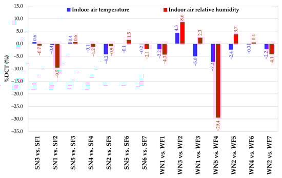
Figure 2.
Values of %DCT as a function of the normal/faulty tests under comparison.
- the fault 1 (i.e., return air damper always closed) had minor effects on indoor thermo-hygrometric conditions in either summer or winter tests (between 0.6% and −4.3%, respectively);
- the fault 2 (i.e., fresh air damper kept always closed) resulted in a 9.5% decrease in HCT during summer, dropping from 94.2% during the normal test down to 84.7% during the faulty test; however, TCT during summer was minimally impacted. In contrast, during winter the fault 2 (test WF2) increased HCT in comparison with the normal winter test (WN3), with values of 97.7% and 89.2%, respectively. These results could be related to the absence of fresh air, allowing smaller fluctuations in terms of indoor air humidity as well as more stable hygrometric conditions;
- the fault 3 (i.e., fresh air damper kept always open) impacted TCT/HCT of less than 1% during summer, while it determined a 5% decrease in TCT during winter;
- the fault 4 (i.e., exhaust air damper kept always closed) had minor effects on TCT/HCT during summer test, while it caused a reduction in TCT and HCT of 7.2% and 29.4%, respectively;
- the fault 5 (i.e., fresh air filter clogged at 50%) did not affect TCT and HCT significantly, neither in summer nor winter. The highest reduction in terms of TCT/HCT caused by the fault F5 pertains to the test SF5, when TCT was reduced by about 4.2%;
- the fault 6 (i.e., supply air filter clogged at 50%) did not affect TCT/HCT during both summer and winter;
- the fault 7 (i.e., return air filter clogged at 50%) resulted in 4.1% HCT reduction in the faulty test WF7 compared to the normal test WN2, while HCT/TCT during summer tests were negligible.
The relevance of deviations from desired indoor air temperature for all the faults is equal or less than 0.52 °C. Similarly, the relevance of deviations from desired indoor air relative humidity values for all the faults is equal or less than 2.9%, as indicated in Table 7.
In summary, since OPDRA, OPDOA, and OPDEA remain constant across all normal and faulty tests, the AHU can guarantee the desired values of indoor air temperature and relative humidity by adjusting OPV_PostHC, OPV_CC, and OPV_HUM, as well as activating HP/RS/HUM in order to compensate for the effects of the implemented faults. In this sense, fault impact assessment requires a comprehensive analysis that considers not only indoor thermo-hygrometric conditions, but also deviations in terms of electric consumption as well as operation time of each AHU component.
5.2. Effects of Faults on Electrical Demand and Operation Time
This section provides a complete analysis of the impacts of the considered faults on electrical power consumption, electrical energy demand and operation time of AHU components. Specifically, for each pair of corresponding normal and faulty experiments, Table 8 and Table 9 present the arithmetic mean (μ) and the standard deviation (σ) of electric power consumption (EP), and their relative percentage difference (%EP), which is calculated as follows:
where EPNormal and EPFaulty are, respectively, the arithmetic mean μ or the standard deviation σ of the electric power consumption of AHU components operated in normal and faulty conditions. Table 8 refers to summer tests, while Table 9 correspond to winter experiments. In Table 8 and Table 9, cells reporting the values of %EP have been colour coded based on the legend provided, reflecting the significance of the values derived from Equation (24).
Table 8.
Electric power consumption (EP) of faulty and normal summer tests as well as corresponding percentage difference for each system component calculated via the parameter %EP (Equation (24)).
Table 9.
Electric power consumption (EP) of faulty and normal winter tests as well as corresponding percentage difference for each system component calculated via the parameter %EP (Equation (24)).
Specifically, cells displaying the highest %EP values are highlighted in red to pinpoint the most significant differences between faulty and normal tests. The mean electrical power consumption of the recirculating pumps of the RS and the HP are not included in Table 8 and Table 9, as the electrical power consumption of these auxiliary systems remain almost constant even after fault induction.
The assessment of measurement uncertainties associated to electric power consumption of the supply air fan, return air fan, refrigerating system, and heat pump was conducted by using Equations (8)–(14). Based on the experimental data, the highest absolute errors for EPSAF, EPRAF, EPRS, and EPHP are 24.64 W, 4.04 W, 103.21 W, and 105.54 W, corresponding to maximum relative errors of 6.98%, 5.32%, 10.09%, and 11.96%, respectively.
As can be seen in Table 8, the difference between faulty tests and their corresponding fault-free tests in terms of average power consumption is between −10% and 10% for all the reported AHU components of every fault during summer. Similar data (between −10% and 10%) can be recognized with respect to the standard deviation values of electric power consumption, except for the humidifier (in the cases of faults 1 and 4) and the heat pump in the case of fault 3. For what is concerned the winter tests (Table 9), the average power consumption variation between normal and faulty tests is between −10% and 10% for all the assessed AHU components, except from the RS mean power consumption differences caused by the faults F2 and F5 (10.89% and −10.04%, respectively), the HP mean power consumption difference caused by the fault F7 (−10.34%), and the HUM mean power consumption difference associated to the fault F3 (−100%). The percentage difference of standard deviation of AHU components’ electric power consumption between faulty and normal are higher than 10% or lower than −10% in the following cases: (i) the SAF in the cases of the faults F2 and F5; (ii) the RAF during the winter faulty tests WF1, WF2, and WF3; (iii) the RS in the case of the faults F2 and F4; (iv) the HP in the case of the faults F1, F2, and F3; and (v) the HUM in the case of the fault F3.
Table 10 and Table 11 report the electrical energy consumption (EE) of (1) the supply air fan (EESAF), (2) the return air fan (EERAF), (3) the refrigerating system (EERS), (4) the circulating pump connected to the refrigerating system (EEPRS), (5) the heat pump (EEHP), (6) the circulating pump connected to the heat pump (EEPHP), and (7) the humidifier during fault-free and corresponding faulty experiments; these tables include also the percentage difference between faulty and fault-free tests in terms of electric energy consumption (%EE), calculated as follows:
where EENormal and EEFaulty are, respectively, the electric energy consumption of AHU components during normal and corresponding faulty tests.
Table 10.
Electric energy consumption (EE) of faulty and normal summer tests as well as corresponding percentage difference for each system component calculated via the parameter %EE (Equation (25)).
Table 11.
Electric energy consumption (EE) of faulty and normal winter tests as well as corresponding percentage difference for each system component calculated via the parameter %EE (Equation (25)).
Each cell of the rows reporting the parameter %EE in Table 10 and Table 11 is coloured according to the magnitude of the difference itself. Specifically, if the percentage difference falls within the range ±10%, the cell is filled in yellow; alternatively, if the absolute differences are greater than 20%, the cell is filled in red; otherwise, for intermediate cases the cells are coloured in orange.
Figure 3 shows the percentage differences between normal and faulty tests in terms of electrical energy demand (calculated via the parameter %EE (Equation (25)) during summer (a) and winter (b). The percentage difference (%EE) for individual AHU components is reported only when it is greater than or equal to 10%, while the total energy consumption is reported whatever the value is.
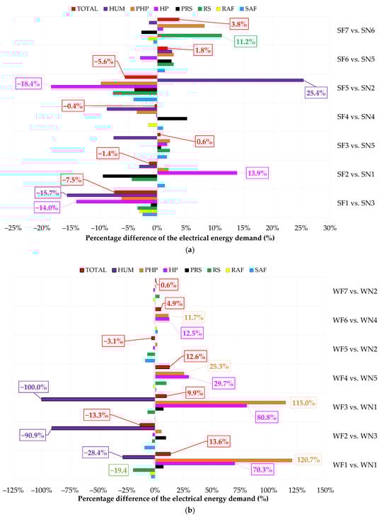
Figure 3.
Percentage difference between normal and faulty tests in terms of electrical energy demand during summer (a) and winter (b) calculated via the parameter %EE defined by Equation (25).
Table 12 and Table 13 report the operation time OT (i.e., the time during which the component was active/used of (1) the supply air fan (OTSAF), (2) the return air fan (OTRAF), (3) the refrigerating system (OTRS), (4) the heat pump (OTHP), (5) the humidifier (OTHUM), (6) the circulating pump connected to the refrigerating system (OTPRS), and (7) the circulating pump connected to the heat pump (OTPHP) during fault-free and corresponding faulty experiments). The percentage difference between faulty and fault-free tests in terms of operating time (%OT) is calculated as follows and also included in Table 12 and Table 13:
where OTNormal and OTFaulty are, respectively, the operating time of AHU components during fault-free tests and corresponding faulty tests. Each cell of the rows reporting the parameter %OT in Table 12 and Table 13 is coloured according to the magnitude of the parameter itself (as indicated in the legend).
Table 12.
Operating time (OT) of faulty and normal summer tests as well as corresponding percentage difference for each system component calculated via the parameter %OT (Equation (26)).
Table 13.
Operating time (OT) of faulty and normal winter tests as well as corresponding percentage difference for each system component calculated via the parameter %OT (Equation (26)).
Figure 4a,b present the percentage time differences between normal and faulty tests in terms of operation time (calculated via the parameter %OT defined by Equation (26)) during summer (a) and winter (b); the values for individual components are highlighted only when their absolute values are greater than or equal to 10%.
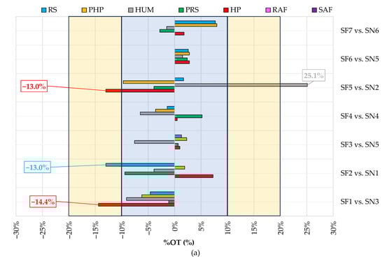
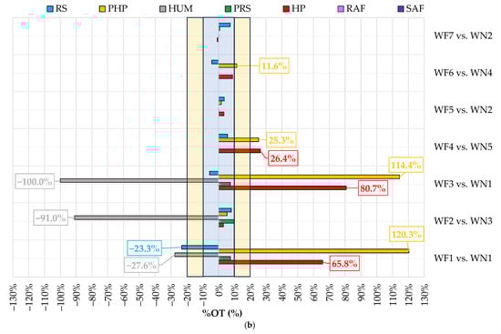
Figure 4.
Percentage difference between normal and faulty tests in terms of operational time during summer (a) and winter (b) calculated via the parameter %OT defined by Equation (26).
Based on Table 10, Table 11, Table 12 and Table 13 as well as Figure 3 and Figure 4, the following results regarding the effects of considered faults on AHU components’ electric energy consumption can be derived:
- the fault 1 (i.e., return air damper stuck at 0%) had a considerable impact on HP electrical energy consumption, increasing it by about 70% during winter and reducing it by about 14% in summer with respect to normal conditions. In contrast, RS electric energy demand showed only minor variations during summer, with a difference of about 3% between normal and faulty tests. During winter, the fault 1 resulted in a decrease of about 19% of RS electrical consumption. Additionally, this fault resulted in reduced electrical consumption demand of the humidifier by about 15% in summer and about 28% during winter. Total electric demand associated to the fault 1 increased by about 14% during winter because only cold fresh air is used, while it reduced during summer by about 7% because the utilization of hot outdoor air is more than counterbalanced by the significantly decreased supply airflow rate elaborated by the AHU;
- the fault 2 (characterized by the fresh air damper being stuck at 0%) led to a reduction in total electrical energy consumption of approximately 13% with respect to the corresponding normal test; this was largely due to a significant decrease (more than 90%) in humidifier electrical energy consumption, while the electrical energy consumption of other AHU components remained largely unchanged. It is important to note that while this fault resulted in lower total energy consumption during winter because of the fact that only return air is used, it enhanced percentage of time during which indoor air temperature and relative humidity are kept within the defined deadbands. During summer, the changes included a 14% increase in HP electric energy consumption and a 10% decrease in PRS electric demand, determining a negligible reduction (about 1%) in terms of total electrical consumption; the slightly reduced electric demand is counterbalanced by a decrease of about 9% in terms of percentage of time during which indoor air relative humidity is kept within the defined deadbands during the faulty test SF2 compared to the normal test SN1. It should be underlined that the exclusive use of return air without any fresh air intake likely has negative implications for IAQ, even if IAQ was not directly assessed in this study;
- the fault 3 (i.e., fresh air damper stuck at 100%) led to the most significant rise in HP electric energy consumption observed during the winter tests among all the investigates faulty scenarios. Indeed, during the winter faulty test, it resulted in an 81% increase in total HP electric demand compared to the normal one because of the fact that larger flowrate of fresh air is used. In addition, it is also noteworthy that the humidifier remained completely inactive during the test WF3, as the increased operation of the HP had a reduced demand for humidification as a counter effect; on the other hand, no significant effects have been recognized during the summer test;
- the fault 4 (i.e., exhaust air damper stuck at 0%) during summer determined the occurrence of minor differences in terms of electric energy consumption between the faulty and normal scenarios. However, in the winter tests, the HP electric demand increased by about 30% compared to the fault-free test, with a total electrical consumption increased by about 13%. Notably, the winter faulty test WF4 also experienced the most significant reductions in both percentage of time during which indoor air temperature and relative humidity are kept within the defined deadbands, with decreases of approximately 7% and 29%, respectively;
- the fault 5 (i.e., fresh air filter clogged at 50%) did not result in significant variations (about 3%) in terms of total electric energy consumption of AHU components during the faulty winter test compared to the normal one. However, a reduced outdoor air volumetric flowrate led to an 8% decrease in RS energy consumption and, consequently, an approximate 18% reduction in HP electrical demand during the summer faulty test compared to the summer normal experiment; this reduction caused a 25% increase in humidifier electrical energy consumption (as the demand for humidification increased taking into account the decrease in RS energy consumption); as a result, the fault 5 allowed a reduction of about 5% in total electric demand during summer (this effect is counterbalanced by a reduced percentage of time during which indoor air temperature is kept within the defined deadbands by about 4%);
- the fault 6 (corresponding to the supply air filter clogged at 50%) resulted in a 12% increase in heat pump electrical energy consumption during the winter faulty test WF6 compared to the winter normal test WN4. This increase can be attributed to the lower supply air flow rate in the faulty test, which necessitated a higher air temperature to meet the indoor setpoint temperature. The total electric demand increased by about 5% under winter conditions. During the summer tests, the effect of the reduced supply air volumetric flow rate was counterbalanced by an increase in cooling energy demand, which led to a 3% increase in RS energy consumption to meet indoor thermo-hygrometric requirements. Additionally, the increased operation of the refrigerating system also had a dehumidifying effect, resulting in about a 3% rise in humidifier electrical energy consumption during the summer faulty test SF6 respect to SN5; the overall electrical demand slightly increased by about 2% during summer;
- the fault 7 (i.e., return air filter clogged at 50%) resulted in a reduced return air flowrate, which consequently increases the fresh air flowrate. Specifically, RS energy consumption increased during both summer (by about 11%) and winter (by about 4%); the effects on the other AHU components were negligible.
Deshmukh et al. [41] reported that an outdoor air damper stuck in the fully open position results in energy waste, with an increment of about 18% of energy expense during a particular winter month. Additionally, Lu et al. [67] underlined that an outdoor air damper stuck in the fully open position significantly increases energy consumption by about 14%, whereas a decrease in energy demand of nearly 26% occurs when the outdoor air damper stuck is stuck in the fully closed position. The outcomes of both scientific researches [41,67] are consistent with the experimental findings of this work. Wang and Hong [45] investigated a list of maintenance issues (including outdoor air damper leakage, outdoor air damper stuck at fully open position, and dirty filters) via field surveys and simulation models. According to [45], filters clogging can affect electric energy demands of fans (together with pressure drops and airflow rates); this result is aligned with the outcomes of this study where an impact in terms of fan energy demand caused by filters faults is also recognized.
To summarize, this section discussed the impact of faults on indoor air temperature and relative humidity, together with electrical demands. Considering the negligible variations of average power consumption of almost all AHU components between normal tests and their associated faulty tests, it can be concluded that faults have had higher effects on operation time and total energy consumption of AHU components rather than mean power consumption (Table 10, Table 11, Table 12 and Table 13). It is also evident that, with the exceptions of the faulty test WF1 (where the return air damper was kept always fully closed) and the faulty test WF4 (where the exhaust air damper was kept always fully closed), the influence of all other faults was generally minimal, affecting both percentage of time during which indoor air temperature/relative humidity are kept within the defined deadbands and total electric energy consumption by no more than 10%. Notably, during winter the fault F1 resulted in a 14% increase of total electric energy consumption but did not significantly affect indoor thermo-hygrometric conditions. Conversely, during winter the fault F4 determined a substantial reduction in terms of percentage of time during which indoor air relative humidity is kept within the defined deadbands by about 29%, coupled with about 13% increase in total electrical demand. In terms of operation time of AHU components, it can be observed (from Table 12 and Table 13 as well as Figure 4) that in most of the faulty experiments the percentage differences between normal and faulty tests are in the range of ±10% mainly during summer tests. Notably, the largest percentage differences in operation times are observed during the winter tests, particularly for the heat pump (and its circulating pump) as well as the humidifier; in particular, it changes between a minimum of -100% obtained for the HUM during the faulty winter test WF3 up to a maximum of 120% obtained for the PHP during the faulty winter test WF1, highlighting significant deviations from typical performance under normal conditions.
5.3. Effects of Faults on Key Operating Parameters
Assessing the impact of typical faults on AHU key operating parameters is crucial for the development of data-driven Fault Detection and Diagnostics (FDD) tools. The knowledge of such patterns represents an essential feature for the definition of robust FDD systems. In this perspective, Figure 5, Figure 6 and Figure 7 summarize the impact that each considered fault had on some of the most relevant operating parameters, reporting their arithmetic mean (μ) and standard deviation (σ). Specifically, 14 parameters are considered in this analysis, pertaining to air temperature, fluid temperature, and air relative humidity. The air temperature related parameters include TRA, TMA, TA,out,CC, TA,out,PostHC, and TSA (shown in Figure 5); the fluid temperature related parameters, such as TF,out,CC, TF,in,CC, TF,out,PostHC, and TF,in,PostHC, are reported in Figure 6, while the air relative humidity related parameters, including RHRA, RHMA, RHA,out,CC, RHA,out,PostHC, and RHSA, are indicated in Figure 7.
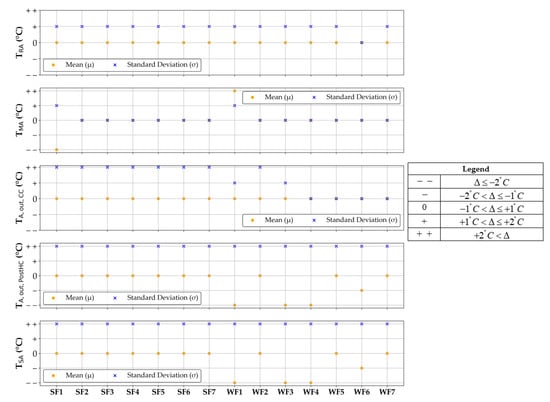
Figure 5.
Fault symptom relevance in terms of air temperature.
Figure 6.
Fault symptom relevance in terms of fluid temperature.
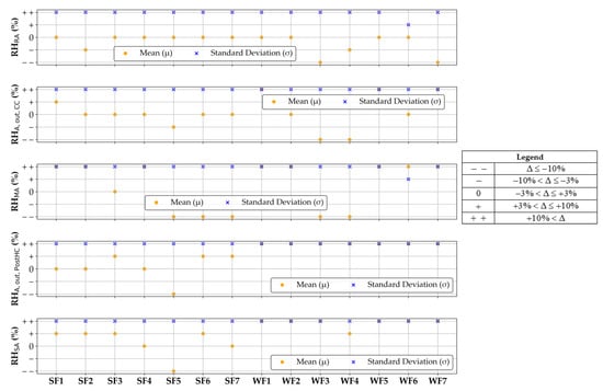
Figure 7.
Fault symptom relevance in terms of relative humidity.
The effects of each fault on the considered key operating parameters are here discussed in detail by using the following qualitative scale to improve the readability of the obtained results:
- “0” means that the fault does not lead to significant changes;
- “+” means that the fault leads to minor positive changes;
- “+ +” means that the fault leads to significant positive changes;
- “-” means that the fault leads to minor negative changes;
- “- -” means that the fault leads to significant negative changes.
In accordance with this scale, Figure 5, Figure 6 and Figure 7 report the symptoms’ relevance associated with the considered faults based on the values taken by the parameter ∆:
where XFaulty and XNormal denote the arithmetic mean (μ) or the standard deviation (σ) calculated from the measurements obtained under faulty and normal conditions, respectively.
Δ = XFaulty − XNormal
Considering Figure 5, Figure 6 and Figure 7, the following results regarding key operating parameters can be derived:
- the fault 1 (i.e., return air damper stuck at 0%) led to a noticeable deviation of arithmetic means associated to TMA, TA,out,PostHC, TSA, TF,out,PostHC, TF,in,PostHC, RHMA, RHA,out,CC, RHA,out,PostHC, and RHSA during the winter faulty test WF1 with respect to the normal winter test WN1; with reference to the same season, the impact of the same fault F1 is also relevant in the cases of the standard deviations of TA,out,PostHC, TSA, TF,out,PostHC, TF,in,PostHC, RHRA, RHMA, RHA,out,CC, RHA,out,PostHC, and RHSA. The fault F1 relevantly changes the arithmetic means of TMA and RHMA as well as the standard deviations of TA,out,CC, TA,out,PostHC, TSA, TF,out,PostHC, RHRA, RHMA, RHA,out,CC, RHA,out,PostHC, and RHSA when comparing the faulty summer test SF1 and the normal summer test SN3;
- the fault 2 (i.e., fresh air damper stuck at 0%) had a significant impact on the arithmetic means of RHMA, RHA,out,PostHC, and RHSA as well as the standard deviations of TA,out,CC, TA,out,PostHC, TSA, TF,out,PostHC, TF,in,PostHC, RHRA, RHMA, RHA,out,CC, RHA,out,PostHC, and RHSA during the faulty winter test WF2 compared to the normal winter test WN3. The arithmetic means of RHMA together with the standard deviations of TA,out,CC, TA,out,PostHC, TSA, TF,out,PostHC, TF,in,PostHC, RHRA, RHMA, RHA,out,CC, RHA,out,PostHC, and RHSA during the summer faulty test SF2 with respect to the corresponding normal summer test. The effects on air relative humidity are mainly due to a relevant reduction in humidifier operation time (by about −91% as indicated in Figure 4b);
- the fault 3 (i.e., fresh air damper stuck at 100%) caused a relevant change in the standard deviations of TA,out,CC, TA,out,PostHC, TSA, TF,out,PostHC, TF,in,PostHC RHRA, RHMA, RHA,out,CC, RHA,out,PostHC, and RHSA during summer (while the arithmetic means were not significantly affected). During winter, both the arithmetic means and standard deviations of TA,out,PostHC, TSA, TF,out,PostHC, TF,in,PostHC, RHRA, RHMA, RHA,out,CC, RHA,out,PostHC, and RHSA were considerably impacted. These results are also a consequence of longer operation time of HP and reduced HUM operation time during the winter faulty test in comparison to the winter normal test (respectively, by about 80% and −100%, as reported in Figure 4b);
- the fault 4 (i.e., exhaust air damper stuck at 0%) determined a relevant decrease in arithmetic means associated to TA,out,PostHC, TSA, TF,out,PostHC, TF,in,PostHC, RHMA, and RHA,out,CC, together with a significant increase of RHA,out,PostHC during the winter faulty test WF4 compared to the winter normal test WN5. It should be noted that, despite a slight variation of RHRA arithmetic mean (as it indicated in Figure 7) with reference to winter operation, the percentage of time during which indoor air relative humidity is kept within the defined deadbands during the faulty winter test decreased by about 29% as displayed in Figure 2; this is because, despite the fact that RHRA was out of the defined deadbands, its values were close to the upper bound of the deadband UDBRH (55% in all conducted tests). On the other hand, the observed variations of arithmetic means of all the key operating parameters were negligible during summer, except in the case of RHMA; during the summer, the standard deviations of TA,out,PostHC, TSA, TF,out,PostHC, TF,in,PostHC, RHRA, RHMA, RHA,out,CC, RHA,out,PostHC, and RHSA considerably changed;
- the fault 5 (i.e., fresh air filter clogged at 50%) resulted in relevant variations of arithmetic means of RHMA, RHA,out,PostHC, and RHSA during summer and RHMA, RHA,out,CC, RHA,out,PostHC, and RHSA during winter;
- the fault 6 (corresponding to the supply air filter clogged at 50%) lead to remarkable changes in the arithmetic means of the following key operating parameters during winter: RHMA, RHA,out,PostHC, and RHSA; during summer, the arithmetic mean of RHMA is mainly affected;
- the fault 7 (i.e., return air filter clogged at 50%) significantly impacted on the arithmetic means of RHRA, RHMA, RHA,out,CC, RHA,out,PostHC, and RHSA during winter. During summer, the arithmetic mean of RHMA is strongly impacted. This was mainly due to lower share of return air with higher relative humidity than fresh air in supply air.
6. Conclusions
This study focused on evaluating the effects of seven typical filter/damper faults on a typical single-duct dual-fan constant air volume air-handling unit (AHU) based on filed experimental data. The performed analysis aimed to determine the impacts of these faults on various factors, including indoor thermo-hygrometric conditions, electrical power and energy consumption, operational times of AHU components, as well as patterns of key operating parameters. This comprehensive analysis provided insights into how different faults influence the performance and efficiency of the AHU system, thereby affecting indoor environmental quality and energy usage. The evaluation was carried out by comparing experimental data from fault-free and faulty tests, which took place during summer and winter under Mediterranean climate conditions.
The main goals achieved by this study (addressing several research gaps highlighted in the literature review) can be summarized as follows:
- a reference dataset based on experimental campaigns characterized by high resolution measurements of both normal and faulty operation of a typical existing monitored AHU under different modes and weather/load conditions was developed;
- the impact and symptoms of tested faults on indoor thermo-hygrometric conditions and electric energy consumption were quantitatively assessed under a wide range of boundary conditions. In particular, the experimental results revealed that the fault 4 (exhaust air damper stuck at 0%) during winter was the most detrimental in terms of percentage of time during which indoor air relative humidity is kept within the defined deadbands. However, none of the faults studied had a substantial impact on the percentage of time during which indoor air temperature is maintained within the defined deadbands. It was also observed that the majority of the summer faults (SF1, SF2, SF4, SF5) actually decreased total electrical energy consumption, while the remaining summer faults did not lead to significant variations. On the contrary, winter faults displayed a different pattern, with the tests WF1, WF3, and WF4 resulting in a more than 10% variation of electrical energy demand;
- the experimental dataset and the results of faults impact assessment represent a fundamental source of knowledge for supporting the scientific community in defining and/or validating simulation models and data-driven FDD tools to be applied in AHUs.
A secondary scope of this study was to complement previous fault impact analyses pertaining to typical faults such as temperature/relative humidity sensor’s bias, return/supply fan failure, heating/cooling coils stuck, and humidifier valve stuck [49,50,68]. The experimental datasets will be made publicly available on a data repository well-recognised by researchers, so that designers, researchers, policy makers, and facility managers can benefit from a detailed and wide impact analysis, providing valuable motivations for the implementation of Automated Fault Detection and Diagnostics (AFDD) and improved maintenance strategies in HVAC systems. This comprehensive analysis helps stakeholders understand the diverse effects of faults on system performance, guiding them towards more effective and efficient solutions. These improvements can then lead to better system reliability, enhanced operational efficiency, and reduced maintenance costs, ultimately contributing to optimal HVAC system management.
With reference to the main limitations of this study, it should be indicated that the experiments and related results were derived with reference to a specific AHU scheme with particular components’ technologies and sizes operated under a certain control logic in Mediterranean climatic conditions. Although the AHU studied in this paper is absolutely representative of systems typically in use in many applications, the transferability and scalability of the obtained datasets and results to AHUs different from the one used in this study will need to be investigated more extensively and in more detail in the future.
In terms of future work, this study has the potential to be further expanded. From an experimental point of view, while numerous faults related to secondary HVAC systems have been extensively studied and artificially applied to AHUs as detailed in the literature, other types of faults, such as controller malfunctions or duct leakages, have not yet been thoroughly investigated. Furthermore, the exploration of abrupt faults, gradual faults, faults of varying severities, intermediate climatic conditions, and simultaneous faults represents potential aspects to be further explored in future investigations. These additional tests could provide a more comprehensive understanding of how different types of faults impact AHU performance under various conditions.
Furthermore, as can be interpreted from the result and discussion section, all the assessed faults except for WF1 and WF4 did not show severe influences on both indoor thermo-hygrometric conditions and electric energy consumption. However, they obviously have implications on indoor environmental quality (e.g., CO2 and volatile organic compounds concentrations); this denotes the necessity of new parameters and variables to be assessed and measured in the future tests, especially for the fault 2 (fresh air damper kept always stuck at 0%), the fault 4 (exhaust air damper kept always stuck at 0%), the fault 5 (fresh air filter partially clogged at 50%), the fault 6 (supply air filter partially clogged at 50%), and the fault 7 (return air filter partially clogged at 50%).
The authors will upload the collected experimental data for all the considered faults (including faults evaluated in [49,50]) in a publicly accessible data repository. This will enable AFDD developers, AFDD users, and research organizations to exploit experimental data for institutional and research purposes. Additionally, FDD methods developed in the literature can be tested on this dataset to be qualified in terms of performance and reliability, which has become one of the main concerns in this field.
Author Contributions
Conceptualization, A.R., M.E.Y., R.M., A.H., M.S.P. and A.C.; methodology, A.R., M.E.Y., R.M., A.H., M.S.P. and A.C.; software, A.R., M.E.Y., R.M., A.H., M.S.P. and A.C.; validation, A.R., M.E.Y., R.M., A.H., M.S.P. and A.C.; formal analysis, A.R., M.E.Y., R.M., A.H., M.S.P. and A.C.; investigation, A.R., M.E.Y., R.M., A.H., M.S.P. and A.C.; resources, A.R. and A.C.; data curation, A.R., M.E.Y., R.M., A.H., M.S.P. and A.C.; writing—original draft preparation, A.R., M.E.Y., R.M., A.H., M.S.P. and A.C.; writing—review and editing, A.R., M.E.Y., R.M., A.H., M.S.P. and A.C.; visualization, A.R., M.E.Y., R.M., A.H., M.S.P. and A.C.; supervision, A.R. and A.C.; project administration, A.R. and A.C.; funding acquisition, A.R. and A.C. All authors have read and agreed to the published version of the manuscript.
Funding
This research was funded by the Italian Ministry of University and Research (MUR), grant number E53D23002840006.
Data Availability Statement
Dataset available on request from the authors.
Acknowledgments
This study has been performed in the framework of the PRIN 2022 research project titled “UTMOST FDD: an aUToMated, Open, Scalable and Transparent Fault Detection and Diagnosis process for air-handling units based on a hybrid expert and artificial intelligence approach. From experimental open data to transfer model learning for the enhancement of energy management and indoor environmental quality in buildings” (CUP: E53D23002840006) funded by the Italian Ministry of University and Research (MUR). The work of Marco Savino Piscitelli was carried out within the Ministerial Decree no. 1062/2021 and received funding from the FSE REACT-EU—PON Ricerca e Innovazione 2014–2020.
Conflicts of Interest
The authors declare no conflicts of interest.
Nomenclature
| Symbols | |
| A | Current intensity (A) |
| AFDD | Automated fault detection and diagnosis |
| AHU | Air-handling unit |
| CAV | Constant air volume |
| CC | Cooling coil |
| cosφ | Power factor of the AHU component |
| CT | Cold tank |
| CTNormal | Test duration during which indoor air temperature or relative humidity is kept within the defined deadbands during normal tests (min) |
| CTFaulty | Test duration during which indoor air temperature or relative humidity is kept within the defined deadbands during faulty tests (min) |
| DB | Deadband |
| DEA | Exhaust air damper |
| DOA | Outside air damper |
| DHRS | Damper of the heat recovery system |
| DRA | Return air damper |
| EA | Exhaust air |
| EE | Electric energy consumption (kWh) |
| EP | Electric power consumption (W) |
| EXP | Experimental value |
| FOA | Outside air filter |
| FRA | Return air filter |
| FSA | Supply air filter |
| FDD | Fault detection and diagnosis |
| HCT | Percentage of time during which indoor air relative humidity is kept within the defined deadbands (%) |
| HP | Heat pump |
| HRS | Static cross-flow heat recovery system |
| HT | Hot tank |
| HUM | Humidifier |
| HVAC | Heating, ventilation and air-conditioning |
| IAQ | Indoor air quality |
| LDB | Lower deadband (°C, %) |
| N | Number of experimental data points |
| OAD | Outside air duct |
| OL | Velocity percentage (%) |
| OP | Opening percentage (%) |
| OT | Operating time of the AHU’s component (min) |
| PHP | Circulating pump connected to the heat pump |
| PID | Proportional-integral-derivative |
| PostHC | Post-heating coil |
| PreHC | Pre-heating coil |
| PRS | Circulating pump connected to the refrigerating system |
| RAD | Return air duct |
| RAF | Return air fun |
| RAV | Return air vent |
| RH | Air relative humidity (%) |
| RMSD | Root mean square difference (°C, %) |
| RS | Refrigerating system |
| RTU | Rooftop unit |
| SAD | Supply air duct |
| SAF | Supply air fan |
| SAV | Supply air vent |
| SF1 | Faulty test with the return air damper kept always closed (stuck at 0%) during summer |
| SF2 | Faulty test with the fresh air damper kept always closed (stuck at 0%) during summer |
| SF3 | Faulty test with the fresh air damper kept always opened (stuck at 100%) during summer |
| SF4 | Faulty test with the exhaust air damper kept always closed (stuck at 0%) during summer |
| SF5 | Faulty test with the fresh air filter partially clogged at 50% during summer |
| SF6 | Faulty test with the supply air filter partially clogged at 50% during summer |
| SF7 | Faulty test with the return air filter partially clogged at 50% during summer |
| SN1 | Normal summer test n°1 |
| SN2 | Normal summer test n°2 |
| SN3 | Normal summer test n°3 |
| SN4 | Normal summer test n°4 |
| SN5 | Normal summer test n°5 |
| SN6 | Normal summer test n°6 |
| T | Temperature (°C) |
| TCT | Percentage of time during which indoor air temperature is kept within the defined deadbands (%) |
| UDB | Upper deadband (°C, %) |
| VAV | Variable air volume |
| VCC | Three-way valve supplying the cooling coil |
| VHUM | Three-way valve supplying the humidifier |
| VPostHC | Three-way valve supplying the post-heating coil |
| VPreHC | Three-way valve supplying the pre-heating coil |
| V | Voltage (V) |
| Volumetric flow rate of heat carrier fluid (m3/h) | |
| WF1 | Faulty test with the return air damper kept always closed (stuck at 0%) during winter |
| WF2 | Faulty test with the fresh air damper kept always closed (stuck at 0%) during winter |
| WF3 | Faulty test with the fresh air damper kept always opened (stuck at 100%) during winter |
| WF4 | Faulty test with the exhaust air damper kept always closed (stuck at 0%) during winter |
| WF5 | Faulty test with the fresh air filter partially clogged at 50% during winter |
| WF6 | Faulty test with the supply air filter partially clogged at 50% during winter |
| WF7 | Faulty test with the return air filter partially clogged at 50% during winter |
| WN1 | Normal winter test n°1 |
| WN2 | Normal winter test n°2 |
| WN3 | Normal winter test n°3 |
| WN4 | Normal winter test n°4 |
| WN5 | Normal winter test n°5 |
| X | Arithmetic mean m or standard deviation s calculated based on the measured values |
| %DCT | Percentage comfort time difference (%) |
| %EE | Percentage difference in terms of electrical energy demand (%) |
| %EP | Percentage difference in terms of electrical power demand (%) |
| %OT | Percentage difference in terms of operating time (%) |
| %VGlycol | Percentage by volume of glycol in the heat carrier fluid (%) |
| Subscripts | |
| A | Air |
| CC | Cooling coil |
| CT | Cold tank |
| DBT | Deadband of return air temperature (°C) |
| DBRH | Deadband of return air relative humidity (%) |
| EA | Exhaust air |
| EXP | Experimental |
| F | Heat carrier fluid |
| Faulty | Faulty condition |
| HT | Hot tank |
| HP | Heat pump |
| HUM | Humidifier |
| i | Time step (s) |
| L | Phase |
| MA | Mixed air |
| Normal | Fault-free condition |
| OA | Outdoor air |
| PHP | Heat pump circulating pump |
| PostHC | Post-heating coil |
| PreHC | Pre-heating coil |
| PRS | Refrigerating system circulating pump |
| RA | Return air |
| RAF | Return air fan |
| Room | Integrated test room |
| RS | Refrigerating system |
| SA | Supply air |
| SAF | Supply air fan |
| SP | Desired set-point |
| Greeks | |
| Δ | Difference |
| δ | Uncertainty of the measured value (A, V, W) |
| εi | Instantaneous difference (°C, %) |
| Average error (°C, %) | |
| Absolute average error (°C, %) | |
| Relevance of deviations from desired indoor air temperatures (°C) | |
| Relevance of deviations from desired indoor air relative humidity values (%) | |
| μ | Arithmetic mean (°C, %) |
| σ | Standard deviation (°C, %) |
References
- Şirin, C.; Goggins, J.; Hajdukiewicz, M. A Review on Building-Integrated Photovoltaic/Thermal Systems for Green Buildings. Appl. Therm. Eng. 2023, 229, 120607. [Google Scholar] [CrossRef]
- Cao, X.; Dai, X.; Liu, J. Building Energy-Consumption Status Worldwide and the State-of-the-Art Technologies for Zero-Energy Buildings during the Past Decade. Energy Build. 2016, 128, 198–213. [Google Scholar] [CrossRef]
- Katipamula, S.; Brambley, M.R. Review Article: Methods for Fault Detection, Diagnostics, and Prognostics for Building Systems—A Review, Part I. HVAC R Res. 2005, 11, 3–25. [Google Scholar] [CrossRef]
- Yun, W.S.; Hong, W.H.; Seo, H. A data-driven fault detection and diagnosis scheme for air handling units in building HVAC systems considering undefined states. J. Build. Eng. 2021, 35, 102111. [Google Scholar] [CrossRef]
- Katipamula, S.; Brambley, M.R. Review Article: Methods for Fault Detection, Diagnostics, and Prognostics for Building Systems—A Review, Part II. HVAC R Res. 2005, 11, 169–187. [Google Scholar] [CrossRef]
- Chen, Z.; O’Neill, Z.; Wen, J.; Pradhan, O.; Yang, T.; Lu, X.; Lin, G.; Miyata, S.; Lee, S.; Shen, C.; et al. A Review of Data-Driven Fault Detection and Diagnostics for Building HVAC Systems. Appl. Energy 2023, 339, 121030. [Google Scholar] [CrossRef]
- Yu, Y.; Woradechjumroen, D.; Yu, D. A Review of Fault Detection and Diagnosis Methodologies on Air-Handling Units. Energy Build. 2014, 82, 550–562. [Google Scholar] [CrossRef]
- Usoro, P.B.; Schick, I.C.; Negahdaripour, S. HVAC system fault detection and diagnosis. In Proceedings of the 1985 American Control Conference, Boston, MA, USA, 19–21 June 1985; IEEE: Piscataway, NJ, USA, 1985; pp. 606–612. [Google Scholar]
- Lin, G.; Kramer, H.; Granderson, J. Building Fault Detection and Diagnostics: Achieved Savings, and Methods to Evaluate Algorithm Performance. Build. Environ. 2020, 168, 106505. [Google Scholar] [CrossRef]
- House, J.M.; Vaezi-Nejad, H.; Whitcomb, J.M. An Expert Rule Set for Fault Detection in Air-Handling Units. Ashrae Trans. 2001, 107, 858. [Google Scholar]
- American Society of Heating Refrigerating and Air Conditioning Engineers (ASHRAE). Guideline 36–2018. High Performance Sequences of Operation for HVAC Systems; ASHRAE: Akron, OH, USA, 2018. [Google Scholar]
- Zhao, Y.; Li, T.; Zhang, X.; Zhang, C. Artificial Intelligence-Based Fault Detection and Diagnosis Methods for Building Energy Systems: Advantages, Challenges and the Future. Renew. Sustain. Energy Rev. 2019, 109, 85–101. [Google Scholar] [CrossRef]
- Piscitelli, M.S.; Mazzarelli, D.M.; Capozzoli, A. Enhancing Operational Performance of AHUs through an Advanced Fault Detection and Diagnosis Process Based on Temporal Association and Decision Rules. Energy Build. 2020, 226, 110369. [Google Scholar] [CrossRef]
- Mirnaghi, M.S.; Haghighat, F. Fault Detection and Diagnosis of Large-Scale HVAC Systems in Buildings Using Data-Driven Methods: A Comprehensive Review. Energy Build. 2020, 229, 110492. [Google Scholar] [CrossRef]
- Frank, S.; Lin, G.; Jin, X.; Singla, R.; Farthing, A.; Granderson, J. A Performance Evaluation Framework for Building Fault Detection and Diagnosis Algorithms. Energy Build. 2019, 192, 84–92. [Google Scholar] [CrossRef]
- Granderson, J.; Lin, G.; Singla, R.; Mayhorn, E.; Ehrlich, P.; Vrabie, D.; Frank, S. Commercial Fault Detection and Diagnostics Tools: What They Offer, How They Differ, and What’s Still Needed. 2018. Available online: https://eta-publications.lbl.gov/sites/default/files/commercial_fault_detection_and_diagnostics_-_granderson.pdf (accessed on 26 January 2025).
- Granderson, J.; Lin, G.; Harding, A.; Im, P.; Chen, Y. Building Fault Detection Data to Aid Diagnostic Algorithm Creation and Performance Testing. Sci. Data 2020, 7, 65. [Google Scholar] [CrossRef]
- Rosato, A.; Guarino, F.; Sibilio, S.; Entchev, E.; Masullo, M.; Maffei, L. Healthy and Faulty Experimental Performance of a Typical HVAC System under Italian Climatic Conditions: Artificial Neural Network-Based Model and Fault Impact Assessment. Energies 2021, 14, 5362. [Google Scholar] [CrossRef]
- Rosato, A.; Guarino, F.; El Youssef, M.; Sibilio, S.; Maffei, L. Preliminary Symptoms Assessment of Typical Faults Related to the Fans and Humidifiers of HVAC Systems Based on Experimental Data Collected during Italian Summer and Winter. IOP Conf. Ser. Earth Environ. Sci. 2021, 897, 012009. [Google Scholar] [CrossRef]
- Geoffroy, H.; Berger, J.; Gonze, E.; Buhe, C. Experimental Dataset for an AHU Air-to-Air Heat Exchanger with Normal and Simulated Fault Operations. J. Build. Perform. Simul. 2023, 16, 268–290. [Google Scholar] [CrossRef]
- Rosato, A.; Guarino, F.; Filomena, V.; Sibilio, S.; Maffei, L. Experimental Calibration and Validation of a Simulation Model for Fault Detection of HVAC Systems and Application to a Case Study. Energies 2020, 13, 3948. [Google Scholar] [CrossRef]
- Liu, R.; Zhou, X.; Milbrandt, R.; Lochhead, S. Experimental Study of Lab Controlled Faults in Dual-Duct VAV System. ASHRAE Trans. 2015, 121, 1VV. [Google Scholar]
- Rosato, A.; El Youssef, M.; Guarino, F.; Ciervo, A.; Sibilio, S. Experimental Studies of Air-Handling Units’ Faulty Operation for the Development of Data-Driven Fault Detection and Diagnosis Tools: A Systematic Review. Energy Rep. 2022, 8, 494–503. [Google Scholar] [CrossRef]
- Liao, H.; Cai, W.; Cheng, F.; Dubey, S.; Rajesh, P.B. An Online Data-Driven Fault Diagnosis Method for Air Handling Units by Rule and Convolutional Neural Networks. Sensors 2021, 21, 4358. [Google Scholar] [CrossRef] [PubMed]
- Cheng, F.; Cai, W.; Zhang, X.; Liao, H.; Cui, C. Fault Detection and Diagnosis for Air Handling Unit Based on Multiscale Convolutional Neural Networks. Energy Build. 2021, 236, 110795. [Google Scholar] [CrossRef]
- Wen, J.; Li, S. ASHRAE 1312-RP: Tools for Evaluating Fault Detection and Diagnostic Methods for Air-Handling Units—Final Report; Drexel University: Philadelphia, PA, USA, 2011. [Google Scholar]
- HVACSIM+. Version 20. Available online: https://www.nist.gov/publications/hvacsim-users-guide-update (accessed on 6 November 2024).
- Li, A.; Wen, J. Development and Validation of a Dynamic Air Handling Unit Model, Part 1. ASHRAE Trans. 2010, 116, 45–46. [Google Scholar]
- Peisert, S.; Gentz, R.; Boverhof, J.; McParland, C.; Engle, S.; Elbashandy, A.; Gunter, D. LBNL Open Power Data. 2017. Available online: https://escholarship.org/uc/item/92f19749 (accessed on 26 January 2025).
- Modelica Association, A Unified Object-Oriented Language for Systems Modeling. 2022. Available online: https://modelica.org/ (accessed on 6 November 2024).
- EnergyPlus. Version 8.6. Available online: https://energyplus.net/ (accessed on 6 November 2024).
- Granderson, J.; Lin, G.; Chen, Y.; Casillas, A.; Im, P.; Jung, S.; Benne, K.; Ling, J.; Gorthala, R.; Wen, J.; et al. LBNL Fault Detection and Diagnostics Datasets; Lawrence Berkeley National Lab. (LBNL): Berkeley, CA, USA, 2022. [Google Scholar]
- Ahern, M.; O’Sullivan, D.T.J.; Bruton, K. A dataset for fault detection and diagnosis of an air handling unit from a real industrial facility. Data Brief 2023, 48, 109208. [Google Scholar] [CrossRef]
- Casillas, A.; Lin, G.; Granderson, J. Curation of Ground-Truth Validated Benchmarking Datasets for Fault Detection & Diagnostics Tools. 2020. Available online: https://eta-publications.lbl.gov/sites/default/files/curation_of_ground-truth_validated_benchmarking_datasets_for_fault_detection_acasillas_0.pdf (accessed on 26 January 2025).
- Hu, R.I.; Granderson, J.; Auslader, D.M.; Agogino, A. Design of machine learning models with domain experts for automated sensor selection for energy fault detection. Appl. Energy 2019, 235, 117–128. [Google Scholar] [CrossRef]
- Chen, Y.; Lin, G.; Chen, Z.; Wen, J.; Granderson, J. A Simulation-Based Evaluation of Fan Coil Unit Fault Effects. Energy Build. 2022, 263, 112041. [Google Scholar] [CrossRef]
- Chen, J.; Zhang, L.; Li, Y.; Shi, Y.; Gao, X.; Hu, Y. A Review of Computing-Based Automated Fault Detection and Diagnosis of Heating, Ventilation and Air Conditioning Systems. Renew. Sustain. Energy Rev. 2022, 161, 112395. [Google Scholar] [CrossRef]
- Dey, D.; Dong, B.; Li, Z. A Probabilistic Framework to Diagnose Faults in Air Handling Units. December 2016. Available online: https://docs.lib.purdue.edu/ihpbc/168/ (accessed on 9 October 2024).
- Jacobs, P.; Higgins, C.; Shwom, R. Upstream Solutions to Downstream Problems: Working with the HVAC and Efficiency Communities to Improve Field Performance of Small Commercial Rooftop Units. In Proceedings of the 2004 Summer Study on Energy Efficiency in Buildings, Washington, DC, USA, 22–27 August 2004; Volume 6, pp. 219–230. [Google Scholar]
- Nehasil, O.; Dobiášová, L.; Mazanec, V.; Široký, J. Versatile AHU Fault Detection–Design, Field Validation and Practical Application. Energy Build. 2021, 237, 110781. [Google Scholar] [CrossRef]
- Deshmukh, S.; Samouhos, S.; Glicksman, L.; Norford, L. Fault Detection in Commercial Building VAV AHU: A Case Study of an Academic Building. Energy Build. 2019, 201, 163–173. [Google Scholar] [CrossRef]
- Niza, I.L.; Bueno, A.M.; da Silva, M.G.; Broday, E.E. Air quality and ventilation: Exploring solutions for healthy and sustainable urban environments in times of climate change. Results Eng. 2024, 24, 103157. [Google Scholar] [CrossRef]
- Cho, S.H.; Hong, Y.J.; Kim, W.T.; Zaheer-Uddin, M. Multi-Fault Detection and Diagnosis of HVAC Systems: An Experimental Study. Int. J. Energy Res. 2005, 29, 471–483. [Google Scholar] [CrossRef]
- Zhang, R.; Hong, T. Modeling of HVAC Operational Faults in Building Performance Simulation. Appl. Energy 2017, 202, 178–188. [Google Scholar] [CrossRef]
- Wang, L.; Hong, T. Modeling and Simulation of HVAC Faulty Operation and Performance Degradation due to Maintenance Issues. In Proceedings of the ASIM 2012—1st Asia conference of International Building Performance Simulation Association, Hong Kong, China, 25–27 November 2014. [Google Scholar]
- TRNSYS. Available online: http://www.trnsys.com (accessed on 6 November 2024).
- Li, Y.; O’Neill, Z. A Critical Review of Fault Modeling of HVAC Systems in Buildings. Build. Simul. 2018, 11, 953–975. [Google Scholar] [CrossRef]
- Dehestani, D.; Su, S.; Nguyen, H.; Guo, Y. Robust Fault Tolerant Application for HVAC System Based on Combination of online SVM and ANN Black Box Model. In Proceedings of the European Control Conference (ECC), Zurich, Switzerland, 17–19 July 2013; pp. 2976–2981. [Google Scholar]
- Rosato, A.; Guarino, F.; El Youssef, M.; Capozzoli, A.; Masullo, M.; Maffei, L. Experimental Assessment of Ground-Truth Faults in a Typical Single-Duct Dual-Fan Air-Handling Unit under Mediterranean Climatic Conditions: Impact Scenarios of Sensors’ Offset and Fans’ Failure. Energy Build. 2022, 275, 112492. [Google Scholar] [CrossRef]
- Rosato, A.; Guarino, F.; El Youssef, M.; Capozzoli, A.; Masullo, M.; Maffei, L. Faulty Operation of Coils’ and Humidifier Valves in a Typical Air-Handling Unit: Experimental Impact Assessment of Indoor Comfort and Patterns of Operating Parameters under Mediterranean Climatic Conditions. Energies 2022, 15, 6781. [Google Scholar] [CrossRef]
- SENS i-Lab, Department of Architecture and Industrial Design, University of Campania Luigi Vanvitelli. Available online: https://www.architettura.unicampania.it/images/ricerca/laboratori/EN/SENS-i_Lab_2024_EN_REV01.pdf (accessed on 22 January 2025).
- CAREL, Humidifiers Technical Datasheet. Available online: https://www.carel.com/documents/10191/0/2B030220621/92fca658-a251-49ee-9979-b8829fcba49f?version=1.0 (accessed on 9 October 2024).
- AERMEC, Reversible Air/Water Heat Pump Technical Datasheet. Available online: https://download.aermec.com/docs/schede/ANL-021-203-HP_Y_UN50_03.pdf?r=14395 (accessed on 9 October 2024).
- CLA S.r.l. Air Distribution Product, San Giacomo di Teglio, Italy. Available online: https://www.cla.it/en/products/adjustment/dlt101z/ (accessed on 9 November 2024).
- EN 1751 Ventilation for Buildings-Air Terminal Devices-Aerodynamic Testing of Damper and Valves 2014. Available online: https://store.uni.com/en/uni-en-1751-2014 (accessed on 8 October 2024).
- SIEMENS, Air Damper Motor Actuators Technical Datasheet. Available online: https://www.google.com/url?sa=t&source=web&rct=j&opi=89978449&url=https://support.industry.siemens.com/cs/attachments/109784622/10451.pdf&ved=2ahUKEwjH9PTNzv6IAxXkhf0HHXsfF9MQFnoECBIQAQ&usg=AOvVaw2FEzl9gnfPWLOT6j8XwdD5 (accessed on 8 October 2024).
- F.C.R. Filtrazione Condizionamento Riscaldamento S.p.A., Cinisello Balsamo, Italy. Available online: https://fcr.it/?lang=en (accessed on 9 November 2024).
- ISO 16890-1:2016; Air Filters for General Ventilation-Part 1: Technical Specifications, Requirements, and Classification System Based upon Particulate Matter Efficiency (ePM). ISO: Geneva, Switzerland, 2016. Available online: https://www.iso.org/standard/57864.html (accessed on 9 November 2024).
- National Instruments. LabVIEW (Version 2019 SP1). National Instruments. 2019. Available online: https://www.ni.com/ (accessed on 8 November 2024).
- SIEMENS, Duct Sensors Technical Datasheet. Available online: https://www.downloads.siemens.com/download-center/Download.aspx?pos=download&fct=getasset&id1=24897 (accessed on 9 November 2024).
- E+E Elektronic, EE210 Outdoor Datasheet. Available online: https://www.epluse.com/fileadmin/data/product/ee210/datasheet_EE210_Outdoor.pdf (accessed on 8 November 2024).
- TSI, Q-TRAK Technical Datasheet. Available online: https://tsi.com/getmedia/d2a8d1d1-7551-47fe-8a0f-3c14b09b494b/7575_QTrak_A4_UK_5001356-web?ext=.pdf (accessed on 8 November 2024).
- MEASUREIT. Sensors. Available online: https://shop.measureit.eu/sensori.html (accessed on 6 November 2024).
- BELIMO, Energy Valve Technical Datasheet. Available online: https://www.belimoseoul.com/data/medium/9d020b80b518dcf144d3cc8db59f777e.pdf (accessed on 8 November 2024).
- MEASUREIT Voltage and Current Transducer Datasheet. Available online: https://www.measureit.it/var/import/Attachment/DS_Mit_VI.pdf (accessed on 9 October 2024).
- Mastrullo, R.; Rosato, A.; Vanoli, G.P.; Thome, J.R. A Methodology to Select the Experimental Plant Instrumentation Based on an a Priori Analysis of Measurement Errors and Instrumentation Cost. Int. J. Heat Mass Transf. 2008, 35, 689–695. [Google Scholar] [CrossRef]
- Lu, X.; Fu, Y.; O’Neill, Z.; Wen, J. A holistic fault impact analysis of the high-performance sequences of operation for HVAC systems: Modelica-based case study in a medium-office building. Energy Build. 2021, 252, 111448. [Google Scholar] [CrossRef]
- El Youssef, M.; Guarino, F.; Sibilio, S.; Rosato, A. Experimental Assessment of a Preliminary Rule-Based Data-Driven Method for Fault Detection and Diagnosis of Coils, Fans and Sensors in Air-Handling Units. In Proceedings of the International Conference on Sustainability in Energy and Buildings Sustainability in Energy and Buildings (SEB 2022) Conference, Split, Croatia, 14–16 September 2022; Springer Nature: Singapore; pp. 359–370. [Google Scholar]
Disclaimer/Publisher’s Note: The statements, opinions and data contained in all publications are solely those of the individual author(s) and contributor(s) and not of MDPI and/or the editor(s). MDPI and/or the editor(s) disclaim responsibility for any injury to people or property resulting from any ideas, methods, instructions or products referred to in the content. |
© 2025 by the authors. Licensee MDPI, Basel, Switzerland. This article is an open access article distributed under the terms and conditions of the Creative Commons Attribution (CC BY) license (https://creativecommons.org/licenses/by/4.0/).