Analysis of Rail Pressure Stability in an Electronically Controlled High-Pressure Common Rail Fuel Injection System via GT-Suite Simulation

Abstract

The high-pressure common rail (HPCR) injection system, a key technology for enhancing diesel engine performance, plays a decisive role in ensuring fuel injection precision and combustion efficiency through rail pressure stability. This study establishes a coupled simulation model of an electronically controlled HPCR injection system and a diesel engine, using GT-Suite to systematically investigate the effects of fuel supply pressure, camshaft speed, high-pressure pump plunger parameters, and inlet and outlet valve characteristics on rail pressure fluctuations. Gray relational analysis quantifies the correlation between these factors and rail pressure variations. The results demonstrate that increasing camshaft speed, injection pulse width, plunger mass, plunger length, plunger spring preload, inlet valve spring preload, and outlet valve body mass reduces rail pressure fluctuations, while variations in fuel supply pressure, plunger spring stiffness, and valve spring stiffness have minimal impact. Notably, the influence of outlet valve spring preload, inlet valve spring stiffness, and inlet valve body mass on rail pressure is nonlinear, with optimal values observed. Gray relational analysis further identifies inlet valve spring preload as having the highest correlation with rail pressure fluctuations (0.815), followed by inlet valve spring stiffness (0.625), with outlet valve spring preload (0.551) and stiffness (0.527) showing relatively lower correlations. This study provides valuable insights for optimizing the HPCR injection system design and contributes to advancements in diesel engine technology.

1. Introduction

The development of modern diesel engines is advancing rapidly toward improved fuel efficiency, reduced emissions, and enhanced performance [1]. Driven by growing global environmental awareness, diesel-engine technology is undergoing a revolution to meet stricter emission standards and improve energy efficiency. Key advancements include the adoption of HPCR injection systems, which enable cleaner combustion by precisely controlling the number and duration of injection pulses [2]. Additionally, progress in turbocharging and exhaust gas recirculation (EGR) technologies enhances intake efficiency and reduces combustion temperatures to lower emissions. Waste heat recovery technologies, such as the organic Rankine cycle [3] and electric turbo compounding [4], are also being explored to improve overall thermal efficiency. In summary, the development of modern diesel engines focuses on technological innovation and environmental sustainability to meet increasingly stringent regulations and the market demand for efficient, clean energy. These advancements not only mitigate environmental impacts but also support the competitiveness of diesel engines in the global energy market [5]. The electronically controlled HPCR injection system, as a key technology in modern diesel engines, plays a pivotal role in improving the fuel economy, reducing emissions, and enhancing engine performance [6]. At its core, the HPCR system relies on the rail to store and stabilize fuel pressure, enabling injectors to deliver precise fuel injections under varying operating conditions. However, the dynamic stability of rail pressure is influenced by the intermittent fuel supply from the high-pressure pump, the frequent opening and closing of injectors, and the nonlinear characteristics of fuel flow. These pressure fluctuations directly affect injection accuracy and combustion efficiency [7].

In recent years, controlling rail pressure fluctuations has become a major focus in fuel injection system research. It is crucial to note that fluctuations in rail pressure of the electronically controlled high-pressure common rail system can lead to imprecise control of the fuel injection quantity. When the pressure is excessively high, the fuel injection volume may increase, causing the engine to intake more fuel than required, leading to fuel wastage and increased fuel consumption. Conversely, when the pressure is too low, the fuel injection volume may be insufficient, restricting the engine’s power output. To achieve the same power level, the engine may require more frequent fuel injections or extended injection durations, which also results in increased fuel consumption [8]. Additionally, pressure fluctuations can affect the atomization of the fuel. Good atomization is crucial for the thorough mixing of fuel with air and efficient combustion. When the pressure is unstable, the fuel atomization becomes uneven, with some fuel particles being larger and less likely to mix fully with air. During combustion, these larger particles may not burn completely, leading to the formation of carbon deposits and a reduction in the effective utilization rate of the fuel, thereby increasing fuel consumption [9]. The essence of rail pressure fluctuation lies in the coupling between the dynamic characteristics of the fuel system and complex external operating conditions. During fuel supply, pulsating pressure generated by the reciprocating motion of the pump plunger induces pressure oscillations in the rail [10]. Additionally, the pressure release caused by the injector operation exacerbates these fluctuations. These dynamic disturbances interact with the elastic properties of the fuel line and the volumetric characteristics of the rail, resulting in pronounced nonlinear dynamic effects [11]. Studies have shown that the geometric parameters of the rail, such as volume, shape, and the length and diameter of connecting pipelines, significantly determine its capacity to absorb pressure fluctuations. Furthermore, the injection frequency and duration of the injector are critical factors affecting the periodicity of rail pressure fluctuations [12,13]. Rail pressure variations not only destabilize individual injection volumes but also, through cumulative effects, alter combustion patterns within the engine [14]. Even slight deviations in injection volume can lead to fluctuations in the in-cylinder air–fuel mixture, affecting combustion rate and heat-release characteristics. This phenomenon is recognized as a primary cause of combustion noise and increased emissions [15,16,17]. Under high-load and high-speed operating conditions, the nonlinear characteristics of rail pressure fluctuations become particularly prominent, with their frequency and amplitude increasing as injector activation frequency rises. To quantify these influencing factors, numerous studies in recent years have explored the mechanisms of rail pressure fluctuations through high-precision modeling. For instance, Gao et al. [12] developed a hydraulic model and a control strategy model for the HPCR system, introducing dimensionless parameters to quantitatively describe the impact of control and hydraulic structures on pressure fluctuations. Their findings indicate that injection frequency has a limited effect on system pressure fluctuations, whereas increasing injection duration and injection pressure exacerbates hydraulic pressure oscillations. Furthermore, increasing the diameter of components is more effective in reducing pressure fluctuations than increasing their length, and they suggest that improvements in the electronic components of the HPCR system offer greater potential than mechanical modifications. Bai et al. [18], using bond-graph theory, established a numerical model of the HPCR injector and conducted linear analysis of the system’s state matrix during fuel injection. Their results reveal abrupt changes in the rank of the state matrix at the initiation and cessation of the control valve or needle valve movement, with the behavior prior to needle valve opening being independent of injection pulse width. Additionally, the injector needle valve passage significantly influences system oscillation characteristics. Li et al. [19] developed a novel hydraulic filter comprising damping orifices and chambers to mitigate fuel pressure fluctuations and multi-injection fuel mass deviations. They also constructed a linear model of the improved HPCR system, incorporating the injector, common rail, connecting pipes, and hydraulic filter. The study qualitatively analyzed the effect of damping orifice diameter on fuel pressure fluctuations and experimentally evaluated fuel pressure variations and mass deviations under different orifice diameters. Finally, W. Niklawy et al. [20] utilized Matlab/Simulink simulations to gain deeper insights into the overall performance of engines equipped with common rail injection systems.

Despite these advancements, rail pressure control still faces numerous challenges. On one hand, the fuel system exhibits significant nonlinear characteristics, and the pattern of rail pressure variation under different operating conditions is complex, making it difficult to accurately predict rail pressure fluctuations using traditional modeling methods [21]. On the other hand, the dynamic impact of factors such as fuel temperature variation, high-pressure pump wear, and sensor accuracy on rail pressure has yet to be fully quantified. Additionally, the high-frequency dynamic response of injectors and their coupling effect on rail pressure fluctuations remain underexplored. In practical operation, the amplitude and frequency of rail pressure fluctuations are closely related to engine speed, fuel injection quantity, and fuel characteristics. However, many studies have not addressed the entire electronically controlled HPCR injection system as a whole, particularly the lack of coupled simulations of the fuel injection system and the diesel engine [18]. Therefore, this study focuses on the rail-pressure fluctuation characteristics of the HPCR injection system. A coupled simulation model of a four-cylinder diesel engine and the electronically controlled HPCR injection system is established to study the entire system’s operational process and derive simulation results. The study provides an in-depth analysis of the main factors influencing rail pressure fluctuations and their underlying mechanisms. This paper primarily investigates the effects of variations in fuel supply pressure, camshaft speed, high-pressure pump plunger spring pre-load force, plunger spring stiffness, and the parameters of the high-pressure pump inlet and outlet valves on rail pressure. The aim is to provide a reliable theoretical basis for the design and improvement of electronically controlled HPCR injection systems, thus reducing design and improvement cycles. The structure of this paper is as follows:

Section 2 establishes the boundary models for the three core components of the high-pressure common rail fuel injection system, namely the fuel supply pump, the common rail, and the fuel injector.

Section 3 develops a coupled simulation model for the electronically controlled high-pressure common rail injection system and the diesel engine, utilizing the GT-Suite simulation platform.

Section 4, Section 5 and Section 6 provide an in-depth investigation into the effects of various factors on rail pressure fluctuations, as illustrated in Figure 1.

In Section 7, gray relational analysis is employed to quantify the correlation between the stiffness of the delivery valve spring and the inlet valve spring, as well as the correlation between the preload force of the delivery valve spring and the inlet valve spring, and their respective impacts on rail pressure dynamics.

Section 8 concludes the study with a comprehensive summary of the findings.

The structure of this paper is shown in Figure 1.

2. Bosch HPCR Fuel Injection System Control Model and Boundary Condition

The electronically controlled HPCR fuel injection system comprises key components such as the high-pressure oil pump assembly, common rail manifold assembly, fuel injector assembly, high-pressure fuel lines, and control unit assembly, as shown in Figure 2.

Fuel flows from the fuel tank through a pre-filter and a fuel filter (optionally equipped with a water separator and heater) into the gear pump, where the low-pressure pump delivers it to the high-pressure pump. The plunger of the high-pressure pump, driven by an eccentric cam, performs a reciprocating motion. During the suction stroke, the plunger retracts, creating negative pressure to draw fuel into the plunger chamber. During the compression stroke, the plunger moves upward, pressurizing the fuel. The metering unit (ZME) precisely regulates the fuel supply to prevent unnecessary recirculation, thereby enhancing system efficiency. The pressurized fuel is then delivered to the common rail, where pressure is stabilized and buffered. A rail pressure sensor continuously monitors the fuel pressure and transmits data to the engine control unit (ECU) [22]. The design of the common rail focuses on its volume and shape, which must smooth pulsating pressures and provide a stable reserve of high-pressure fuel. When the injector operates, the ECU determines the injection timing and fuel quantity based on inputs such as accelerator pedal position, engine speed (from crankshaft and camshaft sensors), and temperature sensors. Inside the injector, a needle valve is actuated by an electromagnetic solenoid. When the solenoid is energized, electromagnetic force overcomes the spring tension, opening the control valve and allowing high-pressure fuel to spray through the nozzle orifice into the combustion chamber [21]. Injection ends when the solenoid is de-energized, causing the spring to close the control valve and reset the needle valve, stopping the spray. Critical component designs include the material and geometry of the high-pressure pump plunger (to resist high-pressure wear), the needle valve’s opening/closing speed and sealing performance, and the nozzle orifice’s diameter and shape (to ensure optimal fuel atomization) [2,23,24].

2.1. Fluid Control Model

This paper investigates the variation law of pressure waves within the HPCR fuel injection system. Considering both computational time and accuracy, a one-dimensional compressible unsteady fluid model is employed to meet the requirements. In the one-dimensional fluid model, the wavelength of the pressure wave along the pipe direction is much larger than the pipe diameter, so only the pressure wave propagation along the pipe direction is considered, with influences from other directions being negligible due to their minimal effect on fluid property parameters. Since density is a function of pressure and temperature, and both pressure and temperature vary with flow conditions, the fluid is compressible. The mass conservation equation, momentum equation, and fuel state equation for one-dimensional compressible unsteady fuel flow within the pipeline are as follows:

$${\displaystyle \frac{\partial \rho A}{\partial t}}+{\displaystyle \frac{\partial \rho uA}{\partial x}}=0$$

(1)

$${\displaystyle \frac{\partial \rho uA}{\partial t}}+{\displaystyle \frac{\partial p{u}^{2}A}{\partial x}}+{\displaystyle \frac{\partial pA}{\partial x}}+2k\rho uA=0$$

(2)

$${\displaystyle \frac{\partial pA}{\partial t}}+a^2{\displaystyle \frac{\partial \rho uA}{\partial x}}=0$$

(3)

The variables in the equations are defined as follows: ($t$) represents time, ($p$) denotes pressure, ($\rho$) represents density, ($A$) indicates the cross-sectional area of the fluid within the pipe, ($u$) denotes the flow velocity, ($a$) represents the speed of sound, and ($k$) signifies the viscous resistance coefficient. Specifically, for laminar flow, ($k={\displaystyle \frac{16v}{d^2}}$), while for turbulent flow, ($k={\displaystyle \frac{40v}{d^2}}$). Additionally, ($v$) represents the kinematic viscosity.

2.2. Boundary Model of the Three Major Components of the HPCR Fuel Injection System

2.2.1. Fuel Pump Mathematical Model

(1)

The Continuity Equation of the Plunger Chamber

$${\displaystyle \frac{V_{h}d{P}_h}{a^2\rho dt}}=A_h{\displaystyle \frac{dH}{dt}}-\delta {\mu }_k{A}_k\sqrt{{\displaystyle \frac{2}{\rho }}\left|P_h-P_k\right|}-\gamma {\mu }_o{A}_o\sqrt{{\displaystyle \frac{2}{\rho }}\left|P_h-P_b\right|}-Q_h$$

(4)

The variables in the equations are defined as follows: ($A$) represents the flow cross-sectional area, ($\mu$) denotes the flow coefficient, ($H$) indicates the plunger lift, and ($V$) represents the volume. Subscripts ($h$), ($k$), and ($o$) correspond to the plunger, the outlet valve, and the return orifice channel, respectively. Additionally, ($P_b$) represents the pipeline pressure, and ($Q_h$) denotes the leakage flow of the plunger-coupled component. And the coefficients ($\delta$) and ($\gamma$) can be defined as:

$$\begin{array}{l}\delta =\left\{\begin{array}{l}1,Energized,P_h>P_k\\ 0,De-energized,P_h<P_k\end{array}\right.\\ \gamma =\left\{\begin{array}{l}1,De-energized,Valve Open\\ 0,Energized,Valve Closed\end{array}\right.\end{array}$$

(5)

(2)

The motion equation of the outlet valve

$${\displaystyle \frac{V_{h}d{P}_h}{a^2\rho dt}}=m_s{\displaystyle \frac{d^2{H}_s}{d{t}^2}}=A_s(P_h-P_k)-k_s(H_s+H_{st})$$

(6)

The variables in the equation are defined as follows: the subscript ($s$) denotes the ball valve spring, ($m_s$) represents the mass of the outlet valve body, ($k_s$) indicates the spring stiffness of the outlet valve, ($H_s$) denotes the compression of the outlet valve spring, ($H_{st}$) represents the pre-compression of the outlet valve spring, and ($A_s$) signifies the effective area of the outlet valve body.

(3)

The continuity equation of the outlet valve chamber

$${\displaystyle \frac{V_{k}d{P}_k}{a^2\rho dt}}=\eta A_k{\displaystyle \frac{d{H}_s}{dt}}+\delta \mu A_t\sqrt{{\displaystyle \frac{2}{\rho }}\left|P_h-P_k\right|}-{\mu }_k{A}_t$$

(7)

The variables in the equation are defined as follows: ($A_k$) represents the contact area of the outlet valve body, and ($A_t$) denotes the flow cross-sectional area at the outlet of the outlet valve. The coefficients ($\eta$) and ($\delta$) are defined as follows:

$$\begin{array}{l}\eta =\left\{\begin{array}{l}0,Fuel Outlet Valve Closed\\ 1,Fuel Outlet Valve Open\end{array}\right.\\ \delta =\left\{\begin{array}{l}0,No Flow from Fuel Outlet Valve\\ 1,Flow from Fuel Outlet Valve\end{array}\right.\end{array}$$

(8)

Discharge valve orifice cross-sectional area:

$$A_{a2}={\displaystyle \frac{\pi D_1{H}_{st}(H_{st}+D\cos \alpha )}{2\sqrt{\frac{D^2}{4}+D{H}_{st}\cos \alpha }}}$$

(9)

The variables in the equation are defined as follows: ($D_1$) represents the diameter of the outlet valve orifice, ($D$) denotes the diameter of the outlet valve body, and ($\alpha$) represents the half-angle of contact between the valve body and the outlet valve orifice.

2.2.2. Common Rail Mathematical Model

The common rail pipe and high-pressure fuel pipe are both categorized as types of piping; however, their complexity differs. The common rail pipe, due to its critical function, is equipped with components such as a liquid flow damper, common rail pressure sensor, pressure limiter, and other devices to meet its specific requirements [14]. Therefore, it is considered a special type of pipe. The fuel flow equation within the common rail pipe, based on the continuity equation of fluids, is derived as follows:

$${\displaystyle \frac{V_{cr}d{P}_{cr}}{a^2\rho dt}}={\displaystyle \sum U_{in}{A}_{in}-{\displaystyle \sum U_{out}{A}_{out}}}$$

(10)

In the equation, ($cr$) represents the common rail, ($in$) represents inflow, ($out$) represents outflow, and ($U$) denotes the mass flow rate.

2.2.3. Fuel Injector Mathematical Model

The nozzle part of the injector in the common rail system is identical to that of conventional nozzles; the primary difference lies in its upper structural design. The injector used in the common rail injection system features a control chamber, which regulates the lifting and seating of the needle valve by controlling the flow of pressurized fuel within the chamber. This fuel flow is, in turn, governed by the opening and closing of the solenoid valve core, thereby enabling precise control of the entire injection process [25,26].

(1)

Continuity Equation for the Fuel Injector Control Chamber

$${\displaystyle \frac{V_{g}d{P}_g}{a^2\rho dt}}=A_{gjy}{U}_{gjy}+C_1{A}_{zfs}{\displaystyle \frac{d{H}_{zf}}{dt}}-C_2{\mu }_{gcy}{A}_{gcy}\sqrt{{\displaystyle \frac{2}{\rho }}\left|P_g-P_o\right|}$$

(11)

In the equation, ($V_g$) represents the volume of the injector control chamber, ($P_g$) denotes the pressure within the injector control chamber, ($A_{gjy}$) is the cross-sectional area of the oil inlet orifice of the control chamber, ($A_{zfs}$) corresponds to the cross-sectional area of the upper head of the needle valve, ($H_{zf}$) indicates the lift of the needle valve, ($A_{gcy}$) is the cross-sectional area of the control chamber outlet, and ($C_1$) and ($C_2$) are coefficients.

(2)

The Continuity Equation of the Injector’s Oil Chamber

$${\displaystyle \frac{V_{p}d{P}_p}{a^2\rho dt}}={\mu }_p{A}_t-\beta (A_{pa}-A_{pb}){\displaystyle \frac{d{H}_p}{dt}}-\zeta {\mu }_y{A}_y\sqrt{{\displaystyle \frac{2}{\rho }}\left|P_p-P_y\right|}-Q_p$$

(12)

In the equation, ($A_{pa}$) represents the cross-sectional area of the contact surface of the needle valve guide section, ($A_{pb}$) denotes the cross-sectional area of the needle valve head; the subscript ($p$) refers to the oil-holding chamber, the subscript ($y$) indicates the pressure chamber passage, and ($Q_p$) represents the leakage flow of the needle valve pair.

Parameters ($\beta$) and ($\zeta$) are given by the following expressions:

$$\begin{array}{l}\beta =\left\{\begin{array}{l}1,Needle Valve Operation\\ 0,Needle Valve Stops or Reaches Upper Limit Position\end{array}\right.\\ \varsigma =\left\{\begin{array}{l}1,Needle Valve Operation\\ 0,Needle Valve Stops or Reaches Upper Limit Position\end{array}\right.\end{array}$$

(13)

(3)

Continuity Equation of the Pressure Chamber

$${\displaystyle \frac{V_{z}d{P}_z}{a^2\rho dt}}=\zeta {\mu }_z{A}_z\sqrt{{\displaystyle \frac{2}{\rho }}\left|P_p-P_z\right|}+\beta (A_{pa}-A_{pb}){\displaystyle \frac{d{H}_p}{dt}}-\zeta {\mu }_{qg}{A}_{qg}\sqrt{{\displaystyle \frac{2}{\rho }}\left|P_p-P_{qg}\right|}$$

(14)

In the equation, the subscript ($qg$) denotes the engine cylinder, ($A_z$) represents the cross-sectional area of the flow passage at the needle valve cone surface, the subscript ($z$) indicates the pressure chamber, and ($\mu$) refers to the flow coefficient.

(4)

The Needle Valve Motion Equation

$$m_{zf}{\displaystyle \frac{d^2{H}_{zf}}{d{t}^2}}=A_{zfx}{P}_p-A_{zfs}{P}_{zfk}-k_{zf}(H_{zf}+H_{zft})-A_{zfzm}{P}_z$$

(15)

In the equation, ($m_{zf}$) represents the mass of the needle valve, ($H_{zf}$) denotes the lift of the needle valve, ($k_{zf}$) refers to the stiffness of the needle valve spring, ($H_{zft}$) indicates the pre-compression amount of the needle valve spring, ($A_{zfx}$) represents the pressure-bearing cross-sectional area at the lower part of the needle valve, ($A_{zfs}$) refers to the pressure-bearing cross-sectional area at the upper part of the needle valve, ($A_{zfzm}$) denotes the cross-sectional area at the contact surface of the needle valve cone, ($P_p$) indicates the oil pressure in the oil-holding chamber, ($P_z$) represents the oil pressure in the pressure chamber, and ($P_{zfk}$) denotes the oil pressure in the needle valve control chamber.

(5)

Fuel Flow Process in Injector Nozzle

The nozzle diameter of the injector is typically small. When fuel passes through such a small nozzle, the velocity increases sharply. According to the continuity equation and Bernoulli’s equation in fluid mechanics, the increase in velocity leads to a decrease in pressure at the nozzle, thereby generating a throttling effect. The throttling effect affects the fuel flow characteristics and the response characteristics of the injector. The formula describing the fuel flow process through a small hole is shown as follows [27]:

$$Q=C_q\cdot A\cdot \sqrt{{\displaystyle \frac{2\cdot \left|\Delta P\right|}{\rho }}}\cdot Sign(\Delta P)$$

(16)

$Q$ represents the leakage fuel mass flow rate, $\rho$ represents the fuel rated density, $A$ represents the effective flow area between the inside and outside of the small hole, $Sign(\Delta P)$ determines the direction of fuel flow, and $C_q$ represents the throttling effect flow coefficient, which is defined as follows:

$$C_q=C_{qm}\cdot \tan ({\displaystyle \frac{2C}{{\lambda }_{cril}}})$$

(17)

In the formula, $C=h_d/\eta \cdot \sqrt{2\cdot \left|\Delta P\right|/\rho }$ is a dimensionless parameter, $h_d$ is the hydraulic diameter, $\eta$ is the dynamic viscosity of the fluid, and $C_{qm}$ is the maximum flow coefficient.

2.3. Calculation of Parameters in Simulation Models

Calculation of Fuel Property Parameters

(1)

Calculation of Fuel Sound Velocity

$$a=\sqrt{{\displaystyle \frac{K}{\rho }}}$$

(18)

In the formula, $K$ represents the bulk modulus of the fuel.

(2)

Calculation of Fuel Density

$$\rho ={\rho }_0(1-\alpha (P-P_0))$$

(19)

In the formula, ${\rho }_0$ represents the fuel density under the reference pressure $P_0$, $\alpha$ represents the compressibility coefficient of the fuel, and $P$ represents the pressure inside the common rail pipe.

(3)

Calculation of Fuel Bulk Modulus

$$K=1.2\times {10}^4\times (1+0.001P)$$

(20)

(4)

Calculation of Fuel Kinematic Viscosity

$$\nu ={\displaystyle \frac{\mu }{\rho }}$$

(21)

In the formula, $\mu$ represents the dynamic viscosity.

(5)

Calculation of Fuel Flow Resistance

$$f={\displaystyle \frac{1}{2}}\times {\displaystyle \frac{\lambda }{d_T}}{u}^2$$

(22)

In the formula, $\lambda$ represents the friction drag coefficient of the fuel, $d_T$ represents the inside diameter of the fuel pipe, and $u$ represents the fuel flow velocity inside the fuel pipe.

2.4. Solution Steps and Convergence Criteria

To obtain the velocity field, an initial pressure field is first assumed, and the momentum equations are discretized to solve the velocity field. Since the pressure field is initially assumed and not precise, the resulting velocity field rarely satisfies the mass continuity equation. Therefore, the assumed pressure field is subsequently corrected. First, both the mass continuity equation and the momentum equations are discretized into algebraic equation forms. Next, the discretized momentum equations are coupled with the mass continuity equation to solve a new pressure expression that implicitly removes the intermediate variable velocity, thus providing a corrected pressure field. Finally, the corrected pressure values are used in the discretized momentum equations to obtain a new, corrected velocity field, and a criterion is applied to determine if the velocity field converges. If convergence is not achieved, the corrected pressure field is used for the next iteration until a convergent solution is obtained. The maximum time step is restricted based on stability conditions, specifically the Courant–Friedrichs–Lewy (CFL) condition:

$$\Delta t\le 0.8\times {\displaystyle \frac{\Delta x}{\left|a+u\right|}}$$

(23)

Here, $\Delta t$ represents the time step, $\Delta x$ represents the discretization length, $a$ represents the speed of sound, and $u$ represents the fluid velocity. However, if these non-steady-state discretized equation sets can meet the convergence criteria of the equations or reach the preset simulation time, then these discretized equation sets have a solution. The following relationship must be satisfied:

$${\displaystyle \frac{V^{n+1}-V^n}{V_{\max }}}\le \epsilon \cdot multiplier$$

(24)

Here, $V$ represents the volumetric flow rate, $n+1$ denotes the current cycle variable within a certain control volume, and by analogy, $n$ denotes the variable from the previous cycle within the same control volume. $V_{\max }$ represents the maximum volumetric flow rate among all control volumes. $\epsilon$ represents the default convergence criterion and $multiplier$ represents the adjustment factor for the convergence criterion.

3. Establishment and Validation of Diesel Engine Simulation Models for Electronically Controlled HPCR Systems

The HPCR system comprises three primary components: the high-pressure pump, the rail, and the injectors [12,28]. An extensive literature review reveals that a significant number of studies on high-pressure common rail systems neglect to incorporate coupled simulation analysis with diesel engines. To enhance the fidelity of the simulation, this chapter develops individual models for the high-pressure common rail system and the diesel engine. These models are subsequently integrated using GT-Suite V2016 software to construct a cohesive and comprehensive system simulation.

3.1. Establishment of High-Pressure Pump Model

The boundary model of the high-pressure fuel pump is shown in Figure 3. Based on the flow process and states of the fuel within the high-pressure fuel pump, the pump is divided into the following modules: low-pressure fuel supply module, inlet valve module, plunger chamber module, outlet valve module, plunger module, and cam module.

For practical considerations, the electromagnetically controlled pressure regulator section of the high-pressure fuel pump is omitted. Using the simplified physical model of the high-pressure fuel pump and its actual operating principles, a simulation model was constructed with the GT-Fuel module of the GT-Suite simulation software, as shown in Figure 4. This model includes three main submodules: the inlet valve submodule, comprising the inlet valve body and inlet valve spring; the outlet valve submodule, comprising the outlet valve body and outlet valve spring; and the plunger submodule, comprising the plunger, plunger chamber, and plunger spring.

3.2. Establishment of Fuel Injector Model

Based on the flow process and states of fuel within the injector, the injector is divided into the following modules: signal input/output module, electromagnetic module, fuel inlet/outlet throttling orifice module, control chamber module, and oil circuit module, as shown in Figure 5. The opening and closing of the solenoid valve are controlled according to the engine operating conditions and firing sequence to achieve fuel injection and the corresponding injection sequence for the injector.

The injector can be structurally divided into two parts: the electromagnetic system and the hydraulic system. Based on its structural components and operating principles, a simulation model of the injector was developed, as shown in Figure 6.

3.3. Overall Simulation Model of Electronically Controlled HPCR Fuel Injection System

First, the Assembly function is used to encapsulate the simulation models of the high-pressure fuel pump, common rail, and injector into submodules. Then, the “SubAssInternalConn” module connects these submodules to form a complete simulation model of the electronically controlled HPCR injection system, as shown in Figure 7. The boundary model of the common rail is essentially a rigid container. In this study, the common rail is simplified into several pipeline volumes based on its actual diameter, volume, and the distribution of its inlet and outlet. A simulation model is established using pipeline modules and connection modules. According to the theory of pressure waves, the pressure states at different positions within the volume of the common rail vary, meaning that pressure magnitude and oscillation frequency are functions of both space and time. However, the overall trend of pressure wave variations remains consistent. Therefore, the midpoint of the common rail is selected as the reference measurement point.

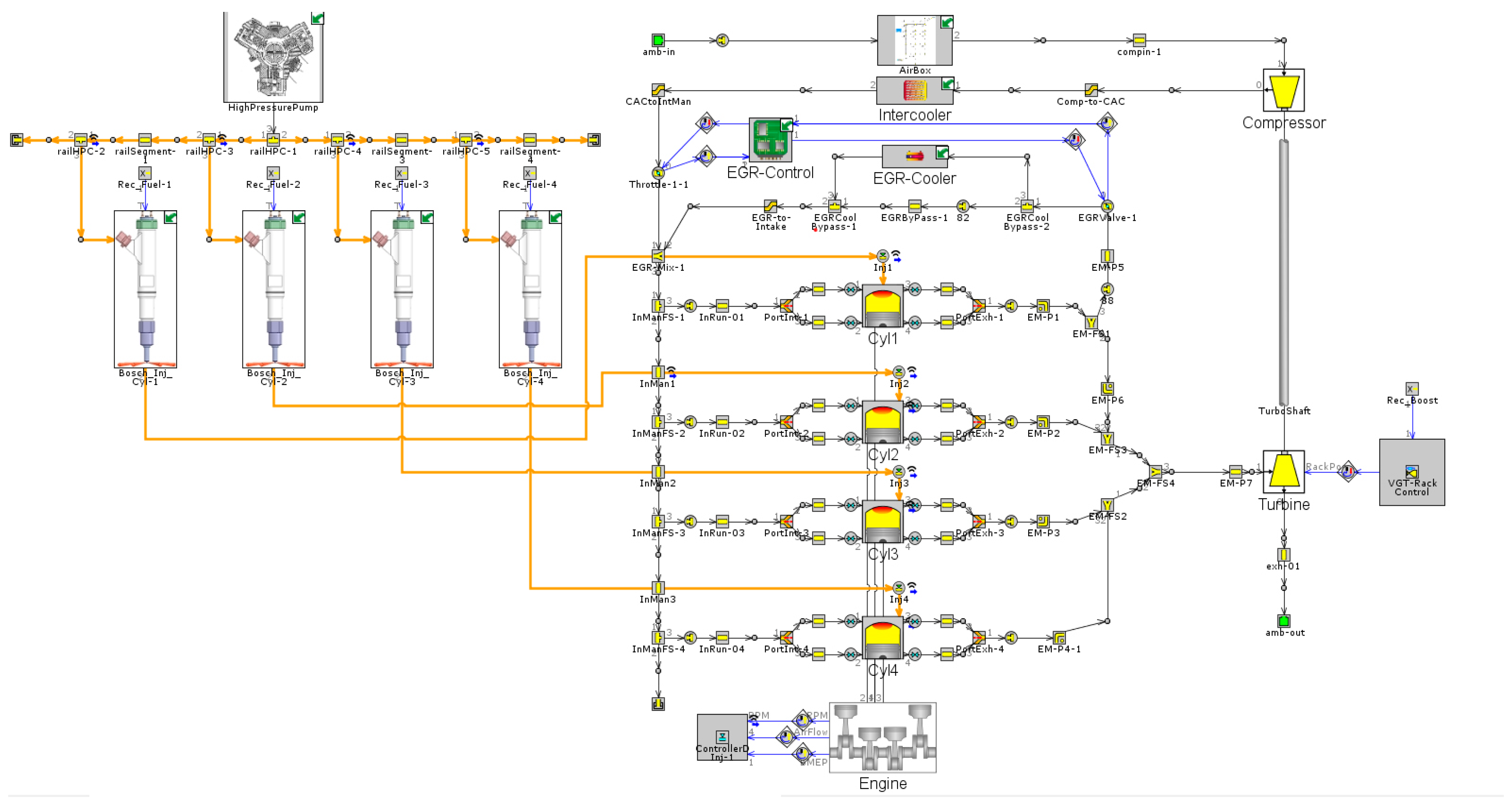
3.4. Establishment of Diesel Engine Simulation Model

The physical model of the engine is primarily divided into three components: the intake system, the cylinder, and the exhaust system. Following the flow sequence of the working medium within the engine, the actual operating process is simplified and standardized into four operational boundary models: the intake system boundary, the cylinder–piston–crankshaft system boundary, the fuel injection system boundary, and the exhaust system boundary, as illustrated in Figure 8.

Figure 9 presents the simulation model of the diesel engine,

Table 1. Key parameters of injector.

Parameter	Specification
Injector Needle Valve Diameter (mm)	10
Injector Nozzle Number × Orifice Diameter (mm)	6 × 0.2
Injector Nozzle Length (mm)	1.5
Injector Injection Pulse Width (ms)	1.8
Injector Pressure Chamber Volume (mm3)	6
Injector Oil Reservoir Volume (mm3)	180
Needle Valve Seat Cone Angle	60°

and

Table 2. Diesel engine-related data.

Name of Engine	Diesel Engine
Fuel	Diesel Fuel
Number of Cylinders	4
Displacement (Volume)	2.149
Max Power	87 kW (Net Power)
Rpm of Max Power	5500
Max Torque	170 Nm (Net Torque)
Rpm of Max Torque	4000 rpm~4400 rpm
Stroke/Diameter	82/91.5
Compression Ratio	18:1
Exhaust Backpressure at Specific Engine RPM (Excluding Converter)	45 kpa@5500

present the key parameters of the injector and the relevant data of the diesel engine.

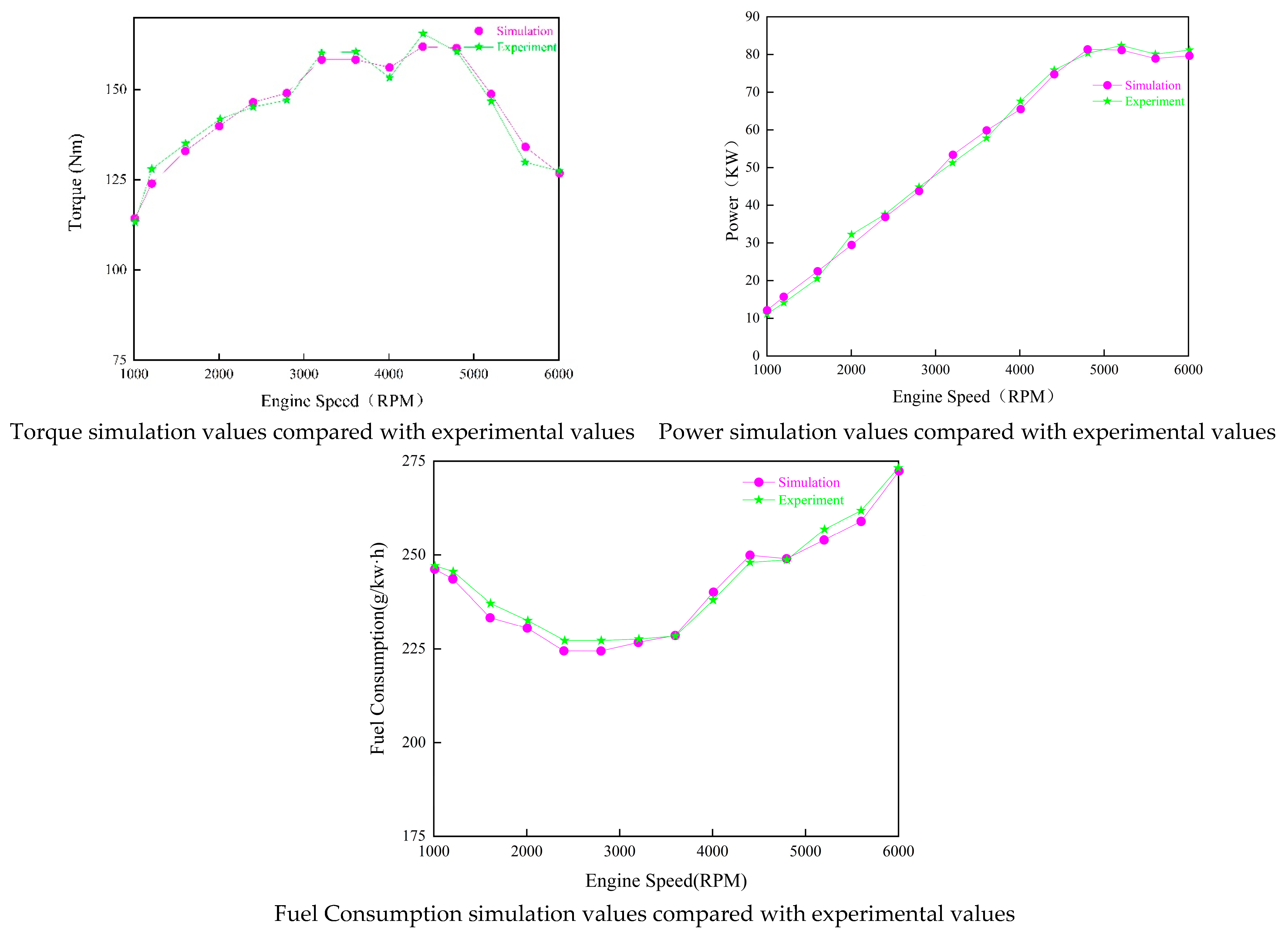
3.5. Coupled Simulation Model and Validation of Electronically Controlled HPCR Fuel Injection System and Diesel Engine System

Using the GT-FLOW module, the diesel engine model developed in GT-POWER is coupled with the HPCR injection system model constructed in GT-FUEL. The coupled model is employed to simulate the effects of key injector structural parameters on pressure fluctuations within the common rail. Compared to simulating the common rail injection system independently, the coupled simulation model based on the actual engine operation process provides a more realistic analysis of pressure fluctuations in the common rail system, as shown in Figure 10.

The accuracy of the model is validated by comparing the simulated external characteristic parameters, such as torque, power, and fuel consumption, with experimental results from the same diesel engine. If significant deviations are observed, the coupled simulation model parameters are adjusted and the simulation is rerun until the discrepancies fall within acceptable limits. The comparative results are depicted in Figure 11.

The results from the above figures indicate that the trends of the simulated torque, power, and fuel consumption curves are generally consistent with the experimental curves. The maximum deviation between the three simulated parameter values and their corresponding experimental values is within 5%. This demonstrates that the simulation model is relatively accurate and confirms that the developed coupled simulation model can be effectively used for simulation studies.

4. The Impact of Fuel Supply Parameters in Electronically Controlled HPCR Injection Systems on Rail Pressure Fluctuations

4.1. Pressure Fluctuations Within the Common Rail During Variations in Fuel Supply Pressure

In the integrated simulation model combining the electronically controlled HPCR injection system with the diesel engine, variations in the supply pressure of the high-pressure fuel pump were analyzed to determine how different inlet pressures affect fluctuations in common rail pressure. The boundary conditions specified numerical pressure values for the high-pressure fuel pump, disregarding the impact of the low-pressure fuel pump on pressure wave propagation. Five distinct low-pressure supply conditions—1 MPa, 2 MPa, 3 MPa, 5 MPa, and 8 MPa—were chosen for detailed simulation and evaluation.

As depicted in Figure 12, the pressure fluctuations in the common rail maintain a consistent pattern throughout a single fuel-supply cycle, irrespective of variations in supply pressure. During the fuel delivery phase, the frequency of pressure oscillations is markedly higher than that observed during the injection phase. This discrepancy arises primarily from the differing time spans of the fuel delivery and injection processes. With an increase in the crankshaft angle, localized pressure variations in the common rail display the following trends: from 0° to 340°, the curve for a supply pressure of 1 MPa reaches its peak, while the 2 MPa curve shows the lowest values; between 340° and 530°, the 8 MPa pressure curve becomes dominant, with the 5 MPa curve at its minimum; and between 530° and 720°, the pressure fluctuation pattern aligns closely with that observed between 0° and 340°. Thus, the common rail pressure does not follow a straightforward, unidirectional pattern with changing supply pressures over a single cycle. Instead, distinct variation trends emerge across different crankshaft angle ranges.

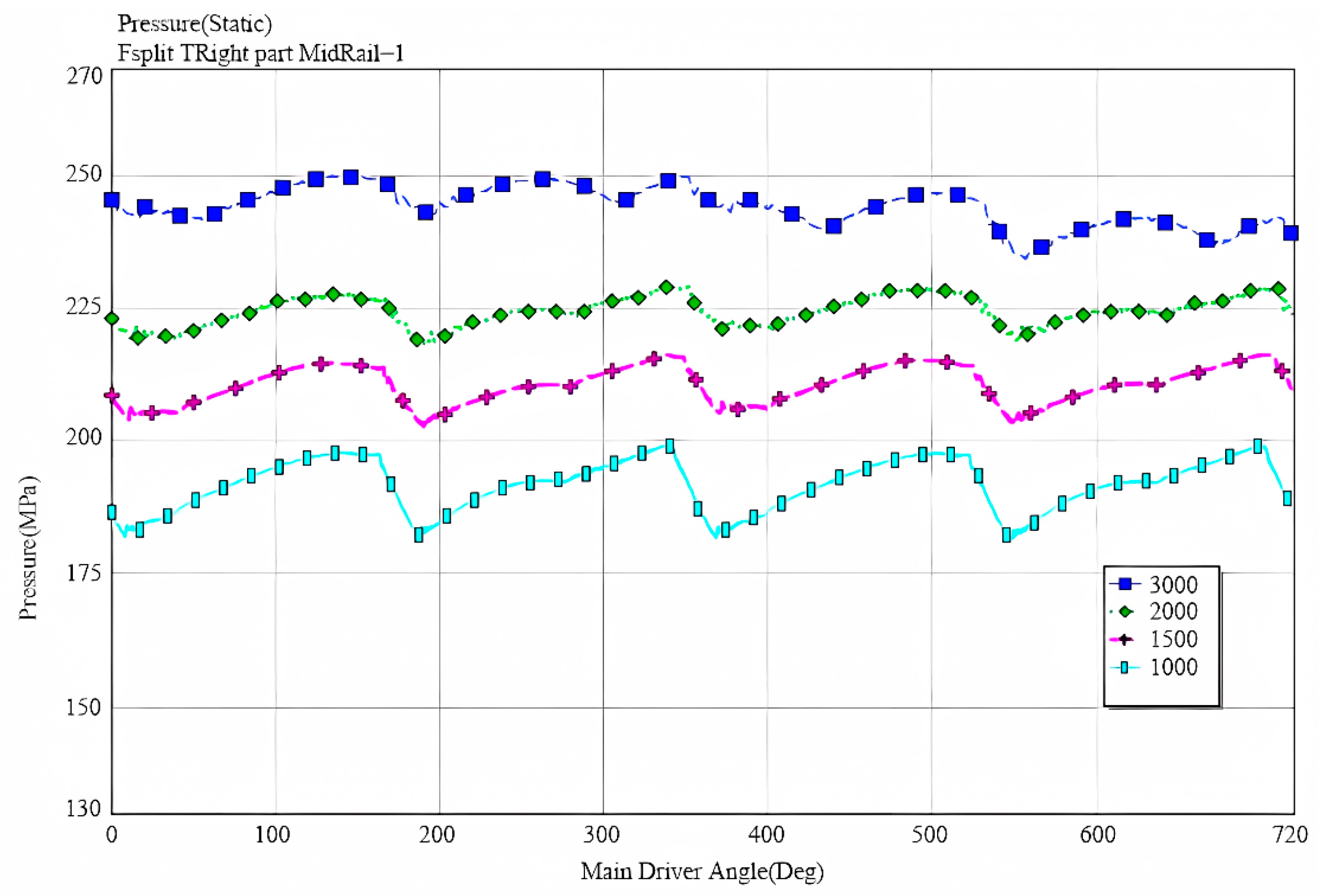
4.2. The Influence of Camshaft Speed on Common Rail Pressure

In the integrated simulation model combining the electronically controlled HPCR injection system with the diesel engine, the rotational speed of the high-pressure fuel pump cam was adjusted to analyze its impact on pressure fluctuations within the common rail. The evaluated cam speeds included 1000 rpm, 1500 rpm, 2000 rpm, and 3000 rpm. Variations in the cam’s rotational velocity inherently modify the plunger’s acceleration profile, thereby affecting the rate of fuel delivery over time and influencing the pressure oscillations within the common rail system.

As illustrated in Figure 13, the pressure behavior within the common rail varies across different rotational speeds. An almost proportional increase in common rail pressure is observed as the speed ratio rises. Furthermore, higher common rail pressures are associated with increased fluctuation frequencies, although the amplitude of these fluctuations generally diminishes. At a constant rotational speed, the pressure curves for odd-numbered and even-numbered fuel supply stages (e.g., 1st and 3rd for odd stages, 2nd and 4th for even stages) exhibit similar patterns within each respective group but differ significantly between the two groups. This discrepancy likely arises from uneven fuel delivery and injection processes. However, at a rotational speed of 3000 rpm, as the crankshaft angle advances, the pressure begins to decline. This drop occurs because the pressure surpasses the threshold defined by the inlet and outlet valve spring parameters under these conditions.

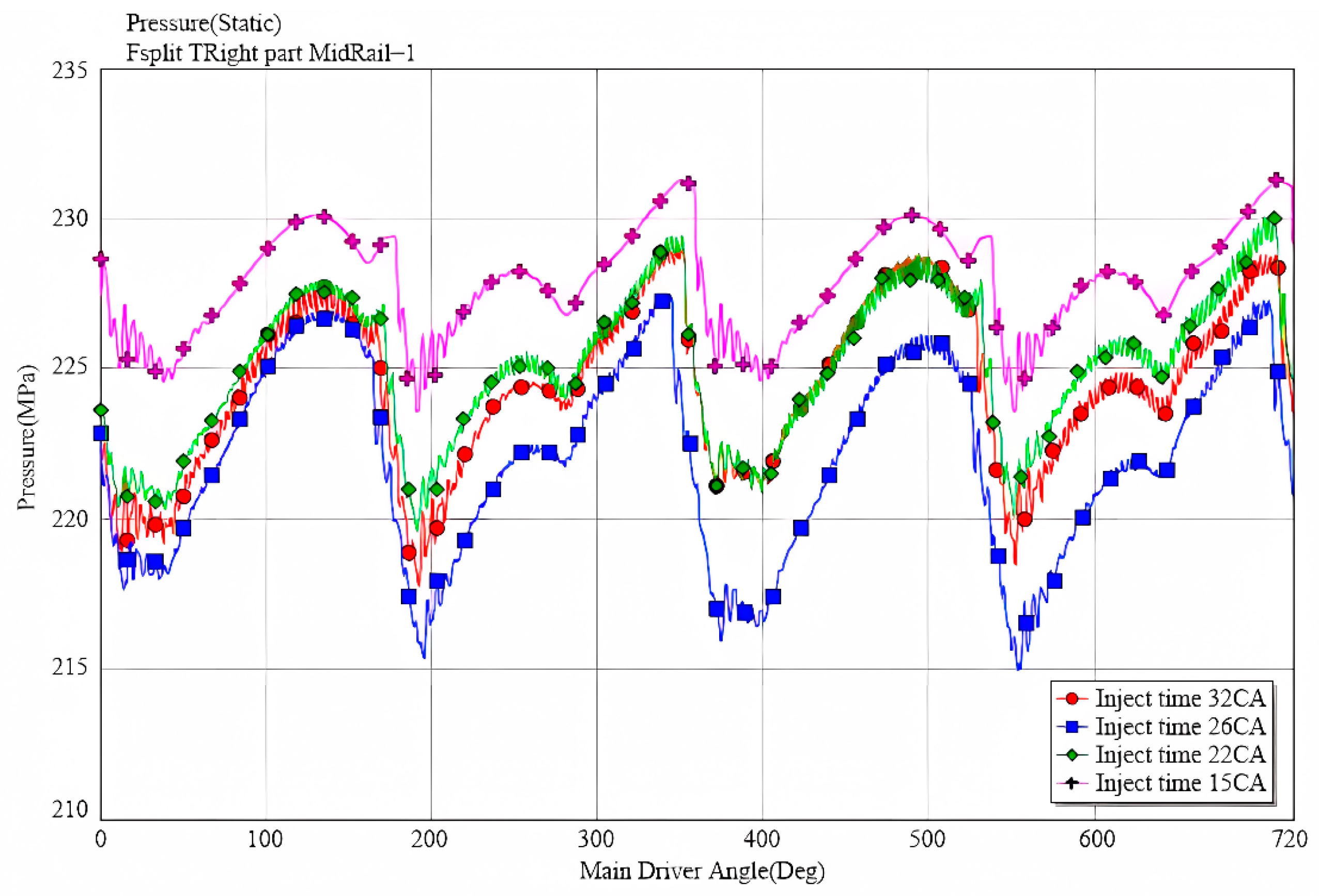
4.3. The Influence of Fuel Injection Pulse Width on Common Rail Pressure

In the established electronically controlled HPCR injection system model, the injector pulse width was varied to investigate its effects on pressure fluctuations within the common rail. The proposed pulse widths were 15 °CA, 22 °CA, 26 °CA, and 32 °CA.

The primary source of pressure fluctuations in a common rail injection system arises from the irregular and variable fuel inflow and outflow within the system. The injector pulse width plays a crucial role in determining both the fuel quantity injected and the injection pattern. As illustrated in Figure 14, increasing the injector pulse width leads to reduced pressure fluctuations in the common rail. This is because a longer pulse width allows more fuel to be injected, which in turn lowers the pressure within the common rail. Furthermore, with extended pulse widths, the injector’s needle valve remains open for a longer period, increasing the time it takes to reach its maximum lift, thereby affecting the pressure fluctuations in the rail. When the pulse width is prolonged, the needle valve gradually achieves its maximum lift. At this point, any further increase in pulse width no longer influences the valve’s opening process but only affects the duration required for it to close [29].

5. The Impact of High-Pressure Oil Pump Plunger Parameter Variations on Rail Pressure Fluctuations

5.1. The Impact of High-Pressure Oil Pump Plunger Mass Variations on Rail Pressure Fluctuations

The mass of the plunger significantly impacts the time required to establish pressure within the plunger chamber, thereby affecting pressure fluctuations in the system. In the developed model, five scenarios with varying plunger masses—85 g, 95 g, 105 g, 115 g, and 125 g—were considered to analyze how changes in plunger mass influence pressure variations in the common rail.

As depicted in Figure 15, an increase in plunger mass results in a slight decrease in common rail pressure. Furthermore, pressure fluctuations within the rail are reduced as the plunger mass grows. This behavior is mainly attributed to the plunger’s higher inertia, which limits the system’s responsiveness to rapid pressure changes. In a high-pressure common rail (HPCR) system, the plunger’s dynamic response plays a crucial role in regulating fuel delivery and injection, ultimately influencing pressure variations within the rail. A heavier plunger requires greater force to accelerate and decelerate, potentially prolonging the time needed for the fuel pump to establish and maintain rail pressure. This extended response time allows the system to stabilize more effectively, thereby reducing the amplitude of pressure fluctuations.

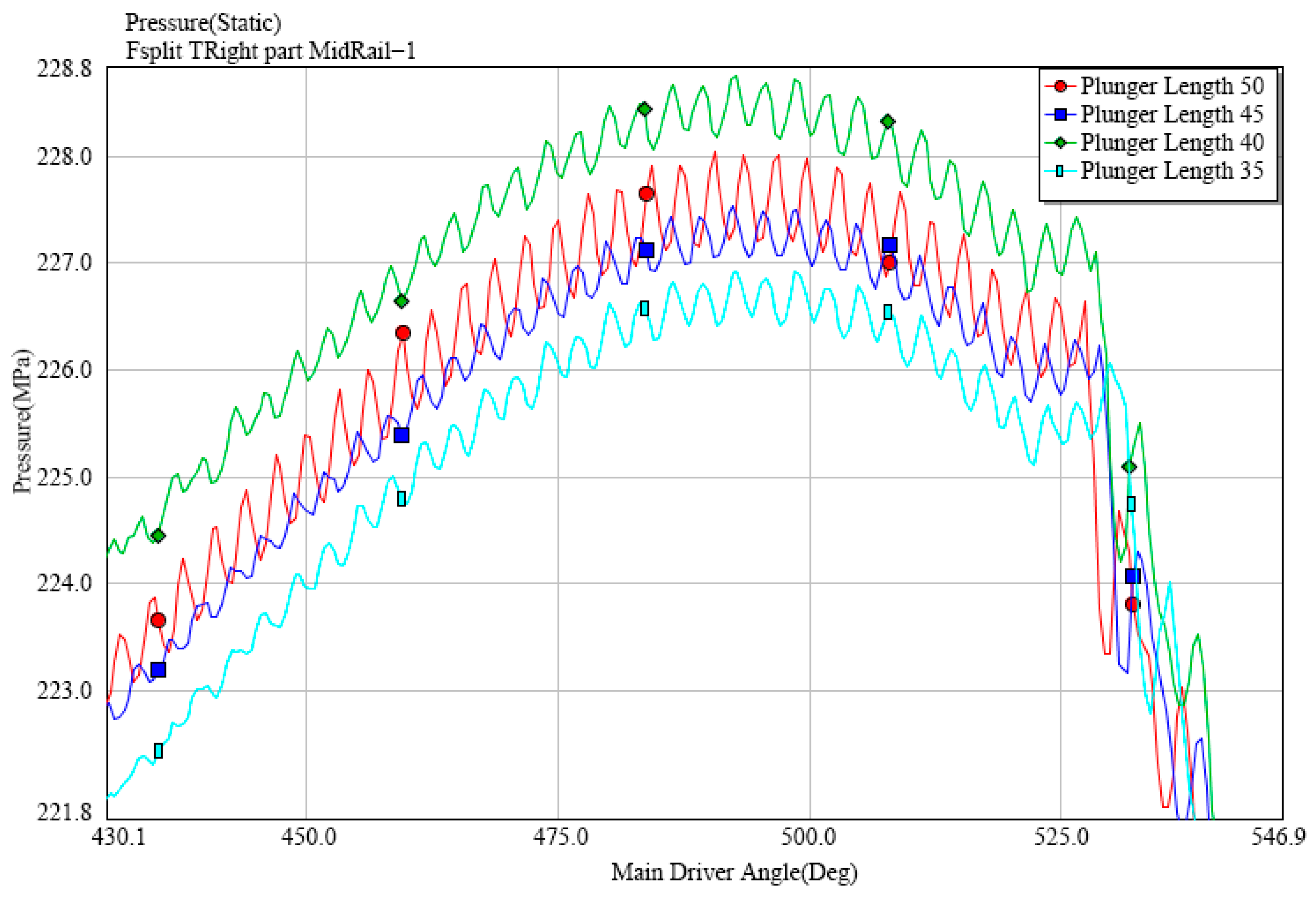
5.2. The Influence of Plunger Length Variations on Rail Pressure Fluctuations

The length of the plunger significantly influences oil pressure variations within the plunger chamber by affecting the sealing performance of the plunger-coupling assembly. This, in turn, determines the extent of oil pressure leakage in the chamber. To examine how changes in plunger length impact pressure fluctuations in the common rail, the model considered four scenarios with plunger lengths of 35 mm, 40 mm, 45 mm, and 50 mm.

As illustrated in Figure 16, extending the plunger length generally results in a slight increase in common rail pressure, with a maximum rise of around 1 MPa. Furthermore, longer plungers lead to higher frequency and amplitude of pressure fluctuations, with the fluctuation amplitude increasing by approximately 0.1 MPa. This behavior is primarily linked to the influence of plunger length on the fuel pump’s displacement capacity; a longer plunger can deliver a greater volume of fuel during each stroke, which may elevate rail pressure and amplify pressure variations. Additionally, variations in plunger length alter its dynamic properties, such as velocity and acceleration, potentially affecting the pump’s operational efficiency and the resulting pressure fluctuations in the rail.

5.3. The Influence of Plunger Spring Preload on Rail Pressure Fluctuations

The preload applied to the plunger spring has a substantial impact on the total force generated by the spring. This force directly acts on the cam, affecting pressure fluctuations in the plunger chamber and ultimately altering the pressure distribution within the common rail. To examine the influence of varying plunger spring preload on these pressure fluctuations, a software model was developed to simulate five scenarios with spring forces set at 1800 N, 1900 N, 2000 N, 2100 N, and 2200 N.

As depicted in Figure 17, increasing the preload of the plunger spring results in a reduction in common rail pressure, with the decrease ranging from 0.5 MPa to 2 MPa. This indicates that the impact on the overall pressure level is relatively minor. Concurrently, the frequency of pressure oscillations in the common rail diminishes as the spring preload rises, leading to a noticeable attenuation of pressure fluctuations. This behavior can be attributed to the enhanced spring force associated with a higher preload, which suppresses pressure variations in the plunger chamber. Consequently, changes in chamber pressure have a reduced ability to influence the plunger’s motion, effectively dampening the pressure oscillations. Moreover, the preload and stiffness of the plunger spring significantly influence the plunger’s dynamic response. A higher preload corresponds to greater spring rigidity, which not only decreases plunger vibrations but also further mitigates fluctuations in rail pressure [30].

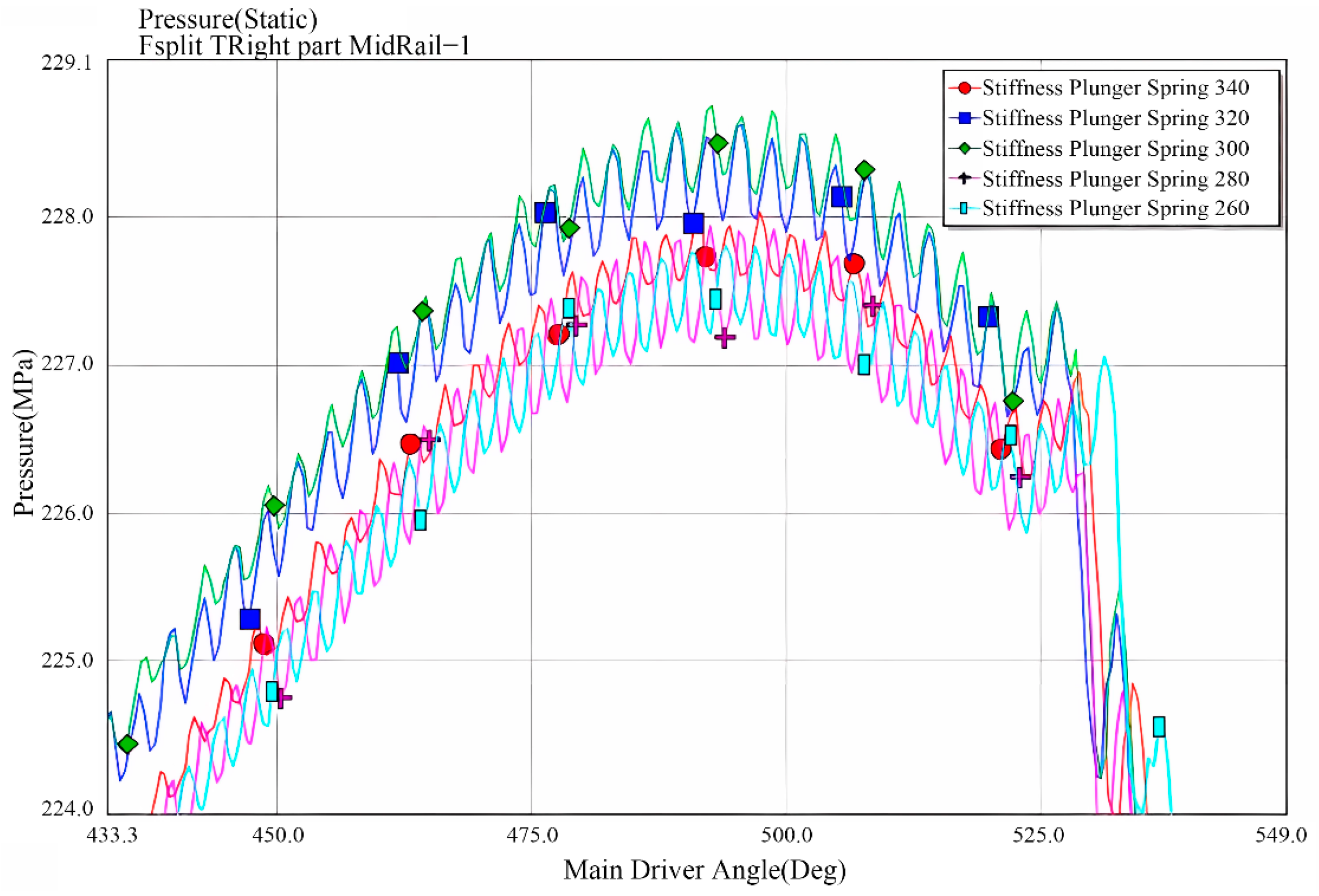
5.4. The Impact of Plunger Spring Stiffness Variation on Rail Pressure Fluctuations

The stiffness of the plunger spring, similar to its preload, exerts a direct influence on the spring force, with variations in stiffness leading to a proportional linear increase in this force. This relationship subsequently impacts the pressure distribution and oscillations within the plunger chamber. To analyze the effect of stiffness changes on pressure fluctuations in the common rail, a software model was designed to simulate five scenarios, using spring stiffness values of 260 N/mm, 280 N/mm, 300 N/mm, 320 N/mm, and 340 N/mm.

As illustrated in Figure 18, increasing the stiffness of the plunger spring leads to a higher frequency of pressure fluctuations in the common rail, accompanied by a slight rise in amplitude. However, this marginal increase has a negligible effect on the overall pressure. Additionally, the pressure curves corresponding to the five selected stiffness values demonstrate similar patterns, suggesting that variations in spring stiffness exert minimal influence on pressure fluctuations. The observed fluctuations arise because spring stiffness governs the plunger’s motion control. Greater stiffness enables a quicker response to plunger movement, thereby reducing pressure variations caused by such a motion. Furthermore, increased stiffness enhances the spring’s capacity to efficiently absorb and release energy, dampening fluctuations driven by plunger activity. In high-pressure common rail (HPCR) systems, tuning spring stiffness plays a pivotal role in optimizing overall system performance.

6. The Impact of Inlet and Outlet Valve Parameters on Pressure Fluctuations Within the HPCR System

6.1. Influence of Mass Variation of the Inlet Valve of High-Pressure Fuel Pump on Common Rail Pressure Fluctuation

The mass of the inlet valve body influences pressure fluctuations in the common rail by affecting its dynamic behavior, energy dissipation, response time, fuel delivery efficiency, and interaction with the valve seat. These factors collectively shape the stability and performance of the high-pressure common rail (HPCR) system [31]. To evaluate the impact of valve body mass on pressure fluctuations, the model examines three scenarios with masses of 0.4 g, 0.6 g, and 0.8 g for the inlet valve body.

As illustrated in Figure 19, the pressure curves within the common rail exhibit consistent overall trends across the three scenarios involving different inlet valve body masses. However, increased pressure fluctuations are observed for valve body masses of 0.4 g and 0.8 g, while the fluctuations are less pronounced for a mass of 0.6 g. This indicates that the pressure response within the common rail does not vary uniformly with changes in valve body mass but instead demonstrates an optimal value. These pressure variations can be attributed to the increased inertia associated with a heavier valve body, which may help stabilize valve motion and subsequently reduce pressure oscillations.

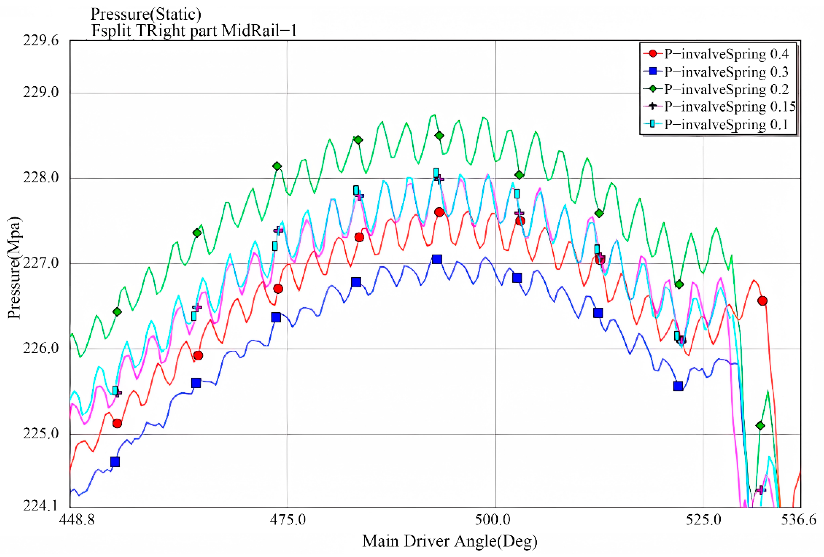
6.2. The Impact of Inlet Valve Spring Preload Variations on Rail Pressure Fluctuations

Variations in the parameters of the inlet valve spring influence the frequency and amplitude of pressure fluctuations in the common rail. Specifically, an increase in the spring’s pre-load force results in reduced frequency and amplitude of these fluctuations. The parameters under consideration include the spring’s pre-load force and stiffness. To examine the effect of pre-load force on pressure waves within the common rail, the model evaluates five scenarios with pre-load forces of 0.1 N, 0.15 N, 0.2 N, 0.3 N, and 0.4 N.

As depicted in Figure 20, increasing the pre-load force of the inlet valve spring results in generally consistent pressure curve trends across the five scenarios. With higher spring pre-load forces, both the frequency and amplitude of pressure fluctuations within the common rail decrease. Notably, between crankshaft angles of 440° and 550°, the pressure reaches its peak at a pre-load force of 0.2 N. This behavior is likely due to the extended opening duration caused by the increased spring force, which helps dampen the pressure variations in the plunger chamber associated with fuel intake.

6.3. The Influence of Inlet Valve Spring Stiffness Variations on Rail Pressure Fluctuations

The stiffness of the inlet valve spring, like its pre-load force, plays a critical role in the valve’s performance. Excessively high stiffness increases the valve’s opening duration, while overly low stiffness delays its seating, potentially leading to an excessive amount of fuel in the plunger chamber. To evaluate how changes in spring stiffness influence pressure waves within the common rail, the model considers five scenarios with stiffness values of 2 N/mm, 2.5 N/mm, 3 N/mm, 4 N/mm, and 5 N/mm.

As illustrated in Figure 21, the pressure within the common rail reaches its lowest point at a spring stiffness of 4 N/mm when the crankshaft angle falls between 450° and 530°, while the highest pressure occurs at a stiffness of 5 N/mm. This suggests that neither excessively low nor excessively high spring stiffness yields optimal performance, indicating the existence of an ideal stiffness value. This behavior can be attributed to the influence of spring stiffness on the system’s dynamic response, as discussed in reference [32].

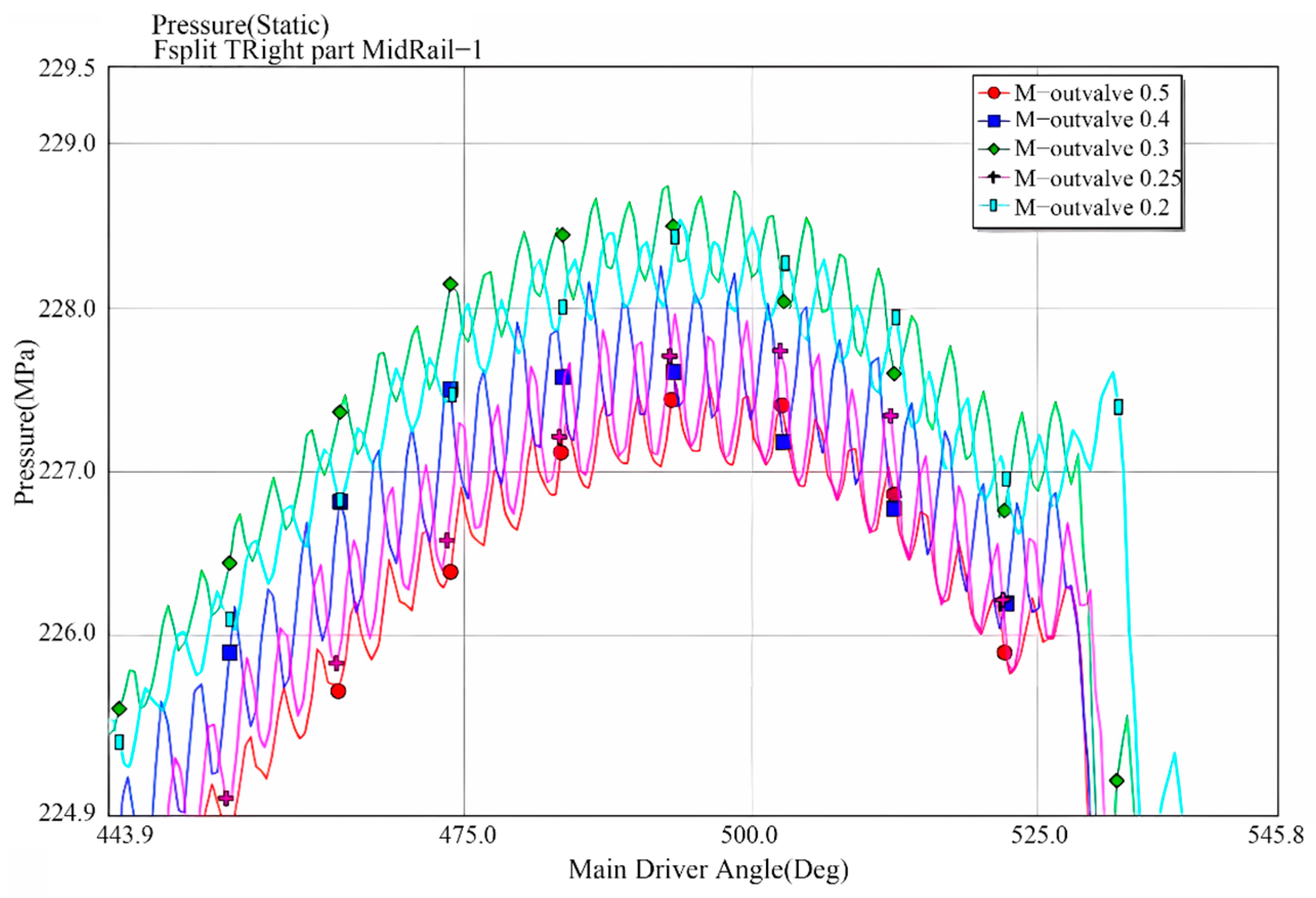
6.4. The Impact of Outlet Valve Body Mass Variations on Rail Pressure Fluctuations in High-Pressure Oil Pumps

The outlet valve serves as the final component responsible for transferring high-pressure fuel from the plunger chamber to the common rail via the high-pressure fuel pipe. By leveraging throttling effects, it moderates pressure fluctuations between the plunger chamber and the common rail, making the pressure waves in the common rail highly sensitive to alterations in the outlet valve’s structural design. Key parameters include the structural attributes of the valve body and the properties of the spring. Changes in the mass of the outlet valve body significantly affect the response times for opening and closing, influencing pressure variations in both the plunger chamber and the common rail. To examine the impact of valve body mass on pressure fluctuations, the model analyzes five scenarios with outlet valve body masses of 0.2 g, 0.25 g, 0.3 g, 0.4 g, and 0.5 g.

As illustrated in Figure 22, the pressure curves within the common rail follow a similar trend across all five scenarios as the crankshaft angle increases, with fluctuations ranging between 0.5 and 3 MPa. Notably, when the outlet valve body mass is 0.5 g, the rail pressure is generally lower compared to other cases. This reduction is likely due to the enhanced damping effect of the heavier valve body, which diminishes fluctuations but may also slow the valve’s response. During the later stages of fuel delivery, more pronounced pressure fluctuations are observed within the common rail when the valve body mass is 0.2 g. This behavior can be attributed to the cumulative pressure effect in the rail, where lighter valve bodies are less effective at mitigating pressure surges.

6.5. The Impact of Outlet Valve Spring Pre-Tightening Force Variations on Rail Pressure Fluctuations in High-Pressure Oil Pumps

Similarly to the inlet valve, the preload of the outlet valve spring must be carefully optimized. Excessive preload delays the valve’s opening, whereas insufficient preload leads to unstable valve seating, both of which negatively impact the fuel supply efficiency of the high-pressure pump. To examine how variations in spring preload influence pressure fluctuations within the common rail, the model considers five scenarios with preload values of 0.05 N, 0.08 N, 0.1 N, 0.2 N, and 0.3 N.

As depicted in Figure 23, the pressure curves within the common rail exhibit a generally consistent trend across the five scenarios as the crankshaft angle increases, with only minor pressure variations. However, in the final phase, the pressures are highest when the outlet valve spring preload is set to 0.05 N and 0.3 N, with the pressure curves for these cases nearly overlapping. This suggests that the influence of spring preload on rail pressure is not linear. A detailed analysis reveals that both excessively high and low preload values adversely affect pressure stability, emphasizing the importance of achieving an optimal balance.

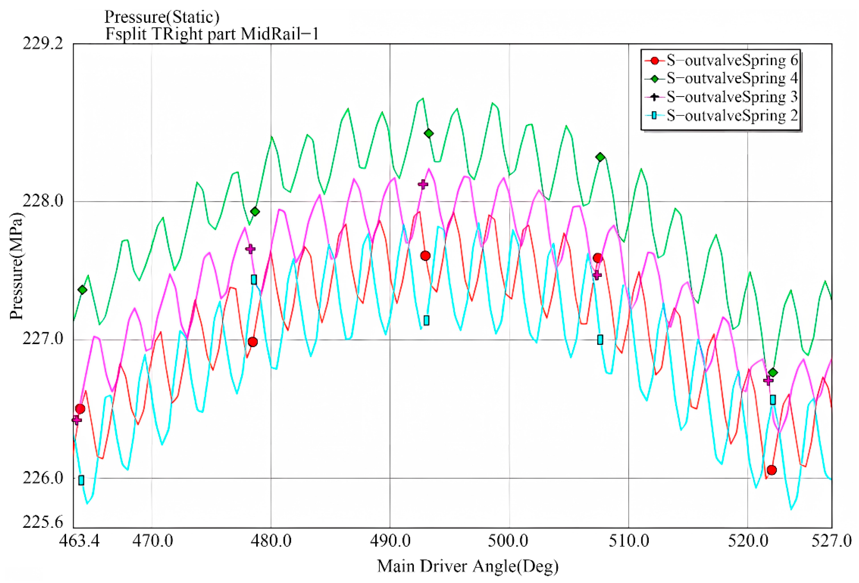
6.6. The Impact of Outlet Valve Spring Stiffness Variations on Rail Pressure Fluctuations

Similarly to the preload, the stiffness of the outlet valve spring also affects pressure fluctuations in both the plunger chamber and the common rail. In the established model, four scenarios were designed with outlet valve spring stiffness values of 2 N/mm, 3 N/mm, 4 N/mm, and 6 N/mm to investigate the impact of spring stiffness variations on pressure fluctuations within the common rail.

As illustrated in Figure 24, the pressure curves within the common rail demonstrate similar patterns across the four scenarios as the crankshaft angle increases, showing minimal variation and a reduction in fluctuation frequency. Notably, the smallest fluctuation amplitude occurs when the outlet valve spring stiffness is 4 N/mm, whereas larger amplitudes are observed in other cases. This behavior is linked to the increased responsiveness of the outlet valve with greater spring stiffness, which enhances fuel quantity regulation, minimizes fluctuations, and contributes to maintaining or boosting rail pressure [33].

7. Gray Relation Analysis (GRA)

Gray relational analysis is a mathematical method used to evaluate the relationships between various factors in a system, particularly suitable for situations where data are incomplete, uncertain, or insufficiently available [34]. This method determines the degree of association between system factors based on the geometric similarity of patterns. By comparing the differences between the reference sequence (parent sequence) and the comparison sequence (subsequence), the relational degree is calculated, which in turn assesses their similarity or correlation [35]. In this study, gray relational analysis is applied to investigate the correlation between outlet valve spring stiffness and inlet valve spring stiffness, as well as between outlet valve spring preload and inlet valve spring preload, in relation to the pressure within the rail. The main calculation steps are as follows:

(1)

Determine the Analysis Sequence

Select one or more reference sequences (parent sequences) and several comparison data sequences (subsequences). The parent sequence represents the data sequence reflecting the behavioral characteristics of the system, while the subsequences consist of data sequences representing factors influencing the system’s behavior. The reference sequence for the gray relational analysis is as follows:

($\mathrm{Y}$) represents the reference sequence.

$$\mathrm{Y}=\left\{\mathrm{Y}(\mathrm{i},\mathrm{j})|\mathrm{i} ,\mathrm{j}=1, 2, 3, \cdots ,\mathrm{n}\right\}$$

(25)

The comparative sequences for the gray relational problem are as follows:

$$\mathrm{X}=\left\{\mathrm{X}(\mathrm{i},\mathrm{j})|\mathrm{i} ,\mathrm{j}=1, 2, 3, \cdots ,\mathrm{n}\right\}$$

(26)

where ($\mathrm{X}$) represents the comparison sequences, which in this study include the outlet valve spring stiffness and inlet valve spring stiffness, as well as the outlet valve spring preload and inlet valve spring preload.

(2)

Data Preprocessing of Variables

In practical problems, data may exhibit varying attributes and dimensions. To ensure that the original data meets the requirements of fuzzy clustering, normalization of the original data matrix is necessary [16]. The mean value of each indicator is first calculated, and each element within the indicator is then divided by its respective mean. The resulting standardized matrix is denoted as ($\mathrm{Z}$), with its elements represented as (${\mathrm{Z}}_{\mathrm{i}\mathrm{j}}$).

$${\mathrm{Z}}_{\mathrm{i}\mathrm{j}}={\displaystyle \frac{{\mathrm{X}}_{\mathrm{i}\mathrm{j}}}{\overline{{\mathrm{X}}_{\mathrm{i}\mathrm{j}}}}}$$

(27)

(3)

Calculating the Correlation Coefficients between Subsequence Indicators and the Reference Sequence

The gray correlation coefficient between the reference series and each comparison series is calculated using the following formula, which yields a parametric measurement of the correlation between the comparison series and the reference series. By comparing the values, the correlation ranking of each parameter in the system can be determined [16].

$$\mathrm{Y}({\mathrm{X}}_0(\mathrm{k}),{\mathrm{X}}_{\mathrm{i}}(\mathrm{k}))={\displaystyle \frac{\mathrm{a}+\rho \mathrm{b}}{\left|{\mathrm{X}}_0(\mathrm{K})\right|–\left|{\mathrm{X}}_{\mathrm{i}}(\mathrm{K})\right|+\rho \mathrm{b}}}(\mathrm{i}=1,2,\cdots ,\mathrm{m},\mathrm{k}=1,2,\cdots ,\mathrm{n})$$

(28)

$$\begin{array}{l}\mathrm{a}={\min }_{\mathrm{i}}{\min }_{\mathrm{k}}\left|{\mathrm{X}}_0(\mathrm{k})–{\mathrm{X}}_{\mathrm{i}}(\mathrm{k})\right|\\ \mathrm{b}={\max }_{\mathrm{i}}{\max }_{\mathrm{k}}\left|{\mathrm{X}}_0(\mathrm{k})–{\mathrm{X}}_{\mathrm{i}}(\mathrm{k})\right|\end{array}$$

(29)

In this context, ($\mathrm{a}$) represents the minimum values between two levels, ($\mathrm{b}$) represents the maximum values between two levels, and ($\rho$) is the discrimination coefficient (commonly taken as 0.5); in this paper, it is taken as 0.5.

(4)

Calculation of Gray Relational Degree

In this paper, ($\mathrm{Y}({\mathrm{X}}_0,{\mathrm{X}}_{\mathrm{i}})$) is defined as the gray relational degree, which is obtained by averaging the correlation coefficients matrix column by column.

$$\mathrm{Y}({\mathrm{X}}_0,{\mathrm{X}}_{\mathrm{i}})={\displaystyle \frac{1}{\mathrm{n}}}{\displaystyle \sum _{\mathrm{k}=1}^{\mathrm{n}}\mathrm{Y}({\mathrm{X}}_0(\mathrm{k}),{\mathrm{X}}_{\mathrm{i}}(\mathrm{k}))}$$

(30)

This study employed MATLAB 2018a for computational analysis, aiming to streamline the calculation process and enhance accuracy. The results indicate the influence of the inlet valve spring preload, outlet valve spring preload, inlet valve spring stiffness, and outlet valve spring stiffness on rail pressure fluctuations, with gray correlation degrees of 0.815, 0.551, 0.625, and 0.527, respectively. These data reveal that the inlet valve spring preload has the strongest correlation with rail pressure fluctuations, followed by the inlet valve spring stiffness. In contrast, the outlet valve spring preload and stiffness have relatively lower impacts. This finding suggests that among these four factors, adjusting the inlet valve spring preload yields the most significant effect.

8. Conclusions

This paper first establishes a fluid control model for the HPCR system, as well as mathematical models for the high-pressure fuel pump, common rail pipe, and injector, laying the theoretical foundation for subsequent simulation analysis. Then, based on the GT-Fuel submodule of GT-Suite software, simulation models for the high-pressure fuel pump, common rail pipe, and solenoid valve injector are created. The software’s Assembly function is used to combine these three components into a complete HPCR system. To improve the authenticity and effectiveness of the simulation model, a diesel engine simulation model is developed using the GT-Power submodule of GT-Suite. Finally, the HPCR system model is coupled with the diesel engine model using the software, forming a comprehensive simulation model. To validate the accuracy of the simulation model, the data obtained from the simulation is compared with experimental data, confirming the model’s accuracy. The paper further investigates the impact of three main factors—fuel supply parameters of the HPCR injection system, plunger parameters of the high-pressure fuel pump, and the parameters of the inlet and outlet valves of the high-pressure fuel pump—on rail pressure fluctuations. Additionally, using the gray correlation analysis method, the correlation between each parameter and rail pressure fluctuation is quantified. The specific research findings are as follows:

(1)

Through the analysis of the impact of fuel supply parameters in the high-pressure common rail fuel injection system on the rail pressure fluctuation, it was found that the fuel supply pressure, camshaft speed, and injection pulse width all have significant effects on rail pressure fluctuations. At different fuel supply pressures, the pressure fluctuation frequency during the fuel supply phase is higher than that during the injection phase. As the camshaft speed increases, the common rail pressure increases proportionally, with the fluctuation frequency rising and the amplitude decreasing. Specifically, the ratio of the common rail pressure at a camshaft speed of 3000 rpm to that at 2000 rpm is approximately 1.11. Increasing the injection pulse width results in a reduction in the pressure fluctuation amplitude within the common rail. When the injection pulse width is 32 CA, the amplitude of pressure fluctuation decreases by approximately 3 MPa compared to when the pulse width is 26 CA.

(2)

By analyzing the influence of plunger parameter variations in a high-pressure fuel pump on rail pressure fluctuations, it was found that changes in the plunger’s mass and length affect rail pressure oscillations. An increase in plunger mass results in a reduction in the rail pressure. When the plunger length increases, both the frequency and amplitude of rail pressure fluctuations rise slightly, with a maximum amplitude increase of approximately 1 MPa. Simultaneously, the increased plunger length elevates the fluctuation frequency and amplitude of rail pressure, though the amplitude increase is limited to around 0.1 MPa. Additionally, an increase in the preload of the plunger spring leads to a decreasing trend in rail pressure, with the reduction varying between 0.5 MPa and 2 MPa, while the amplitude of pressure fluctuations also decreases. Conversely, variations in the plunger spring stiffness exhibit a relatively minor effect on rail pressure fluctuations.

(3)

Examination of the effects of inlet and outlet valve parameter variations in the high-pressure fuel pump on rail pressure fluctuations demonstrated that the valve body mass, spring preload, and spring stiffness of the valves all influence rail pressure fluctuations. Gray correlation analysis indicated that the spring preload of the inlet valve has the highest correlation with rail pressure fluctuations (0.815), followed by the spring stiffness of the inlet valve (0.625), while the spring preload (0.551) and spring stiffness (0.527) of the outlet valve have relatively lower correlations. This suggests that optimizing the inlet valve spring preload is the most critical factor for reducing rail pressure fluctuations.

References

1. Ahire, V.; Shewale, M.; Razban, A. A review of the state-of-the-art emission control strategies in modern diesel engines. Arch. Comput. Methods Eng. 2021, 28, 4897–4915. [Google Scholar] [CrossRef]
2. Hoang, A.T. Applicability of fuel injection techniques for modern diesel engines. In Proceedings of the AIP Conference Proceedings; AIP Publishing: Melville, NY, USA, 2020. [Google Scholar]
3. Varshil, P.; Deshmukh, D. A comprehensive review of waste heat recovery from a diesel engine using organic rankine cycle. Energy Rep. 2021, 7, 3951–3970. [Google Scholar]
4. Alwi, E.; Amin, B.; Afnison, W. Electric turbo compounding (ETC) as exhaust energy recovery system on vehicle. GEOMATE J. 2020, 19, 228–234. [Google Scholar]
5. Jiang, F.; Zhou, J.; Hu, J.; Tan, X.; Mo, Q.; Cao, W. Performance Comparison and Optimization of 16V265H Diesel Engine Fueled with Biodiesel Based on Miller Cycle. Processes 2022, 10, 1412. [Google Scholar] [CrossRef]
6. Song, L.; Liu, T.; Fu, W.; Lin, Q. Experimental study on spray characteristics of ethanol-aviation kerosene blended fuel with a high-pressure common rail injection system. J. Energy Inst. 2018, 91, 203–213. [Google Scholar] [CrossRef]
7. Shatrov, M.G.; Dunin, A.U.; Dushkin, P.V.; Yakovenko, A.L.; Golubkov, L.N.; Sinyavski, V.V. Influence of pressure oscillations in common rail injector on fuel injection rate. Facta Univ. Ser. Mech. Eng. 2020, 18, 579–593. [Google Scholar] [CrossRef]
8. Hu, Y.; Yang, J.; Hu, N. Experimental study and optimization in the layouts and the structure of the high-pressure common-rail fuel injection system for a marine diesel engine. Int. J. Engine Res. 2021, 22, 1850–1871. [Google Scholar] [CrossRef]
9. Liu, Y.; Zhang, Y.-T.; Qiu, T.; Ding, X.; Xiong, Q. Optimization research for a high pressure common rail diesel engine based on simulation. Int. J. Automot. Technol. 2010, 11, 625–636. [Google Scholar] [CrossRef]
10. Yang, X.; Dong, Q.; Song, J.; Zhou, T. Investigation of a method for online measurement of injection rate for a high-pressure common rail diesel engine injector under multiple-injection strategies. Meas. Sci. Technol. 2021, 33, 025301. [Google Scholar] [CrossRef]
11. Qi, B.; Zhang, Y.; Guo, D. Study on seal performance of injector nozzle in high-pressure common rail injection system. J. Braz. Soc. Mech. Sci. Eng. 2018, 40, 1–10. [Google Scholar] [CrossRef]
12. Gao, Z.-G.; Li, G.-X.; Xu, C.-l.; Li, H.-M.; Wang, M. Simulation study on pressure fluctuation characteristics of a high-pressure common rail system. Proc. Inst. Mech. Eng. Part D J. Automob. Eng. 2023, 237, 2645–2663. [Google Scholar] [CrossRef]
13. Xu, L.; Bai, X.-S.; Jia, M.; Qian, Y.; Qiao, X.; Lu, X. Experimental and modeling study of liquid fuel injection and combustion in diesel engines with a common rail injection system. Appl. Energy 2018, 230, 287–304. [Google Scholar] [CrossRef]
14. Wei, Y.; Fan, L.; Wu, Y.; Gu, Y.; Xu, J.; Fei, H. Research on transmission and coupling characteristics of multi-frequency pressure fluctuation of high pressure common rail fuel system. Fuel 2022, 312, 122632. [Google Scholar] [CrossRef]
15. Agarwal, A.K.; Singh, A.P.; Maurya, R.K.; Shukla, P.C.; Dhar, A.; Srivastava, D.K. Combustion characteristics of a common rail direct injection engine using different fuel injection strategies. Int. J. Therm. Sci. 2018, 134, 475–484. [Google Scholar] [CrossRef]
16. Jiang, H.; Wang, H.; Jiang, F.; Hu, J.; Hu, L. Research on the Optimization of a Diesel Engine Intercooler Structure Based on Numerical Simulation. Processes 2024, 12, 276. [Google Scholar] [CrossRef]
17. Danilevičius, A.; Karpenko, M.; Křivánek, V. Research on the noise pollution from different vehicle categories in the urban area. Transport 2023, 38, 1–11. [Google Scholar] [CrossRef]
18. Bai, Y.; Lan, Q.; Fan, L.; Ma, X.; Liu, H. Investigation on the fuel injection stability of high pressure common rail system for diesel engines. Int. J. Engine Res. 2021, 22, 616–631. [Google Scholar] [CrossRef]
19. Li, P.; Zhang, Y.; Li, T.; Xie, L. Elimination of fuel pressure fluctuation and multi-injection fuel mass deviation of high pressure common-rail fuel injection system. Chin. J. Mech. Eng. 2015, 28, 294–306. [Google Scholar] [CrossRef]
20. Niklawy, W.; Shahin, M.; Amin, M.; Elmaihy, A. Modelling and experimental investigation of high–pressure common rail diesel injection system. In Proceedings of the IOP Conference Series: Materials Science and Engineering; IOP Publishing: Bristol, UK, 2020; p. 012037. [Google Scholar]
21. Lan, Q.; Bai, Y.; Fan, L.; Gu, Y.; Wen, L.; Yang, L. Investigation on fuel injection quantity of low-speed diesel engine fuel system based on response surface prediction model. Energy 2020, 211, 118946. [Google Scholar] [CrossRef]
22. Wang, D.; Xu, Z.; Su, C.; Hu, J. Pressure Control Strategy and Simulation of High Pressure Common Rail System. J. Phys. Conf. Ser. 2020, 1624, 022061. [Google Scholar]
23. Li, Z.; Wang, Y.; Yin, Z.; Gao, Z.; Wang, Y.; Zhen, X. An exploratory numerical study of a diesel/methanol dual-fuel injector: Effects of nozzle number, nozzle diameter and spray spacial angle on a diesel/methanol dual-fuel direct injection engine. Fuel 2022, 318, 123700. [Google Scholar] [CrossRef]
24. Balz, R.; von Rotz, B.; Sedarsky, D. In-nozzle flow and spray characteristics of large two-stroke marine diesel fuel injectors. Appl. Therm. Eng. 2020, 180, 115809. [Google Scholar] [CrossRef]
25. Gupta, P.; Rajak, U.; Verma, T.N.; Arya, M.; Singh, T.S. Impact of fuel injection pressure on the common rail direct fuel injection engine powered by microalgae, kapok oil, and soybean biodiesel blend. Ind. Crops Prod. 2023, 194, 116332. [Google Scholar] [CrossRef]
26. He, Z.; Zhou, H.; Duan, L.; Xu, M.; Chen, Z.; Cao, T. Effects of nozzle geometries and needle lift on steadier string cavitation and larger spray angle in common rail diesel injector. Int. J. Engine Res. 2021, 22, 2673–2688. [Google Scholar] [CrossRef]
27. Ning, L.; Duan, Q.; Chen, Z.; Kou, H.; Liu, B.; Yang, B.; Zeng, K. A comparative study on the combustion and emissions of a non-road common rail diesel engine fueled with primary alcohol fuels (methanol, ethanol, and n-butanol)/diesel dual fuel. Fuel 2020, 266, 117034. [Google Scholar] [CrossRef]
28. Liu, J.; Liu, Z.; Wang, L.; Wang, P.; Sun, P.; Ma, H.; Wu, P. Effects of PODE/diesel blends on particulate matter emission and particle oxidation characteristics of a common-rail diesel engine. Fuel Process. Technol. 2021, 212, 106634. [Google Scholar] [CrossRef]
29. Bai, Y.; Chen, Z.; Dou, W.; Kong, X.; Yao, J.; Ai, C.; Zhai, F.; Zhang, J.; Yang, L. Pressure Fluctuation Characteristics of High-Pressure Common Rail Fuel Injection System. Diesel Engines Biodiesel Engines Technol. 2022, 2022, 229. [Google Scholar]
30. Li, R.; Yuan, W.; Xu, J.; Wang, L.; Chi, F.; Wang, Y.; Liu, S.; Lin, J.; Zhang, Q.; Chen, L. Study of the Optimization of Rail Pressure Characteristics in the High-Pressure Common Rail Injection System for Diesel Engines Based on the Response Surface Methodology. Processes 2023, 11, 2626. [Google Scholar] [CrossRef]
31. Fayad, M.A.; Al-Salihi, H.A.; Dhahad, H.A.; Mohammed, F.M.; Al-Ogidi, B.R. Effect of post-injection and alternative fuels on combustion, emissions and soot nanoparticles characteristics in a common-rail direct injection diesel engine. Energy Sources Part A Recovery Util. Environ. Eff. 2021, 3, 1–15. [Google Scholar] [CrossRef]
32. Chen, G.; Chen, C.; Yuan, Y.; Zhu, L. Modelling and simulation analysis of high-pressure common rail and electronic controlled injection system for diesel engine. Appl. Math. Nonlinear Sci. 2020, 5, 345–356. [Google Scholar] [CrossRef]
33. Wenbin, C.; Ruilin, M.; Yinshui, L.; Defa, W.; Xiaowen, C. Effects of distribution valve spring stiffness and opening pressure on the volumetric efficiency of micro high-pressure plunger pump. Adv. Mech. Eng. 2024, 16, 16878132241288404. [Google Scholar] [CrossRef]
34. Abifarin, J.; Ofodu, J. Modeling and grey relational multi-response optimization of chemical additives and engine parameters on performance efficiency of diesel engine. Int. J. Grey Syst. 2022, 2, 16–26. [Google Scholar] [CrossRef]
35. Muqeem, M.; Sherwani, A.F.; Ahmad, M.; Khan, Z.A. Taguchi based grey relational analysis for multi response optimisation of diesel engine performance and emission parameters. Int. J. Heavy Veh. Syst. 2020, 27, 441–460. [Google Scholar] [CrossRef]
Figure 1. The structure of this paper.
Energies 18 00550 g001
Figure 2. Schematic diagram of the HPCR fuel injection system configuration.
Energies 18 00550 g002
Figure 3. Physical model of high-pressure oil pump.
Energies 18 00550 g003
Figure 4. High-pressure oil pump simulation model diagram.
Energies 18 00550 g004
Figure 5. Physical model of fuel injector.
Energies 18 00550 g005
Figure 6. Fuel injector simulation model.
Energies 18 00550 g006
Figure 7. Overall simulation model diagram of electronically controlled HPCR fuel injection system.
Energies 18 00550 g007
Figure 8. Engine physical model diagram.
Energies 18 00550 g008
Figure 9. Diesel engine simulation model diagram.
Energies 18 00550 g009
Figure 10. Coupled simulation model.
Energies 18 00550 g010
Figure 11. Simulation-Experimental Validation Comparison.
Energies 18 00550 g011
Figure 12. The impact of fuel supply pressure on common rail pressure.
Energies 18 00550 g012
Figure 13. Pressure variations within the common rail at different camshaft speeds.
Energies 18 00550 g013
Figure 14. The impact of different injection pulse widths on common rail pressure.
Energies 18 00550 g014
Figure 15. The impact of plunger mass variations on common rail pressure.
Energies 18 00550 g015
Figure 16. The impact of different plunger lengths on common rail pressure.
Energies 18 00550 g016
Figure 17. The influence of plunger spring preload on common rail pressure.
Energies 18 00550 g017
Figure 18. The influence of plunger spring stiffness on common rail pressure.
Energies 18 00550 g018
Figure 19. The impact of variations in inlet valve mass on rail pressure.
Energies 18 00550 g019
Figure 20. The influence of different inlet valve spring preload on rail pressure.
Energies 18 00550 g020
Figure 21. The impact of different inlet valve spring stiffness on rail pressure.
Energies 18 00550 g021
Figure 22. The impact of different outlet valve body mass on rail pressure.
Energies 18 00550 g022
Figure 23. The impact of different outlet valve spring preload on rail pressure.
Energies 18 00550 g023
Figure 24. The impact of different outlet valve spring stiffness on rail pressure.
Energies 18 00550 g024