Discussion on AC Resistance and Temperature of ACSR Based on Finite Element Model Assistance

Abstract

In overhead wire transmission systems, the presence of AC resistance results in increased energy dissipation, adversely affecting the lines’ capacity to conduct current. This paper employs a finite element aluminum conductor steel-reinforced (ACSR) model, combined with electrical measurement techniques, to investigate AC resistance. By applying varying levels of AC current, the model is employed to determine the AC resistance which closely aligns with theoretical values estimated using the Morgan algorithm. The trends observed in the parameters are consistent, thereby validating the accuracy of the model. Following simulations and analyses regarding both AC resistance and temperature variations within the conductors—and incorporating empirical measurement results—it is demonstrated that, when environmental factors are not considered, any increase in the conductor temperature can be integrated into a revised model. This updated model is subsequently compared against test results obtained from an experimental platform; the findings confirm that the estimation errors remain within an acceptable range. Overall, this simulation model serves as a valuable reference for assessing AC losses in existing conductors, as well as contributing to reduced experimental costs while mitigating the associated risks and challenges. In summary, this simulation model serves as an essential reference for assessing AC losses in current conductors and aids in reducing experimental costs while addressing the associated risks and challenges.

1. Introduction

By measuring the AC resistivity of an ACSR model, it is possible to evaluate and select wires with a lower resistivity, thereby reducing power loss during transmission. This measurement not only facilitates the selection of wires with an enhanced conductivity, but also improves overall transmission efficiency [1,2]. For instance, high-conductivity steel-core aluminum stranded wire can achieve approximately a 3% reduction in losses compared to conventional wires [3]. Furthermore, assessing AC resistivity enables the optimization of line design and supports the selection of more suitable wire specifications and structures tailored to specific transmission requirements and environmental conditions. For example, utilizing lightweight wires for ultra-high voltage transmission lines can decrease both the weight of the conductors themselves and their outer diameter. This reduction subsequently alleviates wind pressure loads on towers, resulting in lighter tower structures and cost savings [4]. Additionally, measuring AC resistivity provides valuable insights into the energy-saving advantages associated with different materials. The implementation of ACSR wire effectively reduces DC resistance while minimizing hysteresis and eddy current losses within the steel core; this further contributes to a decrease in AC resistance [5]. In summary, measuring the AC resistivity of ACSR wire is essential for enhancing transmission efficiency, minimizing losses, optimizing line design, evaluating energy-saving benefits, and ensuring electromagnetic environment safety.

In both laboratory and industrial settings, the primary methodologies for assessing the AC resistance of conductors are generally categorized into the following two distinct groups: those based on thermal principles and those that employ electrical principles [6,7]. However, it is evident that, regardless of the measurement technique employed, all approaches depend, to some degree, on relatively accurate readings of parameters such as current and temperature. Consequently, the overall measurement accuracy of any experiment is inevitably influenced by a combination of complex factors, including heat transfer mechanisms and thermal radiation [8]. Heavy overhead lines may occupy substantial areas and necessitate considerable manpower during testing. Therefore, based on experimental measurements, if the AC resistance of various conductors can be calculated using simulation models, this would enable quicker and more economical predictions regarding line loss per unit length. This provides valuable data support for line design and cost–benefit analyses [9]. The application of finite element simulation allows for a more efficient consideration of the structural complexities associated with different types of steel-cored aluminum stranded conductors. This encompasses factors such as inter-strand contact interactions, material properties, geometric configurations, and other critical elements influencing AC resistance [10]. By identifying specific patterns through simulations, the number of actual tests required can be significantly reduced; this will not only save experimental costs and time, but also minimize material consumption. Furthermore, leveraging these simulation results can facilitate optimization in the design process for ACSR (aluminum conductor steel-reinforced) wire in future applications. For instance, selecting an appropriate aluminum-to-steel cross-sectional ratio along with an optimal stranded structure could lead to reductions in AC resistance values. Additionally, it becomes feasible to predict variations in AC resistance under different temperatures and current densities—an essential aspect when evaluating the long-term performance characteristics of transmission lines.

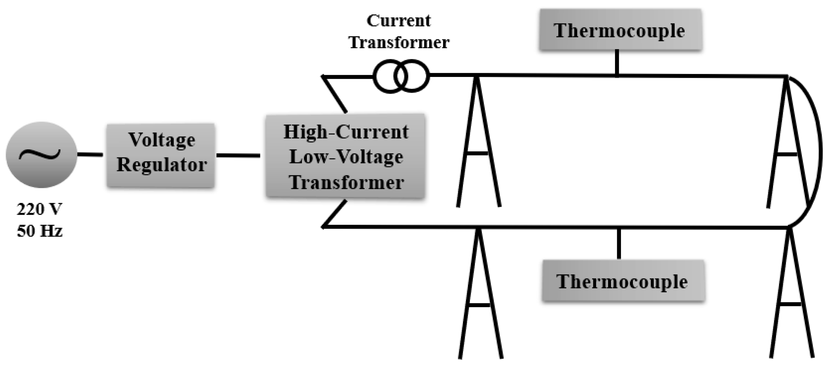
The research conducted during this process has led to the establishment of an experimental platform that accurately simulates the actual operating conditions of ACSR wire. This achievement can be summarized as providing a highly precise and reliable measurement solution. During the measurements, both the AC resistance of the conductor and the steady-state temperature were recorded, allowing for a comparison with theoretical values calculated using the Morgan algorithm [11,12,13]. Following this, a three-dimensional model with a 1:1 diameter wire was developed for finite element simulation to analyze the coupling between electromagnetic and thermal fields. The simulation results were then compared with actual test outcomes to validate the accuracy of the model, thereby enhancing the credibility of these simulation results. In summary, by establishing a robust experimental platform and employing finite element simulations as an auxiliary method—efficiently measuring the AC resistance in ACSR wire while conserving resources—this research methodology and its associated model discussions hold significant value for future transmission line design, optimization, and performance evaluation.

2. Theoretical Calculation of AC Resistance and Simulation Theory Calculation

Although Morgan’s algorithm involves some approximations, the theoretical value of AC resistance is calculated according to EN 60889:1997 [14] and the IEC International standard IEC 61089:1991 [12]. Therefore, Morgan’s algorithm is also used in this paper for theoretical calculation.

At temperature T, the AC resistance per unit length of the conductor can be calculated using Equation (1), as follows:

$$R_{\mathrm{TAC}}=R_{\mathrm{TDC}}+\mathrm{\Delta }{R}_1+\mathrm{\Delta }{R}_2$$

(1)

where $R_{\mathrm{TAC}}$, which represents the DC resistance of the conductor ($R_{\mathrm{TDC}}$) plus two increments, can be calculated. One increment corresponds to the resistance increase resulting from the effects of eddy currents and hysteresis, referred to as $\mathrm{\Delta }{R}_1$, while the other increment accounts for the resistance increase caused by skin effect and proximity effect, denoted as $\mathrm{\Delta }{R}_2$.

Furthermore, it is possible to revise $R_{\mathrm{TDC}}$ more accurately with respect to temperature; this revision exhibits a linear growth trend in relation to an increasing temperature, as shown in Formula (2),

$$R_{\mathrm{TDC}}=R_{20\mathrm{DC}}\left(1-\alpha \mathrm{\Delta }T\right)$$

(2)

where $\mathrm{\Delta }T$ signifies the temperature difference between two temperatures. A reference temperature has been established; the DC resistance at 20 °C is denoted as $R_{20\mathrm{DC}}$. The parameter α denotes the temperature coefficient of resistance at temperature T.

It should also be noted that, when current flows through a conductor, it follows a helical path within its structure. This flow generates an accompanying magnetic field that increases resistive effects, represented by $\mathrm{\Delta }{R}_1$, which are attributed to eddy currents and hysteresis losses. This increase in resistance can be quantified using Formula (3),

$$\mathsf{\Delta }{R}_1=8{\pi }^{2}f{A}_G{\left[\sum _1^m{(-1)}^{m-1}\cdot {\displaystyle \frac{n_m}{l_m}}\right]}^2\mu \tan \delta \times {10}^{-7}/N^2$$

(3)

where $f$ denotes frequency, $A_G$ represents the total cross-sectional area of the steel core, $m$ indicates the number of layers of aluminum stranded wire, and $N$ signifies the total number of aluminum stranded wires within the conductor. Specifically, $n_m$ refers to the quantity of aluminum stranded wires in the $m$-th layer. Additionally, $l_m$ denotes the pitch length of the aluminum conductor in that same layer. Furthermore, $\mu$ represents the overall magnetic permeability of the steel core, while $\tan \delta$ is a physical quantity that measures the energy loss of a material in an alternating magnetic field.

In scenarios where the frequency is sufficiently high, it becomes necessary to account for an additional resistance increment, denoted as $\mathrm{\Delta }{R}_2$, due to both the skin effect and proximity effect. At this juncture, if it simplifies the mathematical model by neglecting electrical conductivity contributions from the steel core itself, it can be treated as a conductive tube for calculation purposes using Formula (4),

$$\mathrm{\Delta }{R}_2=\left[\begin{array}{c}X{(1-\varphi )}^{-1/2}-1\end{array}\right]R_{\mathrm{TDC}}$$

(4)

the factor by which resistance increases due to the skin effect is denoted as $X$, while the factor representing the increase in resistance caused by the proximity effect is indicated as $\varphi$. During estimation processes, should it be determined that the distances between conductors exceed their outer diameter by five times, any influence stemming from proximity effects may be considered as negligible and can, therefore, be disregarded [15].

In summary, according to the basic principle of an AC circuit, the AC resistance of the wire can be approximately calculated by using the above Formulas (1)–(4) based on the theoretical DC resistance.

In addition to the theoretical calculation before the experiment, the theoretical calculation basis of the simulation, the solid heat transfer equation, is used to solve the wire surface temperature after the wire plus AC power in this paper, as follows:

$$\left\{\begin{array}{c}\rho C_{\mathsf{\rho }}u\cdot \nabla T+\nabla \cdot q=Q+Q_{\mathrm{ted}}\\ q=-k\nabla T\end{array}\right.$$

(5)

where $\rho$ represents the mass of a substance per unit volume and velocity $u$ denotes the velocity distribution of a fluid in space, which possesses both magnitude (velocity) and direction. In two-dimensional flow, the velocity vector usually has two components (horizontal and vertical), whereas in three-dimensional flow, it has three components (in the three spatial dimensions); $\nabla \cdot q$ signifies the divergence of heat flux, which reflects changes in the heat flux distribution within a given spatial domain; $Q$ indicates the internal heat sources within the system, referring to heat generated internally; and $Q_{\mathrm{ted}}$ represents external heat sources or terms related to heat exchange. This equation $q=-k\nabla T$ is founded on Fourier’s law of heat conduction, which delineates the relationship between the rate of heat flux and the temperature gradient. The negative sign indicates that thermal energy flows from regions with higher temperatures to those with lower temperatures.

The magnetic field equation is as follows,

$$\left\{\begin{array}{c}\nabla \times H=J\\ B=\nabla \times A\\ J=\sigma E+\mathrm{j}\omega D+J_e\\ E=-j\omega A\end{array}\right.$$

(6)

where $\nabla \times H=J$ is a component of the Ampere–Maxwell law and elucidates the relationship between the curl of the magnetic field strength $H$ and the current density $J$ in the formula $B=\nabla \times A$, where $B$ denotes the magnetic induction strength and $A$ represents the magnetic vector potential. This equation asserts that magnetic induction is equivalent to the curl of the magnetic vector potential. Electrical conductivity $\sigma$ signifies the reciprocal of a material’s capacity to conduct electricity; $E$ indicates both the magnitude and direction of the electric field; an imaginary unit $\mathrm{j}$ is employed to represent phase differences in alternating current; angular frequency $\omega$ characterizes the frequency of alternating current; the electric displacement vector $D$ relates to both electric field strength and material polarization; and the external current density $J_e$ reflects currents supplied by an external power source. $E=-\mathrm{j}\omega A$ illustrates how electric field strength correlates with the magnetic vector potential within an AC circuit. This equation shows that the phase difference between the electric field strength and the magnetic vector potential is 90 degrees, which is a property of the AC electromagnetic field theory. The formula helps the model to understand and calculate the behavior of the electromagnetic field in different media, so as to obtain the AC resistance of different currents [3].

Finally, the boundary condition equation can be established.

$$\left\{\begin{array}{c}\rho C_{\mathrm{p}}u\cdot \nabla T=\nabla \cdot (k\nabla T)+Q_{\mathrm{e}}\\ Q_{\mathrm{e}}=J\cdot E\end{array}\right.$$

(7)

This system of equations delineates the fundamental relationships in heat conduction and electromagnetism, serving to define the boundary conditions for the models presented in this paper. The equation $Q_{\mathrm{e}}=J\cdot E$ relates the electromagnetic heat source term $Q_{\mathrm{e}}$ with the dot product between the current density $J$ and the electric field strength $E$, which characterizes the electrical power density or defines how much heat is produced per unit volume as a current traverses through an electric field.

3. Experimental Research

The experimental conductors utilized in this study were cut to a length of 60 m, and the experiments were conducted in the Civil Engineering and Architecture Laboratory at Southwest University in Chongqing, China. The laboratory dimensions were 61 m in length, 15 m in width, and 13 m in height, thereby meeting the necessary requirements for the experiment. To accurately model the tower structures required for the transmission line, steel frameworks were meticulously constructed at both ends of the laboratory. The reciprocating conductors had to maintain appropriate tension on the overhead lines; this was achieved by manually tightening them with tensioners to ensure that both conductors were suspended at least 1 m above ground level prior to commencing each experiment. Additionally, insulators were installed at connection points between the iron frames and overhead lines to guarantee an effective insulation performance. A laser distance sensor was positioned at the lowest point of the overhead line to measure its minimum sag. To apply varying intensities of excitation to the conductors, a signal generator was employed. Furthermore, an S10 micro-integrator connected to an oscilloscope was utilized for collecting current waveform data. To facilitate simultaneous temperature measurements across multiple points, an eight-channel temperature sensor was deployed for monitoring temperature variations along both overhead lines. This setup allowed for real-time data recording and basic analysis. During thermocouple installation, high-temperature insulating glue was used to secure them at the lowest point of each conductor’s concave section; to minimize data fluctuations and enhance measurement accuracy, four thermocouples were strategically positioned on each conductor at uniform intervals. Specifically, they were placed at the top, bottom, left side, and right side of the conductor to ensure consistent and reliable measurements across multiple points. The detailed specifications of the equipment involved are presented in

Table 1. Introduction of experimental equipment.

Equipment Name	Device Model Number
Laser distance sensor	Keyence LR-TB2000, Osaka, Japan
S10 Micro Integrator	Shanghai PinYan Measurement and Control Technology, Shanghai, China
Eight-channel temperatures of sensor	Victory Instruments VC8801-8, Shenzhen, China
High current generator	Liaoning Lingyuan Precision Instrument Factory, Lingyuan, China
Thermocouple	——
Oscilloscope	——

.

The experimental configuration employed a 220 V, 50 Hz alternating current source. The electrical current flowed through an air circuit breaker and a transformer before reaching a high-current generator, which provided power to the lines. To regulate the magnitude of the output current, the transformer’s output voltage could be adjusted as necessary. During the experiment, the ambient temperature in the laboratory during summer was recorded at 33 °C, with fluctuations maintained within ±2 °C. Furthermore, measures such as temporarily sealing off the air inlets and outlets of the testing hall were implemented to reduce the airflow to nearly zero, thus minimizing any potential interference from ambient temperature on the temperature measurements of the conductors. While it was not feasible to entirely eliminate the influence of surface particles on the experimental outcomes, measures were implemented to minimize this impact. Specifically, prior to conducting the experiments, the surface of the conductor was meticulously smoothed using sandpaper. The overall configuration of the experimental platform is illustrated in Figure 1, while Figure 2 presents the circuit diagram utilized in this research.

All measuring devices utilized in the test were thoroughly calibrated prior to use to ensure the accuracy and reliability of the results obtained. The calibration process adhered strictly to the manufacturer’s specifications, as well as established industry standards, thereby safeguarding the integrity of the collected data. In this study, the following three groups of steel-core aluminum stranded wires with varying specifications were tested: JL/G1A 300/25, JL3/G1A 300/25, and JL/G1A 400/35. Following five different voltage levels of current excitation input, stable temperatures for each conductor along with their corresponding AC resistances were recorded.

4. Simulation Study

In simulation research, the first step is to construct a three-dimensional fundamental model. Initially, the fundamental dimensions and shape of the model are established based on the experimental design, relevant standards [16], and calculations pertaining to the physical wire. Subsequently, sketching tools are employed to accurately create a 3D solid model of the steel-core aluminum wire, with pertinent parameters detailed in

Table 2. Parameters of steel core aluminum strand.

Nominal Section Aluminum/Steel	Calculated Area [mm2]			Number of Single Wire Roots N		Single Wire Diameter [mm]		Diameter [mm]
	Aluminum	Steel	Sum	Aluminum	Steel	Aluminum	Steel	Steel Core	Stranded Wire
JL3/G1A 300/25 *	306	27.1	333	48	7	2.85	2.22	6.66	23.8
JL/G1A 400/35	391	34.4	425	48	7	3.22	2.5	7.50	26.8

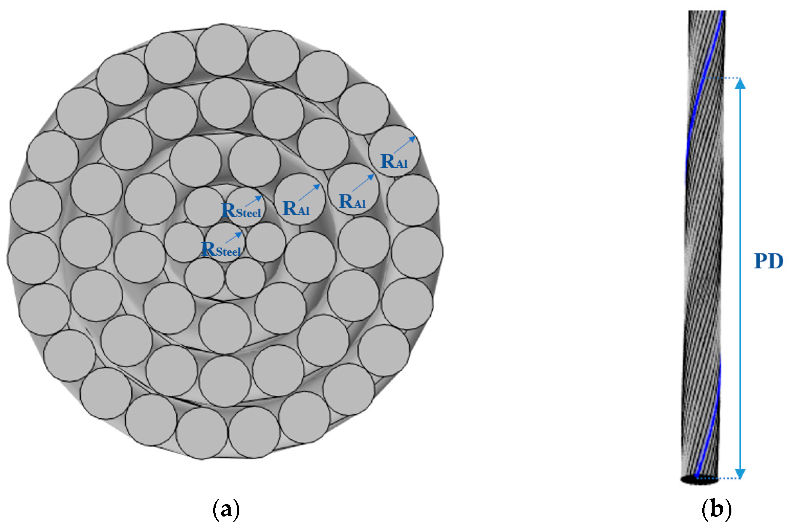
* The parameters of JL/G1A and JL3/1A are consistent, as JL3/1A is exemplified in the table.

. During the modeling process, it is crucial to pay special attention to both the geometric details and physical properties of the model. For instance, intersections between strands must be avoided to ensure that the model accurately reflects its physical behavior under actual working conditions and that the air gaps existing between each strand are minute and almost in close proximity, so they will not notably increase the overall diameter of the stranded wire. The pitch (PD) for JL/G1A 300/25 and JL3/G1A 300/25 is derived from an on-site measurement value of 27 cm, while for JL/G1A 400/35, it measures 30 cm. Finally, visual optimization rendering tools are utilized to enhance the model’s appearance by imparting a metallic sheen, thereby ensuring a high-quality graphic presentation within this article.

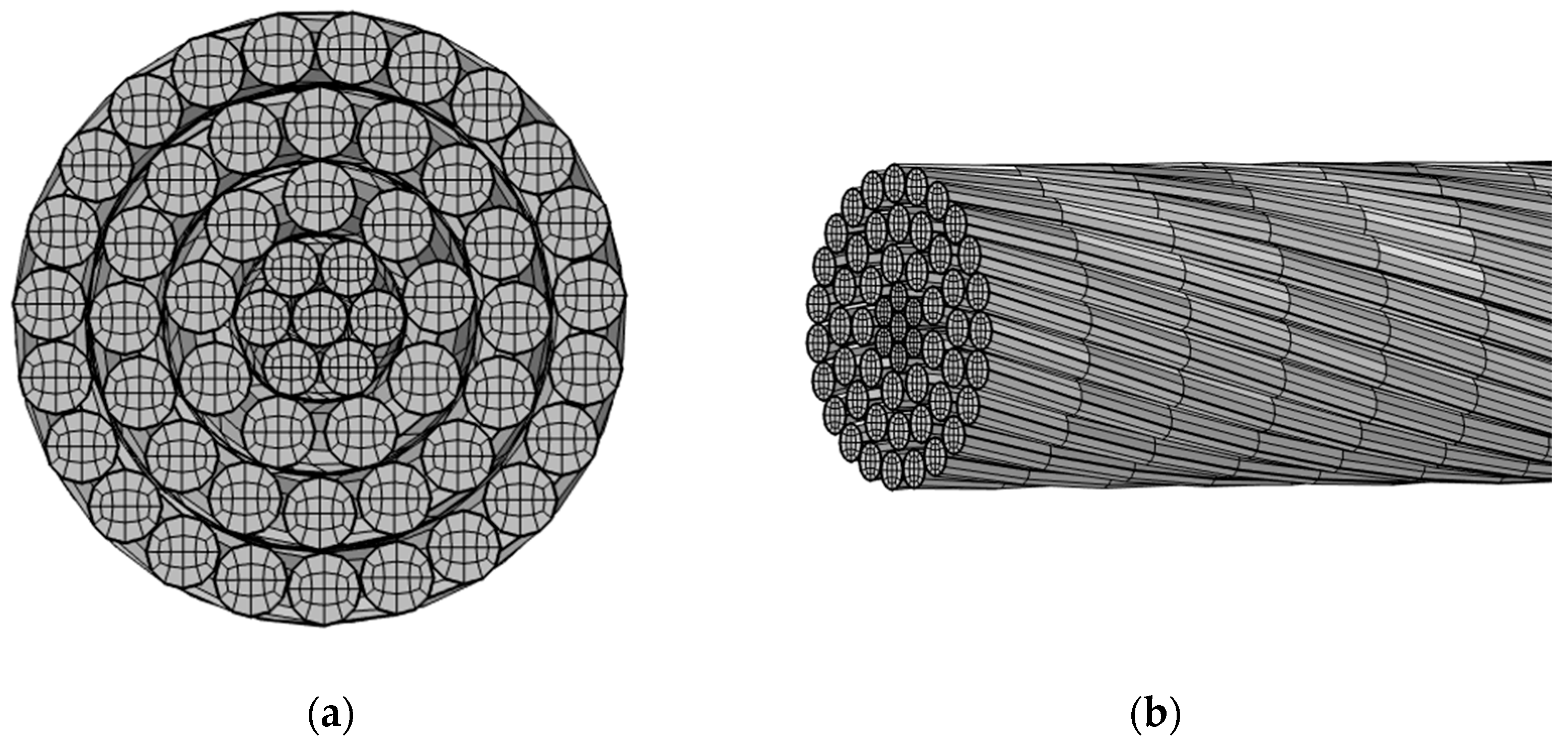
Based on the tabulated data, a three-dimensional model, as depicted in Figure 3, can be constructed.

The process of conducting finite element modeling on the basis of 3D models commences with a distinct definition of the research objective and the relevant physical fields. This study focuses on electromagnetic and thermal fields, aiming to analyze both the frequency domain and steady state of steel-core aluminum wires with specific structures under varying alternating current (AC) conditions. Particular emphasis is placed on examining the AC resistance and temperature variations within these wires. Initially, a three-dimensional model is established, which facilitates the analysis of electric and thermal fields. In the simulation model, a 0.6 m long wire segment is employed to represent a 60 m long conductor, a widely accepted practice in computational modeling. When the current distribution along the conductor exhibits periodic behavior, periodic boundary conditions can be applied to effectively simulate an infinitely long conductor. This method significantly reduces the computational complexity of the model while preserving the accuracy of the physical phenomena. Additionally, by implementing a well-refined mesh, particularly in critical regions such as the wire ends and areas with concentrated current, the model ensures an adequate resolution for precise analysis. The interfaces selected for this analysis encompass “solid-state heat transfer”(ht) within the “AC/DC module”, where the type of heat flux is selected as convective heat flux and the heat transfer coefficient is set at 10 W/(m²·K) [17], “magnetic field”(mf), where the coil current is custom-defined as the variable I_in A and is a periodic function, and “electromagnetic heat”, namely, the coupling of the mf and ht. The interfaces selected for this analysis include “solid-state heat transfer”, “magnetic field”, and “electromagnetic heat” within the “AC/DC module”. Once the type of field is determined, the appropriate boundary conditions and initial conditions are defined. In this finite element simulation’s initial conditions, we consider the following three wire configurations: JL/G1A 300/25, JL3/G1A 300/25, and JL/G1A 400/35. For all configurations, we take into account the nominal cross-sections of aluminum and steel. The relative permeability values are set at 1 for aluminum and 200 for steel. Additionally, constant-pressure heat capacities are specified as follows: aluminum at 900 J/(kg·K) and steel at 475 J/(kg·K). Thermal conductivities are assigned as well; aluminum exhibits a conductivity of 238 W/(m·K), while steel has a conductivity of 44.5 W/(m·K). Both materials have a relative dielectric constant equal to one. Lastly, their densities are noted as follows: aluminum at 2700 kg/m³, while steel is recorded at 7850 kg/m³.

In order to numerically solve partial differential equations, meshing the geometric model is a critical step. Selecting an appropriate mesh density is essential for ensuring both the accuracy and efficiency of the calculations. In this paper, the models employ a free quadrilateral grid (end face with default extremely fine) and utilize a “sweep” technique (number of 60 units) to construct an exceptionally fine mesh that satisfies the computational requirements illustrated in Figure 4. This method of mesh partitioning effectively adapts to complex calculation demands while maintaining the accuracy and reliability of the simulation results. Furthermore, it is crucial to configure solver parameters, including the type of solver (whether direct or iterative) and solver accuracy. Choosing an appropriate solver tailored to specific problems can significantly enhance computational efficiency.

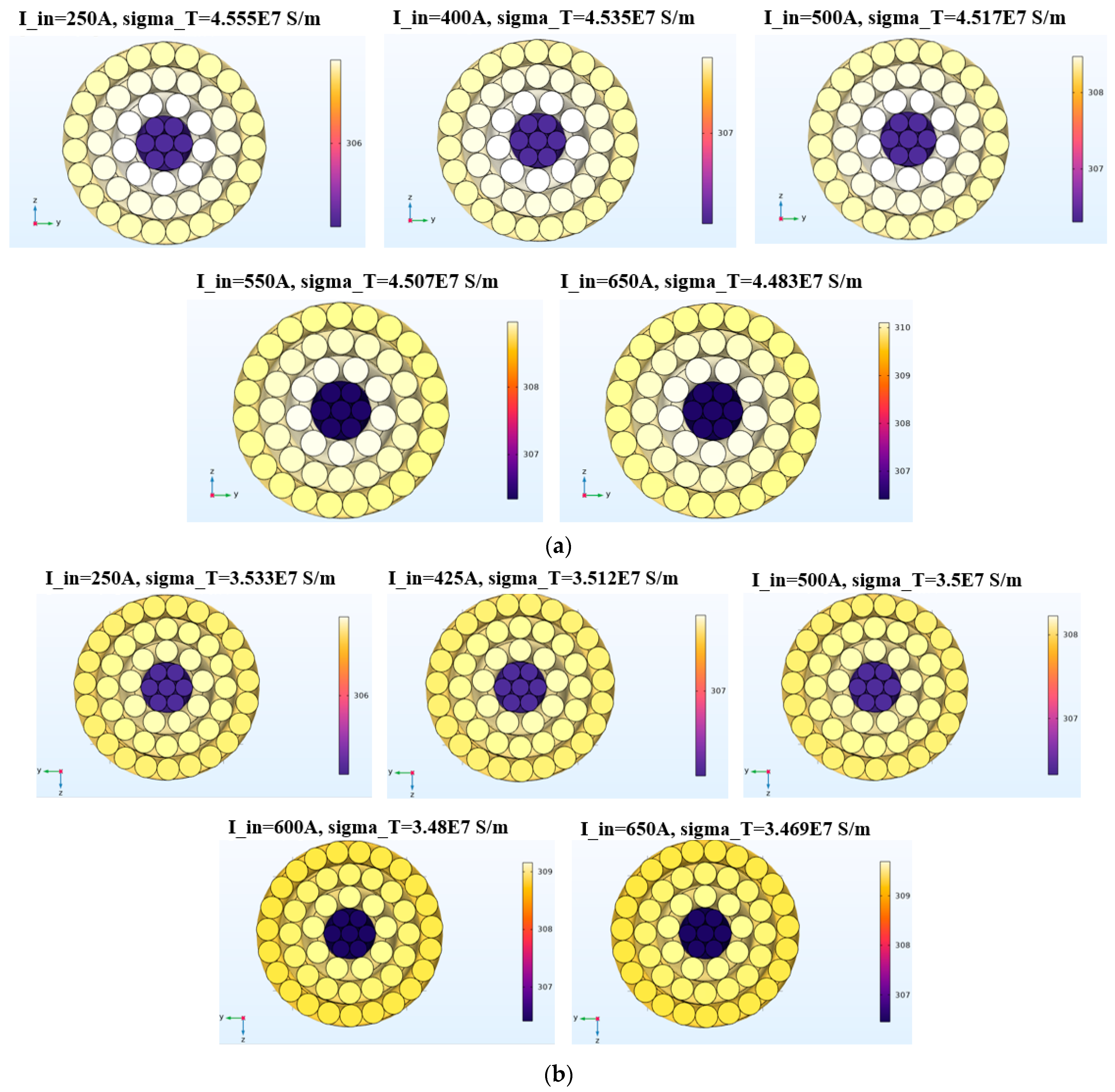
After completing the simulation, the AC resistance values for JL/G1A 300/25, JL3/G1A 300/25, and JL/G1A 400/35 are determined to be 0.1017 Ω/km, 0.1074 Ω/km, and 0.1013 Ω/km, respectively. These values are based on the weighted average temperature corresponding to the input AC current levels. To enhance alignment with real-world conditions, it is essential to incorporate temperature-dependent resistivity changes into the model under development as temperatures increase. In the section of the conductor material aluminum, the electrical conductivity will no longer be a constant, but rather transform into a custom-defined variable, sigma_T, with the unit of S/m. The quantity revised in accordance with temperature variations is incorporated into the material parameters. The revised values are presented in

Table 3. The DC resistivity, along with the temperature coefficient of resistance (20 °C).

Type of Aluminum Wire	DC Resistivity at 20 °C [Ω was/m (% IACS)]	1/ρ at 20 °C [S/m]	Temperature Coefficient of Resistance at 20 °C [1/°C]
L	0.028 264	35,380,000.00	0.004 03
L3	0.027 586	36,250,000.00	0.004 13

.

For each type of wire, the theoretical value of AC resistance is calculated based on the necessary parameters collected, utilizing the aforementioned Formula (2). This approach allows for a comprehensive analysis and optimization of parameter sensitivity, informed by preliminary conductivity results that vary with temperature. The increase in temperature resulting from different currents will influence the resistivity values, thereby aligning more closely with real-world conditions.

It is important to note that a distinct image for the JL/G1A 300/25 model is not provided separately in Figure 5, as its variation trend can be sufficiently referenced through the JL3/G1A 300/25 model. The calculation of the alternating current resistance of conductors is essential for the design and performance evaluation of transmission circuits. Consequently, this paper presents an experimental design aimed at measuring the alternating current resistance of various conductors. However, it is important to note that this experiment is labor-intensive and resource- and time-consuming. Therefore, an effort is made to develop a simulation model that can effectively estimate the alternating current resistance of conductors, thereby facilitating future evaluations, applications, and designs involving ACSR wire.

Firstly, this study calculates the theoretical values for the alternating current resistance of three types of conductors based on Formula (2). These theoretical values serve as benchmarks against which the results obtained from the simulation model with a variable resistivity are compared. If the simulation results for each type of conductor fall within a credible error range relative to their corresponding theoretical calculations upon the completion of the simulation process, it will validate the applicability of the model. The discrepancy between these two sets of values is quantified using Formula (8),

$$\mathrm{Error}={\displaystyle \frac{\mathrm{Standard}\mathrm{Deviation}}{\mathrm{Mean}}}\times 100\%$$

(8)

where the standard deviation and mean values are both obtained from theoretical calculations as well as model simulation results, which are presented in

Table 4. Comparison between theoretical calculation and simulation calculation of AC resistance.

Cable Models	Applied Current [A]	Theoretical Calculation of AC Resistivity [Ω/km]	Simulation Calculation of AC Resistivity [Ω/km]	Error Rate %
JL/G1A-300/25	200	0.10249	0.10779	3.567%
	350	0.10683	0.10842	1.050%
	425	0.11060	0.10885	1.130%
	500	0.11385	0.10940	2.813%
	550	0.11802	0.10981	5.101%
JL3/G1A-300/25	250	0.10084	0.11249	7.725%
	400	0.10473	0.11298	5.356%
	500	0.10794	0.11343	3.506%
	550	0.11184	0.11368	1.153%
	650	0.11644	0.11428	1.326%
JL/G1A-400/35	250	0.09060	0.09459	3.046%
	425	0.09377	0.09514	1.028%
	500	0.09682	0.09547	0.995%
	600	0.09985	0.09601	2.767%
	650	0.10284	0.09631	4.639%

.

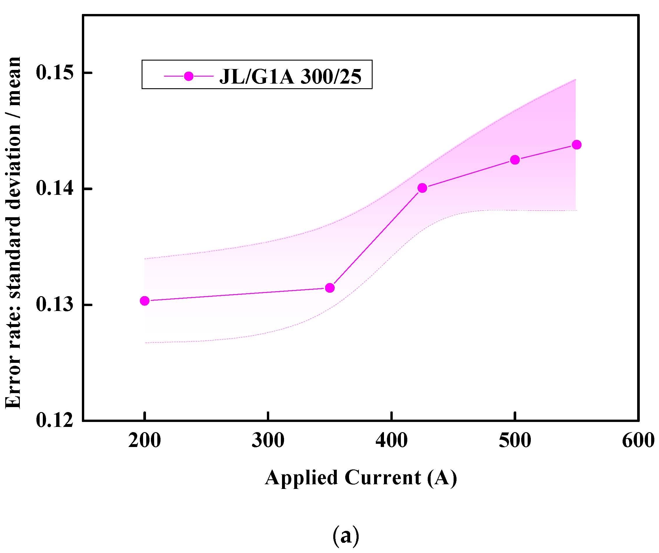
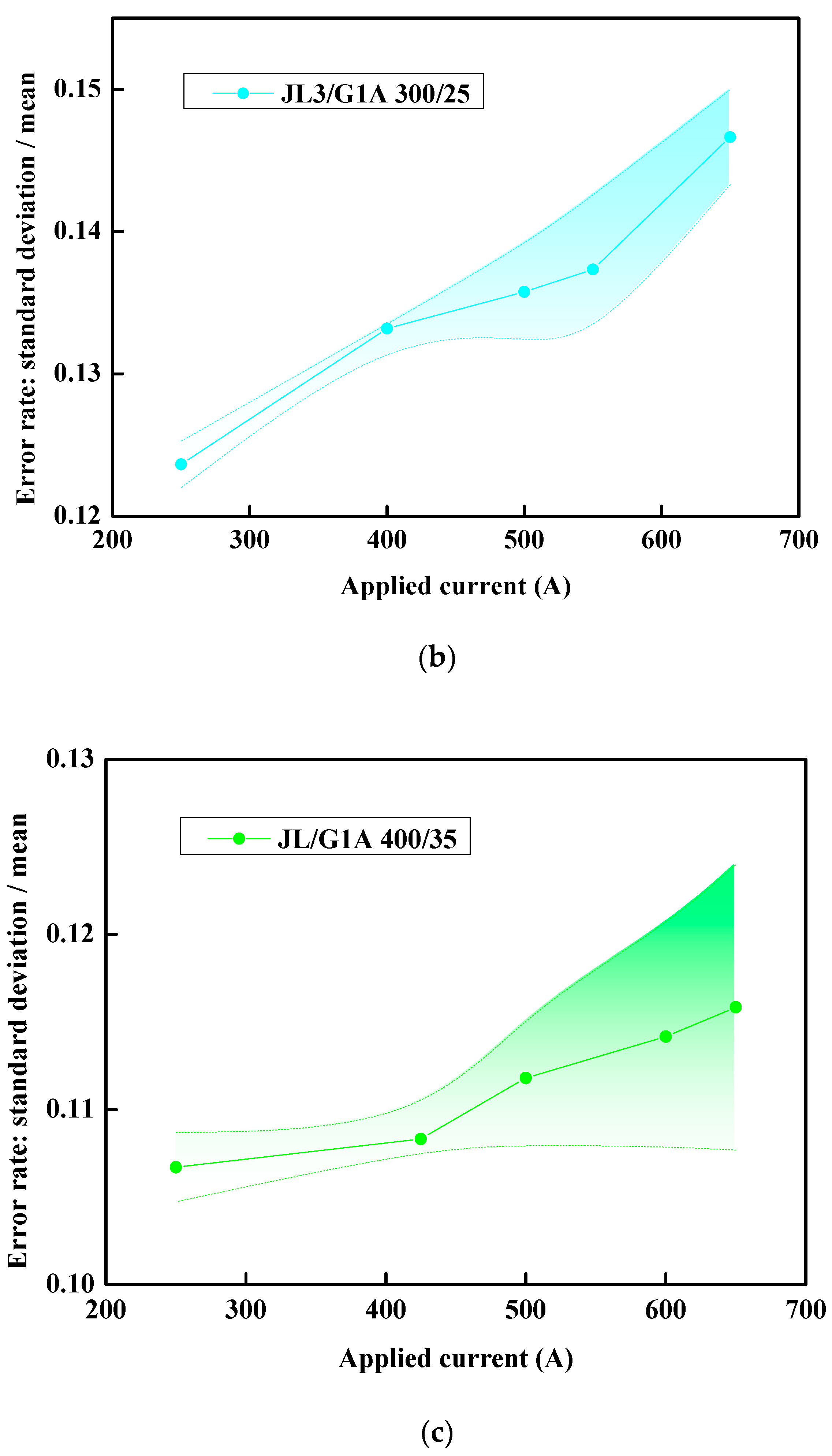
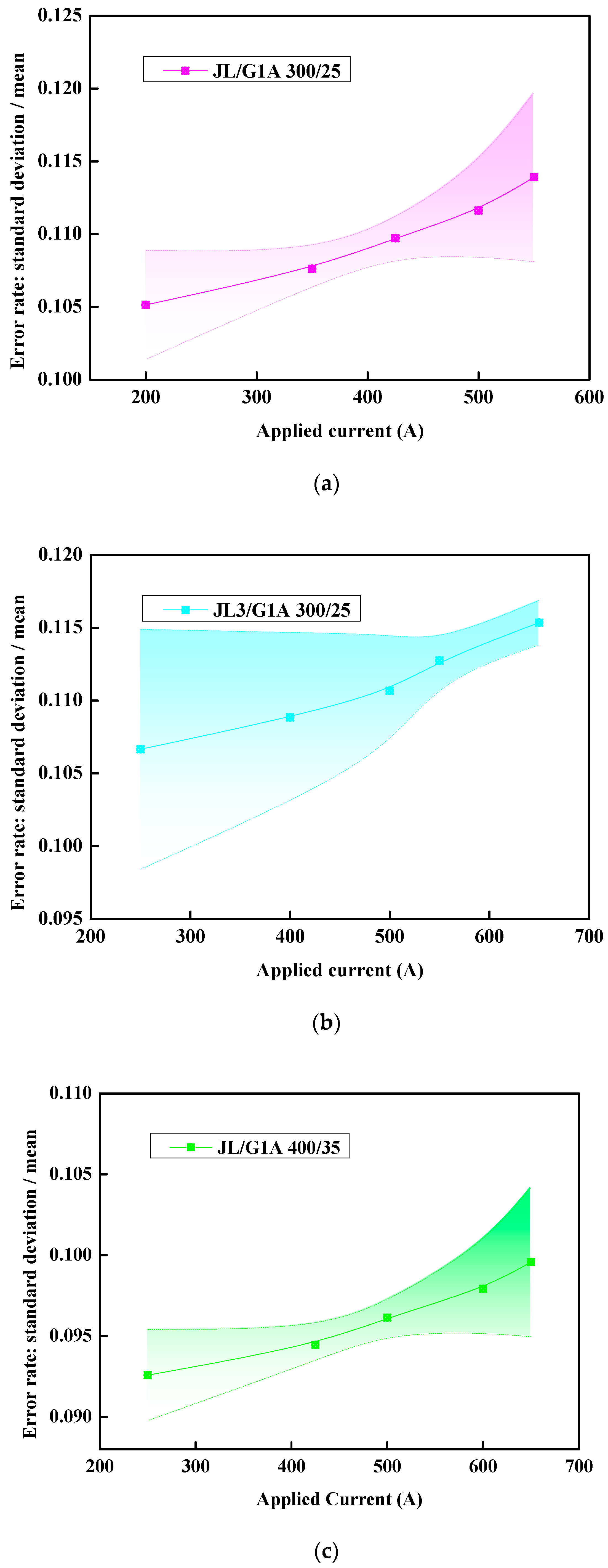
For each type of wire, the error rate values presented in the final row of Table 4 indicate that the discrepancy between the calculated and simulated values falls within an acceptable range, specifically less than 10% [18,19]. This suggests that the model can be effectively utilized in subsequent experimental measurements to provide valuable assistance. To enhance the accuracy and reliability of the simulation model, an error band graph illustrating both the mean and standard deviation—depicted in Figure 6—can also be constructed to demonstrate the extent of data uncertainty.

The graph presented above visually illustrates the potential error or uncertainty associated with each data point. The fluctuations in the sample data are represented by the standard deviation, while the uncertainty of the sample mean is also quantified by this measure. This approach allows for a clear observation of the deviations between the simulation results and theoretical values. These discrepancies primarily arise from the following two sources: first, the uncertainties inherent in the material parameters, and second, the approximations made within the model itself. Nevertheless, error analysis indicates that these deviations remain within a controllable range, thereby reinforcing the feasibility of employing the simulation model to estimate AC resistance.

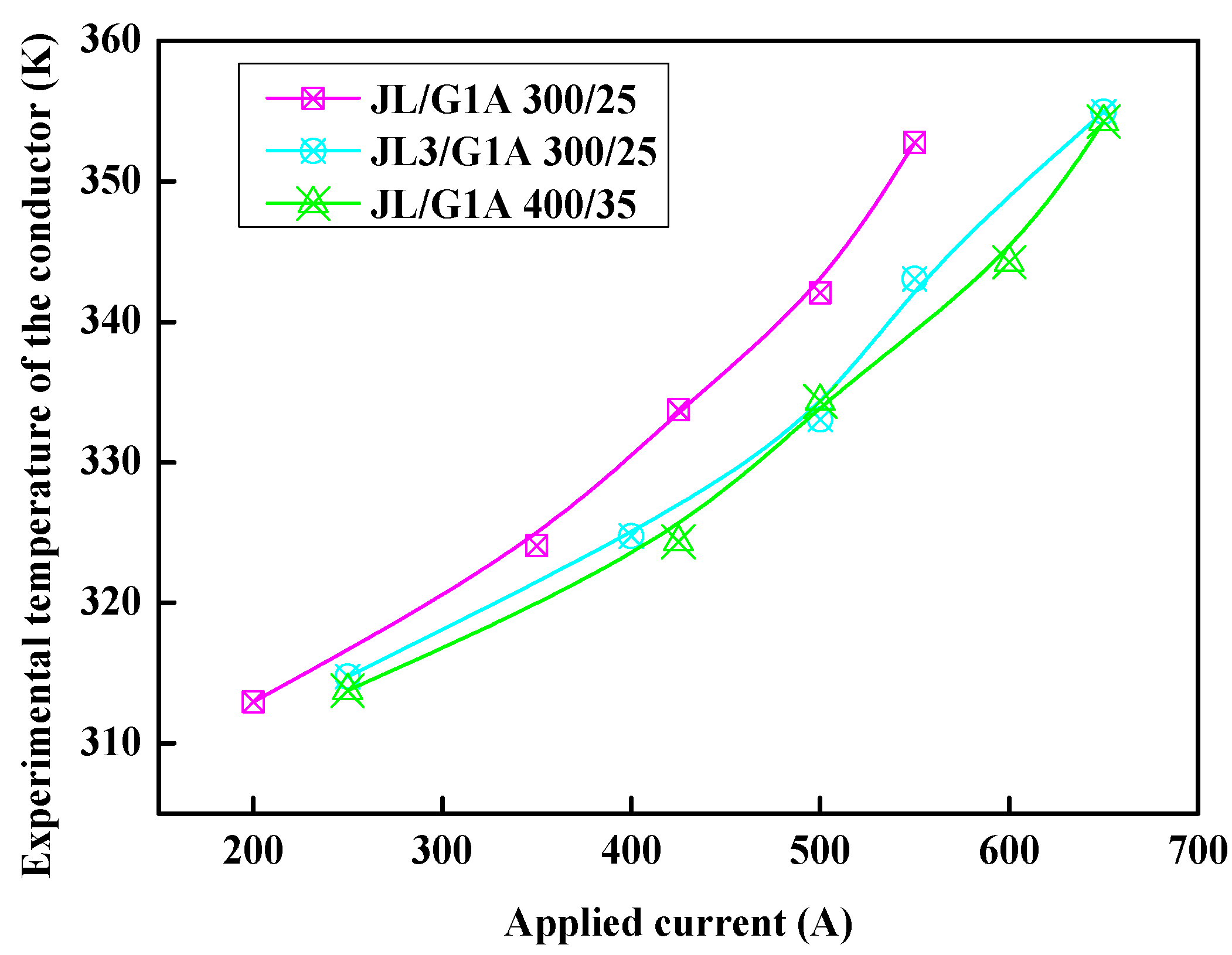
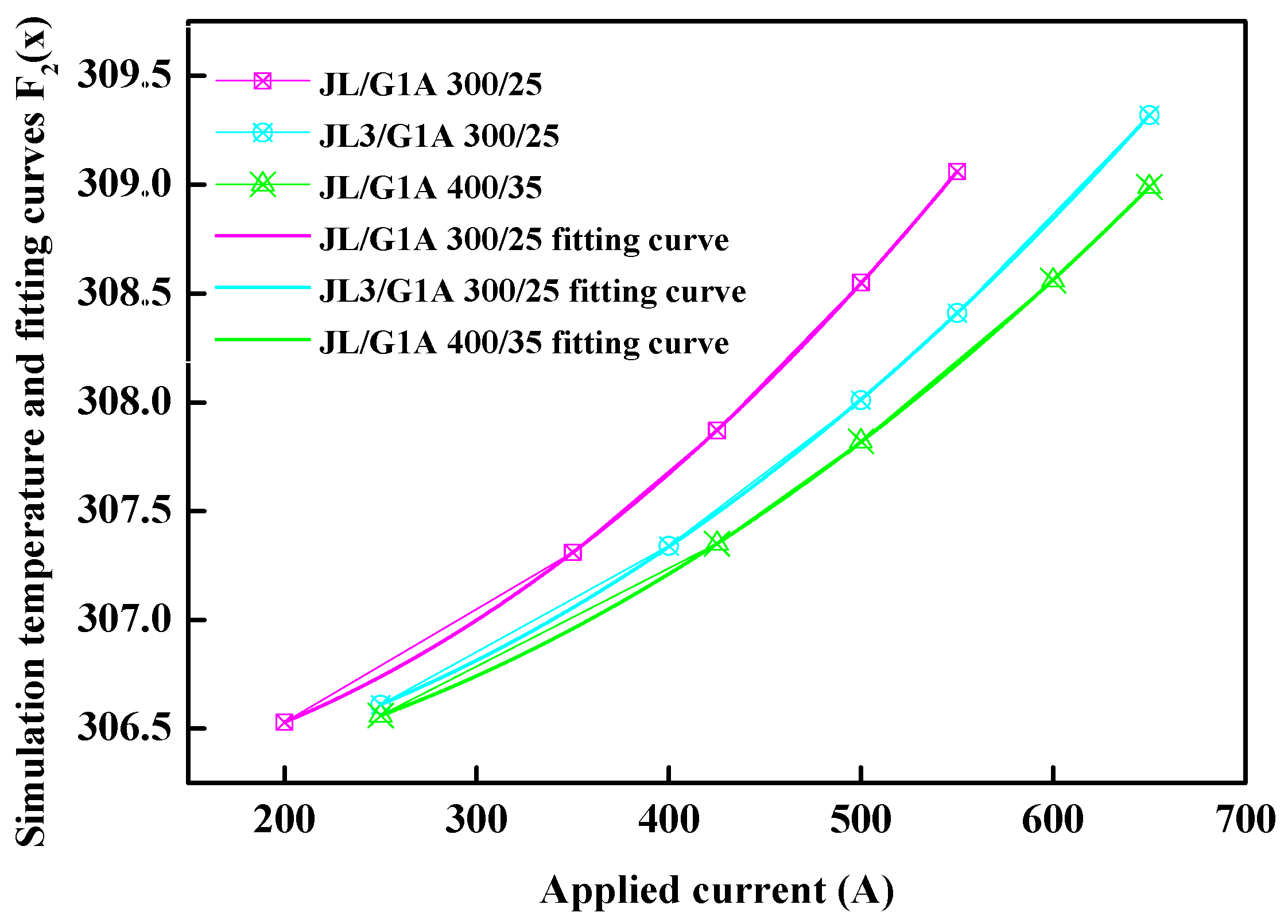
Then, utilizing the experimental platform established previously, the test sampled the AC resistivity of three types of conductors and obtained stable temperature values under varying current intensities to construct the measured temperature rise curves, as illustrated in Figure 7. Concurrently, the simulation model also provided temperature curves derived from simulations conducted at different current intensities, as depicted in Figure 8. At this juncture, a notable discrepancy was observed between the simulation results of the model and the actual measured values. This divergence may be attributed to several factors, including uncertainties related to the material properties; for instance, the simulation employed theoretical parameters without accounting for the actual material properties of the cables used in practice. In contrast, the measured conductors were operational units that likely exhibited certain dirt or oxide layers on their surfaces. Additionally, there was an incomplete alignment of boundary conditions; specifically, this model only considered solid heat transfer coupled with magnetic fields while neglecting heat dissipation conditions and other relevant settings. Furthermore, physical phenomena that were not thoroughly examined within the model could have contributed to these differences—such as variations in the thermal cycles experienced by actual conductors during operation.

However, considering that the temperature curves obtained from both the experiment and simulation exhibit an identical upward trend, this paper employs a method of temperature function approximation to minimize the discrepancy between the actual test temperature values and the simulated temperature values. All unknown parameters are treated as system errors, allowing for a reduction in the gap between the measured and simulated values to optimize the model parameters. The adjusted temperature values are then utilized to estimate the AC resistance, thereby verifying whether the error between the simulation results and experimental measurements falls within an acceptable range. The specific methodology involves fitting both an actual measurement temperature curve ${\mathrm{F}}_1(x)$ and simulated temperature curve ${\mathrm{F}}_2(x)$(identified quadratic functions). Following this, an error function curve $\mathrm{F}(x)$ is derived from these two functions. This error function curve serves to adjust the simulation results; specifically, it reduces temperature discrepancies based on the steady-state temperature rise curve generated by the simulations. Consequently, the final AC resistance values are calculated using this refined model.

From Figure 8, the temperature fitting curves for the three models following the simulation can be observed, as detailed below,

• JL/G1A 300/25: ${\mathrm{F}}_2(x)=306.20-3.88\times {10}^{-4}x+1.02\times {10}^{-5}{x}^2$,
• JL3/G1A 300/25: ${\mathrm{F}}_2(x)=306.17-1.90\times {10}^{-4}x+7.73\times {10}^{-6}{x}^2$,
• JL/G1A 400/35: ${\mathrm{F}}_2(x)=306.17-1.53\times {10}^{-4}x+6.91\times {10}^{-6}{x}^2$.

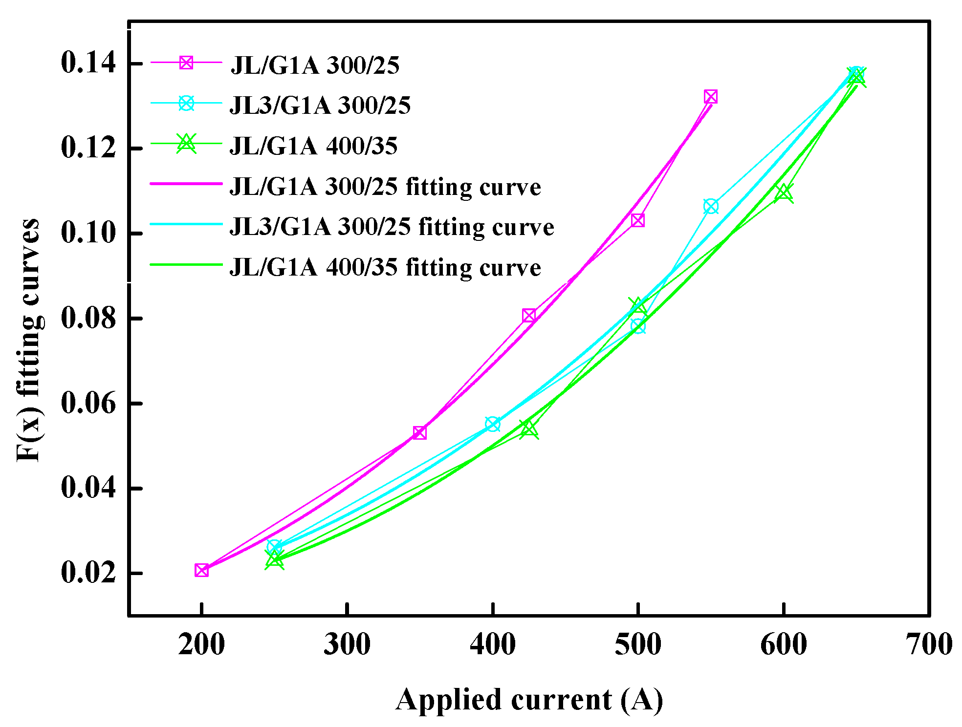
As mentioned above, the experimental temperature curve function is defined as ${\mathrm{F}}_1(x)$, while the simulation temperature curve function is represented by ${\mathrm{F}}_2(x)$. By comparing these two values, we can derive the error function $\mathrm{F}(x)={\displaystyle \frac{{\mathrm{F}}_1(x)}{{\mathrm{F}}_2(x)}}$. The data processing results are presented as follows,

$$\ln {\displaystyle \frac{{\mathrm{F}}_1(x)}{{\mathrm{F}}_2(x)}}=\ln {\mathrm{F}}_1(x)-\ln {\mathrm{F}}_2(x)=\mathrm{F}(x),$$

(9)

$$\ln {\mathrm{F}}_1(x)=\ln {\mathrm{F}}_2(x)+\mathrm{F}(x)$$

(10)

$$e^{\ln {\mathrm{F}}_1(x)}=e^{\ln {\mathrm{F}}_2(x)+\mathrm{F}(x)}=e^{\ln {\mathrm{F}}_2(x)}{e}^{\mathrm{F}(x)}$$

(11)

$${\mathrm{F}}_1(x)={\mathrm{F}}_2(x)e^{\mathrm{F}(x)}$$

(12)

The stabilized temperature was subsequently plotted, as illustrated in Figure 9. Sim-ultaneously, the ascending curve was fitted using a quadratic term.

After fitting, the error function expression can be found as follows,

• JL/G1A 300/25: $\mathrm{F}(x)=0.01-4.08\times {10}^{-5}x+4.71\times {10}^{-7}{x}^2$,
• JL3/G1A 300/25: $\mathrm{F}(x)=0.01-3.80\times {10}^{-5}x+3.57\times {10}^{-7}{x}^2$,
• JL/G1A 400/35: $\mathrm{F}(x)=0.02-7.55\times {10}^{-5}x+3.94\times {10}^{-7}{x}^2$.

As long as any current intensity excitation is applied during the simulation process and a stable temperature value is achieved, the corresponding stable experimental temperature can be determined using the temperature function correction from Formula (12). Subsequently, this experimental temperature value can be substituted into Formula (2) to adjust the fundamental DC resistance parameter values of the simulation model. This adjustment allows for the calculation of the final AC resistance magnitude, which can be utilized to approximate the actual measured values of the conductors and will also be applied to other estimations.

The final AC resistance obtained after the revision to align with the measured temperature was compared against the measured values, and an error analysis chart was generated. It is evident that this also satisfies the error requirements. For further details, please refer to

Table 5. Comparison of actual test values and revised simulated calculated AC resistances.

Cable Models	Applied Current [A]	Actual Test Values of AC Resistivity [Ω/km]	Revised Simulation Calculation of AC Resistivity [Ω/km]	Error Rate %
JL/G1A-300/25	200	0.1329	0.12779	2.77%
	350	0.1345	0.12842	3.27%
	425	0.1413	0.13885	1.24%
	500	0.1456	0.13940	3.07%
	550	0.1478	0.13981	3.93%
JL3/G1A-300/25	250	0.1248	0.12249	1.33%
	400	0.1334	0.13298	0.22%
	500	0.1381	0.13342	2.44%
	550	0.1410	0.13367	3.77%
	650	0.1490	0.14428	2.28%
JL/G1A-400/35	250	0.1053	0.10810	1.86%
	425	0.1079	0.10874	0.55%
	500	0.1145	0.10910	3.42%
	600	0.1186	0.10973	5.49%
	650	0.1216	0.11007	7.04%

and Figure 10.

By implementing a temperature approximation strategy, the simulation model can be optimized to a certain extent, thereby aligning its results more closely with the actual measured values. This process not only enhances the accuracy of the model, but also improves its feasibility for practical engineering applications. Although this model is not universally applicable to all overhead conductors, it proves effective for various types and models of ACSR wire. Consequently, this approach can mitigate the need for extensive conductor replacements during actual measurements, thus saving the human resources, time, and financial costs associated with experimental procedures. However, future work must focus on further exploring additional factors that may influence the accuracy of the simulation model and continue optimizing it to enhance its predictive capabilities.

5. Discussion

In the course of the theoretical calculations and finite element simulation verification of the AC resistance value of the wire, several significant findings and conclusions have emerged:

(1)

The revised temperature parameter model closely aligns with the estimated values, indicating that the model can more accurately predict the resistance characteristics of the wire when accounting for temperature variations. Temperature changes directly influence material resistivity; specifically, as the temperature increases, the electrical conductivity of most metals decreases, while the resistivity correspondingly rises.

(2)

The parameter model adjusted according to actual temperature measurements also approximates the measured values well, demonstrating that the validity of the simulation model has been confirmed in practical applications. This comparison enhances the understanding of the model’s performance under varying conditions and provides a foundation for future design enhancements.

(3)

Although the model values are in close proximity to the measured ones, certain discrepancies remain. These errors may arise from factors that were not fully accounted for, such as heat dissipation conditions, thermal cycling, and the wear and oxidation of wires following usage. While the skin effect is not pronounced at 50 Hz in this study, it cannot be dismissed as a potential source of error. Additionally, wire contamination may alter the surface characteristics of the conductor, thereby affecting both the current flow and heat distribution.

6. Conclusions

This paper presents a theoretical calculation and simulation of the AC resistance values for three types of identical conductors. The findings indicate that the simulation model, when combined with the function revision method, can effectively predict and estimate the AC resistance series of conductors. This discovery holds significant implications for conductor design and circuit performance evaluation, as it offers a reliable simulation tool to forecast and optimize conductor performance.

However, it is important to note that the current model exhibits certain limitations, such as a reliance on function revision. To enhance both the accuracy and direct applicability of the simulation model in future applications, more complex models along with advanced simulation parameters and environmental coupling may be required. Such improvements would substantially augment the predictive capabilities of the model.