Control Parameters of a Wall Heating and Cooling Module with Heat Pipes—An Experimental Study

Abstract

Heat pipes filled with a thermodynamic medium are energy-saving and stable heat exchangers that have been used for years in various fields of science and technology, including building heating and cooling installations. This article presents the results of research on the energy efficiency of wall-mounted concrete heating and cooling modules with heat pipes, which can be a structural element of external and internal walls of buildings for various purposes. A series of measurement tests were performed, which allowed the determination of how the thermal power and control parameters of the module (amplification factor and time constants) change under operating conditions. A first- and second-order inertial model was used to describe the control properties of the module. The measurements were performed in heating and cooling mode for three different values of supply water flow, both when increasing the supply temperature and when decreasing it. Based on the results of the measurements, calculations and analysis, it was found that the thermal power and control parameters of the module change significantly; these changes result from both the design features of the module (the type of thermodynamic medium in the heat pipe and the technical aspects of the execution and assembly of the connections between the collector and the heat pipe) and the operating conditions (the value of the direction of temperature change and the flow of the supply water). It was shown that the supply temperature has a much greater impact on the values of the module’s control parameters than the flow rate of the supply water. The tested module is characterized by slow changes in temperature on its surface (high values of time constants). The time of stabilization of the temperature on the module’s surface, after step forcing, is 8–10 h. This can cause greater fluctuations in the indoor air temperature, lower thermal comfort in the room and lower energy efficiency of the process. These issues can be prevented by using complex algorithms for thermal comfort control, which in turn increase the cost of the control system.

1. Introduction

One of the most important goals for preventing climate change is reducing carbon dioxide emissions into the atmosphere. This can be achieved by the extensive use of energy from renewable sources and so-called waste energy. Unfortunately, the carriers of this energy used in the construction industry are characterized by low parameters. On the other hand, building sector is the second, after transport, consumer of energy needed to maintain thermal comfort and sanitary needs of users, therefore, the type and amount of energy used in this sector is of significant importance to the overall energy balance and impact on the environment. With the progress of civilization, building users expect increasingly better living conditions, including higher thermal comfort, which does not favor the reduction of energy consumption. In temperate countries, where there is a need to heat rooms in winter and cool them in summer, the demand for energy is increasing. The solution is to use energy obtained from renewable sources or to use waste energy. One of the solutions for enabling the use of energy contained in low-parameter carriers in building heating installations is so-called surface exchanger heating. Surface heating uses large surface exchangers, usually integrated with the room partitions [1,2,3]. Their surface temperature is relatively low, which is a beneficial factor because it ensures a more even temperature distribution in the room and improves the thermal comfort of users, compared to traditional convection exchangers [4,5]. Due to their large surfaces, surface exchangers can be used to supply and receive heat, and thus to heat and cool the room. Heat exchange between the exchanger and the room and its users takes place mainly by radiation, which increases the efficiency of heat release by users in the summer due to the light clothes worn during this period [6].

So far, water has been used in surface heat exchangers as a heat-distributing or heat-dissipating medium. Recently, heat pipe exchangers have been gaining popularity [7,8]. Like most heat exchangers, they transfer heat from a higher-temperature environment to a lower-temperature environment. Only the principle of heat exchange is different. In water heat exchangers, water flows in coils immersed in the radiator material. In heat pipe exchangers, an intermediate phase-change thermodynamic medium is used, which extracts heat from water and transfers it to the exchanger material. Heat exchange occurs by cyclic change of state, from liquid to gas and from gas to liquid [8,9].

The basic advantages of this solution using heat pipes are as follows:

-

fast heat transfer, resulting mainly from the relatively high speed of gas movement under the influence of the temperature difference (or gravitational flow of liquid);

-

no moving parts and no additional energy consumption and costs to force the movement of gas or liquid (the thermodynamic medium moves freely);

-

lower probability of failure due to the closed space of the heat pipes;

-

wide range of operating temperatures of the pipe, resulting from the possibility of using various thermodynamic mediums and their mixtures with different structures;

-

a properly selected thermodynamic medium can transfer heat in both directions, i.e., it can transfer heat or receive it from rooms without changing the structure of the exchanger.

The main disadvantage of heat pipe exchangers is the short distance of heat transfer using a thermodynamic medium, especially when the heat pipes are horizontal, in which case there is no gravitational support for the movement of the liquid, or when heat is transferred from top to bottom, in which case the viscous and gravitational forces have opposite signs.

Heat pipe technologies have been successfully used for many years in various fields of science and technology [8,10,11]. The main sector of application is the recovery of high-temperature, medium-temperature and low-temperature heat [12,13,14]. Heat pipes are used, among other uses, in the collection of heat from electronic systems and photovoltaic panels [15], and of waste heat from technological processes [16,17]. The construction of the exchanger itself can take various forms—from round pipes placed directly in the medium to which they transfer heat [18,19], to plate exchangers [20]. Heat pipes can be mounted both vertically and horizontally [21], as single pipes or connected loops [9]. The element that affects the efficiency of the solution is the appropriate selection of the thermodynamic medium, the phase change temperature of which should be adjusted to the temperature occurring in the system under consideration. Various substances are used as thermodynamic media, such as ammonia, acetone, methanol, freons [22] and nanoliquids [23,24].

The wide area of application, various thermodynamic factors and various heat pipe structures mean that many classifications of heat pipes can be given, adopting different classification criteria. One of the most general is the classification that takes into account the essence of heat pipe operation, from the simplest thermosyphon to the most complex nanotubes. According to this criterion, seven groups of heat pipes were distinguished:

• Thermosyphon systems (ThSs) with single-phase refrigerant work on the principle of heat rising [7,8].
• Conventional Heat Pipes (CHPs), which are a self-contained structure and operate within a two-phase flow regime as evaporation–condensation devices for transferring heat [7,8].
• Pulsating Heat Pipes (PHPs), which differ from Conventional Heat Pipes in that their capillary tubes contain vapor bubbles of the working medium [7,9].
• Loop Heat Pipes (LHPs) and Capillary Pumped Loops (CPLs), which are two-phase heat transfer devices that operate in a feedback loop [8,9].
• Rotating and revolving Heat Pipes, in which the condensate is returned to the evaporator through centrifugal force, and no capillary wicks are required [8].
• Micro Heat Pipes (MHPs), which differ from Conventional Heat Pipes in that they are much smaller. They do not contain a wick structure to assist the return of the condensate to the evaporator section; instead, they use capillary forces. They are used in computer technology [8,9].

Each of the above-mentioned heat pipe cases can be described using different mathematical models. The choice of model depends on the heat pipe structure and the expected accuracy of the model. In practice, three models are used, differing in their degree of complexity and calculation time, but above all, in the accuracy of their obtained results. These are as follows:

• Transient lumped model—the simplest and least accurate.
• One-dimensional transient continuum model.
• Two-dimensional transient continuum model—the most complex, but also the most accurate.

In the heat exchange model prepared in the construction module, the use of one- or two-dimensional continuous models is planned. In the experimental studies, the first- and second-order transient lumped model was used (lumped model).

Examples of heat pipe applications for HVAC systems include a radiant heater made of heat pipes connected to an air heat pump [25], heat recovery from ventilation air [26], exhaust gasses from heat sources [27] and the use of heat pipes as a heating element mounted in the wall of a room [28,29] or an entire building [30]. However, there is a lack of research and publications on the behavior of heat pipe wall exchangers operating in heating and cooling mode within the same thermodynamic medium. Analyzed issues of bidirectional heat exchange during energy storage using a heat pipe and PCM elements [31,32,33] are not the same as heating and cooling exchanges in building rooms (because of the quite different condition of their exploitation).

In climate zones where both heating and cooling are required, heat exchangers that can operate in both heating and cooling modes are desirable, without changing the thermodynamic medium in the tubes. It would be best if these heat exchangers were integrated with the building structure. These are the so-called heating and cooling building modules. Such modules can be manufactured as prefabricated elements and then assembled in the building structure on the construction site. This allows for shorter construction times and lower housing costs, which is of significant importance in the country’s economy.

An important feature of heat exchangers is their heat power, which needs a flexible and wide range of change. A simple, fast and wide range of power change is of particular importance in the case of exchangers operating in systems requiring quick adjustment of power to meet current needs. This applies in particular to heated or cooled rooms. Control systems that adjust the exchanger’s power to current needs must be properly designed, manufactured and programmed so as not to generate additional energy losses when adjusting the exchanger’s power to current needs. In order to create such software, knowledge of the heat exchange process in the exchanger is required, i.e., knowledge of the thermal properties of the heating and cooling module as the control object. The thermal properties of the module, like any exchanger, depend on many factors. They can be divided into two groups. The first are factors related to the construction of the module, over which the user has no influence. These include the following:

-

the construction of the heat exchanger (geometric dimensions, filling building material);

-

the number and location of heat pipes in the exchanger material;

-

the type and physical properties of the thermodynamic medium filling the pipe;

-

the shape of the internal surface of the heat pipe;

-

the method of placing the ribs in the building material (in the case of reinforced concrete modules).

The second group consists of operating factors which, at least to some extent, can be shaped by the user. This group includes the following:

-

the position of the exchanger (its inclination in relation to the horizontal surface);

-

the method and range of change of the exchanger power;

-

the method and range of change of the temperature and flow of the supply water.

The aim of the conducted research was therefore to investigate and analyze changes in parameters characterizing the thermal static and dynamic properties of the building’s heating and cooling module as a control object, which can be used for programming and setting the control system. This article presents the experimental results and the conclusions in the following scope:

-

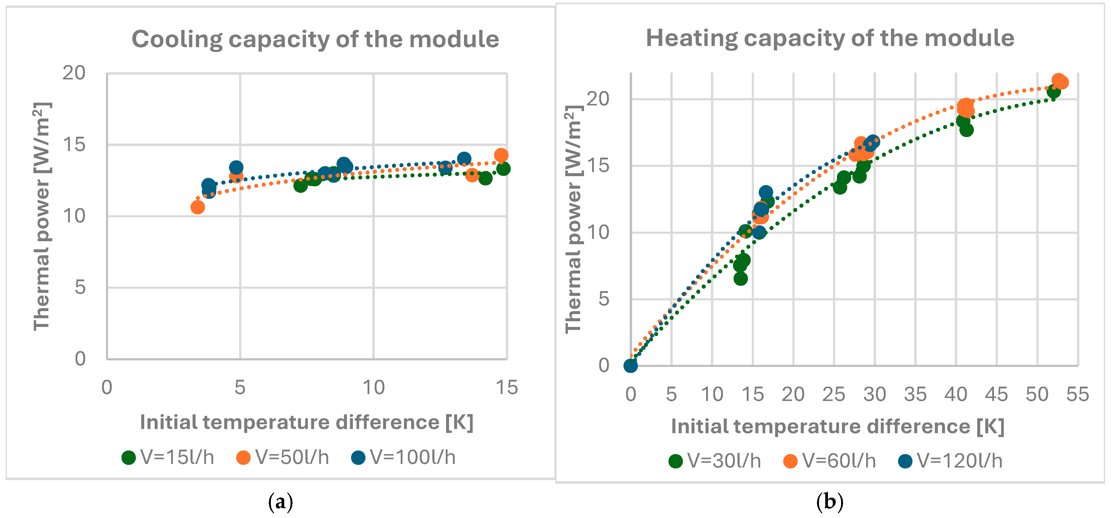
changes in the thermal power in cooling mode and in heating mode when changing the flow and temperature of the supply water; these results can be used to select heating and cooling modules in the designed room;

-

changes in the gain coefficients and time constants of the inertial models, describing the static and dynamic properties of the module as a control object when changing its power during operation; these results will be helpful for correct programming and setting of the module’s power control system for maintaining thermal comfort in the room. The adopted inertial models are most often used to identify the dynamics of thermal objects [34,35,36].

Moreover, the influence of operating factors on the changes in the values of the amplification coefficients and time constants of the inertial substitute models was analyzed in detail; the results of the analysis can be used in the independent design of building module constructions using heat pipes.

To sum up, the choice of the topic of wall heating and cooling modules using heat pipes results from the search for innovative and effective installation solutions for construction that allow for obtaining a reliable and economical method of heating and cooling buildings. The beneficial energy properties and high thermal comfort of water surface systems lead to the search for new solutions/modifications of classic systems that will allow for obtaining similar thermal properties, while reducing or eliminating unfavorable phenomena, e.g., water installation diameters and leaks. The effective use of heat pipe technology in other installation areas indicates their promising potential as heat carriers in the module under consideration, but such solutions are lacking on the market.

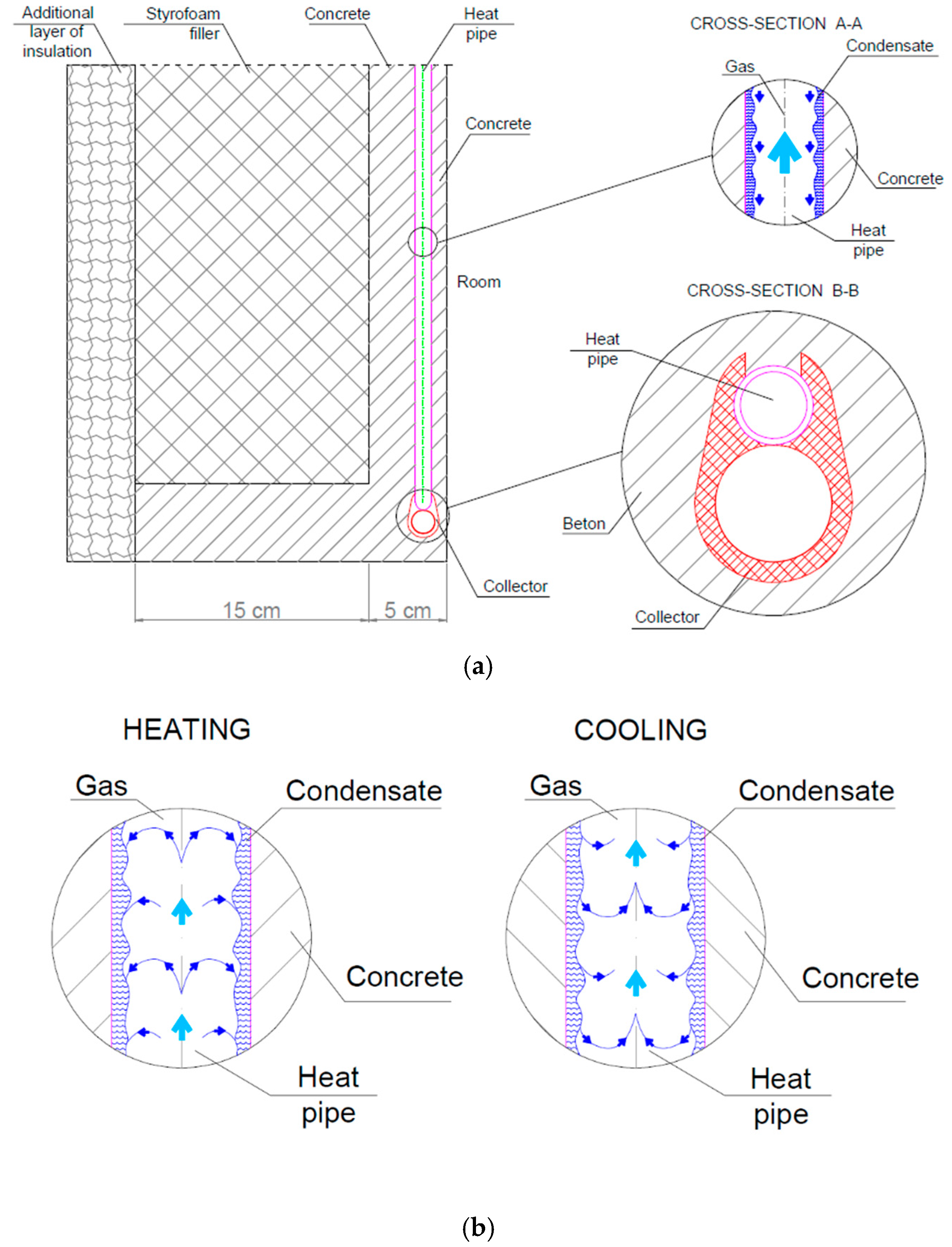
2. Description of the Tested Module

The tested heating and cooling module is a wall module with a height of h = 270 cm, a width of s = 50 cm and a thickness of δ = 20 cm. On the front side, the module contains a 5 cm thick reinforced concrete slab, in which two feed water collectors (hot and cold) are embedded, as well as a steel heat pipe filled with a phase-change thermodynamic medium. The remaining 15 cm of the module thickness is made of polystyrene. Figure 1 shows a diagram of the tested module, indicating the dimensions of the module and the location of the heating water collector and the heat pipe. One heat pipe is embedded in the module, shaped approximately in the form of a sinusoid running between the upper collectors (supplied with cold water) and the lower collectors (supplied with hot water). The horizontal parts of the tube ensure heat exchange between the supply water in the collectors and the thermodynamic medium in the heat pipes (4 × 10 cm take heat from the lower collector, and 4 × 10 cm give off heat to the upper collector). The special design of the collector, covering the heat pipe over a length of approx. 10 cm, ensures heat exchange between the thermodynamic medium in the tube and the water in the collector. However, the “contact” connection results in additional conduction resistance and reduced heat transfer efficiency (cross-section B-B in Figure 1a), compared to the location of the heat pipe part directly in the supply water stream. The vertical parts of the heat pipe (4 × 260 cm) ensure heat exchange between the thermodynamic medium and the building material of the module. Due to the significant difference in the length of the vertical and horizontal sections of the tube, it was assumed that the horizontal sections do not affect the heat exchange in the vertical sections (and vice versa). Further analyses of heat exchange between the module and the room were carried out assuming that the module contained four vertically positioned heat pipes placed 10 cm apart, and the extreme pipes were placed 10 cm from the edge of the module. The heat pipes were made of stainless steel, with a smooth surface on the inside and outside (section A-A in Figure 1a). The composition of the thermodynamic medium in the heat pipe is covered by a patent.

Placing two collectors in one module allows it to operate both in heating mode (after supplying the lower collector of the module with hot water) and in cooling mode (after supplying the upper collector of the module with cold water). In the case of heating, the thermodynamic medium in liquid form, located in the parts of the tube directly next to the hot water collector, heats up and evaporates. The steam, rising upwards, condenses on the walls of the tube, giving off heat to the tube wall and then to the concrete. The condensed liquid flows downwards, by gravity, towards the heating collector. In the case of cooling (low temperature of the cooling water), the thermodynamic medium near the collector is in the liquid state. Flowing down the tube, it heats up and gradually evaporates, taking the heat of evaporation from the tube wall (which heats the concrete). The steam, rising upwards, condenses on the cold walls of the tube in the part in contact with the cooling water collector. The condensed liquid flows downwards by gravity, evaporating along the way. The movement of the thermodynamic medium in the heat pipe in heating and cooling mode is shown schematically in Figure 1b. As can be seen from the measurements, different heat exchange processes forcing the movement of the thermodynamic medium in the pipe during heating and cooling have an effect on the different thermal parameters of the module in heating and cooling mode.

The heat transfer process between the supply water and the room can be divided into four parts. These are as follows:

• Heat transfer between the supply water in the collector and the thermodynamic medium in the heat pipe (horizontal section—cross-section B-B in Figure 1a).
• Heat transfer between the thermodynamic medium in the heat pipe and the outer surface of the heat pipe (cross-section A-A in Figure 1a).
• Heat conduction in the module material from the outer surface of the heat pipe wall to the inner surface of the module.
• Heat transfer from the surface of the module to the room (by convention and radiation).

Each of the above parts has its own specific features. The first two stages take place in thin-walled metal tubes, the heat capacity of which is negligible compared to the capacity of the rest of the module. Changes in temperature and the flow of the feed water cause almost immediate changes in the temperature of the thermodynamic medium and the temperature of the outer surface of the heat pipe. Heat exchange at these stages can be treated as a steady state. The thermal resistance in these sections is also significantly lower compared to the module material. However, heat transfer in the construction material of the module, due to the significantly higher thermal capacity of the concrete slab, must be analyzed in an unsteady state, preferably in a three-dimensional space. In addition, the building material (concrete) also has a high heat conduction resistance (compared to a heat pipe) and a non-negligible thermal capacity. This means that the building material from which the module is made has a large impact on the values of the gain factor and the values of the time constants of the module. In the process of heat transfer from the supply water to the room, a fourth stage was deliberately distinguished—heat exchange of the module surface with the room. This was due to the need to use the module surface temperature in the thermal comfort control system in the room. In a control system with the possibility of measuring the surface temperature, a significantly better quality of regulation can be achieved, which also means smaller fluctuations in the internal temperature, higher energy efficiency of the module, lower energy consumption and lower CO₂ emissions to the atmosphere. The heat exchange process in the module is reversible. Heat can be transferred from the hot supply water to the room (heating mode) or removed from the room and transferred to the cold supply water (cooling mode).

The tested heating and cooling building module is an ecological and economical solution. It was designed and manufactured to perform three utility functions:

-

As an element filling the load-bearing structure of the building (as an external partition);

-

As a heating and cooling element, supplying the room with heat or coolness as required to maintain thermal comfort; large heat exchange surfaces allow the use of low-temperature heat sources;

-

As an insulating element, limiting heat loss from the room to the external environment; on the external side, the module has additional insulation—a 15 cm thick layer of polystyrene.

The possibility of performing different functions simultaneously and their modularity mean that these modules can be manufactured outside of the construction site as prefabricated elements for direct assembly on the site. This reduces the costs and shortens the construction time of the building, and also improves the esthetics of the workmanship and energy efficiency of the product. This is an important advantage of such a solution.

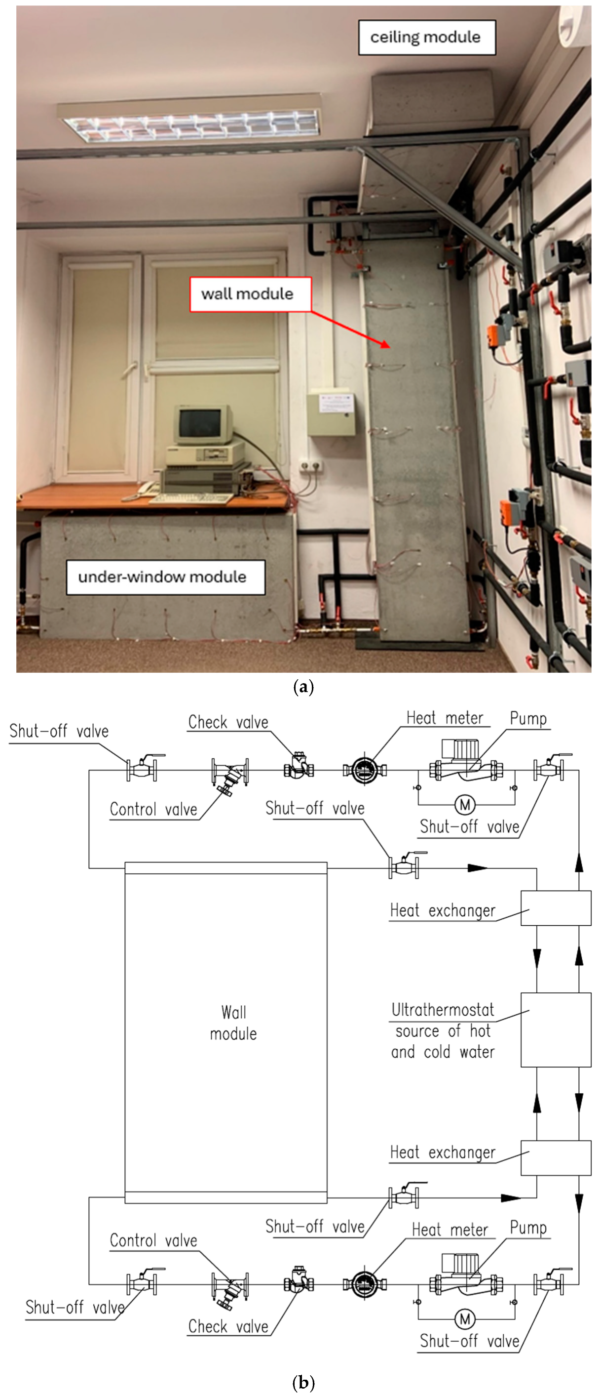
3. Research Site

3.1. Test Site View

Figure 2 shows a view of the test stand used. Three modules are installed on the stand: a wall heating and cooling module, an under-window heating module and a ceiling cooling module. This article presents the test results and analysis for the heating and cooling wall modules.

3.2. Principles (Description) of Conducting Measurements

The following parameters were measured and recorded at the station:

• Module surface temperature—11 contact sensors.
• Supply and return water temperature—4 immersion sensors.
• Internal air temperature—2 freely suspended sensors.
• Room wall temperature—1 contact sensor.
• Module supply water flow—2 water meters.

The surface temperature of the module and the internal temperature were measured using AMP-TA PT1000A contact sensors (sensor with a time constant of less than 1 s, with electric wires) AMP - Tomasz Alf Krakowska Street 304A, 32-080 Zabierzów, Poland. The temperature of the supply and return water from the modules was measured using PT1000A screw-in immersion sensors with a probe diameter of 4 mm. The declared accuracy of the PT1000A temperature sensors, in accordance with the PN-EN60751:2009 standard [37], was ±(0.15 + 0.002 ǀtǀ). The water flow measurements were carried out using ultrasonic water meters, working with Kamstrup MULTICAL 403T heat meters with PT500 sensors, with a declared accuracy of flow sensor Ef = ±(2 + 0.02 q_p/q), but not over ±5%, and a nominal flow of 0.6 m³/h (minimum reading 3 L/h) Kamstrup Sp. z o. o. street Kurzawska 9, 02-296 Warszawa, Poland.

The heat pipes were arranged in the module at a distance of 10 cm from each other and 10 cm from the side edge. It was therefore deemed advisable to place some sensors at points above the pipes and some sensors in the middle between the pipes. In order to confirm the position of the pipes in accordance with the diagrams, first of all, thermal imaging measurements of the surface temperature distribution of the radiators were performed. Their sample results, taken during heating, are shown in Figure 3a. The dark orange color and light green show the locations of the heating pipes.

However, preliminary measurements showed large differences in the surface temperature of the module, not only along its width, but also along its height. For this reason, three vertical rows of sensors were placed on the surface of the module, with three sensors in a row. The distance between the sensors horizontally was 15 cm, with the outer rows being 10 cm from the edge of the module. This arrangement of sensors meant that the middle row was placed in the middle of the heating pipes, and the outer rows were placed above the heating pipes. The distance between the sensors vertically was 87 cm, the middle horizontal row was placed in the middle of the module, and the outer rows, lower and upper, were located 48 cm from the edges and 43 cm from the heating or cooling water collectors. In addition, in the middle of the module height, on both sides, two additional sensors were placed at a distance of 5 cm from the side edges, in order to check the effect of the side surfaces of the module on the value of the front surface temperature. In total, this consisted of 11 surface sensors and 4 immersion sensors for measuring the temperature of the water flowing into and out of the module, and 2 internal air temperature sensors (in the upper and lower part of the module, at a distance of 25 cm from the edge of the module). The approximate arrangement of the measuring sensors on the modules is shown in Figure 3b.

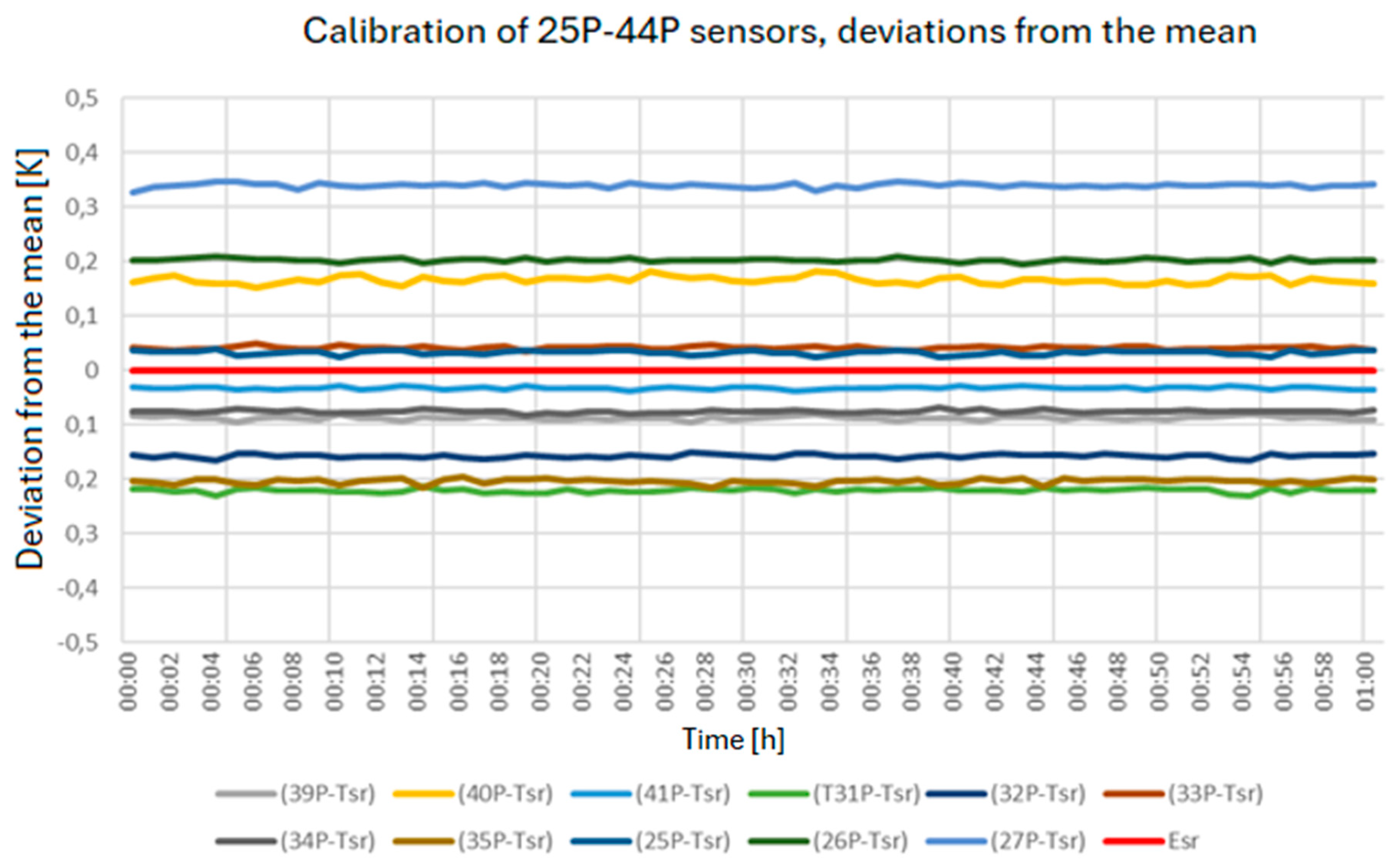
3.3. Calibration of Measuring Sensors

Before taking the measurements, the temperature measuring sensors used for testing the temperature distribution on the module surface were calibrated. Due to the type of sensors and their large number (11 sensors for a single module), it was not possible to perform the classic calibration method, i.e., by immersing them in ice water at a temperature of 0 °C. In contact sensors, the connection of electrical signal wires to the sensor is not waterproof. Therefore, immersing them in ice water was excluded. Also, placing all sensors in a waterproof container filled with air and immersing this in water caused a temperature gradient and significant differences in the sensor readings. For this reason, a non-standard calibration procedure was decided upon. In the first step, the module surface temperature was measured in a steady state at a supply water temperature equal to the internal air temperature. After this, all the sensors should indicate the same temperature value. Then, the calculated average value of the readings of all sensors and the errors of the readings were calculated as the difference between the reading of a given sensor and the average value of the readings of all sensors. The calibration results are presented in Figure 4 and

Table 1. The differences in the indications (errors) of the sensors mounted at the module surface.

Sensor Marking	25P	26P	27P	31P	32P	33P	34P	35P	39P	40P	41P	42P	43P	44P
Indication errors [K]	0.01	0.19	0.34	−0.24	−0.18	0.01	−0.11	−0.24	−0.11	0.12	−0.08	−0.05	0.14	0.20

.

4. Measurements and Results Processing

During the tests, series of measurements of step characteristics were performed in two modes of module operation, i.e., heating and cooling, at different flow values and supply water temperatures. In the cooling mode, three measurement series were performed for flows V = 100 L/h, 50 L/h and 15 L/h. At a flow of V = 100 L/h, the water temperature was reduced in a stepwise manner, every 5 K, from ~25 °C to ~10 °C (from 26↘20↘15↘10 and then from 10↗15↗20↗26). At flows V = 50 L/h and 15 L/h, the water temperature was reduced, also in a stepwise manner, but every 10 K, from ~25 to ~6 °C (26↘16↘6↗16↗26). The reason for increasing the amplitude of the supply water temperature change from 5 to 10 K was that the changes in the temperature value on the module surface were too small when the supply water temperature changed by 5 K. In the heating mode, three measurement series were also performed for flows V = 120 L/h, 60 L/h and 30 L/h, with a step change in the supply water temperature: the water temperature was changed every 15 K, from ~20 to ~35, and then from ~35 to ~50 °C. The Simex measuring system, with 16 bit analog-to-digital temperature converters, was used to record the measurements. The measurements were taken with a step of 1 min, and the data were recorded at each reading step.

The supply water temperature range for the cooling mode was adjusted to typical temperatures occurring in the range of chilled water installations used in cooling installations, taking into account the risk of condensation on the module surface. The tested flow range of the water supplying the heating and cooling collectors was adjusted to the capacity of the measurement station and the applied water flow rates in the heated and chilled water installations. The above parameters were selected in such a way as to examine the operation of the modules in connection with typical parameters of internal heating and cooling installations; thanks to this, the obtained results will allow the determination of the usability of the modules in correlation with their cooperation with real, typical building installations. In cooling mode, the most commonly used cold water temperature in air conditioning is 6 °C. When changing the cooling capacity of the module, it can change from 6 °C to the internal temperature, i.e., 26 °C. In heating mode, the module can operate with water supply from an internal temperature of 20 °C to approx. 50 °C (low-parameter—heat carrier obtained from renewable energy or waste heat), or with water supply at a temperature of up to approx. 90 °C (high-parameter heat carrier).

For each step characteristic, the following were developed:

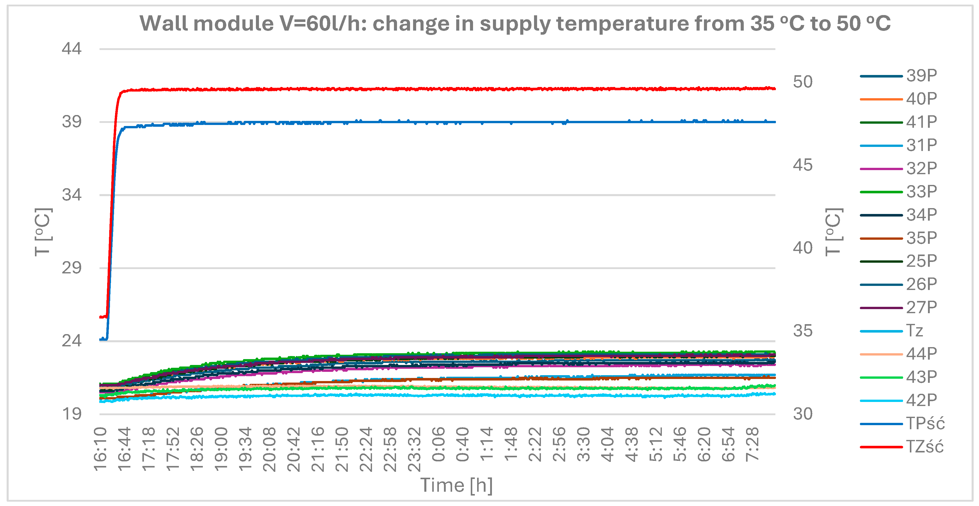
• A graph of the temperature values on the module surface (from all sensors);
• A graph of the internal temperature values and the temperature of the building partition;
• A graph of the temperature values from each row (vertical and horizontal) of sensors;
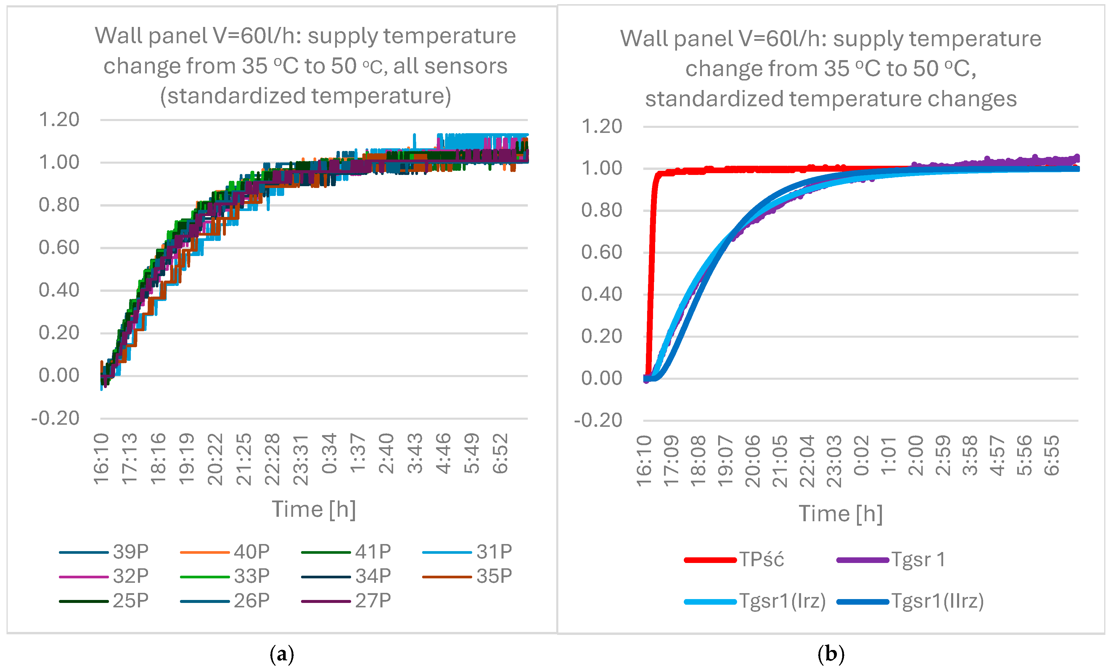
• A graph of the standardized temperature values on the module surface;
• Calculations (identification) of the values of the amplification coefficients and time constants of the inertial models adopted to describe the transient states (dynamics) of the module;
• Calculations of the heat flux transferred to the room or assimilated from the room in steady states.

Figure 5 presents a summary graph of the thermal power of the tested module in the steady state: in cooling mode (Figure 5a) and in heating mode (Figure 5b). The initial temperature difference was defined as the temperature difference of the heat exchange medium, i.e., the difference between the values of the supply water temperature and the internal air temperature.

From the position of the points in Figure 5, it can be concluded that in the cooling mode, the change in the thermal power of the module as a function of the initial temperature difference is much smaller than the change in power in the heating mode. In the tested range of the change in the initial temperature difference from 3 to 15 K, the power of the module in the cooling mode increases by ~30% (relative to the maximum power). A slight increase in power can also be seen when increasing the cooling water flow. In the heating mode, the power of the module increases significantly with the increase in the initial temperature difference. This increase is the fastest at the greatest heating water flows. The difference in the thermal power of the module in the cooling and heating mode results from the principle of operation of the heat pipe, and specifically from the movement of the thermodynamic medium vapor inside the pipe in the heating and cooling mode.

In the cooling mode, the driving potential of the thermodynamic medium’s movement is the higher temperature of the module material (concrete). The temperature value of the module’s building material changes within a small range (within ~5 K), so the change in power is not large.

In the heating mode, the driving potential of the thermodynamic medium’s movement is the higher temperature of the supply water. The value of the supply water temperature varies within a wide range (within ~30 K), and therefore the change in power is greater. In the tested range, from 10 to 50 K, the power changes by ~75% in relation to the maximum value.

The next stage of the results development was the identification of parameters characterizing the static and dynamic properties of the building module as a control object. When identifying control objects, thermal processes are most often described by inertial models [34,35,36]. The accuracy of the description of the static and dynamic properties of the tested module was analyzed using two linear inertial models in the following forms:

$$\text{- }\mathrm{a}\mathrm{first}\text{-}\mathrm{order}\mathrm{inertial}\mathrm{model}\mathrm{with}\mathrm{a}\mathrm{delay}{G}_I\left(s\right)={\displaystyle \frac{k}{Ts+1}}{e}^{{-T}_{0}s}$$

(1)

and

$$\text{- }\mathrm{a}\mathrm{second}\text{-}\mathrm{order}\mathrm{inertial}\mathrm{model}\mathrm{with}\mathrm{a}\mathrm{delay}{G}_I\left(s\right)={\displaystyle \frac{k}{{(T}_{1}s+1){(T}_{2}s+1)}}{e}^{{-T}_{0}s}$$

(2)

where

• k—amplification factor, dimensionless;
• T, T₁, T₂—time constants, min;
• T₀—delay time, min.

The amplification factor is defined as the quotient of the change in the temperature value on the module surface (t_M) and the change in the initial difference between the temperature of the water supplying the module (t_s) and the temperature of the internal air (t_i), i.e., as follows:

$$k={\displaystyle \frac{{∆t}_M}{∆\left(t_s-t_i\right)}}$$

(3)

The values of the amplification coefficient k and the delay time T₀ are the same for both models. The delay time T₀ is defined as the transport delay time, i.e., as the time from the moment of introducing a change in the supply water temperature to the moment of a noticeable change in the average value of the module surface temperature caused by this change.

Due to the considerable height of the module, the uniformity of the temperature distribution along its height was also examined, i.e., at a distance of 43 cm, 130 cm and 217 cm from the supply water collector. This action resulted from the need to find a place on the module surface where the measured temperature value would be the closest to the average temperature value from the entire module surface. This would be the so-called representative temperature measurement location recommended for the location of the module’s power control system sensor. The control system usually uses one sensor, so its correct location is crucial in this case.

Figure 6 shows sample graphs of measurement data from the heating period at a flow rate of V = 60 L/h, with the feed water temperature increasing from 35 °C to approx. 50 °C.

Based on the measurement results (including the graph in Figure 6), four characteristic features of the temperature change on the module surface can be observed:

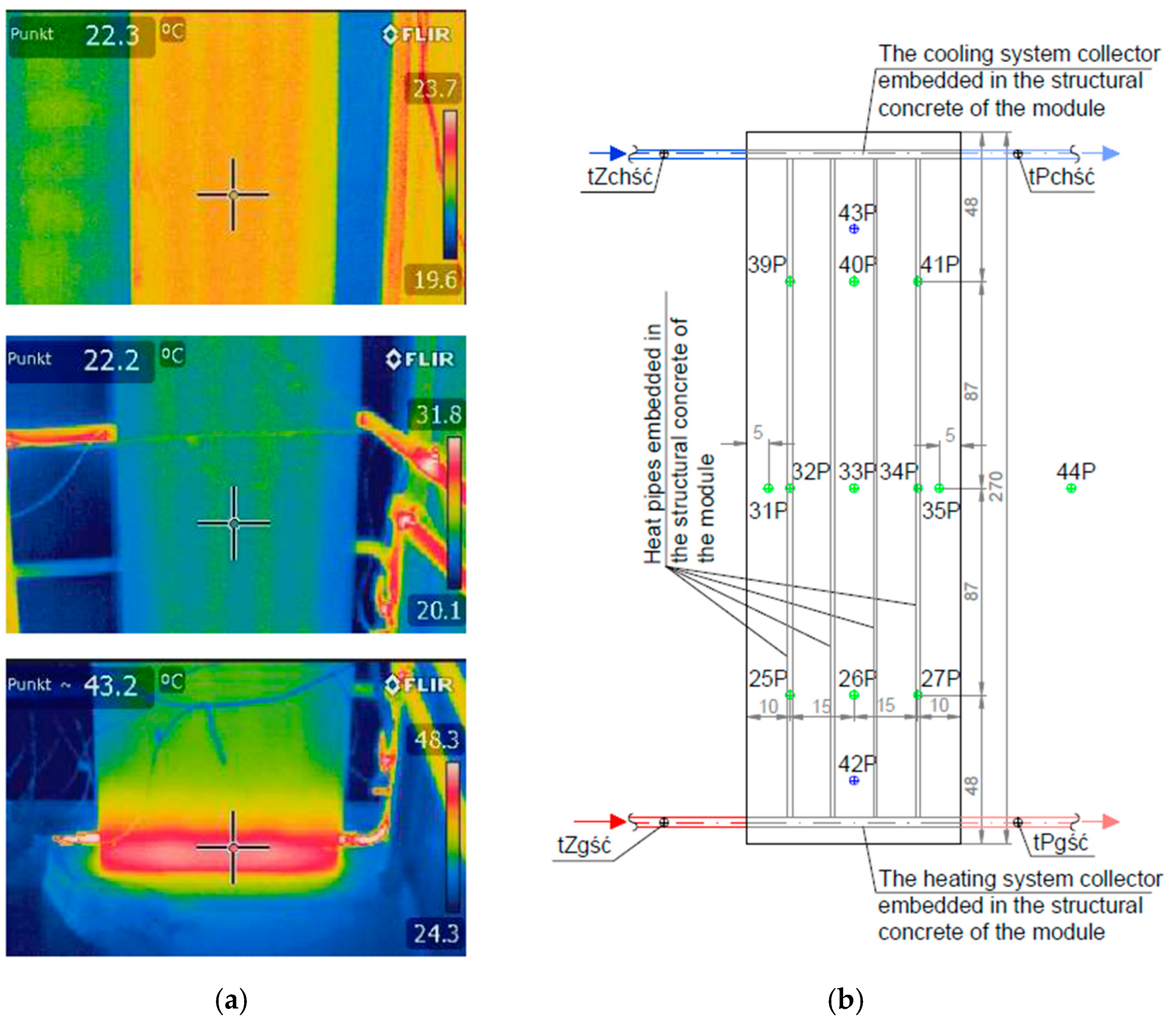
• Relatively small changes in the module surface temperature. As shown in the figure, a change in the module supply water temperature of approx. 15 K causes a temperature change on the module surface of 1.5–2.0 K. This indicates low heat exchange efficiency and low values of the k amplification factor in the adopted inertial models. Low heat exchange efficiency is also the reason for introducing forcing (changes in supply water temperature) of relatively large values, in order to obtain significant changes in the module surface temperature.
• Relatively large variation in the temperature distribution on the module surface. Temperature values at different points on the module surface differ from each other by approx. 1.2 K. Changes in values are particularly visible with the change in module height.
• Relatively slow changes in the module surface temperature. After changing the supply water temperature, it takes 8–10 h to establish a new temperature value on the module surface.
• The nature of the change in the module surface temperature at different measurement points is similar; clear differences occur in the steady-state temperature values.

The above features have a significant impact on the operation of the control system and the accuracy of maintaining the internal temperature in the room. They influence the selection of the structure and parameters of the control algorithm and the choice of the mounting location for the measuring sensor.

As it results from the above-mentioned feature no. 4, the nature of the change in the module surface temperature at different measurement points is similar; clear differences occur in the temperature values in the steady state. Large differences would require the calculation of model parameters for each measurement point, which would significantly increase the time required for processing the results. For this reason, it was decided to standardize the temperature changes. The standardized temperature value was calculated in relation to the temperature difference between the final and initial values in steady states, i.e., in accordance with the following formula:

$$t^{\ast }(\tau )={\displaystyle \frac{t\left(\tau \right)-t_{u1}}{t_{u2}-t_{u1}}}$$

(4)

where

• t(τ)—temperature value at the analyzed time instant, °C;
• t_u1—temperature value in the steady state, before the change in the supply water temperature, °C;
• t_u2—temperature value in the final steady state, °C.

The value of the standardized temperature is dimensionless, and always varies in the range of 0 to 1.

The course of change in the standardized temperature values at individual measurement points is shown in Figure 7. A clear improvement in the agreement of the curves can be seen. The only measurement points with a different course are the extreme points in the middle row, located 5 cm from the edge (sensors marked in Figure 4 as 31P and 35P). When calculating the time constants of the inertial models, these points were omitted. The values of the time constants of the inertial models were determined based on standardized step characteristics using the method of moments:

-

Zero-order for the first-order inertial model (when calculating the time constant T),

-

Zero- and first-order for the second-order model (when calculating the time constants T₁ and T₂).

The zero-order moment (M₀) and the first-order moment (M₁) for a standardized characteristic with a range of value change from 0 to 1, recorded with a unit step (1 min), can be calculated using the following formulas (Douglas [34]):

$$M_0={\int }_0^{\mathrm{\infty }}\left[{1-t}^{\ast }\left(\tau \right)\right]d\tau ={\sum }_{k=0}^{k=n}\left[1-t^{\ast }\left(k∆\tau \right)\right]$$

(5)

$$M_1={\displaystyle \frac{1}{M_0}}{\int }_0^{\mathrm{\infty }}\tau \ast \left[{1-t}^{\ast }\left(\tau \right)\right]d\tau ={\displaystyle \frac{1}{M_0}}{\sum }_{k=0}^{k=n}\left(k∆\tau \right)\ast \left[1-t^{\ast }\left(k∆\tau \right)\right]$$

(6)

$$T=M_0,T_1={0.5M}_0+\sqrt{(4M_1-3)},T_2={0.5M}_0-\sqrt{(4M_1-3)}$$

(7)

where

• k—next time step in measuring the step characteristic;
• n—number of time steps from the initial steady state to the final steady state of the step characteristic;
• ∆τ—data recording step (1 min).

An example of the course of standardized temperature changes obtained from measurements and inertial models for the calculated time constants T, T₁ and T₂ is shown in Figure 7. The curves measured and obtained from the first-order inertial model practically coincide.

5. Analysis of Measurement Results

5.1. Module Operation in Cooling Mode

Table 2. The values of the gain coefficient k for the tested module, calculated based on Formula (3), in the cooling mode.

No	Cooling Water Flow [L/h]	Reducing the Cooling Water Temperature [Tzas↘]			Increasing the Cooling Water Temperature [Tzas↗]
		(*) 43	(*) 130	(*) 217	(*) 43	(*) 130	(*) 217
1	100	0.382	0.333	0.271	0.182	0.146	0.087
2	50	0.287	0.244	0.193	0.164	0.117	0.065
3	15	0.264	0.204	0.149	0.155	0.123	0.070

(*)—distance of the measuring point from the cooling water collector in cm. ↘ temperature drop. ↗ temperature rise.

and the graphs in Figure 8 show the values of the amplification coefficient calculated according to relationship (3), obtained from measurements taken when the module was operating in cooling mode. The table shows the average values from measurements of the same type, i.e., for each flow, the average values of the k coefficient obtained from all measurements when the temperature of the water supplying the collector was reduced (columns 3–5 in Table 2), and the average values of the k coefficient obtained when the temperature was increased (columns 6–8 in Table 2).

The curves on the graphs show a large influence of the direction of the change in the cooling water temperature and the distance of the measuring point from the collector, and a smaller influence of the water flow. The value of the k coefficient decreases with the increase in the distance of the measuring point from the collector (Figure 8a). This relationship is approximately linear. Between the measuring points closest to (43 cm) and furthest from (217 cm) the collector, the amplification factor k decreases from 1.4 to 2.5 times, depending on the value of the flow and the direction of the change in the cooling water temperature. The dependence of the k coefficient on the flow is only significant when the supply water temperature is reduced. It can be approximated by a straight line for turbulent flow. For a small laminar flow with an increase in the supply water temperature, the k values are practically constant.

The probable cause of higher values of the amplification factor is the change in the nature of heat exchange in the heat pipe. At low values of the supply water temperature and higher values of the module material temperature, the thermodynamic factor evaporates from the pipe wall. At higher values of the supply water temperature and lower values of the module material temperature, the thermodynamic factor condenses on the pipe wall. Simulations of the heat exchange process between supply water-building module-room in the numerical model being constructed should explain this fact.

Table 3. List of averaged values of inertial model parameters in cooling mode.

No	Description	First-Order Model		Second-Order Model
		T	(*) std	T1	T2	(*) std
		min	-	min	min	-
Cooling—all sensors
1	V = 100 L/h, Tzas↘	252.4	0.0477	154.2	98.2	0.0525
2	V = 50 L/h, Tzas↘	274.5	0.0403	166.7	107.9	0.0556
3	V = 15 L/h, Tzas↘	303.9	0.0351	183.3	120.7	0.0650
4	V = 100 L/h, Tzas↗	103.6	0.0758	64.7	38.8	0.0742
5	V = 50 L/h, Tzas↗	141.9	0.0540	94.6	47.3	0.0410
6	V = 15 L/h, Tzas↗	148.2	0.0449	96.0	52.2	0.0516
Cooling—mid-row sensors
7	V = 100 L/h, Tzas↘	198.3	0.0303	124.9	73.4	0.0556
8	V = 50 L/h, Tzas↘	238.9	0.0236	147.9	91.0	0.0591
9	V = 15 L/h, Tzas↘	272.2	0.0284	166.4	105.8	0.0605
10	V = 100 L/h, Tzas↗	110.3	0.0427	74.2	36.1	0.0482
11	V = 50 L/h, Tzas↗	153.1	0.0271	99.1	54.0	0.0469
12	V = 15 L/h, Tzas↗	159.6	0.0349	102.9	56.7	0.0430

(*) std—standard deviation of the standardized characteristic. Tzas—supply water temperature. ↘ temperature drop. ↗ temperature.

and Figure 9 present values of time constants and standard deviations as measures of the accuracy of representing the heat exchange process using first- and second-order inertial models.

The parameters in Table 3 and in Figure 9 were calculated for the following two cases:

-

Using measurements from all sensors,

-

Using measurements only from the sensors located in the middle of the module (l = 130 cm).

The calculation of the parameters only for the sensors located in the middle of the module was performed with the aim of checking whether the values of time constants changed with the location of the measuring point, and investigating what differences there were in the values of the time constants calculated from the averaged values of the indications of all the sensors placed on the surface of the module, compared to the values of the time constants from the indications of the sensors located in the middle of the module. Module power control systems most often use only one measuring sensor, so their location is important for their correct operation. The most commonly used location is the middle of the module. As can be seen from Table 3, the calculation results using measurements from all the sensors mounted on the module, and the measurements from the sensors located in the middle of the module, are similar. Higher values of time constants were obtained for all the sensors; in the case of an increase in the water temperature in the collector, they are on average 5% lower, and in the case of a decrease in the temperature, they are higher than 14%.

It should be emphasized, however, that the values of the time constants change in a wide range, depending on the flow rate and the direction of the change in the supply water temperature. The lowest value (103.6 min) of the time constant of the first-order model was obtained at a flow rate of 100 L/h and an increasing value of the cooling water, and the highest value (303.6 min) was obtained at a flow rate of 30 L/h and a decreasing value of the cooling water. The direction of temperature change has a greater effect on the values of the time constants, and the cooling water flow has a smaller effect. The values are also greater when the cooling water temperature is reduced than when it is increased (approx. 2 times greater values). The changes in the time constants of the second-order inertial model are analogous. Their values are greater when the cooling water temperature is reduced than when it is increased (approx. 1.5 times). The changes in the values when the water flow is changed are also much smaller.

The delay time ranged from 10 to 30 min, with the average values being as follows:

-

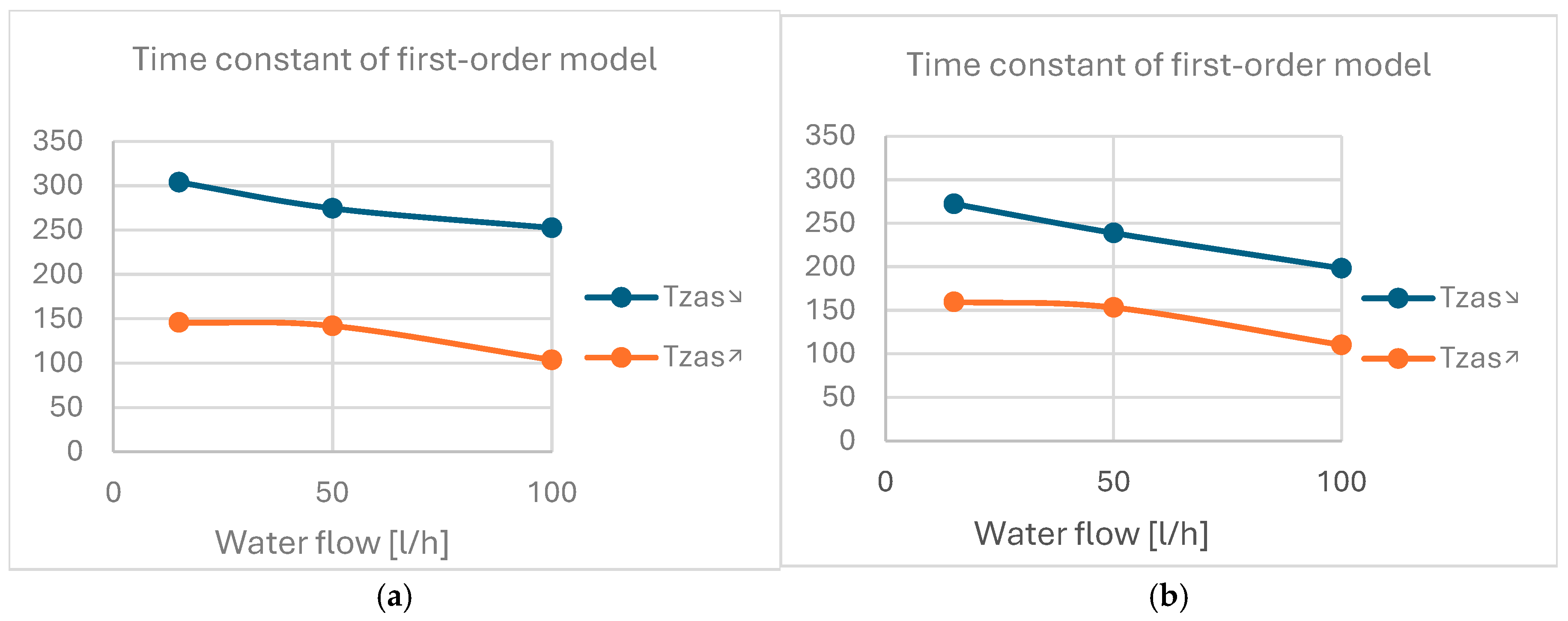
22.5 min when decreasing the temperature for all the sensors on the module surface;

-

12.5 min when increasing the temperature for all the sensors on the module surface;

-

20.5 min when decreasing the temperature for the middle-row sensors of the module;

-

16.0 min when increasing the temperature for the middle-row sensors of the module.

The inaccuracy of the description of the dynamic properties of the module using first- and second-order inertial models was assessed using the standard deviation between the curve obtained from the model and from the measurements. The standardized characteristics calculated according to relationship (4) were compared. The value of the standard deviation was calculated using the following formula:

$$std=\sqrt{{\displaystyle \frac{1}{n-1}}\sum _1^n{\left(t_p^{\ast }-t_m^{\ast }\right)}^2}$$

(8)

where

• $t_p^{\ast }$—the averaged standardized temperature value obtained from the measurements;
• $t_m^{\ast }$—the standardized temperature value obtained from the model;
• n—the number of measurement steps in the characteristics of standardized variables.

From assessing the inaccuracy of the description of the dynamic properties of the module using the first- and second-order inertial models, it can be stated that higher accuracy is obtained using the first-order inertial model. For this model, the inaccuracy for individual series is within the range of 2.4–7.6% of the temperature change range, with an average value of 4.0%. For the second-order inertial model, the range of change in the standard deviation is 4.1–7.4%, with an average value of 5.4%. This means that when the module surface temperature changes by 1 K, the inaccuracy of calculating its value at a specific time instant is, on average, 0.04 K for the first-order inertial model and 0.054 K for the second-order inertial model.

5.2. Module Operation in Heating Mode

Similarly to the cooling mode,

Table 4. The values of the gain coefficient k for the tested module, calculated based on Formula (3) in the heating mode.

No	Heating Water Flow [L/h]	Reducing the Heating Water Temperature			Increasing the Temperature of the Heating Water
		(*) 43	(*) 130	(*) 217	(*) 43	(*) 130	(*) 217
1	30	0.175	0.161	0.170	0.089	0.078	0.087
2	60	0.199	0.179	0.178	0143	0.130	0.127
3	120	0.211	0.192	0.198	0.156	0.153	0.163

(*)—distance of the measuring point from the cooling water collector, in cm.

and Figure 10 contain the values of the gain coefficient calculated according to relationship (3), obtained from the measurements taken when the module was operating in the heating mode. The table contains the average values from the same type of measurements (similarly to the cooling mode).

Similarly to the cooling mode, the curves in Figure 10 show the influence of the same factors in the heating mode, i.e., the direction of temperature change, the value of the heating water flow rate and the distance of the measuring point from the supply water collector. However, the nature of these dependencies is different. The supply water flow rate has the greatest influence, while the distance from the collector has the smallest influence. The direction of temperature change has a significant influence on the nature of the dependence of the k coefficient on the flow rate. During cooling and temperature increase, the value of the k amplification factor changes slightly with the increase in flow rate. In the case of heating, this dependency is analogous, but the dependency is definitely stronger. Increasing the flow rate increases the heat exchange intensity (larger/faster evaporation of the thermodynamic medium). In the case of decreasing temperature, the nature of the change in the k coefficient is the same for heating and cooling; however, the increase in the k coefficient value for heating is smaller than that for cooling. The slopes of the k value change curves for heating are almost twice as small as the slopes of the curves for cooling.

Table 5. List of averaged values of parameters of substitute models for heating.

No	Description	First-Order Model		Second-Order Model
		T	(*) std	T1	T2	(*) std
		min	-	min	min	-
Heating—all sensors
1	V = 120 L/h, Tzas↘	189.7	0.259	120.7	69.1	0.063
2	V = 60 L/h, Tzas↘	221.4	0.0177	138.8	82.6	0.0574
3	V = 30 L/h, Tzas↘	192.2	0.0173	122.9	70.3	0.0578
4	V = 120 L/h, Tzas↗	143.1	0.0201	95.4	47.7	0.0545
5	V = 60 L/h, Tzas↗	123.2	0.0138	82.4	40.8	0.0410
6	V = 30 L/h, Tzas↗	106	0.0299	71.8	34.2	0.0447
Heating—mid-row sensors
7	V = 120 L/h, Tzas↘	149.5	0.0169	98.2	51.3	0.0556
8	V = 60 L/h, Tzas↘	217.6	0.0218	136.9	80.7	0.0632
9	V = 30 L/h, Tzas↘	208.4	0.0225	130.9	77.5	0.0532
10	V = 120 L/h, Tzas↗	163.2	0.0466	103.8	59.4	0.0261
11	V = 60 L/h, Tzas↗	127.2	0.0157	84.7	42.6	0.0451
12	V = 30 L/h, Tzas↗	112.1	0.0387	75.3	36.8	0.0482

(*) std—standard deviation of the standardized characteristic. Tzas—supply water temperature↘ temperature drop; ↗ temperature.

and Figure 11 show the values of the time constants and their standard deviation in heating mode.

As can be seen from Table 5, the calculation results using the measurements from all the sensors mounted on the module, and the measurements from the sensors located in the middle of the module, are similar. The differences between the values of the time constants during heating are even smaller than during cooling. The changes in the values of the time constants when changing the flow and the direction of change in the supply water temperature also decrease. The smallest value (106.3 min) of the time constant of the first-order model is obtained at a flow of 30 L/h and an increasing temperature value, and the largest (208.4 min) is also obtained at a flow of 30 L/h and a decreasing temperature value. The direction of temperature change has a greater effect on the values of time constants than the heating water flow. The changes in the time constants of the second-order inertial model are analogous.

The delay time ranged from 10.7 to 22.7 min, with the average values being as follows:

-

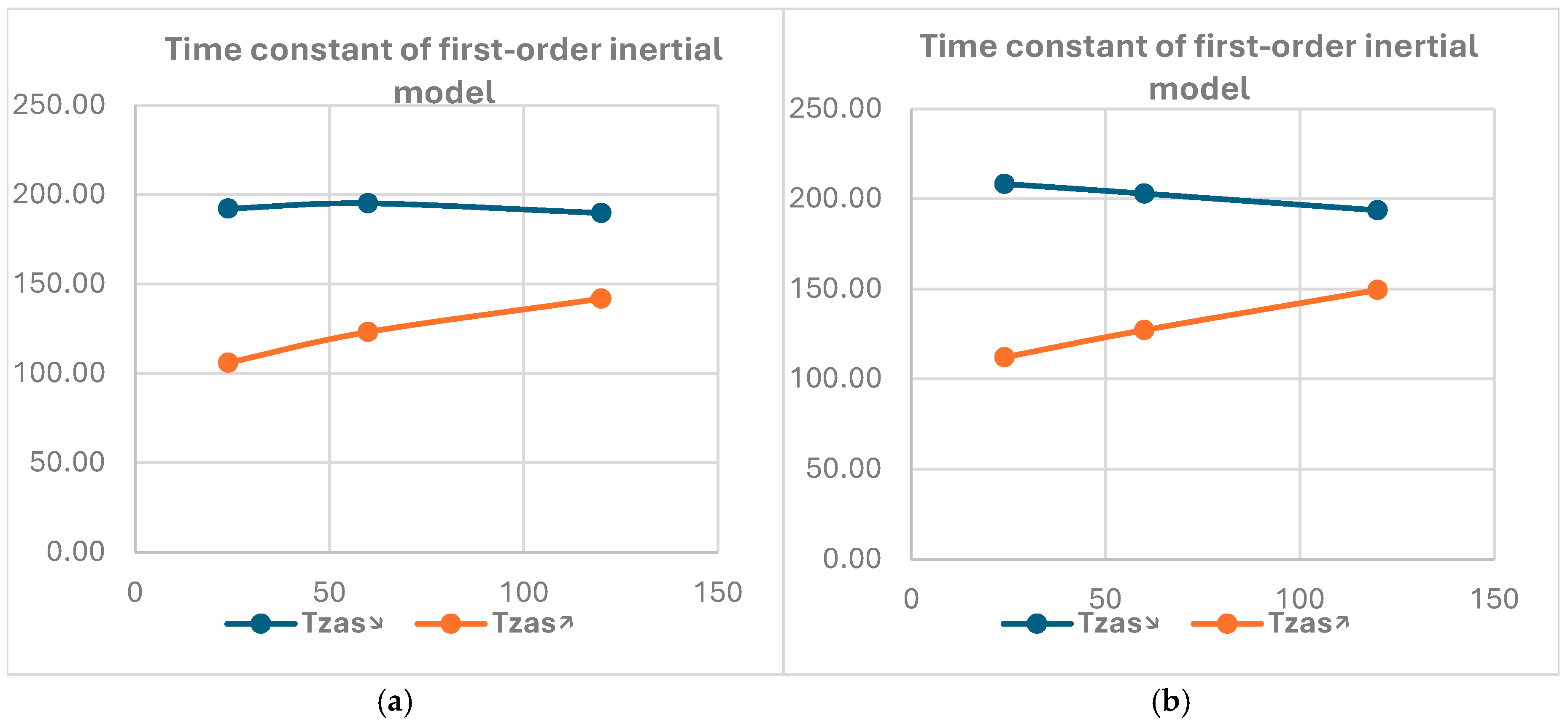
22.7 min when decreasing the temperature for all the sensors on the module surface;

-

10.7 min when increasing the temperature for all the sensors on the module surface;

-

17.0 min when decreasing the temperature for the middle-row sensors of the module;

-

15.8 min when increasing the temperature for the middle-row sensors of the module.

Table 6. A summary of the influence of selected factors on the changes in the gain coefficient k and the time constant T.

Cooling Period
Effect	Cause	The power of influence
Higher values of k are obtained	-at a smaller distance of the point from the collector	high
	-when the cold water temperature drops than when it increases	high
	-for larger flows of cold water	small
The k values do not change	-with increasing cold water flow	no influence
Smaller T values are obtained	-when the cold water temperature increases than when it decreases	high
	-for larger flows of cold water	small
Heating period
Effect	Cause	The power of influence
Higher values of k are obtained	-when the hot water temperature drops than when it increases	high
	-for larger flows of hot water	small
The k values do not change	-when changing the distance from the collector	no influence
Smaller T values are obtained	-when the hot water temperature increases than when it decreases	high
	-for larger flows of hot water	small
	-with lower flows and increased hot water temperature	small

lists the most important factors influencing the values of the amplification coefficient k and the time constants T, indicating the strength of their influence.

6. Summary and Conclusions

The tests conducted on the heating and cooling wall modules allow for analysis and generalizations regarding the formation of parameters characterizing their thermal properties. Two characteristic areas of analysis can be distinguished here.

6.1. Influence of Design Parameters on Power of Heat Pipe Module

Thermal power depends on many factors. Based on the test results, it can be concluded that the following factors have the greatest influence on the power of the module:

• The type of thermodynamic medium used in the tubes;
• The thermal resistance and heat exchange surface between the heat pipe and the feedwater collector;
• The spacing (distance from each other) of the heat pipes in the module;
• The arrangement of reinforcing ribs in the concrete of the module (in the case of reinforced concrete modules).

The above factors are defined at the stage of module construction, and do not change during operation. However, the correctness of the adopted solutions can be assessed based on the measurement results.

Ad. 1. The adopted thermodynamic medium is covered by a patent. It is only known that it is an aqueous solution of alcohol of unknown proportion. The basic parameters of the thermodynamic medium components [8] seem to be correct:

• Methanol—operating range 10–130 °C, melting point −98 °C, boiling point 64 at atm. press. °C;
• Ethanol—operating range 10–130 °C, melting point −112 °C, boiling point 78 at atm. press. °C;
• Water—operating range 30–200 °C, melting point 0 °C, boiling point 100 at atm. press. °C.

The problem comes down to the proportions of the components.

The pressure in the heat pipe is also unknown. A low thermal power of the module and low values of the amplification factors indicate insufficient evaporation of the thermodynamical medium, which suggests that the concentration of alcohol in the mixture is too low. An alternative solution is to create a vacuum in the tube, which would also increase the intensity of evaporation of the thermodynamic fluid. When selecting a thermodynamic medium, the aspect of module failure in the form of a heat pipe leak and the penetration of the thermodynamic fluid into the building module is important. In order to minimize the effects of such a failure, the thermodynamic medium should be colorless and odorless (neutral in smell). It also cannot cause leaks into the building material or release chemicals harmful to the health of the users of the premises. It would be best if after the tube leak, the released medium is in the form of a gas (at ambient temperature and at atmospheric pressure). The tested model meets these requirements.

Ad. 2. The thermal resistance and the heat exchange surface between the heat pipe and the feed water collector result from the applied connection of the pipe with the collector. In the tested module, the heat exchange surface between the thermodynamic medium and the water in the collector is almost 10 times smaller than the heat exchange surface between the thermodynamic medium and the building material of the module (the external surface of the heat pipe adjacent to the building material). In addition, the pipe–collector connection is a “butt”-type connection, which also means additional conduction resistance of the collector material. The effect is a much higher heat flux density at this connection compared to the heat flux density at the heat pipe–building material connection. According to the authors, this is the main reason for the low thermal power of the module in both the heating and cooling modes.

Ad. 3. The distance between the heat pipes in the building material is another important factor influencing the power of the module. Considering the construction of the tested module, it can be assumed that its power is approximately proportional to the number of pipes. It can therefore be expected that placing more pipes vertically, at a smaller distance from each other, would increase the power of the module. For example, placing nine pipes at a distance of 5 cm from each other (instead of the current 10 cm) would increase the power of the module more than two times.

Ad. 4. The method of arrangement and connection of the reinforcing steel elements in the module material is another factor influencing the uniformity of the temperature distribution on the module surface. The thermal conductivity coefficient of steel is definitely (~100 times) higher than that of concrete, which increases the heat flux density in the building material of the module and accelerates its distribution. An additional effect is the reduction in the time constants of the module, which would improve its regulatory properties. It seems that the best solution would be a reinforcing steel mesh with low thermal resistance (especially at the connections between the mesh holes), integrated with the outer diameter of the tube. The cross-section of the reinforcing mesh should be selected so as to ensure the required strength parameters of the module.

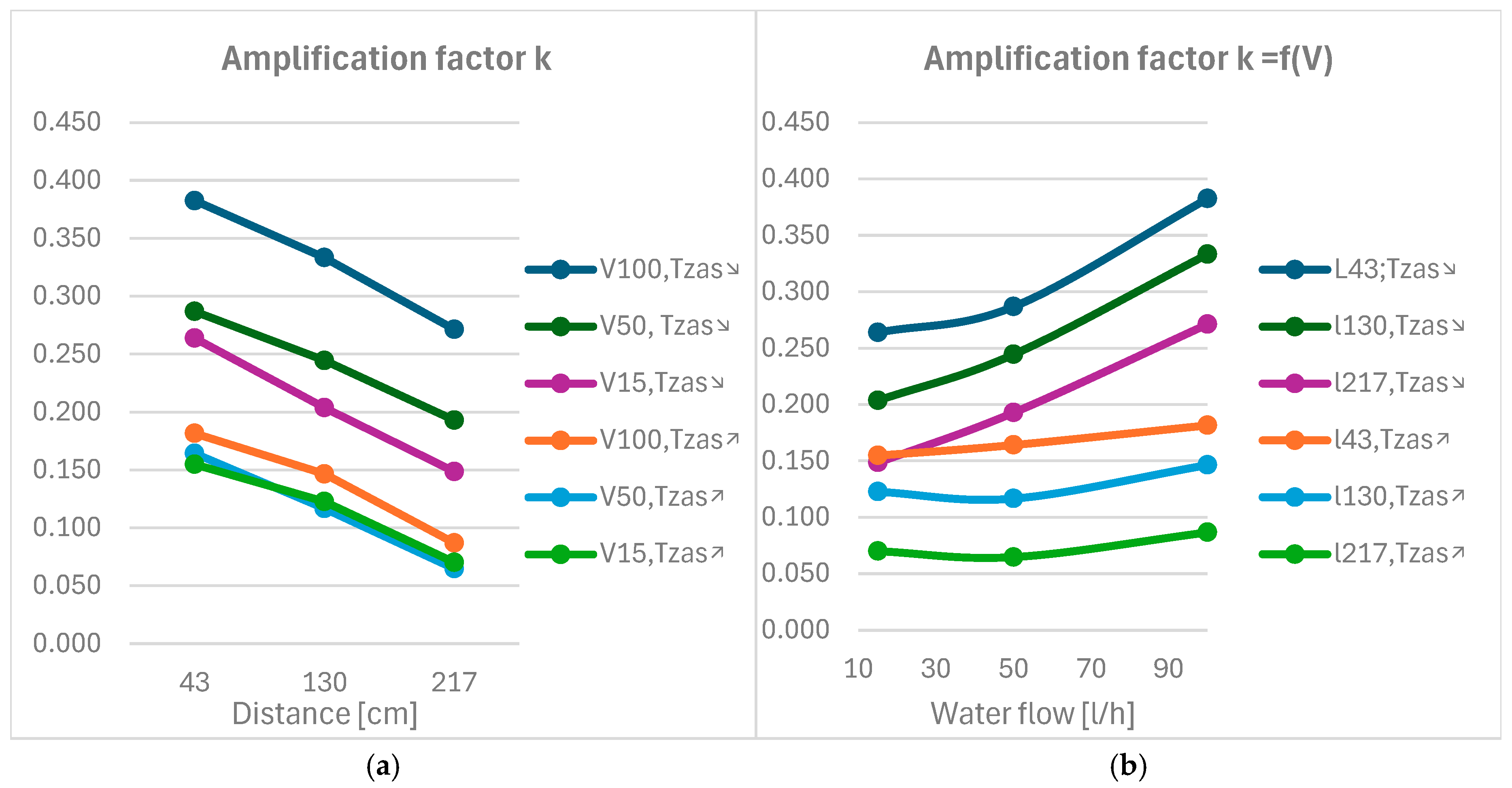
6.2. Influence of Operating Conditions on Control Parameters

The design factors of the building module also have a significant influence on its behavior during operation. The influence of the thermal control parameters of the module on its operation is analyzed below. The following findings were obtained:

• small values of the gain coefficient allow the use of larger values of the initial temperature difference in operation;
• significantly larger changes in the values of the power and gain coefficients cause larger temperature changes than changes in the feed water flow;
• large changes in control parameters require complex, individual control algorithms; with variable room heat demand, the algorithm should have a procedure for forecasting the required module power in a time horizon of 1–2 h.

Ad 1. Small values of the amplification coefficient allow the use of larger values of the initial temperature difference, i.e., the difference between the supply water temperature and the internal air temperature. The limitation lies in the temperature values that cause the following:

-

Moisture condensation on the cold surface of the module in cooling mode;

-

Deterioration of the thermal comfort of users in heating mode, due to the high radiation temperature of the walls.

Moisture condensation in cooling mode depends on the building climate zone, internal moisture gains and room ventilation. During the tests, lowering the supply water temperature to 10 °C caused a decrease in the average module surface temperature from ~26 to ~21 °C, without moisture condensation on the module. In turn, during heating, the module surface temperature should not be higher than the internal air temperature by more than 10 °C [38].

Ad. 2 The fact that changes in temperature values have a much greater impact on the change in power and coefficient gain values then changes in flow rate values, prefer “qualitative regulation” in the room temperature control system. This requires a control using a 3-way valve and an additional pump for each room, which will undoubtedly increase the cost of the control system. It should be noted that this feature is not an individual feature of the tested module. The fact that the module power is more strongly dependent on temperature than on the supply water flow is confirmed by studies conducted on other module designs with heat pipes, e.g., [29].

Ad. 3 Large changes in the module control parameters, including large values of time constants and a strong dependence of the gain coefficient on the direction of the change in the supply water temperature, require complex control algorithms. Standard control algorithms, or a cascade structure of the control system, may prove insufficient. It will be necessary to use predictive algorithms, with prediction of the required thermal power of the module with a time horizon of at least 1–2 h. It should be noted that relatively high values of time constants are the effect of the large mass of the building material of the tested module. Therefore, the values of the time constants of the tested module are its individual feature, which should be corrected when modifying the exchanger design.

The results of the conducted research can also be applied to the increasingly common use of surface heating, including underfloor heating. Surface heating allows for the improvement of thermal comfort in a heated room, due to a more uniform temperature distribution of partitions; but, at the same time, it requires a more complex algorithm for regulating the internal temperature (optimal control with prediction of the thermal load of the room). Unfortunately, the standard P or PI control algorithms used in practice actually work as two-state on–off algorithms. The high accumulation of surface heating to some extent reduces internal temperature fluctuations due to improper regulation, but does not eliminate them. Consequently, this leads to a decrease in the thermal comfort of the room users. The problem of optimal control is even more evident in surface cooling. The feeling of cold partition surfaces will result in a deterioration of thermal comfort. Hence, there is an urgent need to develop an optimal control algorithm, and the first step to this is to explain the reasons for large changes in the module’s control parameters.

In summary, it can be stated that the heat pipe construction module can be used for heating and cooling rooms in residential and public buildings. Importantly, it can work with a heat pump as a source of renewable low-parameter heating and cooling.

However, the tested type of device would require design changes to increase its power and reduce changes in the values of its control parameters.

This research also resulted in the identification of three important factors that affect heat exchange in the entire module:

• the thermal resistance during heat exchange between the supply water from the heating/cooling system and the thermodynamic medium in the heat pipe—there is a need to reduce this if it is too high in the tested device;
• the proportion of the mixture used as the thermodynamic medium—changing this would reduce the thermal resistance of the heat pipe and improve the thermal efficiency of the module;
• the way the module material is finned—changing this would reduce the thermal resistance of the module material and reduce the time constants, while maintaining the mechanical strength of the module structure.

Further research of this type of exchanger is planned, but using simulation models.. Currently, a numerical model of heat exchange is being built, taking into account the results of experimental studies. The experimental studies will also be used to verify the numerical model. Then, using the numerical model, simulation studies of the thermal parameters of the exchanger will be carried out with its different construction in different operating conditions of buildings. Studies with different structures, in particular, must take into account the creation of accurate heat exchange models in the three areas of the building module that have been identified as critical, namely the following:

-

Heat exchange between the supply water from the heating/cooling system and the thermodynamic medium in the heat pipe (to reduce the thermal resistance);

-

Heat exchange in the heat pipe for various proportions of the mixture used as the thermodynamic medium, which would reduce the thermal resistance of the heat pipe and improve the thermal efficiency of the module;

-

Heat exchange in the reinforced concrete material of the module, which would reduce the thermal resistance of the module material and reduce the time constants, while maintaining the mechanical strength of the module structure.

In terms of changes in operating conditions, simulation studies will concern the following:

-

Changes in the temperature and flow of supply water in heating and cooling mode: in the conditions of the highest thermal load of the room, and in the conditions that most frequently occur during heating and cooling periods;

-

Changes in the module operating mode: switching from heating mode to cooling mode, and vice versa.

The simulation results are expected to be the steady-state and unsteady-state calculations of the following:

-

Module power in heating and cooling mode;

-

Temperature distribution on the module surface;

-

Module control parameters (amplification factors and time constants).

Simulations and analyses will allow for the development of an optimal design of the exchanger for use in heating and cooling rooms in buildings in temperate climate conditions.

The optimal design of the exchanger should enable its adjustment to the current thermal needs of the room. Due to the variety of rooms and their loads, this means the development and production of a series of heating and cooling modules that can be used in rooms with different loads. In addition, the exchanger should primarily use low-parameter energy carriers from waste heat or renewable energy sources. It is estimated that using the optimal control algorithm will reduce energy consumption by about 20% while ensuring thermal comfort in rooms during both heating and cooling. The use of low-temperature energy carriers will also significantly reduce CO₂ emissions into the atmosphere.

References

- Krajčík, M.; Šimko, M.; Šikula, O.; Szabó, D.; Petráš, D. Thermal performance of a radiant wall heating and cooling system with pipes attached to thermally insulating bricks. Energy Build. 2021, 246, 111122. [Google Scholar] [CrossRef]
- Saha, A.; Biswas, N.; Ghosh, K.; Manna, N.K. Thermal management with localized heating on enclosure’s wall during thermal convection using different fluids. Mater. Today Proc. 2021, 52, 391–397. [Google Scholar] [CrossRef]
- Todorović, R.; Banjac, M.; Gojak, M. Theoretical and experimental study of heat transfer in wall heating panels. Energy Build. 2015, 98, 66–73. [Google Scholar] [CrossRef]
- Karabay, H.; Arıcı, M.; Sandık, M. A numerical investigation of fluid flow and heat transfer inside a room for floor heating and wall heating systems. Energy Build. 2013, 67, 471–478. [Google Scholar] [CrossRef]
- Koca, A.; Çetin, G. Experimental investigation on the heat transfer coefficients of radiant heating systems: Wall, ceiling and wall-ceiling integration. Energy Build. 2017, 148, 311–326. [Google Scholar] [CrossRef]
- Koca, A.; Gemici, Z.; Topacoglu, Y.; Cetin, G.; Acet, R.C.; Kanbur, B.B. Experimental investigation of heat transfer coefficients between hydronic radiant heated wall and room. Energy Build. 2014, 82, 211–221. [Google Scholar] [CrossRef]
- Reay, D.A.; Kew, P.A.; McGlen, R.J. Heat Pipes: Theory, Design and Applications, 6th ed.; Butterworth-Heinemann: Oxford, UK, 2014. [Google Scholar]
- Zohuri, B. Heat Pipe Design and Technology: Modern Applications for Practical Thermal Management, 2nd ed.; Springer International Publishing: Cham, Switzerland, 2016. [Google Scholar]
- Faghri, A. Review and Advances in Heat Pipe Science and Technology. J. Heat Transf. 2012, 134, 123001. [Google Scholar] [CrossRef]
- Shabgard, H.; Allen, M.J.; Sharifi, N.; Benn, S.P.; Faghri, A.; Bergman, T.L. Heat pipe heat exchangers and heat sinks: Opportunities, challenges, applications, analysis, and state of the art. Int. J. Heat Mass Transf. 2015, 89, 138–158. [Google Scholar] [CrossRef]
- Reay, D.; Harvey, A. The role of heat pipes in intensified unit operations. Appl. Therm. Eng. 2012, 57, 147–153. [Google Scholar] [CrossRef]
- Srimuang, W.; Amatachaya, P. A review of the applications of heat pipe heat exchangers for heat recovery. Renew. Sustain. Energy Rev. 2012, 16, 4303–4315. [Google Scholar] [CrossRef]
- Werner, T.C.; Yan, Y.; Karayiannis, T.; Pickert, V.; Wrobel, R.; Law, R. Medium temperature heat pipes—Applications, challenges and future direction. Appl. Therm. Eng. 2024, 236, 121371. [Google Scholar] [CrossRef]
- Seo, J.; Kang, S.; Kim, K.; Lee, J. Compact heat pipe heat exchanger for waste heat recovery within a low-temperature range. Int. Commun. Heat Mass Transf. 2024, 155, 107550. [Google Scholar] [CrossRef]
- Jouhara, H.; Chauhan, A.; Nannou, T.; Almahmoud, S.; Delpech, B.; Wrobel, L. Heat pipe based systems—Advances and applications. Energy 2017, 128, 729–754. [Google Scholar] [CrossRef]
- Jouhara, H.; Bertrand, D.; Axcell, B.; Montorsi, L.; Venturelli, M.; Almahmoud, S.; Milani, M.; Ahmad, L.; Chauhan, A. Investigation on a full-scale heat pipe heat exchanger in the ceramics industry for waste heat recovery. Energy 2021, 223, 120037. [Google Scholar] [CrossRef]
- Kang, S.; Kim, K.; Seo, J.; Lee, J. Empirical modeling and experimental validation of gas-to-liquid heat pipe heat exchanger with baffles. Energy 2024, 303, 131972. [Google Scholar] [CrossRef]
- Moradi, A.; Toghraie, D.; Isfahani, A.H.M.; Hosseinian, A. An experimental study on MWCNT–water nanofluids flow and heat transfer in double-pipe heat exchanger using porous media. J. Therm. Anal. Calorim. 2019, 137, 1797–1807. [Google Scholar] [CrossRef]
- Merlone, A.; Coppa, G.; Bassani, C.; Bonnier, G.; Bertiglia, F.; Dedyulin, S.; Favreau, J.-O.; Fernicola, V.; van Geel, J.; Georgin, E.; et al. Gas-controlled heat pipes in metrology: More than 30 years of technical and scientific progresses. Measurement 2020, 164, 108103. [Google Scholar] [CrossRef]
- He, B.; Li, L.; He, G.; Tian, M.; Zhang, Y.; Tong, W.; Jian, Q.; Yu, X. Experimental study on heat transfer performance of micro-grooved I-shaped aluminum heat pipe for heat pipe heat exchangers. Appl. Therm. Eng. 2024, 253, 123773. [Google Scholar] [CrossRef]
- Aghvami, M.; Faghri, A. Analysis of flat heat pipes with various heating and cooling configurations. Appl. Therm. Eng. 2011, 31, 2645–2655. [Google Scholar] [CrossRef]
- Prado-Montes, P.; Mishkinis, D.; Kulakov, A.; Torres, A.; Pérez-Grande, I. Effects of non condensable gas in an ammonia loop heat pipe operating up to 125 °C. Appl. Therm. Eng. 2014, 66, 474–484. [Google Scholar] [CrossRef]
- Cacua, K.; Buitrago-Sierra, R.; Herrera, B.; Pabón, E.; Murshed, S.M.S. Nanofluids’ stability effects on the thermal performance of heat pipes: A critical review. J. Therm. Anal. Calorim. 2019, 136, 1597–1614. [Google Scholar] [CrossRef]
- Gupta, N.K.; Tiwari, A.K.; Ghosh, S.K. Heat transfer mechanisms in heat pipes using nanofluids—A review. Exp. Therm. Fluid Sci. 2018, 90, 84–100. [Google Scholar] [CrossRef]
- Xu, S.; Ding, R.; Niu, J.; Ma, G. Investigation of air-source heat pump using heat pipes as heat radiator. Int. J. Refrig. 2018, 90, 91–98. [Google Scholar] [CrossRef]
- Chaudhry, H.N.; Hughes, B.R.; Ghani, S.A. A review of heat pipe systems for heat recovery and renewable energy applications. Renew. Sustain. Energy Rev. 2012, 16, 2249–2259. [Google Scholar] [CrossRef]
- Khalil, H.; Saito, T.; Hassan, H. Comparative study of heat pipes and liquid-cooling systems with thermoelectric generators for heat recovery from chimneys. Int. J. Energy Res. 2021, 46, 2546–2557. [Google Scholar] [CrossRef]
- Zhang, Z.; Liu, Q.; Yao, W.; Zhang, W.; Cao, J.; He, H. Research on temperature distribution characteristics and energy saving potential of wall implanted with heat pipes in heating season. Renew. Energy 2022, 195, 1037–1049. [Google Scholar] [CrossRef]
- Amanowicz, Ł. Controlling the Thermal Power of a Wall Heating Panel with Heat Pipes by Changing the Mass Flowrate and Temperature of Supplying Water—Experimental Investigations. Energies 2020, 13, 6547. [Google Scholar] [CrossRef]
- Tan, R.; Zhang, Z. Heat pipe structure on heat transfer and energy saving performance of the wall implanted with heat pipes during the heating season. Appl. Therm. Eng. 2016, 102, 633–640. [Google Scholar] [CrossRef]
- Reay, D.A. Thermal energy storage: The role of the heat pipe in performance enhancement. Int. J. Low-Carbon Technol. 2015, 10, 99–109. [Google Scholar] [CrossRef]
- Vizitiu, R.S.; Burlacu, A.; Abid, C.; Balan, M.C.; Vizitiu, S.E.; Branoaea, M.; Kaba, N.E. Investigating the Efficiency of a Heat Recovery–Storage System Using Heat Pipes and Phase Change Materials. Materials 2023, 16, 2382. [Google Scholar] [CrossRef] [PubMed]
- Robak, C.W.; Bergman, T.L.; Faghri, A. Enhancement of latent heat energy storage using embedded heat pipes. Int. J. Heat Mass Transf. 2011, 54, 3476–3484. [Google Scholar] [CrossRef]
- Douglas, J.M. Process Dynamics and Control; Printice-Hall Inc.: Englewood Cliffs, NJ, USA, 1972. [Google Scholar]
- Friedly, J.C. Dynamic Behavior of Processes; Printice-Hall Inc.: Englewood Cliffs, NJ, USA, 1972. [Google Scholar]
- Zawada, B. Experimental determination of parameters in models of indoor air temperature response to reduction in supplied energy. J. Build. Phys. 2016, 40, 346–371. [Google Scholar] [CrossRef]
- PN-EN 60751:2009; Industrial Platinum Resistance Thermometers and Platinum Temperature Sensors. Polish Committee for Standardization: Warszawa, Poland, 2009.
- PN-EN 1264-2+A1; Water Based Surface Embedded Heating and Cooling Systems—Part 2: Floor Heating: Prove Methods for the Determination of the Thermal Output Using Calculation and Test methods. Polish Committee for Standardization: Warszawa, Poland, 2013.