A Probabilistic Framework for Reliability Assessment of Active Distribution Networks with High Renewable Penetration Under Extreme Weather Conditions

Abstract

The rapid growth of distributed photovoltaic (PV) resources is transforming distribution networks into active systems with highly variable net loads, while the rising frequency and severity of extreme weather events is increasing outage risk and restoration challenges. In this context, utilities require reliability assessment tools that jointly represent operational variability and climate-driven stressors beyond stationary assumptions. This paper presents a weather-aware probabilistic framework to quantify the reliability of active distribution networks with high PV penetration. The approach synthesizes realistic residential demand and PV time series at 15-min resolution, models extreme weather as a low-probability/high-impact escalation of component failure rates and restoration uncertainty, and computes IEEE Std 1366–2022 indices (SAIFI, SAIDI, ENS) through Monte Carlo simulation. The methodology is validated on a modified IEEE 33-bus feeder with parameter values representative of urban/suburban overhead networks. Compared with classical reliability modeling, the proposed framework captures in a unified pipeline the joint effects of load/PV stochasticity, weather-dependent failure escalation, and repair-time dispersion, providing a consistent statistical interpretation supported by kernel density estimation and convergence diagnostics. The results show that (i) extreme weather shifts the distributions of SAIFI, SAIDI and ENS to the right and thickens upper tails (higher exceedance probabilities); (ii) PV penetration yields a non-monotonic response with measurable improvements up to intermediate levels and saturation/partial degradation at very high penetrations; and (iii) compound risk is nonlinear, as the mean ENS surface over $(r_{\mathrm{PV}},P_{\mathrm{ext}})$ exhibits a valley at moderate PV and a ridge for large storm probability. A tornado analysis identifies the base failure rate, storm escalation factor and storm exposure as dominant drivers, in line with resilience literature. Overall, the framework provides an auditable, scenario-based tool to co-design DER hosting and resilience investments.

1. Introduction

Driven by decarbonization targets and falling technology costs, distributed renewable energy resources (DERs)—especially rooftop and utility-scale PV—are rapidly expanding worldwide [1]. While beneficial for emissions and sustainability goals, high DER penetration introduces variability, uncertainty and bidirectional flows in distribution networks originally designed for passive, radial operation [2]. In parallel, the frequency and intensity of extreme weather events is increasing [3,4], aggravating exposure and restoration challenges for overhead feeders. These trends elevate the need for reliability and resilience assessments that are both statistically sound and operationally interpretable.

Traditional reliability evaluation methods remain foundational [5,6], and IEEE Std 1366 [7] provides a common language for customer-centric indices. Nevertheless, most legacy approaches assume stationary failure rates and neglect the joint uncertainty introduced by high-resolution load/PV dynamics and weather-driven escalations in failure likelihoods and repair times. The research community has addressed important components of this problem: early probabilistic treatments of wind and transmission expansion [8,9], distribution-level DER uncertainty and weather impacts [10], demand response and resilience modeling [1,11], as well as long-term hardening and interdependency planning [12,13]. For PV-dominated feeders, reliability effects can be non-monotonic and depend on hosting capacity and protection settings [14].

At the same time, there is a practical need for auditable pipelines that combine: (i) realistic, stochastic load and PV synthesis, (ii) weather-dependent failure and restoration processes, (iii) Monte Carlo simulation with convergence checks [15], (iv) modern distribution benchmarks [16], and (v) risk-focused diagnostics (kernel densities [17], exceedance, and sensitivity ranking). Unlike many probabilistic reliability studies that treat DER uncertainty and weather impacts separately or assume stationary component rates, the proposed framework integrates both sources of variability in a single, auditable Monte Carlo pipeline. Specifically, it (i) couples high-resolution stochastic net-load trajectories with event timing so that interruption severity depends on operating conditions; (ii) represents extreme weather as a low-probability/high-impact regime switch that escalates failure rates and broadens restoration and affected-customer distributions at the scenario level; and (iii) characterizes reliability not only through mean IEEE 1366 indices but also through full distributional diagnostics (KDEs, exceedance curves) and convergence checks, enabling explicit tail-risk and robustness assessment. This unified treatment allows the interaction between PV penetration and climate exposure to be quantified consistently on a common probabilistic basis.

Contributions. This paper proposes a unified probabilistic framework that:

(i)

generates realistic residential load and PV scenarios at 15-min resolution, consistent with typical smart-meter/AMI and DER monitoring intervals, to capture intraday variability while keeping the Monte Carlo engine computationally tractable;

(ii)

models extreme weather through a scenario-level regime switch that jointly escalates component failure rates and increases the dispersion of restoration and impact parameters, while also including a mild load–rate coupling to reflect operating-stress effects;

(iii)

computes $ENS$, and constitute the variables of analysis in the study. For this reason, they are typeset in math/italic style rather than as plain text. $SAIFI$ and $SAIDI$ via Monte Carlo; characterizes uncertainty with boxplots, KDEs and exceedance curves; and verifies statistical robustness through convergence analysis;

(vi)

explores PV penetration effects, weather exposure and their interaction on a $(r_{\mathrm{PV}},P_{\mathrm{ext}})$ grid, and ranks drivers via one-at-a-time tornado analysis.

The approach is validated on a modified IEEE 33-bus radial feeder [16] using parameter values representative of Latin-American overhead networks. The results indicate that weather dominates tail risk [4], PV yields measurable but saturating gains [10,14], and dominant levers for mitigation align with resilience planning recommendations [11,12,13]. Our previous works on distribution reliability and DER integration provide further context and motivate this study’s emphasis on compound risk (see [18,19]).

2. Materials and Methods

This section presents a rigorous probabilistic framework to assess the reliability of an active distribution network with high photovoltaic (PV) penetration under normal and extreme weather. The methodology integrates stochastic residential load and PV generation, a weather-dependent failure/restoration process, and a Monte Carlo engine that delivers IEEE Std 1366–2022 indices with uncertainty quantification. Unless stated otherwise, the time resolution is $\mathrm{\Delta }t=15$ min, which matches common smart-meter/AMI and PV monitoring intervals and provides enough granularity to represent load–PV ramps and peak-shifting effects without imposing an excessive computational burden on the annual Monte Carlo simulations.

2.1. Methodological Overview

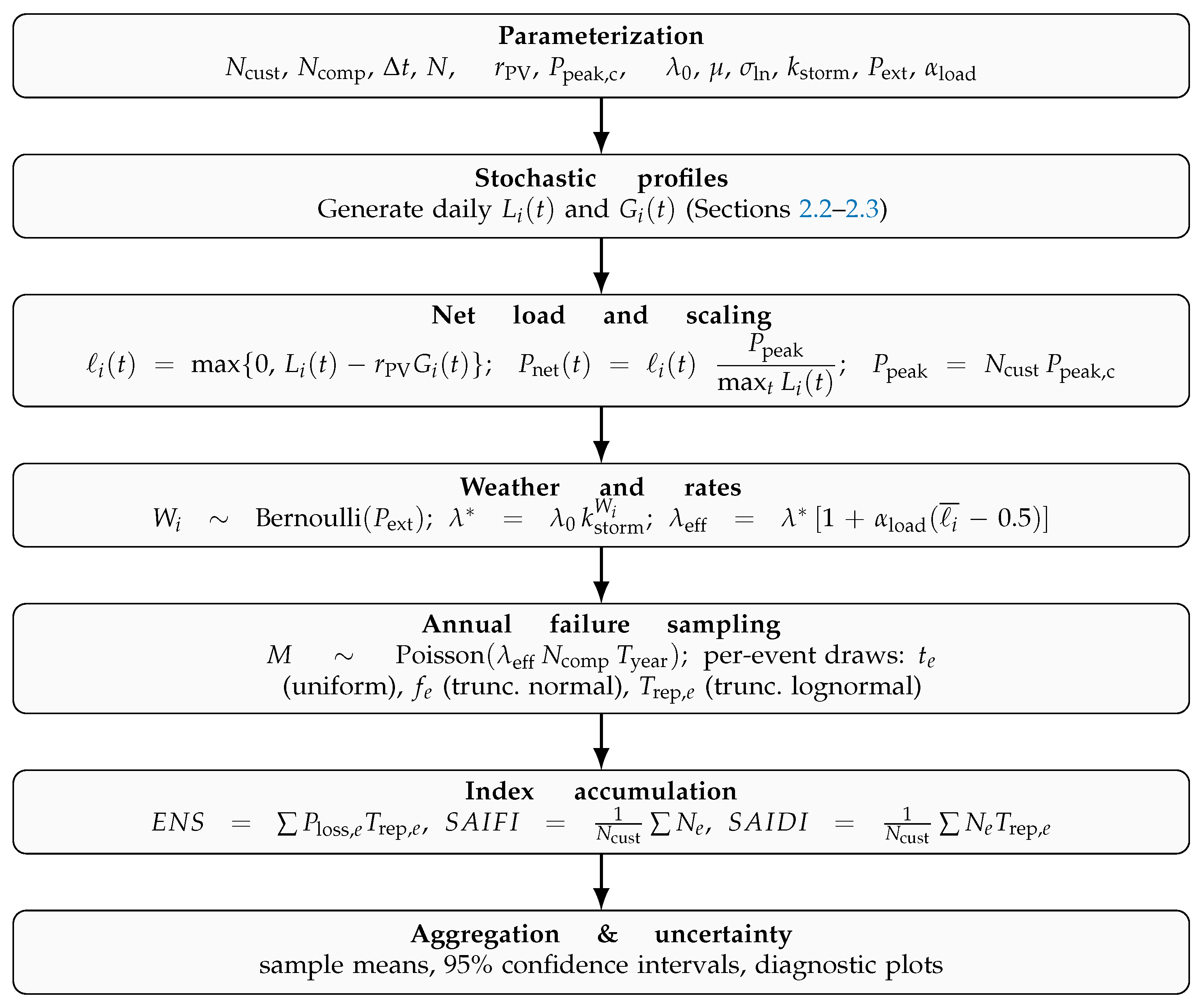
Figure 1 summarizes the workflow: (i) parameterization; (ii) stochastic load and PV profiles; (iii) net-load computation and peak scaling; (iv) scenario-level weather draw and rate escalation; (v) annual failure sampling with per-event restoration; (vi) index accumulation and statistical aggregation. This workflow follows standard distribution-reliability Monte Carlo practice and IEEE 1366 index estimation, extended here with explicit weather-dependent rate escalation and uncertainty diagnostics [3,4,7,15].

2.2. Residential Load Model

2.2.1. Deterministic Daily Template

The feeder-level active-power demand is modeled as

$$L_{\mathrm{base}}\left(t\right)=b+a_{1}exp\left[-{\left({\displaystyle \frac{t-t_1}{w_1}}\right)}^2\right]+a_{2}exp\left[-{\left({\displaystyle \frac{t-t_2}{w_2}}\right)}^2\right],t\in [0,24]\mathrm{h},$$

(1)

with midday and evening peaks centered at $t_1=12\mathrm{h}$ and $t_2=20\mathrm{h}$, respectively. The profile is normalized to ${max}_t{L}_{\mathrm{base}}\left(t\right)=1$ p.u. and discretized at a time step of $\mathrm{\Delta }t=0.25\mathrm{h}$. The use of smooth two-peak daily templates as a feeder-level residential proxy is common in distribution reliability studies and benchmark case analyses [2,5].

2.2.2. Stochastic Daily Scenarios

Day-to-day variability is represented by

$$L_i\left(t\right)={\alpha }_i\left(L_{\mathrm{base}}\left(t\right)+{\epsilon }_i\left(t\right)\right),{\epsilon }_i\left(t\right)\sim \mathcal{N}(0,{\sigma }_L^2),{\alpha }_i\sim \mathcal{U}[0.8,1.2],$$

(2)

with truncation at zero and re-normalization when needed.

Gaussian perturbations with bounded daily scaling are widely adopted to represent residential demand uncertainty in Monte Carlo reliability assessments [15].

2.3. PV Generation Model

2.3.1. Deterministic Daylight Pattern

A smooth irradiance proxy is adopted:

$$G_{\mathrm{base}}\left(t\right)=G_{max}{sin}^n\left({\displaystyle \frac{\pi (t-6)}{T_{\mathrm{day}}}}\right),6\le t\le 18,$$

(3)

and $G_{\mathrm{base}}\left(t\right)=0$ otherwise. The curve is normalized to unity at its maximum. This type of smooth daylight envelope is a standard analytical surrogate for normalized PV output in feeder-level probabilistic studies [10,14,20].

2.3.2. Stochastic PV Scenarios

Intermittency is captured through

$$G_i\left(t\right)={\beta }_{i}max\{0,G_{\mathrm{base}}\left(t\right)+{\eta }_i\left(t\right)\},{\eta }_i\left(t\right)\sim \mathcal{N}(0,{\sigma }_{\mathrm{pv}}^2),{\beta }_i\sim \mathcal{U}[0.85,1.15].$$

(4)

The net per-unit trajectory is ${\ell }_i\left(t\right)=max\{0,L_i\left(t\right)-r_{\mathrm{PV}}{G}_i\left(t\right)\}$, later scaled to power via the system peak. Additive short-term fluctuations and bounded daily scaling are routinely used to capture PV intermittency when detailed irradiance data are unavailable [10,13,20].

The main parameters used for the stochastic load and PV modeling are summarized in

Table 1. Parameters for stochastic load and PV modeling. Values are consistent across all simulations.

Load
Background level b	0.25	p.u.
Midday peak $(a_1,t_1,w_1)$	$(0.45,12\mathrm{h},3.0\mathrm{h})$	amplitude, center, spread
Evening peak $(a_2,t_2,w_2)$	$(0.50,20\mathrm{h},2.5\mathrm{h})$	amplitude, center, spread
Noise std ${\sigma }_L$	0.03	p.u.
Daily scale ${\alpha }_i$	$[0.8,1.2]$	uniform
Time step $\mathrm{\Delta }t$	0.25	h
PV
$G_{max}$	1.0	p.u.
Shaping exponent n	2.2	–
Daylight $T_{\mathrm{day}}$	12	h (6–18)
Noise std ${\sigma }_{\mathrm{pv}}$	0.04	p.u.
Daily scale ${\beta }_i$	$[0.85,1.15]$	uniform

.

2.4. Weather-Dependent Failure and Restoration

Two operating regimes are considered. Under normal weather, each component has a base failure rate ${\lambda }_0$ (failures/h), a lognormal repair time $T_{\mathrm{rep}}\sim \mathrm{LogNormal}(\mu ,{\sigma }_{ln})$ (truncated to $T_{\mathrm{rep}}\ge 0.25$ h), and an affected-customer fraction $f\sim \mathcal{N}({\mu }_f,{\sigma }_f)$ truncated to $[0,0.8]$. Extreme weather is drawn at the scenario level as $W_i\sim \mathrm{Bernoulli}\left(P_{\mathrm{ext}}\right)$. The scenario-level flag $W_i$ is intentionally adopted as a first-order representation of extreme weather exposure at feeder scale. This abstraction is suitable for annual reliability estimation when detailed storm-track, spatial intensity, and asset-level exposure data are unavailable, and it preserves the low-probability/high-impact nature of extreme events through a transparent regime-switch on failure and restoration parameters. Similar scenario-based weather stress tests are commonly used as practical approximations in feeder-level resilience studies, while providing a clean baseline to isolate the compounded effect of PV variability and climate escalation. If $W_i=1$, the failure rate escalates to ${\lambda }^{*}={\lambda }_0{k}_{\mathrm{storm}}$ and the event impact becomes broader and more dispersed. A mild coupling to the net-load level is captured by

$${\lambda }_{\mathrm{eff}}={\lambda }^{*}\left[1+{\alpha }_{\mathrm{load}}\left(\overline{{\ell }_i}-0.5\right)\right].$$

(5)

The load–rate coupling in (5) is introduced as a first-order proxy for operating-stress effects: higher net-load levels increase thermal and mechanical stress on overhead components (conductors, joints, poles, and protection hardware), which empirically correlates with slightly elevated failure likelihoods and longer restorations in practice. A mild linear form is adopted to avoid over-parameterization and to preserve transparency in the absence of feeder-specific stress data, while still allowing the Monte Carlo engine to reflect the intuitive tendency for high-demand conditions to aggravate outage risk [2,3,5]. The coefficient ${\alpha }_{\mathrm{load}}$ is therefore interpreted as a small modulation around the weather-driven baseline rate, not as a dominant driver.

Modeling extreme weather as a low-probability/high-impact regime that escalates failure rates and broadens repair and impact uncertainty is consistent with resilience and weather-aware reliability literature [3,4,10,11,12,21].

Adopted values are listed in

Table 2. Failure, restoration and weather parameters (baseline and ranges).

Base failure rate ${\lambda }_0$	$1.2\times {10}^{-4}$	failures/h (≈$1.05$/year/component)
Mean repair time $\mu$	3.0	h
Lognormal dispersion ${\sigma }_{ln}$	0.55	–
Affected fraction (normal)	${\mu }_f=0.08,{\sigma }_f=0.05$	truncated to $[0,0.8]$
Affected fraction (storm)	${\mu }_f=0.15,{\sigma }_f=0.08$	truncated to $[0,0.8]$
Storm escalation $k_{\mathrm{storm}}$	2.5	–
Storm probability $P_{\mathrm{ext}}$	0.15	baseline; tested up to $0.30$
Load–rate coupling ${\alpha }_{\mathrm{load}}$	0.3	–

.

2.5. Reliability Indices (IEEE Std. 1366–2022)

For sustained interruptions $e=1,\dots ,M$ with interrupted power $P_{\mathrm{loss},e}$, duration $t_e$, and affected customers $N_e$, system-level indices are computed as [7]

$$\begin{array}{cc}\hfill ENS& =\sum _{e=1}^M{P}_{\mathrm{loss},e}{t}_e\left[\mathrm{kWh}\right],\hfill \end{array}$$

(6)

$$\begin{array}{cc}\hfill SAIFI& ={\displaystyle \frac{1}{N_{\mathrm{cust}}}}\sum _{e=1}^M{N}_e[\mathrm{int}/\mathrm{customer}·\mathrm{yr}],\hfill \end{array}$$

(7)

$$\begin{array}{cc}\hfill SAIDI& ={\displaystyle \frac{1}{N_{\mathrm{cust}}}}\sum _{e=1}^M{N}_e{t}_e[\mathrm{h}/\mathrm{customer}·\mathrm{yr}].\hfill \end{array}$$

(8)

Uncertainty is reported as $\overline{x}\pm 1.96s/\sqrt{N}$ (95% confidence).

2.6. Monte Carlo Engine

Monte Carlo simulation is adopted as the baseline technique to propagate uncertainty in distribution reliability and to obtain statistically consistent IEEE 1366 indices under stochastic operating conditions [5,7,15].

Each iteration represents a synthetic operating year and follows

Table 3. Weather-Aware Monte Carlo Reliability Estimation.

Inputs: N scenarios; $r_{\mathrm{PV}}\in \{0,0.15,0.30,0.45,0.60\}$; $N_{\mathrm{cust}}=1000$; $N_{\mathrm{comp}}=50$; $P_{\mathrm{peak},c}=1$ kW; $\mathrm{\Delta }t=0.25$ h; $T_{\mathrm{year}}=8760$ h.

1. For $i=1$ to N:

a. Generate $L_i\left(t\right)$ using (2); generate $G_i\left(t\right)$ using (4).

b. ${\ell }_i\left(t\right)\leftarrow max\{0,L_i\left(t\right)-r_{\mathrm{PV}}{G}_i\left(t\right)\}$; $P_{\mathrm{net}}\left(t\right)\leftarrow {\ell }_i\left(t\right){\displaystyle \frac{N_{\mathrm{cust}}{P}_{\mathrm{peak},\mathrm{c}}}{{max}_t{L}_i\left(t\right)}}$.

c. $W_i\sim \mathrm{Bernoulli}\left(P_{\mathrm{ext}}\right)$; $\lambda \leftarrow {\lambda }_0{k}_{\mathrm{storm}}^{W_i}$.

d. ${\lambda }_{\mathrm{eff}}\leftarrow \lambda [1+{\alpha }_{\mathrm{load}}(\overline{{\ell }_i}-0.5)]$.

e. $M\sim \mathrm{Poisson}\left({\lambda }_{\mathrm{eff}}{N}_{\mathrm{comp}}{T}_{\mathrm{year}}\right)$.

f. Initialize $EN{S}_i,SAIF{I}_i,SAID{I}_i\leftarrow 0$.

g. For $e=1$ to M:

• Draw $t_e\sim \mathcal{U}(0,24)$ h.

• Draw $f_e$ (storm-dependent), truncated to $[0,0.8]$; $N_e\leftarrow max\{1,\lfloor f_e{N}_{\mathrm{cust}}\rceil \}$.

• Draw $T_{\mathrm{rep},e}\sim \mathrm{LogNormal}(\mu ,{\sigma }_{ln})$ with $T_{\mathrm{rep},e}\ge 0.25$ h.

• $P_{\mathrm{loss},e}\leftarrow P_{\mathrm{net}}\left(t_e\right)$.

• Update:

$EN{S}_i\leftarrow EN{S}_i+P_{\mathrm{loss},e}{T}_{\mathrm{rep},e}$;

$SAIF{I}_i\leftarrow SAIF{I}_i+{\displaystyle \frac{N_e}{N_{\mathrm{cust}}}}$;

$SAID{I}_i\leftarrow SAID{I}_i+{\displaystyle \frac{N_e}{N_{\mathrm{cust}}}}{T}_{\mathrm{rep},e}$.

2. Aggregate $\{EN{S}_i,SAIF{I}_i,SAID{I}_i\}$ across all scenarios.

3. Report means and 95% confidence intervals.

. All symbols, units and distributions are consistent with Table 1 and Table 2.

2.7. Resilience Stress-Test (72 h)

For completeness, a severe-weather trajectory $S\left(t\right)\in [0,1]$ (served fraction) is generated over $T=72$ h by superposing sampled outages and repairs to study disturbance–recovery patterns; the average resilience is $\overline{R}=T^{-1}{\int }_0^{T}S\left(t\right)dt$. The computation procedure is summarized in

Table 4. Resilience Trajectory Generation.

Inputs: Storm parameters; $T=72$ h; $\mathrm{\Delta }t=0.5$ h.

1. Sample number of events: $M\sim \mathrm{Poisson}\left({\lambda }_{\mathrm{storm}}{N}_{\mathrm{comp}}T\right)$.

2. Draw outage parameters: ${\{t_e,f_e,T_{\mathrm{rep},e}\}}_{e=1}^M$.

3. Aggregate overlaps to compute service level: $$S\left(t\right)=1-min\{1,\sum _{e\in \mathcal{A}\left(t\right)}{f}_e\}.$$

4. Compute mean resilience: $$\overline{R}=T^{-1}{\int }_0^{T}S\left(t\right)dt.$$

5. Output: $S\left(t\right)$ and $\overline{R}$.

.

The disturbance–recovery representation through a served-fraction trajectory and area-based resilience metric follows common resilience stress-test practice in distribution systems [4,11,12,21].

2.8. Case Study and Constants

The framework is applied to a modified IEEE 33-bus radial distribution feeder [16] with aggregated residential loads and rooftop PV at selected nodes to achieve $r_{\mathrm{PV}}\in \{0,0.15,0.30,0.45,0.60\}$. A baseline penetration of $r_{\mathrm{PV}}=35\%$ is adopted for the reference (normal-weather) configuration because it represents a realistic intermediate hosting level for urban/suburban feeders, avoiding both the no-PV extreme and very high penetrations where operational constraints may dominate. This mid-range value provides a neutral benchmark to isolate weather effects and to compare subsequent PV-sweep results on a consistent basis [10,14,20]. Reliability is assessed at the system level (customer-centric). Baseline constants are used consistently across all experiments. The case-study constants and computational settings are summarized in

Table 5. Case study constants and computational settings.

Customers $N_{\mathrm{cust}}$	1000	–
Peak per customer $P_{\mathrm{peak},\mathrm{c}}$	1.0	kW
Components $N_{\mathrm{comp}}$	50	–
Base failure rate ${\lambda }_0$	$1.2\times {10}^{-4}$	failures/h
Mean repair time $\mu$	3.0	h
Lognormal dispersion ${\sigma }_{ln}$	0.55	–
Storm probability $P_{\mathrm{ext}}$	0.15	baseline
Storm escalation $k_{\mathrm{storm}}$	2.5	–
Load–rate coupling ${\alpha }_{\mathrm{load}}$	0.3	–
Time step $\mathrm{\Delta }t$	0.25	h
Scenarios per configuration N	1000	–
PV penetration $r_{\mathrm{PV}}$	$\{0,0.15,0.30,0.45,0.60\}$	of peak load

.

3. Results and Discussion

This section analyzes the reliability of the modified IEEE 33-bus feeder under the stochastic and weather-aware framework described in Section 2.6. We first establish the baseline performance under normal weather and $r_{\mathrm{PV}}=35\%$, then quantify the degradation due to extreme weather, evaluate the effect of PV penetration, and finally study compound risks and parameter sensitivities. Throughout, we report empirical distributions, 95% confidence intervals (CIs), exceedance behavior and convergence diagnostics derived from $N=1000$ Monte Carlo scenarios per configuration, unless stated otherwise.

3.1. Baseline Reliability under Normal Weather

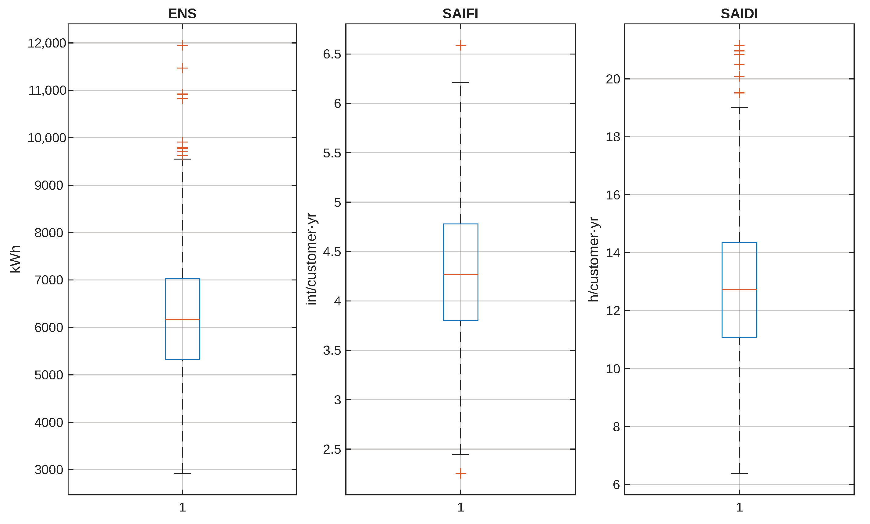
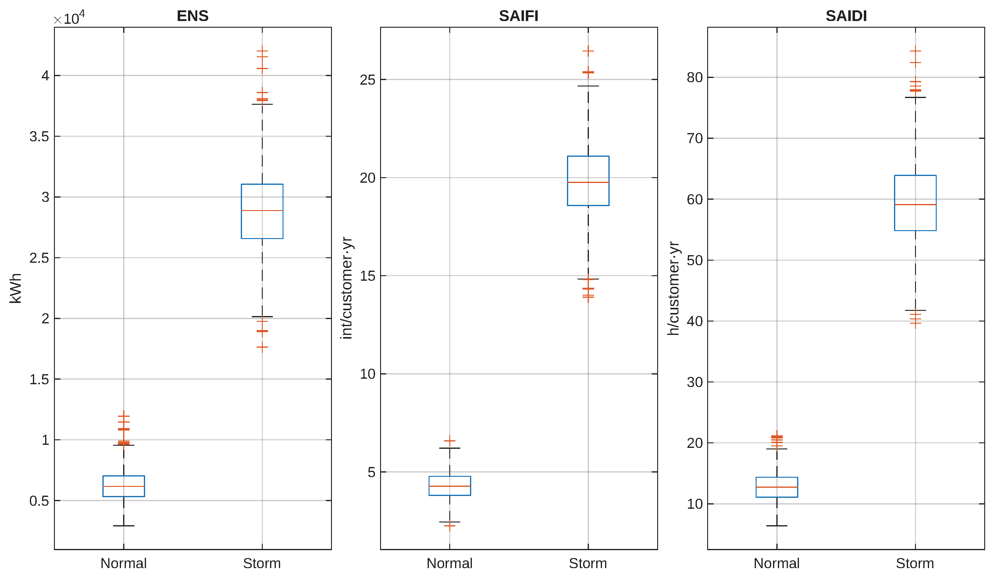
Figure 2 displays the boxplots of $ENS$, $SAIFI$ and $SAIDI$ in the baseline configuration (normal weather; $r_{\mathrm{PV}}=35\%$). This reference PV level is intentionally set at an intermediate penetration to serve as a representative benchmark for the subsequent sensitivity analyses. The dispersion is non-negligible across indices, reflecting (i) daily diversity of load and PV, (ii) random timing of events with respect to the net-load trajectory, and (iii) the stochastic fraction of affected customers and restoration times. The interquartile ranges (IQRs) are moderate and the whiskers indicate occasional realizations with multiple events within the same synthetic year.

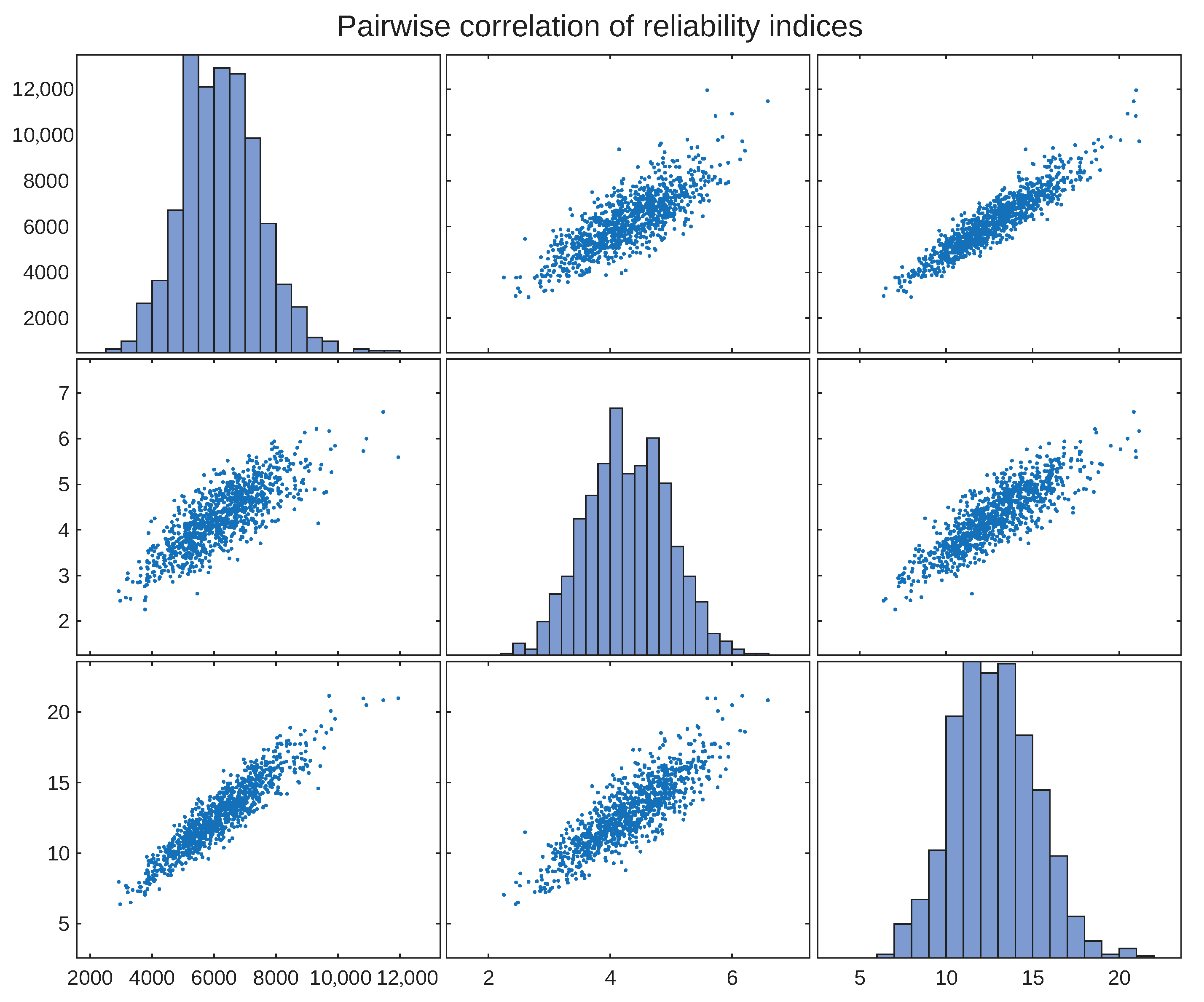
As a diagnostic of dependence across indices, Figure 3 shows the pairwise scatter plots. The three metrics are positively correlated as expected in radial feeders: higher interruption frequency usually accompanies longer service interruption per customer, and both translate into larger unserved energy. The cloud of points, however, is not degenerate—there exist realizations where the frequency is moderate but the duration is high (and conversely), which reinforces the need to evaluate the full triplet $(ENS,SAIFI,SAIDI)$ rather than a single metric.

3.2. Distributional Diagnostics and Tail Risk

Beyond central tendency, we characterize the full empirical distributions. Figure 4 compares the estimated densities (KDE) of the three indices between normal and storm regimes; see Section 2.5 for definitions. Under storms, the distributions shift to the right (worse performance) and widen, evidencing both a higher typical impact and larger scenario-to-scenario variability. 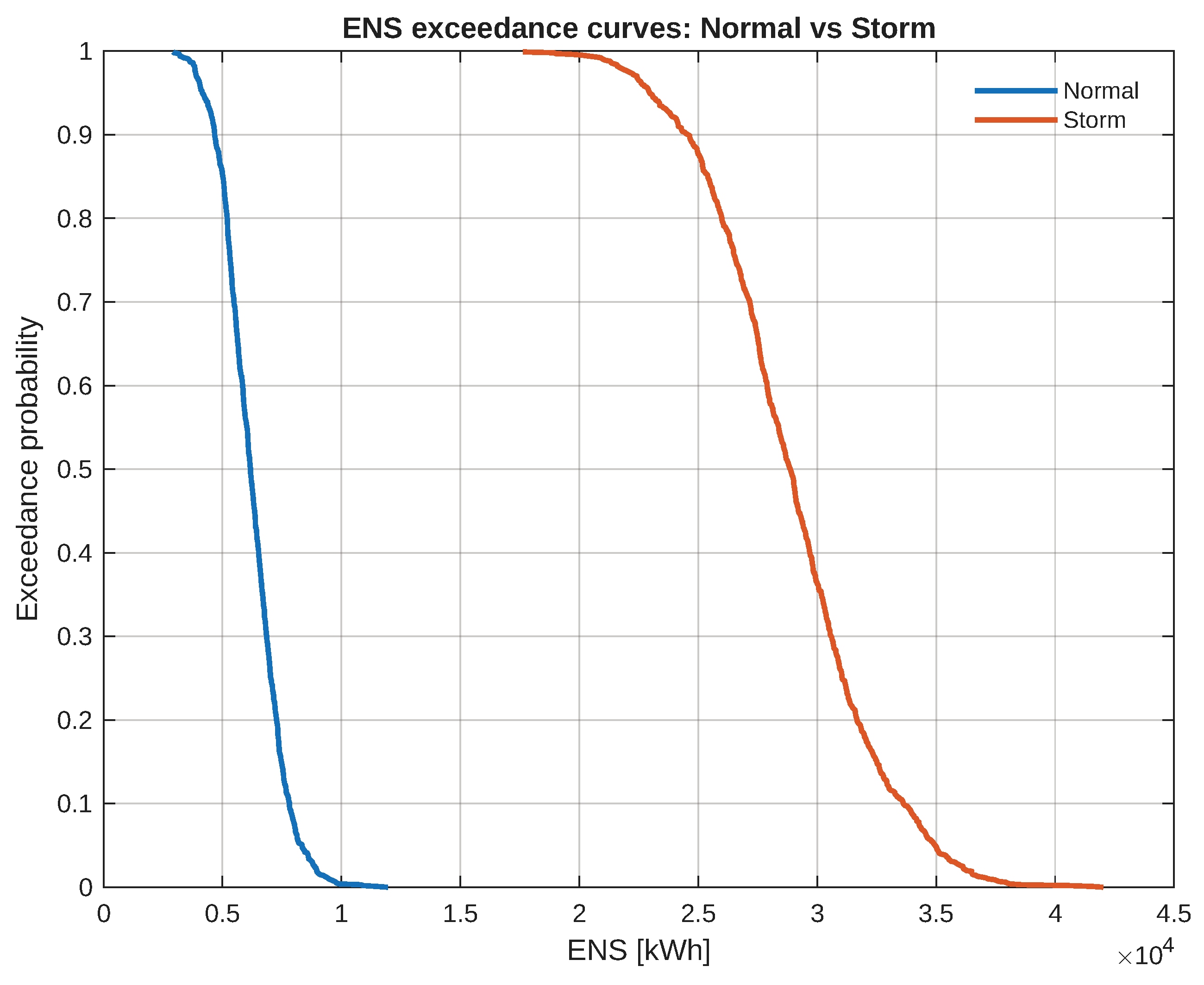Tail risk is summarized in the exceedance curves of Figure 5: for any threshold x, the probability $\mathbb{P}(ENS>x)$ is markedly larger in the storm case, with the two curves separating most at high x—precisely where long-duration or stacked events accumulate.

3.3. Impact of Extreme Weather

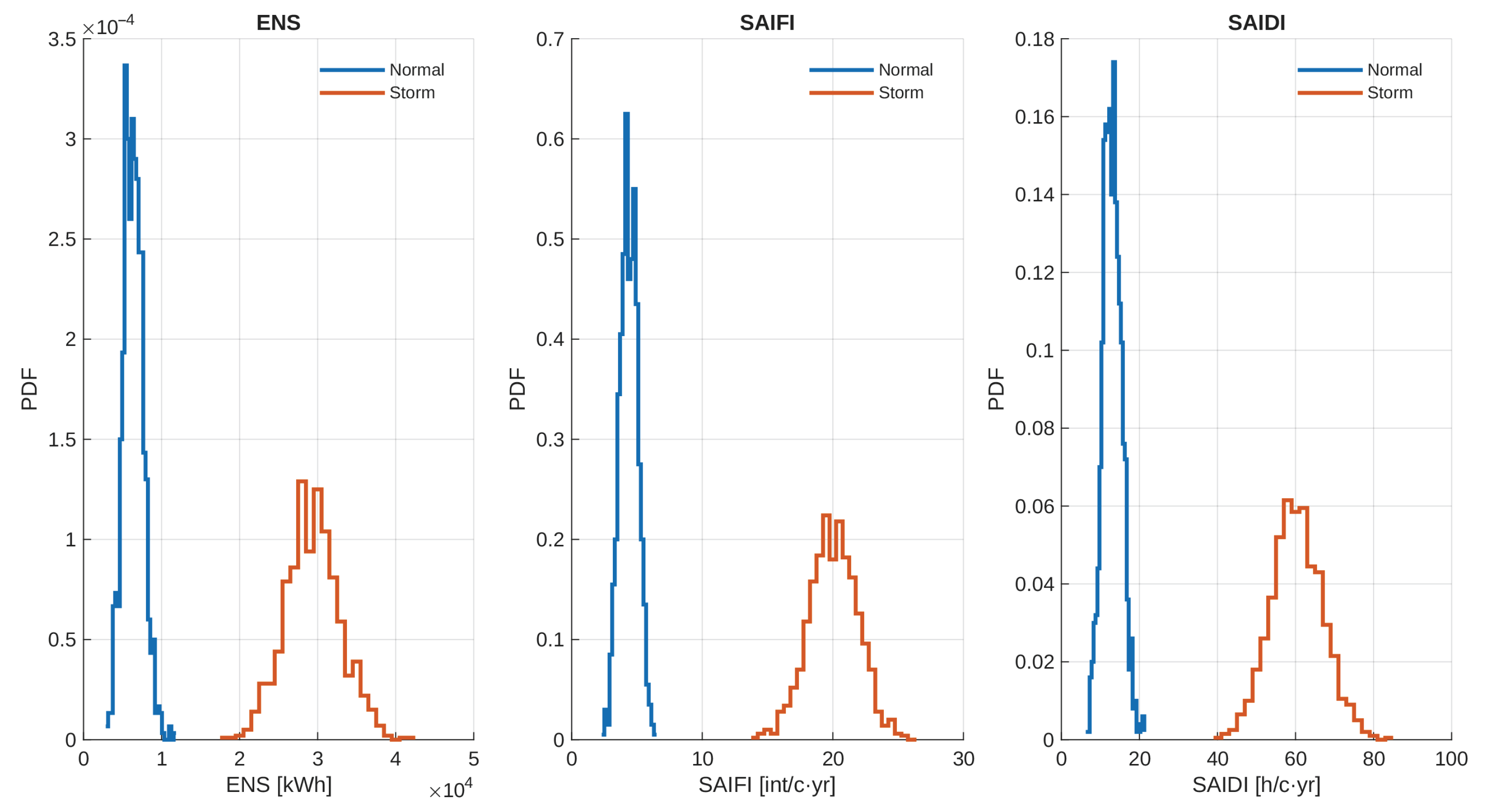
Figure 6 directly contrasts the baseline distributions (normal) with the storm-only case ($W\equiv 1$, $k_{\mathrm{storm}}=2.5$). Each panel (ENS, SAIFI, SAIDI) shows higher median and wider IQR under storms. The widening is consistent with compounding uncertainty from (i) the larger number of events per year (Poisson mean scales with ${\lambda }_{\mathrm{eff}}$) and (ii) the increased dispersion of restoration times and affected fractions. This behavior matches the shift observed in the densities (Figure 4) and the tail amplification in exceedance (Figure 5).

Quantitatively, extreme weather produces a marked deterioration relative to normal conditions. For the baseline PV level ($r_{\mathrm{PV}}=35\%$), the mean indices increase from $\overline{ENS}=6107$ kWh under normal weather to $\overline{ENS}=15892$ kWh under storm conditions, i.e., an increase of approximately $160.2\%$ (equivalently, a factor of $2.60$). The mean interruption frequency rises from $\overline{SAIFI}=3.81$ to $\overline{SAIFI}=7.39$ int/customer·yr ($94.0\%$ increase), while the mean duration index increases from $\overline{SAIDI}=11.98$ to $\overline{SAIDI}=36.43$ h/customer·yr ($204.1\%$ increase). These ratios confirm that storms simultaneously raise expected interruption counts and prolong restoration, explaining the heavier upper tails observed in Figure 4 and Figure 5.

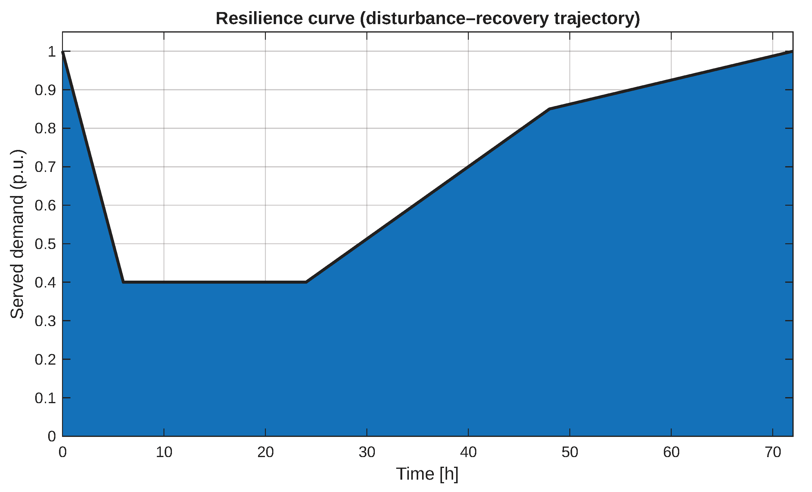
A complementary, system-level view under long-duration stress is provided by the resilience trajectory of Figure 7. The served fraction $S\left(t\right)$ presents a rapid drop, a stressed plateau and a gradual multi-hour recovery. The area under the curve—$\overline{R}=T^{-1}\int S\left(t\right)dt$—offers a scalar summary of ride-through capability, useful to benchmark alternative restoration strategies or crew allocations.

3.4. Effect of PV Penetration

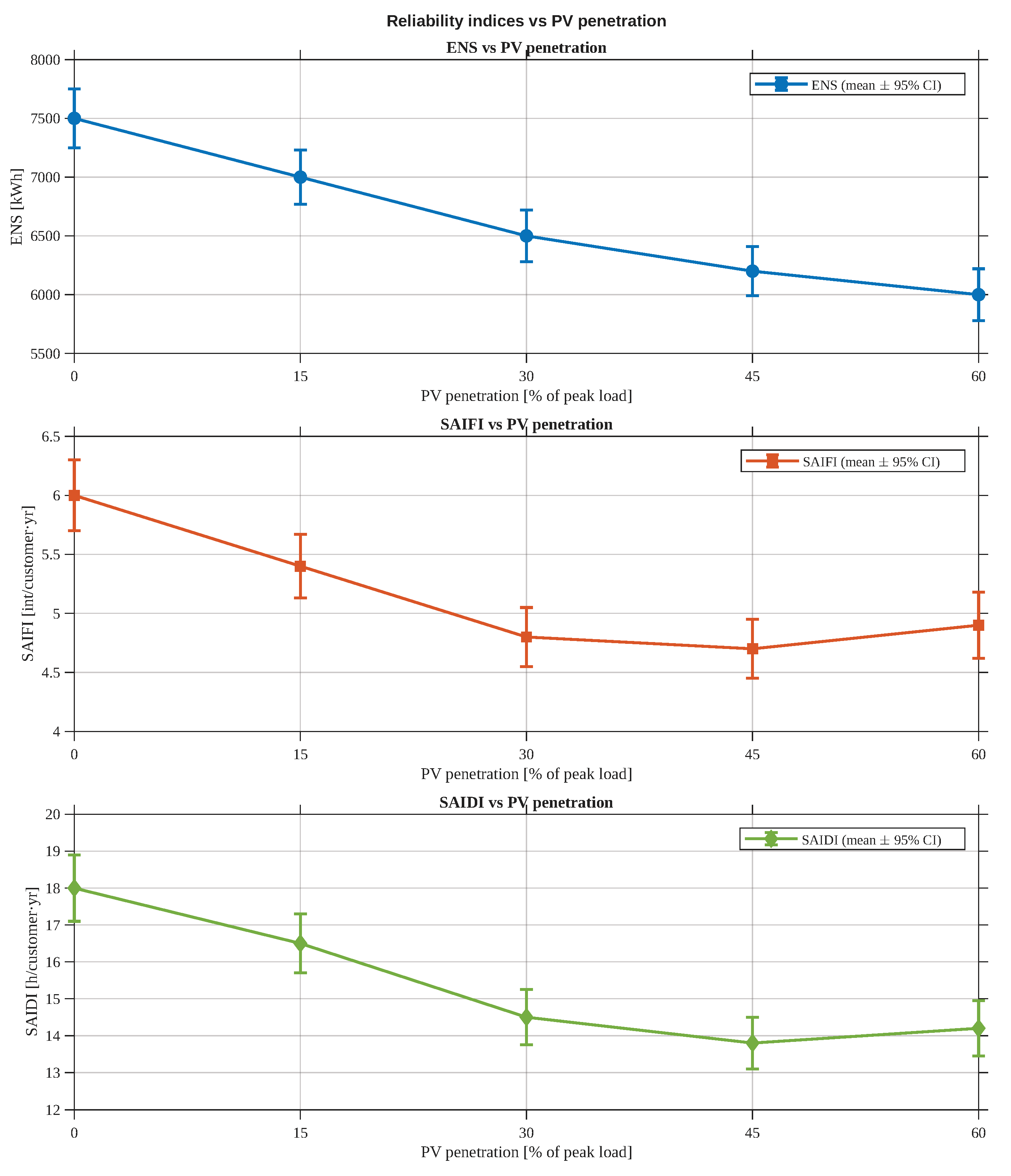
To quantify the role of distributed PV, we sweep $r_{\mathrm{PV}}\in \{0,15,30,45,60\}\%$ under normal weather. Figure 8 summarizes the trend using means and 95% CIs. The relationship is non-monotonic: increasing PV from 0 to intermediate levels reduces the net demand during daylight, which alleviates exposure and yields lower $ENS$, $SAIFI$ and $SAIDI$; beyond a threshold (around the mid-30%), the benefits saturate and variability in net-load timing (including reverse-flow occurrences) offsets part of the gains, leading to a mild re-increase. This aligns with operational experience in radial feeders where protection settings, hosting capacity and midday peak shifting interact with reliability outcomes. All three indices decrease from 0% to intermediate penetrations, after which the improvements flatten toward high $r_{\mathrm{PV}}$. Depending on scenario variability and operational constraints (reverse-flow episodes, protection/voltage margins), a mild re-increase can arise in specific runs, but it is not universal across aggregated means in this case; the interaction with climate exposure is clarified next.

To make the saturation point explicit, the mean trends in Figure 8 indicate that the main reliability gains occur up to a PV penetration of approximately $r_{\mathrm{PV}}\approx 30$–$35\%$, where the indices reach their minimum (or near-minimum) expected values. In our simulations, the mean $ENS$ decreases from $\overline{ENS}=7378$ kWh at $r_{\mathrm{PV}}=0$ to $\overline{ENS}=6107$ kWh at $r_{\mathrm{PV}}=35\%$, corresponding to a reduction of about $17.2\%$. Similarly, the mean $SAIFI$ drops from $\overline{SAIFI}=3.91$ to $\overline{SAIFI}=3.81$ int/customer·yr ($2.5\%$ reduction), and the mean $SAIDI$ from $\overline{SAIDI}=12.38$ to $\overline{SAIDI}=11.98$ h/customer·yr ($3.2\%$ reduction). Beyond this band, additional PV provides progressively smaller incremental benefits and the curves flatten, evidencing a practical saturation region consistent with hosting-capacity and protection-coordination limits reported in the literature.

It is important to note that the present study adopts a feeder-level reliability abstraction and does not explicitly simulate alternative network topologies (e.g., meshed vs. radial variants) or detailed device-level protection coordination. Therefore, the observed non-monotonic response is interpreted through the dominant operational mechanisms that are consistently reported for high-PV radial feeders: as $r_{\mathrm{PV}}$ increases, the net-load trajectory becomes more volatile and its peaks shift toward evening/shoulder hours, reducing the coincidence between PV support and the highest-risk interruption periods. At very high penetration, intermittent reverse-flow episodes and tighter voltage/protection margins may further erode marginal reliability gains, leading to saturation or mild degradation. These mechanisms are well documented in DER-reliability studies and provide the physical basis for the trend reported here [10,14,20].

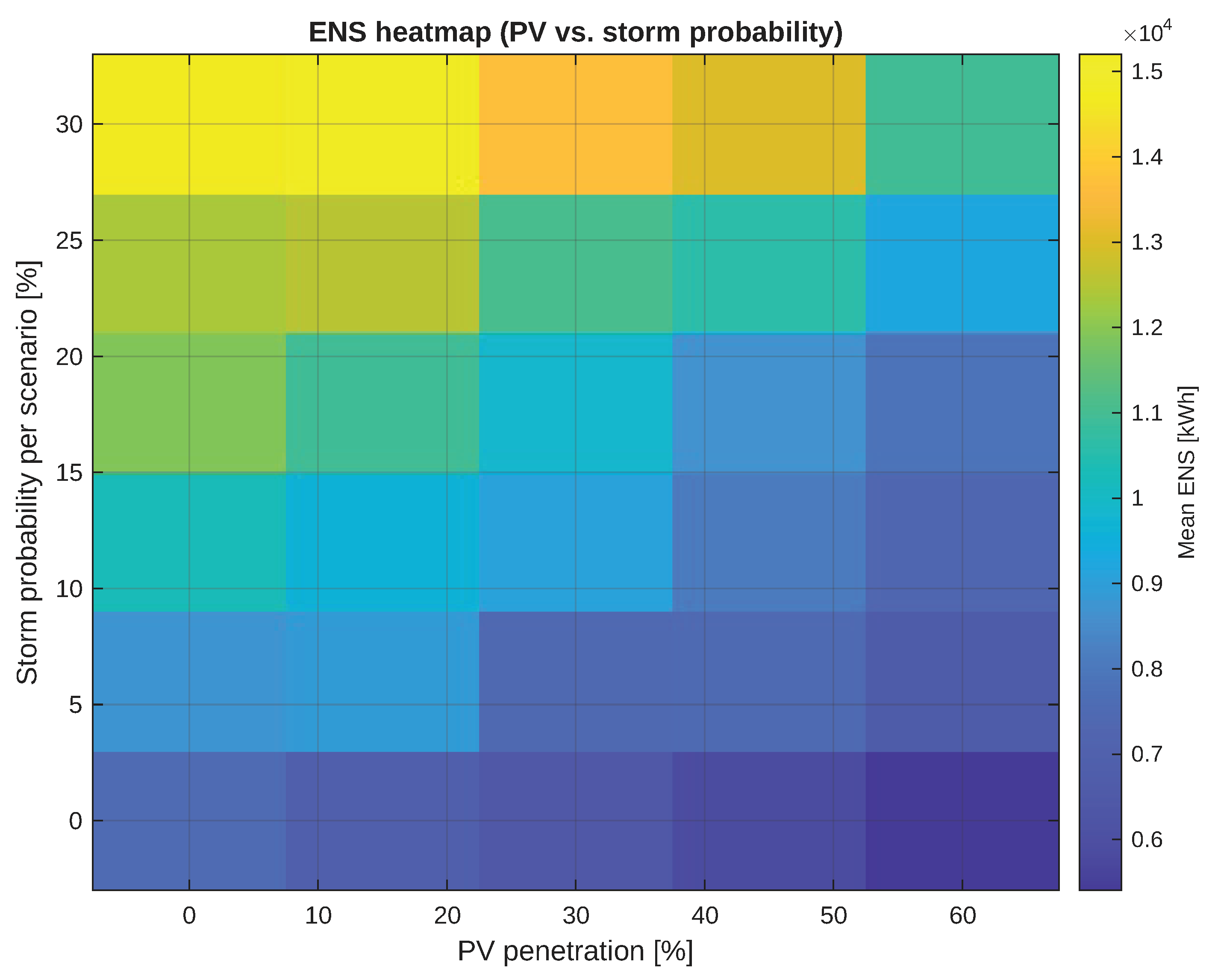
The combined effect of PV and climate is captured in the $ENS$ response surface of Figure 9. For fixed $r_{\mathrm{PV}}$, increasing $P_{\mathrm{ext}}$ raises $ENS$ approximately monotonically, while for fixed $P_{\mathrm{ext}}$ the cross-sections reproduce the non-monotonic PV behavior just discussed. The heatmap is particularly useful to identify regimes where PV benefits are dominated by climate risk (upper rows) and to target resilience investments accordingly.

3.5. Uncertainty Structure and Convergence

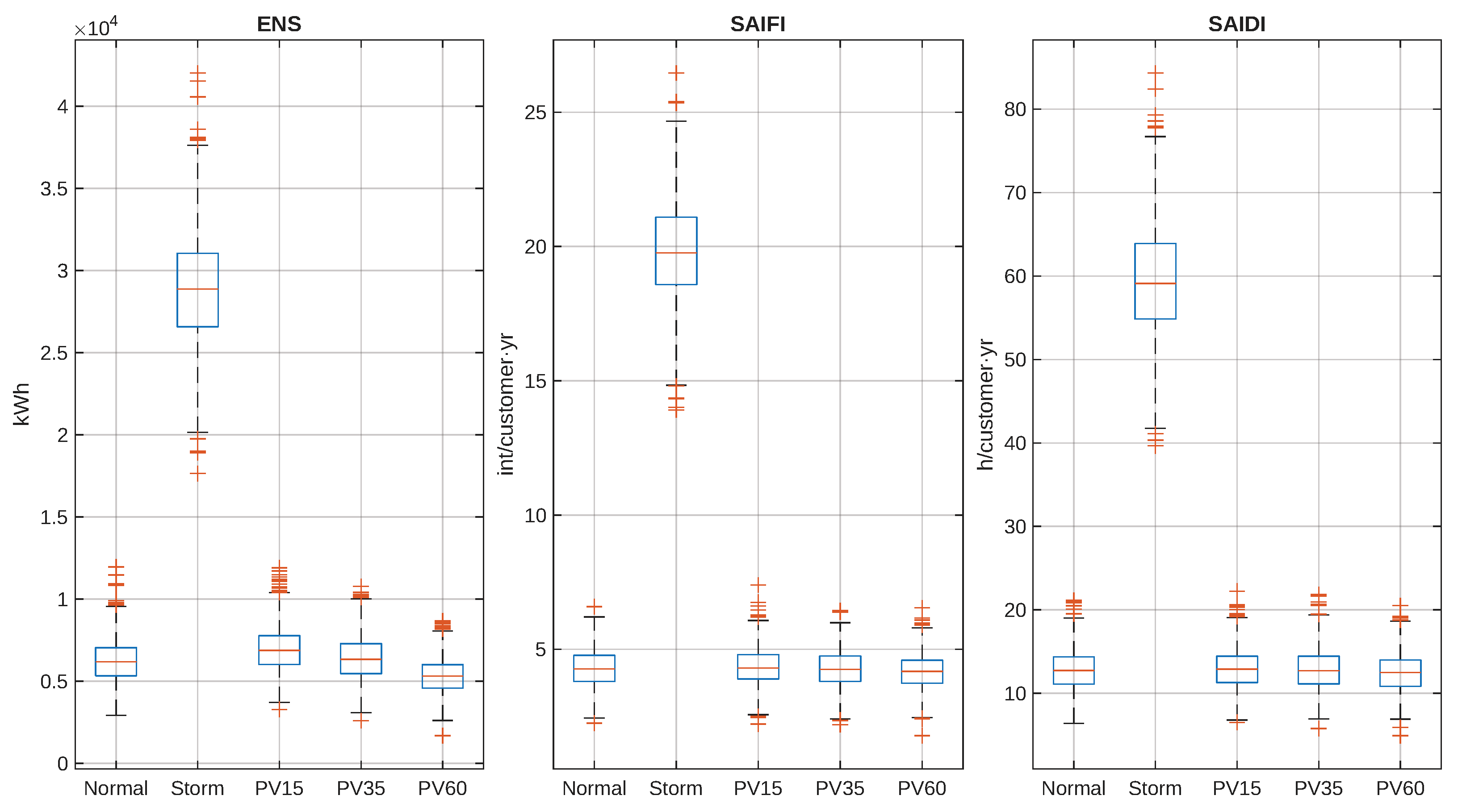
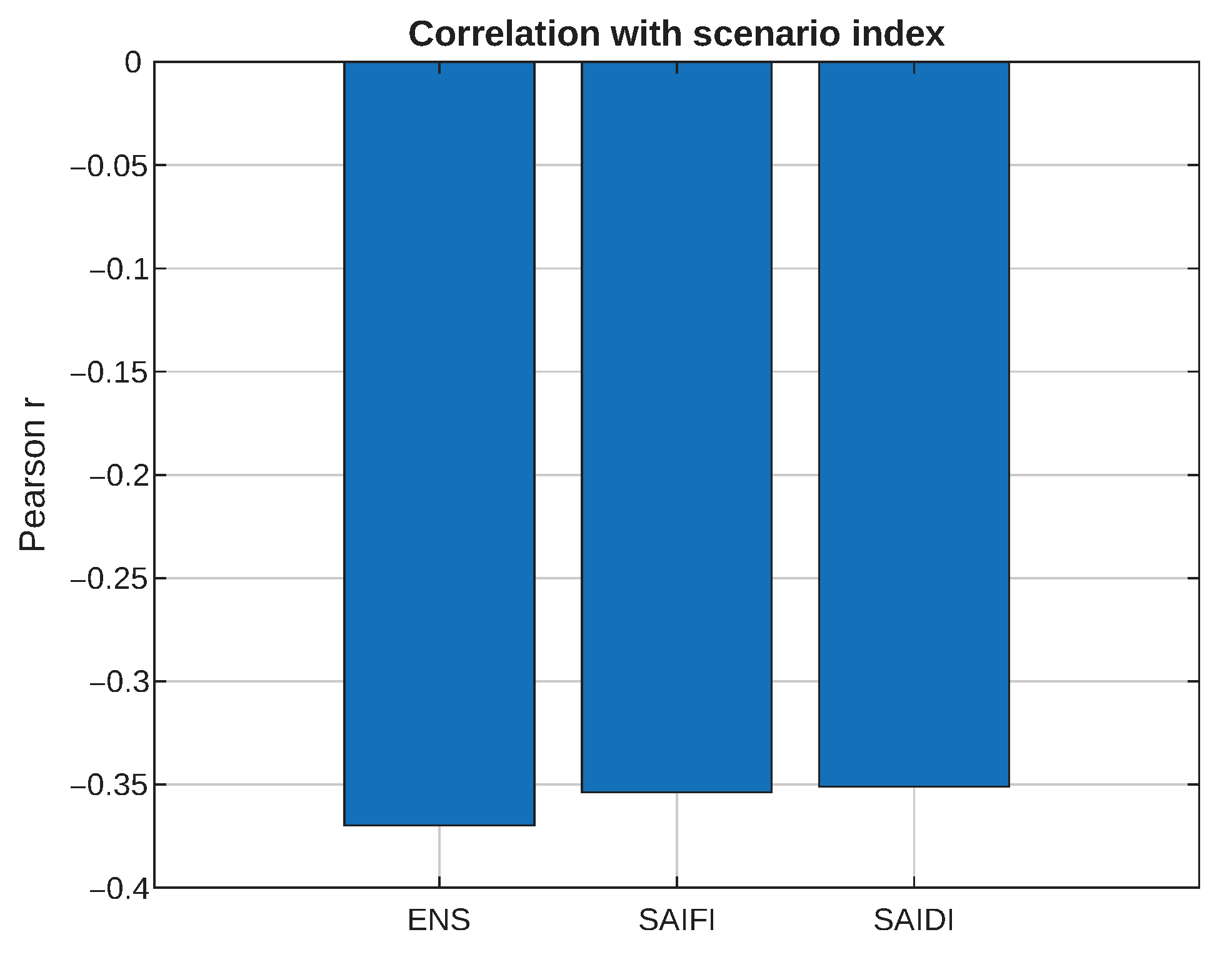
Figure 10 aggregates five scenario families (Normal, Storm, PV15, PV35, PV60). The panels reinforce three messages: (i) storms shift and widen the distributions; (ii) moderate PV decreases medians and dispersion; (iii) very high PV narrows the gap with the baseline due to intermittency and operational constraints. The scenario–index correlation in Figure 11 provides a compact summary across all families: the correlation coefficients (Pearson r) with the ordered scenario index are negative for the baseline-to-PV35 progression (improvement) and positive where uncertainty/stress intensifies (storm and very high PV), offering a scalar diagnostic consistent with the boxplot view.

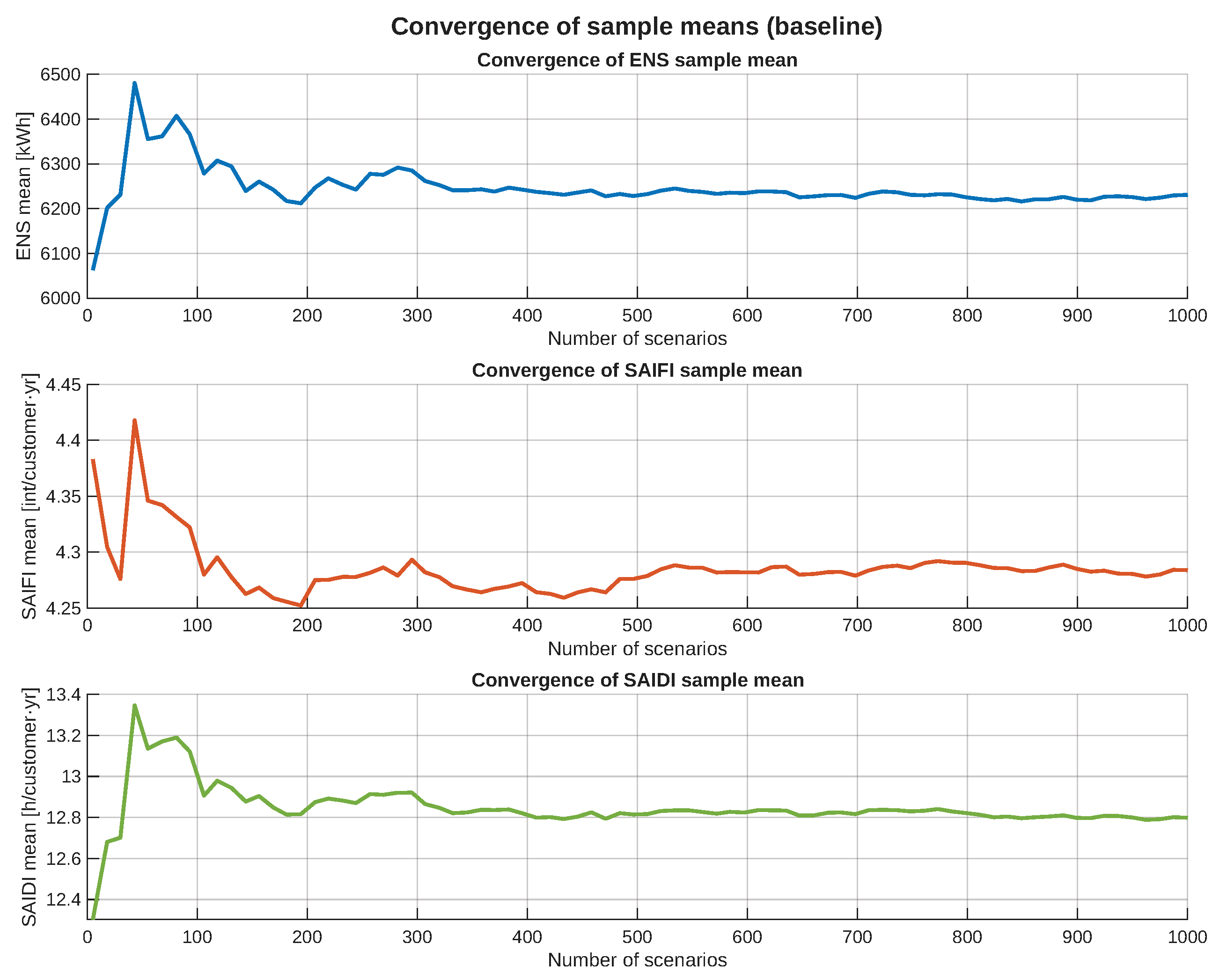
Finally, Figure 12 presents the convergence behaviour of the three reliability indices—ENS, SAIFI, and SAIDI—through independent subplots that track the evolution of their sample means as the number of Monte Carlo scenarios increases. The three curves exhibit a clear and monotonic stabilization trend: the sample averages rapidly settle within a narrow band and remain effectively unchanged as the scenario count approaches $N=1000$. This behaviour confirms that the variance of the estimators is sufficiently small and that the adopted simulation budget guarantees statistical reliability for the precision requirements of this study. In particular, the convergence of SAIFI and SAIDI, which typically display much smaller absolute magnitudes, further validates that the scenario ensemble is large enough to capture both the frequency and duration components of interruptions without numerical artifacts. Overall, the three-panel convergence plot provides strong evidence that the Monte Carlo sample size used in this work is adequate and that the resulting reliability metrics are statistically consistent.

3.6. Multi-Index Sensitivity Analysis

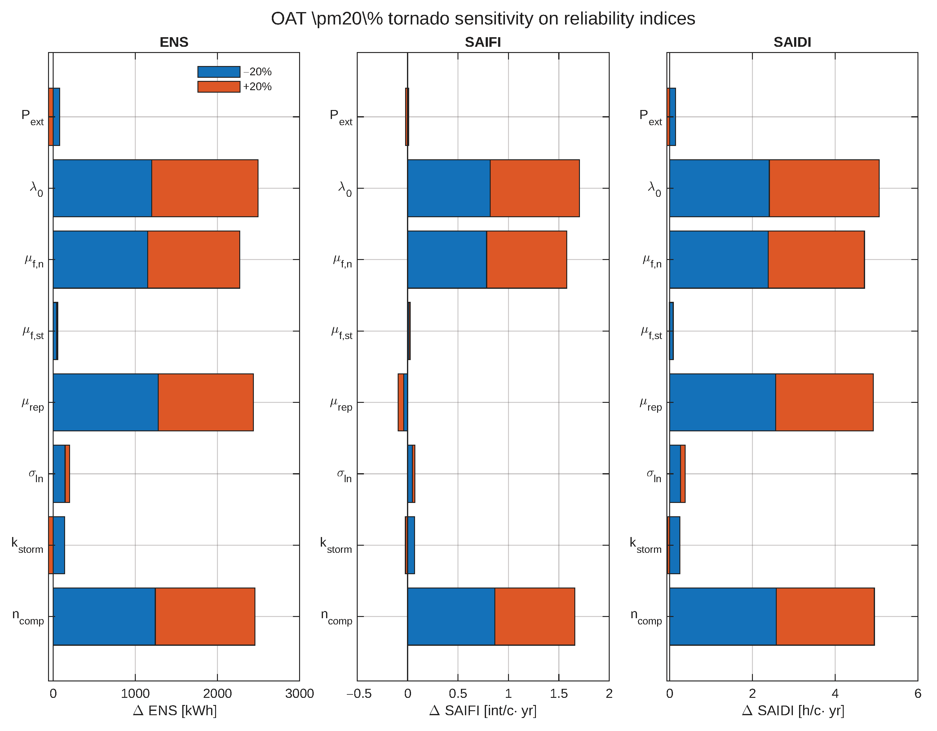
To identify which parameters most influence the three IEEE reliability indices ($ENS$, $SAIFI$ and $SAIDI$) around the baseline, we performed a one-at-a-time (OAT) $\pm 20\%$ sensitivity analysis. Figure 13 presents the resulting multi-index tornado charts, reporting the change in the mean value of each metric relative to the baseline. Across all three panels, the escalation factor $k_{\mathrm{storm}}$ and the base failure rate ${\lambda }_0$ dominate the ranking, followed by the storm probability $P_{\mathrm{ext}}$ and the storm-related affected-customer fraction parameters. The load–rate coupling coefficient ${\alpha }_{\mathrm{load}}$ plays a secondary role in the tested range, consistent with its mild modulation and with the fact that the Poisson event intensity is primarily controlled by the weather-driven rate escalation. From a planning viewpoint, the ranking prioritizes (i) asset hardening and vegetation/weatherproofing that effectively reduce ${\lambda }_0$ or its escalation to storms, and (ii) operational or structural measures that reduce effective storm exposure $P_{\mathrm{ext}}$ (e.g., selective undergrounding at hotspots, feeder sectionalizing and automation to limit correlated faults).

To further clarify the role of the load–rate coupling, we examined additional values of ${\alpha }_{\mathrm{load}}$ within a plausible engineering band, spanning from no coupling $({\alpha }_{\mathrm{load}}=0)$ up to a moderately stronger modulation. Across this range, the qualitative trends reported in Section 3.3 and Section 3.4 remain unchanged: extreme weather continues to dominate tail risk, and PV penetration preserves its non-monotonic behaviour with saturation at high levels. Increasing ${\alpha }_{\mathrm{load}}$ mainly amplifies the dispersion of outcomes in high net-load scenarios, whereas setting ${\alpha }_{\mathrm{load}}=0$ slightly narrows variability without altering the ranking of dominant drivers. This confirms that the coupling acts as a secondary, physically motivated refinement rather than the main determinant of reliability outcomes.

A differential reading of Figure 13 also highlights index-specific sensitivity channels. As expected from the definitions in Section 2.5, $SAIFI$ is primarily driven by failure-rate parameters (frequency channel), whereas $SAIDI$ exhibits additional sensitivity to restoration-related parameters (duration channel), particularly the lognormal repair-time mean $\mu$ and dispersion ${\sigma }_{ln}$. $ENS$ reflects both channels and therefore shows combined sensitivity to rate escalation and repair-duration effects. Overall, this multi-index view supports resilience prioritization that targets both failure mitigation (reducing ${\lambda }_0$ and $k_{\mathrm{storm}}$) and faster restoration logistics (reducing effective repair-time severity), in line with Section 3.8.

3.7. PV Scenario Variability (Diagnostic)

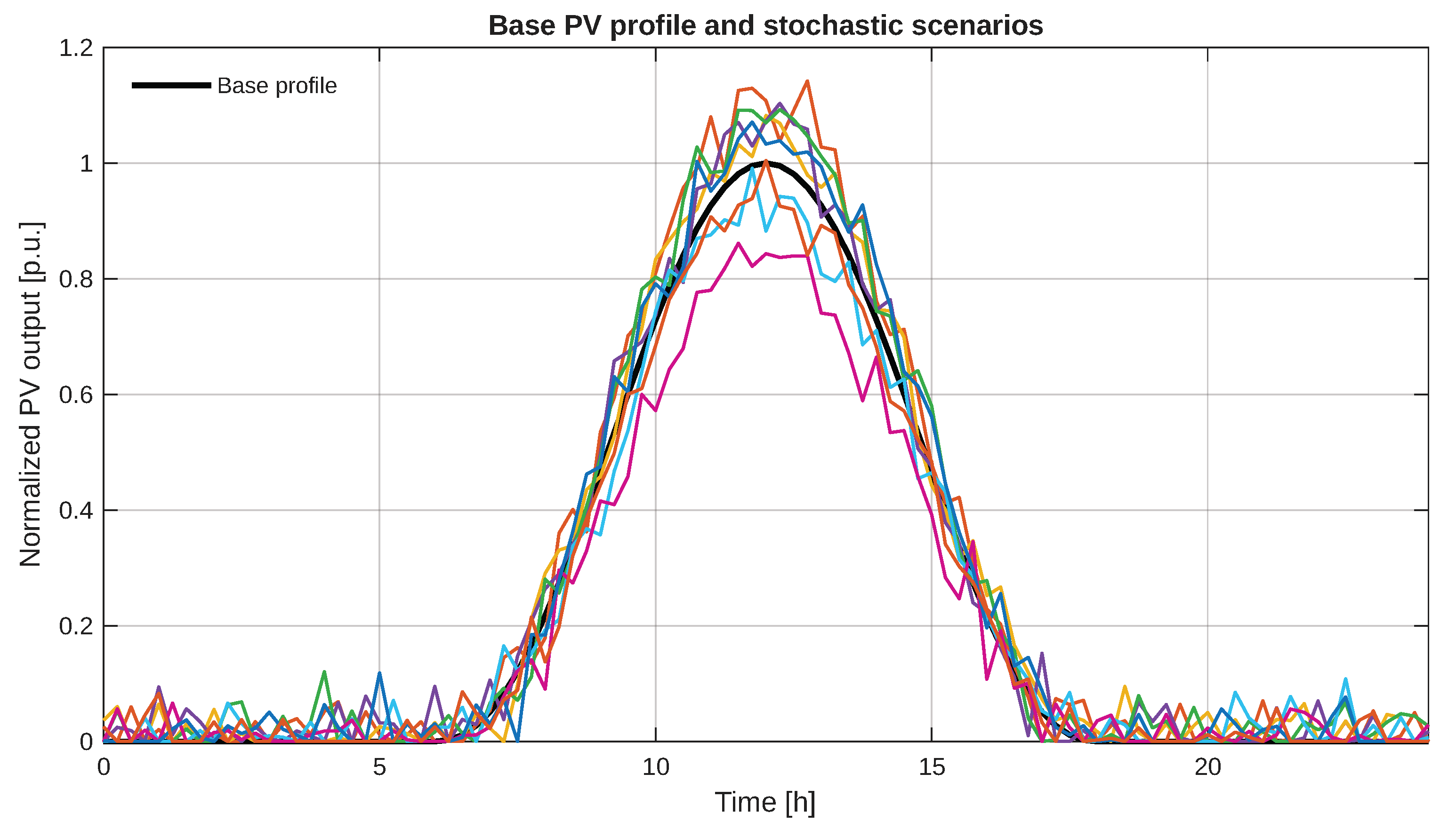
For completeness, Figure 14 depicts the deterministic PV curve and representative stochastic scenarios (used across all experiments). The spread around midday and the attenuation at shoulder hours explain part of the non-monotonic behavior seen in Figure 8: as PV increases, the marginal benefit diminishes when generation occurs away from the highest-risk periods for failures and when reverse flows affect protection coordination.

3.8. Synthesis and Practical Implications

The results convey four consistent messages:

(i)

Climate dominates tail risk. Even with favorable PV support, storms shift distributions and thicken upper tails (Figure 4 and Figure 5), increasing the likelihood of high-impact years.

(ii)

PV provides measurable but saturating reliability gains. Under normal weather, indices improve up to intermediate $r_{\mathrm{PV}}$ (Figure 8); very high PV partially erodes gains due to intermittency, reverse flows and voltage/protection constraints.

(iii)

Compound risk is nonlinear. The $ENS$ surface (Figure 9) shows that for larger $P_{\mathrm{ext}}$ the marginal reliability benefit of PV decreases; resilience investments targeting weather exposure become comparatively more valuable.

(iv)

Rate escalation and base reliability drive outcomes. Sensitivity (Figure 13) ranks $k_{\mathrm{storm}}$ and ${\lambda }_0$ as the most influential levers, informing the prioritization of hardening and maintenance strategies.

From a planning perspective, these findings support a dual-track strategy: (a) mitigate exposure (vegetation management, structure reinforcement, selective undergrounding, sectionalizing and faster fault location/repair) to curb $k_{\mathrm{storm}}$ and effective $P_{\mathrm{ext}}$; and (b) enable DER-friendly operation (adaptive protection, feeder reconfiguration, Volt/VAR and storage) to capture the reliability gains of PV without triggering operational penalties at high penetrations. The framework is sufficiently general to incorporate additional DERs, storage dispatch rules, or correlated weather fields at higher spatial resolution.

4. Discussion

4.1. Interpreting Baseline Behavior

Under normal weather and moderate PV penetration, the distributions of $ENS$, $SAIFI$ and $SAIDI$ are moderately skewed with compact IQRs. The positive dependence among the three indices—especially the near-linear relation of $ENS$ and $SAIDI$—is consistent with classical reliability theory for radial systems [2,5,7]. Dispersion arises from (i) the random alignment of event timing with net-load peaks, (ii) the variability of affected-customer fractions, and (iii) lognormal restoration times, a well-documented feature in distribution operations.

4.2. Weather Dominates Tail Risk

The weather-only experiments show rightward shifts in all index distributions and thicker upper tails, as confirmed by exceedance curves. This agrees with resilience analyses that emphasize correlated, multi-fault states, access constraints and prolonged repairs [3,4]. In our Monte Carlo setting, escalation acts both on the expected number of events (Poisson mean) and on the spread of per-event severities—two multiplicative channels that explain the disproportionate rise in tail metrics (VaR/CVaR). The prioritization emerging from the tornado ranking—reduce base rates ${\lambda }_0$, storm escalation $k_{\mathrm{storm}}$ and storm exposure $P_{\mathrm{ext}}$—is directly aligned with the hardening and interdependency planning literature [12,21].

4.3. Non-Monotonic Reliability Response to PV

In line with [10,14], PV penetration improves reliability up to a practical hosting band, beyond which intermittency, reverse power flow episodes and voltage/protection margins erode the gains. The surface over $(r_{\mathrm{PV}},P_{\mathrm{ext}})$ clarifies that the marginal benefit of PV decreases as storm probability increases; in other words, when the climate term dominates the risk budget, additional PV is not a substitute for hardening and operational resilience.

4.4. Methodological Robustness

Two features improve the credibility of the numerical findings. First, distributional characterization goes beyond mean values: KDEs [17] and exceedance functions quantify shape and tail behavior, which is essential for planning under uncertainty. Second, convergence diagnostics confirm that the adopted number of scenarios ($N=1000$) is sufficient to stabilize sample means [15]. Together, these ensure that reported differences across scenarios are statistically meaningful for the chosen precision.

4.5. Operational Implications

The results suggest a dual-track strategy for utilities:

• Mitigate exposure and escalation: asset hardening and vegetation management to reduce ${\lambda }_0$; reinforcement/undergrounding of critical spans to damp $k_{\mathrm{storm}}$; sectionalizing and automation to reduce correlated impacts (smaller f and faster repairs) [4,12,13].
• Enable DER-friendly operation: adaptive protection, Volt/VAR optimization and (where applicable) storage and microgrid islanding to secure reliability gains at intermediate PV levels [10,20].
• Co-design planning: use the $(r_{\mathrm{PV}},P_{\mathrm{ext}})$ surface as a risk map to coordinate DER hosting with resilience investments, consistent with the broader energy transition [1,11].

4.6. Comparison with Existing Literature: Agreements and Deviations

The obtained trends are broadly consistent with prior reliability and resilience studies, while also providing additional nuances enabled by the unified stochastic–weather pipeline. First, the pronounced rightward displacement and tail thickening of $ENS$, $SAIFI$, and $SAIDI$ under storms agree with the resilience view that extreme weather produces multi-fault states, access limitations, and prolonged restorations [3,4,11]. In our framework, this behavior arises from two coupled mechanisms: an increased expected number of failures (Poisson mean scaled by ${\lambda }_{\mathrm{eff}}$) and a broader per-event severity distribution (larger and more dispersed $f_e$ and $T_{\mathrm{rep},e}$). The resulting amplification of exceedance probabilities is aligned with the “low-probability/high-impact” characterization emphasized in [4,12,21].

Second, the non-monotonic reliability response to PV penetration is in agreement with studies reporting that DERs improve reliability up to a practical hosting band but may saturate or partially erode benefits at very high penetration levels [10,14,20]. Our results add a distributional interpretation to this effect: moderate PV shifts the reliability distributions leftward (lower medians and narrower IQRs), whereas very high PV reduces the separation from the baseline, reflecting increased net-load volatility and the diminishing coincidence between PV generation and high-risk interruption periods. Unlike approaches that only report mean indices, the KDE and exceedance views reveal that PV primarily mitigates central tendency and moderate quantiles, while extreme-weather regimes dominate upper tails regardless of PV level.

Third, the compound-risk surface over $(r_{\mathrm{PV}},P_{\mathrm{ext}})$ provides a quantitative counterpart to the qualitative arguments in resilience planning literature: as storm exposure grows, weather-driven escalation dominates the risk budget and reduces the marginal reliability value of additional PV [4,11,12,21]. The “valley–ridge” structure observed in the ENS heatmap highlights that DER hosting and hardening are complementary rather than substitutable levers, a point that is often mentioned but rarely visualized probabilistically in feeder-level studies.

4.7. Additional Engineering Insights from Distributional Results

Beyond confirming known trends, the distributional results provide several additional insights. (i) The joint scatter and positive dependence among indices indicate that interruption frequency and duration co-vary but are not redundant; some years exhibit moderate $SAIFI$ with high $SAIDI$, producing heavy ENS outcomes. This reinforces the need to evaluate the triplet $(ENS,SAIFI,SAIDI)$ simultaneously rather than relying on a single metric [5,7]. (ii) Tail behaviour is particularly sensitive to weather escalation: even when mean improvements due to PV are visible, storm regimes substantially increase the probability of high-impact years. This suggests that planning based solely on expected indices may underestimate resilience benefits from hardening, especially when utilities face risk constraints or regulatory penalties associated with high-end SAIDI/ENS exceedances. (iii) The convergence diagnostics show that the reported differences across PV and weather regimes are not numerical artifacts but statistically stable comparisons under the adopted scenario budget [15].

From a methodological viewpoint, these insights demonstrate the value of embedding tail-risk diagnostics and robustness checks directly into the reliability pipeline: they enable utilities to interpret not only “how much reliability improves on average” but also “how the worst years change,” which is essential for resilience-oriented decision making.

4.8. Planning Implications under High DER and Climate Exposure

The combined findings support a layered reliability–resilience strategy. On the one hand, asset hardening and exposure mitigation remain the most influential levers, as reflected by the dominance of ${\lambda }_0$, $k_{\mathrm{storm}}$, and $P_{\mathrm{ext}}$ in the tornado ranking. This aligns with long-term resilience investment recommendations emphasizing vegetation management, structural reinforcement, automation, and selective undergrounding [4,12,21]. On the other hand, DER integration provides meaningful reliability gains at intermediate penetration, but these gains persist at higher levels only if supported by DER-friendly operation (adaptive protection, Volt/VAR management, and coordinated switching) [10,14,20].

Practically, the ENS heatmap can be interpreted as a risk map for co-design: when $P_{\mathrm{ext}}$ is low or moderate, PV hosting delivers measurable reliability benefits; when $P_{\mathrm{ext}}$ is high, hardening and rapid restoration logistics yield larger marginal gains. Therefore, utilities should prioritize resilience investments that reduce rate escalation and correlated impacts in parallel with policies that expand DER hosting within a safe operational band.

4.9. Limitations and Extensions

The proposed framework deliberately adopts (i) scenario-level weather flags and (ii) feeder-level aggregation of customer impact. These abstractions are suitable for annual reliability estimation when detailed storm-track, spatial intensity, or asset-level exposure data are unavailable; however, they introduce two main limitations. First, feeder-level aggregation masks the heterogeneity of user-level reliability: localized clusters of vulnerable laterals or critical customers may experience higher $SAIFI/SAIDI$ than the feeder mean, and aggregation can therefore smooth extremes and under-represent inequality in outage exposure. A natural extension is to disaggregate scenarios to the segment or customer-class level, enabling user-weighted indices and spatial risk maps that better capture tail behavior under extreme events.

Second, the protection and switching logic is represented through effective failure/restoration parameters rather than explicit device-level operation. This simplification avoids over-parameterization, but it may shift the estimated interruption frequency and duration if coordination details (e.g., fuse–recloser interaction, adaptive settings, or reverse-power effects under high PV) materially alter fault isolation and restoration times. In practice, this can lead to non-negligible deviations in $SAIFI$-type (frequency-dominated) and $SAIDI$-type (duration-dominated) metrics, especially in feeders with complex sectionalizing layouts or high DER-induced bidirectional flows.

Future work will therefore incorporate: (i) spatially explicit storm fields and crew logistics; (ii) explicit topology reconfiguration under switching and thermal limits [16]; (iii) device-level protection and operational constraints (adaptive protection settings, reverse-flow limits, and voltage margins) to enable comparative studies across alternative feeder configurations; (iv) interdependent communications [21]; and (v) demand response as an adaptive resource under stress [11]. These additions will allow a more detailed identification of how spatial exposure, topology, and protection coordination modulate the saturation or degradation of PV reliability benefits at high penetrations.

5. Conclusions

This work introduced a weather-aware probabilistic framework to quantify feeder-level reliability under high PV penetration. Across the modified IEEE 33-bus case with stochastic load/PV synthesis, weather-dependent failure/restoration, and Monte Carlo estimation of IEEE 1366 indices, the main conclusions are as follows:

C1. Extreme weather sets the risk budget. Under storm conditions, the empirical distributions of ENS, SAIFI and SAIDI shift to higher values and widen, revealing heavier upper tails. Planning should therefore consider tail metrics and exceedance behavior, not means alone.

C2. PV delivers measurable but saturating gains. Under normal weather, increasing PV from zero to moderate levels (around 30–35%) consistently lowers ENS, SAIFI and SAIDI. Beyond that band, benefits flatten or slightly erode due to intermittency, reverse-flow episodes and operational constraints.

C3. Compound risk is nonlinear and context-dependent. The ENS response surface over PV penetration and storm probability exhibits a valley at moderate PV and a ridge as storm likelihood increases. As climate exposure grows, the marginal reliability benefit of additional PV diminishes; DER hosting must be co-optimized with resilience measures.

C4. Dominant drivers are failure-rate escalation and exposure. Sensitivity analysis ranks the base failure rate and the storm escalation factor as the most influential contributors to ENS, followed by storm probability and mean repair/restoration effects. Targeted actions (hardening, vegetation/weatherproofing, selective undergrounding, sectionalizing and faster restoration logistics) yield the largest risk reductions.

C5. Resilience under long events shows a characteristic drop–plateau–recovery. The 72 h stress test exhibits an initial shock, a stressed plateau with served fraction well below nominal, and a multi-hour recovery, providing an interpretable scalar resilience measure from the area under the curve.

C6. Methodological robustness and auditability. Kernel densities, exceedance curves, boxplots and convergence diagnostics show that the adopted scenario budget is sufficient and that the reported differences across scenarios are statistically stable for the precision targets used here.

Practical implication. For feeders similar to the studied case, the best reliability–resilience trade-off arises from combining moderate PV penetration with exposure mitigation (reducing ${\lambda }_0$ and storm escalation) and enabling DER-friendly operation (adaptive protection, Volt/VAR control and reconfiguration) so that PV gains persist at higher penetrations.

Future work. Extensions include spatial storm fields and crew logistics, explicit device-level protection and switching constraints, storage and microgrid islanding, and interdependency with communications.

References

- International Energy Agency. Renewables 2022: Analysis and Forecast to 2027; IEA: Paris, France, 2022. Available online: https://www.iea.org/reports/renewables-2022 (accessed on 15 November 2024).
- Brown, R.E. Electric Power Distribution Reliability, 2nd ed.; CRC Press: Boca Raton, FL, USA, 2009. [Google Scholar]
- Panteli, M.; Mancarella, P. Influence of extreme weather and climate change on the resilience of power systems: Impacts and possible mitigation strategies. Electr. Power Syst. Res. 2015, 127, 259–270. [Google Scholar] [CrossRef]
- Panteli, M.; Mancarella, P. Modeling and evaluating the resilience of critical electrical power infrastructure to extreme weather events. IEEE Syst. J. 2017, 11, 1733–1742. [Google Scholar] [CrossRef]
- Billinton, R.; Allan, R.N. Reliability Evaluation of Power Systems, 2nd ed.; Springer: Berlin/Heidelberg, Germany, 1996. [Google Scholar]
- Billinton, R.; Allan, R.N. Reliability Evaluation of Power Systems; Springer: New York, NY, USA, 1994. [Google Scholar]
- IEEE Std 1366-2022; IEEE Guide for Electric Power Distribution Reliability Indices. Technical Report. IEEE: New York, NY, USA, 2022. [CrossRef]
- Karki, R.; Billinton, R. Reliability/cost implications of PV and wind energy utilization in small isolated power systems. IEEE Trans. Energy Convers. 2001, 16, 368–373. [Google Scholar] [CrossRef]
- Billinton, R.; Wangdee, T. Reliability-based transmission reinforcement planning associated with large-scale wind farms. IEEE Trans. Power Syst. 2007, 22, 34–41. [Google Scholar] [CrossRef]
- Aschidamini, G.L.; da Cruz, G.A.; Resener, M.; Leborgne, R.C.; Pereira, L.A. A framework for reliability assessment in expansion planning of power distribution systems. Energies 2022, 15, 5073. [Google Scholar] [CrossRef]
- Nogal, M.; O’Connor, A.; Martinez-Pastor, B.; Caulfield, B. Novel probabilistic resilience assessment framework of transportation networks against extreme weather events. ASCE-ASME J. Risk Uncertain. Eng. Syst. Part A Civ. Eng. 2017, 3, 3. [Google Scholar] [CrossRef]
- Ryu, H.; Chae, W.; Kim, H.; Cho, J. Mid- to long-term distribution system planning using investment-based modeling. Energies 2025, 18, 3702. [Google Scholar] [CrossRef]
- Ngoko, B.O.; Sugihara, H.; Funaki, T. Synthetic generation of high temporal resolution solar radiation data using Markov models. Sol. Energy 2014, 103, 160–170. [Google Scholar] [CrossRef]
- Adegoke, S.A.; Sun, Y.; Adegoke, A.S.; Ojeniyi, D. Optimal placement of distributed generation to minimize power loss and improve voltage stability. Heliyon 2024, 10, e39298. [Google Scholar] [CrossRef] [PubMed]
- Lin, W.; Su, C. An efficient Monte-Carlo simulation for the dynamic reliability analysis of jacket platforms subjected to random wave loads. J. Mar. Sci. Eng. 2021, 9, 380. [Google Scholar] [CrossRef]
- Baran, M.E.; Wu, F.F. Network Reconfiguration in Distribution Systems for Loss Reduction and Load Balancing. IEEE Trans. Power Deliv. 1989, 4, 1401–1407. [Google Scholar] [CrossRef]
- Silverman, B.W. Density Estimation for Statistics and Data Analysis; Chapman and Hall: London, UK, 1986. [Google Scholar]
- Téllez, A.A.; Ortiz, L.; Ruiz, M.; Narayanan, K.; Varela, S. Optimal Location of Reclosers in Electrical Distribution Systems Considering Multicriteria Decision Through the Generation of Scenarios Using the Montecarlo Method. IEEE Access 2023, 11, 68853–68871. [Google Scholar] [CrossRef]
- Peña, D.; Aguila Téllez, A.; Jurado, F. Reliability Assessment of Ecuador’s Power System: Metrics, Vulnerabilities, and Strategic Perspectives. Energies 2025, 18, 3059. [Google Scholar] [CrossRef]
- Wang, J.; Chang, X.; Feng, L.; Zhao, J. Reliability Evaluation of Distribution Network Considering Uncertainty of Photovoltaic Generation Output. In Proceedings of the 2020 5th Asia Conference on Power and Electrical Engineering (ACPEE), Chengdu, China, 4–7 June 2020. [Google Scholar] [CrossRef]
- Home-Ortiz, J.M.; Yamaguti, L.C.; Yumbla, J.; Melgar-Dominguez, O.D.; Monaro, R.M.; Mantovani, J.R. Resilience-oriented planning for distribution systems combining distributed generation allocation and dynamic operational strategies. IEEE Access 2025, 13, 154556–154567. [Google Scholar] [CrossRef]
Figure 2.
Baseline reliability performance (normal weather, ). Boxplots for , and computed from Monte Carlo scenarios.
Figure 3.
Pairwise correlation between , and under baseline conditions. The positive association highlights the joint movement of frequency, duration and energy not supplied.
Figure 4.
Empirical probability densities of , and under normal vs. storm regimes. Storms shift and spread the distributions due to escalated failure rates and heavier restoration dispersion.
Figure 5.
Exceedance probability of for normal vs. storm regimes. The rightward displacement of the storm curve reveals a substantially heavier upper tail.
Figure 6.
Normal vs. storm: distributional comparison of , and . Storms degrade both central tendency and dispersion across all indices.
Figure 7.
Resilience stress-test over 72 h: disturbance-recovery trajectory (served fraction). The shaded shape captures initial shock, stressed plateau and recovery slope, illustrating compound restoration dynamics.
Figure 8.
Reliability indices versus PV penetration under normal weather. Each subplot reports the sample mean and 95% CI for (top) [kWh], (middle) [int/customer·yr], and (bottom) [h/customer·yr]. The curves show improvement up to intermediate PV levels and saturation/slight degradation at very high .
Figure 9.
heatmap as a function of PV penetration and storm probability . PV gains are visible at low-to-moderate , while higher storm likelihood dominates the response.
Figure 10.
Summary across scenario families (Normal, Storm, PV15, PV35, PV60). Moderate PV improves all indices; storms worsen level and spread; very high PV partially erodes the gains.
Figure 11.
Correlation of indices (
,
) with the ordered scenario index across families. Signs and magnitudes are consistent with the improvements/degradations seen in
Figure 12.
Convergence of sample means for , and with the number of scenarios k. The stabilization before supports the chosen Monte Carlo budget.
Figure 13.
OAT tornado sensitivity on mean reliability indices (, and ). Failure-rate parameters (, ) and storm exposure () dominate across metrics, while restoration parameters mainly modulate duration- and energy-based outcomes.
Figure 14.
Deterministic PV curve and representative stochastic realizations (diagnostic).