Article

Trend Prediction of Valve Internal Leakage in Thermal Power Plants Based on Improved ARIMA-GARCH

1
Shanxi Century Central Test Electricity Science &Technology Co., Ltd., Taiyuan 030032, China
2
School of Energy, Power and Mechanical Engineering, North China Electric Power University, Beijing 102206, China
*
Author to whom correspondence should be addressed.
Energies 2025, 18(23), 6275; https://doi.org/10.3390/en18236275 (registering DOI)
Submission received: 23 October 2025 / Revised: 21 November 2025 / Accepted: 26 November 2025 / Published: 28 November 2025

Abstract

Accurate trend prediction of valve internal leakage is crucial for the safe and economical operation of thermal power units. To address the issues of prediction lag and insufficient accuracy in existing methods when dealing with the dynamic changes in internal leakage, this paper proposed an Improved Autoregressive Integrated Moving Average–Generalized Autoregressive Conditional Heteroskedasticity (IARIMA-GARCH) method that integrated Multi-Time-Scale Decomposition, an Improved ARIMA (IARIMA) model, and an Improved GARCH (IGARCH) model for accurate prediction of drain valve internal leakage. First, using a Multi-Time-Scale Decomposition method based on sampling at different time intervals, the original valve internal leakage time series were reconstructed into three characteristic subsequences—short-term, medium-term, and long-term—to capture the evolutionary features at various time scales. Then, an IARIMA model, employing the Huber loss function for robust parameter estimation, was constructed as the leakage prediction model to effectively suppress the interference of outliers. Simultaneously, an IGARCH model was built as the leakage volatility prediction model by introducing the previous moment’s volatility to correct the current residual, establishing a feedback mechanism between the mean and volatility equations, thereby enhancing the characterization of volatility clustering. Finally, using a weight coefficient dynamic calculation method based on RMSE, the Multi-Time-Scale prediction results of each subsequence were fused to obtain the final predicted valve internal leakage. Taking the main steam drain valve of a thermal power plant as the research object, and using Mean Absolute Error (MAE), Root-Mean-Squared Error (RMSE), Mean Absolute Percentage Error (MAPE), and symmetric Mean Absolute Percentage Error (sMAPE) as evaluation metrics, a case study on trend prediction of drain valve internal leakage was conducted, comparing the proposed method with ARIMA, Long Short-Term Memory networks (LSTM) and eXtreme Gradient Boosting (XGBoost) methods. The results showed that compared to ARIMA, LSTM and XGBoost, the proposed IARIMA-GARCH method achieved the lowest values on error metrics such as Mean Absolute Error (MAE), Root-Mean-Squared Error (RMSE), Mean Absolute Percentage Error (MAPE), and symmetric Mean Absolute Percentage Error (sMAPE), and its Coefficient of Determination (R2) is closest to 1. The standardized residual sequence most closely resembled a white noise sequence with zero mean and unit variance, and its distribution was the closest to a normal distribution. This proved that the IARIMA-GARCH method possessed higher prediction accuracy, stronger dynamic adaptability, and superior statistical robustness, providing an effective solution for valve condition prediction and predictive maintenance.

1. Introduction

As key components in the thermal system of power units, the tightness of drain valves directly affects the thermal economy and operational safety of the unit. Constructing high-precision internal leakage prediction models is essential for effectively assessing the health status of drain valves and anticipating their performance degradation trends [1]. The accurate extraction of dynamic trends and degradation features from valve internal leakage time series directly determines how well future leakage increases can be predicted and how accurately the remaining useful life can be estimated. This predictive capability, in turn, critically impacts the formulation of proactive maintenance strategies and the prevention of unplanned shutdowns [2].
In the field of industrial equipment condition prediction, research methods can be primarily divided into two categories: physics-based models and data-driven methods. The former, such as modeling based on fluid dynamics [3] and structural mechanics [4], requires precise knowledge of the internal structure and degradation mechanisms of the equipment. While physically interpretable, it is often difficult to build accurate analytical models for complex internal faults like valve internal leakage, limiting their practicality. In contrast, data-driven methods directly mine patterns from historical operational data, avoiding complex physical mechanism modeling, and have become the mainstream approach in current research [5]. These methods can be further divided into traditional statistical learning models, machine learning methods, and deep learning models. Traditional statistical learning models, such as the Autoregressive Moving Average (ARMA), offer notable advantages including concise model structures and strong parameter interpretability, demonstrating robust performance in stationary time series forecasting. However, the development process of valve internal leakage often involves nonlinear and non-stationary characteristics induced by operational fluctuations, which are challenging for conventional linear statistical models to capture effectively, leading to a significant decline in prediction accuracy. Classical machine learning models, such as Support Vector Machines (SVM) [6] and Random Forests [7], exhibit good generalization performance under small-sample conditions in the case of the former, yet their predictive effectiveness heavily relies on the quality of feature engineering—an aspect often constrained by sensor configuration and measurement noise in valve leakage scenarios. The latter, while capable of effectively assessing feature importance and providing variable contribution rankings, operates under an inherent assumption of sample independence, thereby overlooking temporal dependencies within the data and potentially missing dynamic correlation information crucial for state evolution analysis. Models specifically designed for time series, such as Facebook’s open-source Prophet [8], incorporate built-in components for trend, seasonality, and holiday effects, enabling fast fitting; however, they lack flexibility in handling complex patterns commonly encountered in valve operations, such as non-Gaussian noise and heteroscedastic fluctuations, making them less adaptable to the specificities of industrial field data. Modern deep learning models, such as Recurrent Neural Networks (RNN) [9], Convolutional Neural Networks (CNN) [10], Long Short-Term Memory networks (LSTM), and the recently emerging Transformer architecture [11], demonstrate significant advantages in complex time series forecasting tasks due to their powerful sequence modeling capabilities and ability to capture long-term dependencies. However, their high model complexity, training costs, and substantial data requirements, coupled with inherent limitations like imbalance between exploration and exploitation, poor convergence, and susceptibility to local optima, constrain their application effectiveness in this field. When existing methods are applied to valve internal leakage trend prediction, a prevalent prediction lag phenomenon is observed. Specifically: predictions based on traditional statistical methods typically exhibit a systematic lag of 3–5 sampling periods, with lag errors showing a right-skewed distribution, resulting in severe underestimation of actual leakage during sudden increases. While deep learning models can capture complex nonlinear relationships, they still demonstrate transient lags of 2–3 periods during operational condition mutations, displaying distinct peak- and-thick-tailed characteristics. This prediction lag not only delays fault warning timing but also leads to maintenance decision biases, directly affecting unit operational safety and economic performance.
The ARMA model [12] and Generalized Autoregressive Conditional Heteroskedasticity (GARCH) model [13], as classical time series analysis tools, hold an important position in the prediction and modeling of equipment degradation processes. ARMA model is adept at capturing short-term autocorrelation and stationary fluctuations in time series. Ref. [14] employed the VMD-ARMA-SSMUSIC method to perform modal decomposition, denoising, and residual prediction on leak acoustic emission signals from high-temperature, high-pressure steam superheater pipes. This approach significantly improved single-point leak localization accuracy, providing an effective means for pipeline safety monitoring in extreme thermal environments. The GARCH model focuses on characterizing the “clustering” feature of time series volatility. Ref. [15] applied the GARCH-MIDAS framework to model investor sentiment and economic policy uncertainty at mixed frequencies. This approach significantly improved the out-of-sample prediction accuracy of international daily return volatility. The enhanced forecasts provide a solid basis for real estate trust investment decisions in uncertain environments. However, when directly applying ARMA or GARCH to valve internal leakage prediction, their inherent drawbacks become apparent: Firstly, they are essentially linear models and struggle to effectively capture the potentially complex nonlinear dynamic characteristics in the evolution of internal leakage [16]. Secondly, they require strict stationarity of the time series, whereas actual equipment degradation processes are typically non-stationary, necessitating complex preprocessing like differencing, which may lead to the loss of some trend information. Thirdly, standard ARMA/GARCH models typically assume the disturbance term follows a normal distribution during parameter identification [17,18], while noise in real industrial data often violates this assumption, affecting model accuracy.
To overcome the limitations of the aforementioned methods, researchers have proposed various improvement strategies, mainly focusing on two directions. One direction involves enhancing the prediction performance of a single algorithm [19,20,21]. A representative example is the DRIFT system [19], which integrates LSTM with deep reinforcement learning for dynamic crowd inflow control. This approach significantly improves throughput and management efficiency in public spaces through intelligent decision-making, offering an innovative solution for complex crowd management scenarios. The more important improvement direction is to adopt hybrid optimization methods, combining the advantages of different algorithms to enhance prediction accuracy [22,23,24,25]. For example: Ref. [23] addressed the optimization problem of solar maximum power point tracking (MPPT) by proposing a hybrid algorithm combining the salp swarm algorithm (SSA) with the perturb and observe (P&O) method. The approach enhanced SSA through the incorporation of a dynamic spiral evolution mechanism and Lévy flight strategy, employed Gaussian operators for distributed computation, and achieved fine-grained search with small step sizes through integration with the P&O method. This ensures rapid convergence and further suppresses power oscillations after convergence. The method effectively resolves issues of low convergence and poor tracking accuracy in MPPT optimization. Ref. [24] proposed a hybrid approach using feedforward MLP and LSTM networks to improve fault diagnosis and remaining useful life (RUL) prediction for rolling bearings. The model leverages the strengths of both architectures: MLP captures complex nonlinear relationships while LSTM handles sequential dependencies. This approach can significantly reduce unplanned downtime and extend the service life of critical machinery.
In summary, the innovations of this paper lie in the following: (1) Proposing a Multi-Time-Scale Decomposition fusion mechanism. The original leakage time series is decomposed into short-term, medium-term, and long-term subsequences. A dynamic weighting strategy, informed by the recent predictive performance of each sub-model, is then applied to fuse these multi-scale forecasts. This mechanism effectively overcomes the lag inherent in fixed prediction windows when confronting abrupt condition changes, thereby enhancing the model’s dynamic adaptability. (2) Constructing a deeply coupled Improved ARIMA-GARCH (IARIMA-GARCH) combined prediction model. This model is improved at two levels: firstly, introducing the Huber loss function into the ARIMA model for robust parameter estimation to suppress outlier interference and enhance model robustness; secondly, innovatively introducing the previous moment’s volatility as feedback into the GARCH model to correct the current residual, establishing a dynamic link between the mean and variance equations, thereby more accurately characterizing the volatility clustering features of the internal leakage sequence. Taking the main steam drain valve of a thermal power plant as the research object, a case study on valve internal leakage prediction was conducted for validation. Using Mean Absolute Error (MAE), Root-Mean-Squared Error (RMSE), Mean Absolute Percentage Error (MAPE), symmetric Mean Absolute Percentage Error (sMAPE), and Coefficient of Determination (R2) as performance metrics, IARIMA-GARCH analysis results were compared with ARIMA, LSTM and eXtreme Gradient Boosting (XGBoost) methods, proving that IARIMA-GARCH outperforms the other three methods in both prediction accuracy and dynamic adaptability, providing an effective technical approach for accurate valve condition prediction and predictive maintenance.

2. The Overall Idea of the IARIMA-GARCH Prediction Model

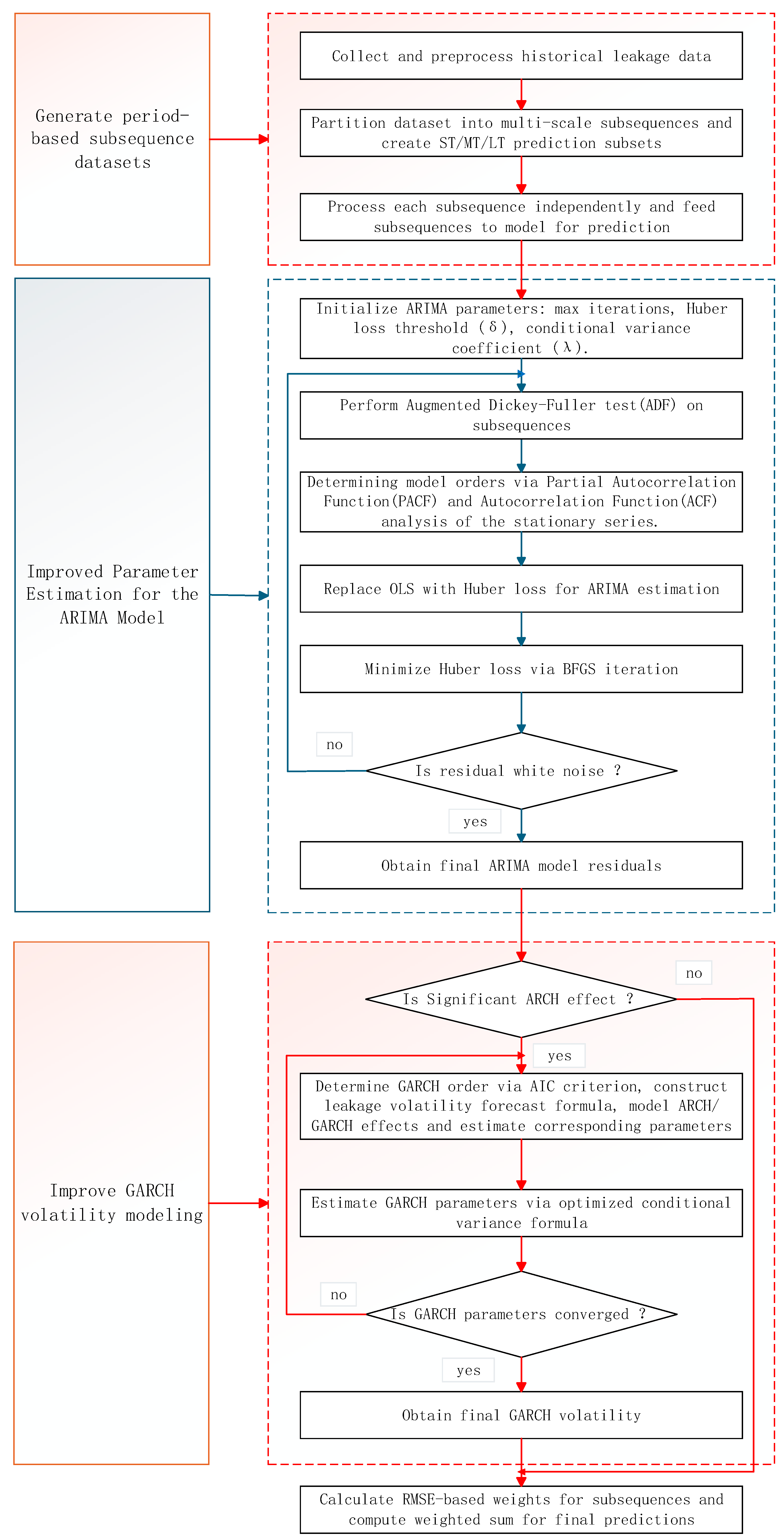
This paper proposed an IARIMA-GARCH method for predicting the valve internal leakage in thermal power plants. The overall framework of the IARIMA-GARCH method was shown in Figure 1.
The specific steps of the IARIMA-GARCH method were as follows:
(1)
Collect historical operational data of univariate valve internal leakage, which consists of time-sequenced measurements of internal valve leakage. Preprocess the historical internal leakage data, and construct the drain valve internal leakage prediction dataset.
(2)
Before inputting the dataset into the prediction model, initialize model parameters, including the maximum number of iterations, the Huber loss threshold δ, and the conditional variance coefficient λ in the residual term.
(3)
Utilize the IARIMA-GARCH method to achieve valve internal leakage prediction for thermal power plants.
(1)
Decompose the valve internal leakage time series into short-term, medium-term, and long-term subsequences according to different prediction periods using the Multi-Time-Scale Decomposition method to capture evolutionary characteristics at different time scales.
(2)
Use the Huber loss function instead of the OLS function to construct the IARIMA model as the internal leakage prediction model, optimizing the key parameters of the ARIMA model to effectively suppress the interference of outliers.
(3)
By introducing the previous moment’s volatility to correct the current residual, construct the Improved GARCH (IGARCH) model as the internal leakage volatility prediction model, establishing a feedback mechanism between the mean and volatility equations to enhance the characterization of volatility clustering.
(4)
Dynamically calculate weights based on the prediction errors of each subsequence, and fuse the multi-scale prediction results to obtain the optimized internal leakage prediction value.
(4)
Obtain the final internal leakage prediction value and conduct a comparative study with the test dataset to evaluate prediction accuracy and error analysis.

3. Implementation of IARIMA-GARCH Method

As shown in Figure 2, to implement the IARIMA-GARCH method, it is crucial to sequentially address the construction of the multi-scale prediction framework, the IARIMA model, and the IGARCH model.

3.1. Construction of the Multi-Time-Scale Prediction Framework

To overcome the limitations of a single model in characterizing the multi-scale features of time series, this paper proposes a Multi-Time-Scale Decomposition method to establish a multi-scale prediction framework [25]. This is done by constructing short-term, medium-term, and long-term subsequence datasets to address the heterogeneity at different time dimensions in the original series and avoid estimation bias caused by pattern coupling. The specific steps are as follows:
(1)
Based on the internal leakage prediction dataset Q L , directly truncate a segment of length TD from the internal leakage data to form the short-term subsequence dataset Q D , expressed as:
Q D = Q D L , 1 , Q D L , 2 , , Q D L , i , , Q D L , T D T D
where TD is the subsequence length
(2)
Based on the internal leakage prediction dataset Q L , take the average of every N k internal leakage values to obtain Q D Z , i , forming the medium-term scale subsequence dataset Q Z , as follows:
Q Z = Q D Z , 1 , Q D Z , 2 , , Q D Z , i , , Q D Z , T Z T Z
Q D Z , i = 1 N k j   =   ( i     1 ) N k   +   1 i N k Q D L , j
where TZ is the subsequence length.
(2)
Based on the internal leakage prediction dataset   Q L , take the average of every N j internal leakage values (where N j > N k ) to obtain   Q C L , i , forming the long-term scale subsequence dataset Q C L , as follows:
Q C L = Q C L , 1 , Q C L , 2 , , Q C L , T C T C
Q C L , i = 1 N j j   =   ( i     1 ) N j   +   1 i N j Q C L , j
where TC is the subsequence length.

3.2. Improved ARIMA Model

Parameter estimation for the ARIMA model based on the Ordinary Least Squares (OLS) method is highly sensitive to abnormal observations, potentially leading to severe estimation bias. This paper proposes using the Huber loss function instead of OLS for parameter estimation to achieve intelligent optimization of the key parameters of the ARIMA model. The specific steps are as follows:
(1)
Initialize the ARIMA model parameters, including the maximum number of iterations, the Huber loss threshold δ, and the conditional variance coefficient λ in the residual term, among others.
(2)
Data Stationarity Processing and Model Order Determination.
Perform the Augmented Dickey–Fuller (ADF) stationarity test on the subsequence datasets obtained from Multi-Time-Scale Decomposition to determine the differencing order d. Perform differencing for stationarity on each subsequence dataset. The expression is:
z t ( d ) = d Q t = ( 1 B ) d Q t
where z t ( d ) is the stationary series in the ARIMA model; d represents the d-th order differencing operator; d is the differencing order, d ≤ 2; B is the lag operator; and Q t represents the subsequence sets, and is the general term for Q Z ,   Q C L and Q D .
Determine the model order q based on the Autocorrelation Function (ACF) of the stationary series z t ( d ) , as shown below:
ς ^ = 1 T t = 1 T z t
γ ^ 0 = 1 T t = 1 T ( z t ς ) 2
γ ^ k = 1 T t   =   k + 1 T ( z t ς ^ ) ( z t k ς ^ )
ρ ^ k = γ ^ k γ ^ 0
where ρ ^ k represents the autocorrelation function value of the time series at lag order k; γ ^ k represents the autocovariance function of the time series at lag order k; γ ^ 0 represents the variance of the time series; and ς ^ represents the mean of the time series.
Determine the model order p based on the Partial Autocorrelation Function (PACF) of the stationary series z t ( d ) , as shown below:
φ k k = C o r r ( z t , z t k / z t 1 , z t 2 , , z t k + 1 )
z t = φ k 1 z t 1 + φ k 2 z t 2 + + φ k k z t k + ω t
where φ k k represents the partial autocorrelation coefficient at lag order k; ω t represents the error term, assumed to be a white noise sequence; z t 1 , z t 2 , , z t k represent the lagged observations; and φ k 1 , φ k 2 , φ k k 1 represent the regression coefficients.
The aforementioned Equations (7)–(12) define the estimation algorithms for ACF and PACF of a stationary time series, providing the theoretical foundation for the preliminary identification of model orders. However, the determination of parameters p and q is not derived from a direct solution of these formulas but rather constitutes a model identification process based on statistical inference. Specifically, if the PACF plot exhibits a cut-off after lag p, indicating that the partial autocorrelation coefficients approach zero and show no significant correlation beyond this point, the autoregressive (AR) order is determined to be p. Conversely, if the ACF plot shows a cut-off after lag q, the moving average (MA) order is identified as q.
(3)
Improved ARIMA Model Parameter Estimation
After obtaining the model orders from the PACF and ACF plots, substitute the values into the initial model and calculate the series prediction value as:
z t ^ = μ + i   =   1 p ϕ i z t i + j   =   1 q θ j e t j
where z t ^ is the predicted value of the stationary series at time t; μ is the model constant term, it is learned from the observed data through the model fitting process; ϕ i is the autoregressive coefficient of the AR part; θ j is the moving average coefficient of the MA part; z t i is the lagged term of the stationary series; and e t j is the prior residual term.
Calculate the residual after obtaining the predicted value z t ^ :
e t = z t z t ^
where e t is the residual at time t.
Compare the calculated residual e t and δ . If e t > δ , it indicates an outlier at this moment. Then use the Huber loss function instead of OLS for parameter estimation. The expression is:
L δ ( e t ) = 1 2 e t 2 e t δ δ ( e t 1 2 δ ) e t > δ
where L δ ( e t ) is the Huber loss value at time t, and δ is the threshold of the Huber loss function, usually δ = 1.345, but can be adjusted according to data characteristics.
The goal of model parameter estimation is to minimize the total Huber loss:
ϕ i = min ϕ i t   =   1 n L δ ( e t )
Since the stationary series z t satisfies:
z t = μ + i   =   1 p ϕ i z t i + j   =   1 q θ j e t j + e t  
Rewrite Formula (17) into linear regression form:
z t = x t Θ + e t
The regression vector and parameter vector are, respectively:
x t = ( 1 , z t 1 , , z t p , e t 1 , , e t q )
Θ = ( μ , ϕ 1 , , ϕ p , θ 1 , , θ q )
Thus, the residual is:
e t = z t x t Θ
From Formula (15), the gradient of the objective function with respect to Θ is:
L ( Θ ) = 1 T t = 1 T ψ δ ( e t ) x t
where the influence function is:
ψ δ ( e i ) = e i e t δ δ s i g n ( e i ) e t > δ
Denote the parameters at step k as Θ k , the inverse Hessian approximation as H k (initial H 0 = I ), and the search direction as:
d k = H k L ( Θ k )
Obtain the step size α k through strong Wolfe line search, and update:
Θ k + 1 = Θ k + α k d k
Let:
s k = Θ k + 1 Θ k  
y k = L ( Θ k + 1 ) L ( Θ k )
Then the inverse Hessian is updated by BFGS correction:
H k + 1 = ( I s k y k y k s k ) H k ( I y k s k y k s k ) + s k s k y k s k  
Iterate until the gradient norm L ( Θ k ) < ε or the maximum number of iterations k m a x is reached. Finally, obtain the robust estimate:
Θ ^ = Θ k  
where ψ δ ( e i ) represents the influence function (derivative of Huber loss); H k represents the inverse Hessian approximation at step k; s k represents the parameter increment; y k represents the gradient increment; I represents the identity matrix, with the same dimensions as the Hessian (p × p, where p is the number of parameters), with 1 s on the diagonal and 0 s elsewhere, serving only to “maintain dimension invariance”; ε represents the convergence tolerance; and k m a x represents the maximum number of iterations.
(4)
Obtain the predicted value z t ^ from the ARIMA model, and then derive the corresponding internal leakage prediction value Q t ^ .

3.3. Improved GARCH Model

The core idea of the combined prediction is to feed the residuals e t calculated during the ARIMA model prediction process into the GARCH model. This optimizes the residual calculation of the GARCH model itself while combining the two prediction models to forecast future value volatility. Typically, the ARIMA and GARCH models are connected in a simple series mode. This paper introduces the conditional variance from the previous time step into the calculation of the current residual, allowing the residual calculation of the ARIMA model to incorporate “uncertainty information of volatility” in advance.
(1)
GARCH Effect Test
First, perform an ARCH effect test on the residual sequence e t of the mean equation. Construct the squared residual sequence ϵ t = e t 2 , and estimate the auxiliary regression:
ϵ t = α 0 + i   =   1 q α i ϵ t i + u t
Simultaneously calculate the LM statistic:
L M = T R 2
where α 0 is the constant term of the auxiliary regression; α i represents the coefficients of the auxiliary regression, all zero under the null hypothesis; u t is the error term of the auxiliary regression; T is the sample size of the auxiliary regression; and R 2 is the coefficient of determination of the auxiliary regression. Under the null hypothesis H 0 : α 1 = α 2 = = α q = 0 (no ARCH effect), if the p-value of the test statistic is <0.05, reject the null hypothesis, indicating the presence of ARCH effects, making it suitable to build a GARCH model.
(2)
GARCH Model Order Determination
Determine the GARCH model order using the Akaike Information Criterion (AIC). That is, among all candidate order combinations (m, n), select the GARCH(m, n) model that minimizes the AIC value as the optimal order.
After determining the order of the GARCH model, predict the future volatility of the internal leakage:
σ t 2 = ω + i   =   1 m α i e t 2 + j   =   1 n β j σ t j 2
where σ t 2 is the conditional variance at time t, the predicted variance based on all information before time t;   σ t is the predicted volatility value at time t; ω is the constant term (intercept); α i represents the coefficients of the ARCH term, measuring the contribution of past squared errors to the current conditional variance; β j represents the coefficients of the GARCH term, measuring the contribution of past conditional variances to the current conditional variance; and the constraint conditions ω > 0 ,   α i 0 ,   β j 0 ,   α i + β j < 1 must be satisfied to obtain the optimal parameters to be estimated.
Assuming the residuals e t follow a normal distribution, use the Maximum Likelihood Estimation method to estimate the parameters ω , α 1 , α n , β 1 , , β m :
H ( ω , α 1 , α n , β 1 , , β m ) = max ω , α n , β m t = 1 N 1 2 l n ( 2 π ) 1 2 l n ( σ t 2 ) e t 2 2 σ t 2
where H ( ω , α 1 , α n , β 1 , , β m ) represents the log-likelihood function value, and N is the sample size (the total number of observations in the sequence). Construct the log-likelihood function based on the distribution of the disturbance term, and use the BFGS numerical algorithm to solve the maximization of the likelihood function, obtaining the final parameter values.
The stability of the BFGS algorithm stems from its core mechanism: iteratively updating a positive definite inverse Hessian matrix approximation (Hk) to simulate the local curvature information of the objective function. Compared to the classical Newton method, which requires direct computation and inversion of the Hessian matrix—a process that may fail when the parameter space is far from the optimum due to the Hessian matrix not being positive definite—the BFGS algorithm ensures that its inverse Hessian approximation Hk remains positive definite throughout the entire iterative process by employing a rank-two update formula. This characteristic guarantees that the algorithm always generates a search direction that decreases the objective function value, thereby effectively avoiding numerical oscillations or even divergence issues caused by incorrect search directions. This makes BFGS particularly robust when dealing with likelihood functions that have complex curvature structures. Furthermore, under the ideal assumption that the objective function (such as the robust likelihood function adopted in this study) is twice continuously differentiable and uniformly convex, the BFGS algorithm has been proven to achieve a superlinear convergence rate. This means that in the later stages of iteration, its convergence speed is significantly faster than the linear convergence of gradient descent methods, enabling it to approach a local optimum with fewer iteration steps. This ensures the reliability and validity of the model parameter estimation results.
(3)
Improved Residual Term Calculation
Typically, a single serial configuration is adopted between the ARIMA and GARCH models, whereby the conditional variance from the previous time step is incorporated into the calculation of the current residual. This integration allows the residual computation of the ARIMA model to proactively account for the “uncertainty information of volatility.” By introducing the prior period’s conditional variance into the residual calculation Equation (14), the modified residual is obtained:
e t = z t z t ^ λ σ t 1
where λ is the weight coefficient (the conditional variance coefficient).
Substitute the improved residual term back into Formula (32) to obtain the updated conditional variance formula:
σ t 2 = ω + i = 1 m α i e t i 2 + j = 1 n β j σ t j 2
After calculating the volatility, the subsequence internal leakage prediction value is the sum of the mean internal leakage prediction value Q t ^ and the internal leakage volatility, expressed as:
Q L ^ = Q t ^ ± σ t

3.4. Multi-Time-Scale Prediction Result Fusion

Based on the prediction values obtained from the short-term, medium-term, and long-term subsequences with different time spans, use the RMSE weight coefficient calculation evaluation method to fuse the Multi-Time-Scale prediction results and obtain the optimized internal leakage prediction value. Let the weight proportions of the short-term, medium-term, and long-term subsequences be “a”, “b”, “c”, respectively. The weight formula is:
a , b , c = 1 ( E n , t + ε ^ ) n D , Z , C 1 ( E n , t + ε ^ )
E n , t = 1 N n i   =   t n   +   1 t ( z t z t ^ ) 2
where E n , t represents the error metric based on RMSE; N n represents the number of samples in the subsequence; and ε ^ represents an arbitrarily small positive number much smaller than the normal error, preventing division by zero error when “the error happens to be 0”. a, b, c satisfy a > 0 , b > 0 , c > 0 and a + b + c = 1 .
The final prediction result is obtained by multiplying the internal leakage prediction values of the three subsequences by their respective weight ratios and summing them up, as shown below:
Q F i n a l , L = a Q D ^ + b Q Z ^ + c Q CL ^
Similar hybrid models (such as ARIMA-EGARCH, ARIMA-GJR-GARCH, and ARIMA-SVR) have been widely applied and are compared here for discussion. The ARIMA-EGARCH and ARIMA-GJR-GARCH models are typically used in the financial sector, where the classical EGARCH or GJR-GARCH models primarily capture the “leverage effect” of volatility by introducing asymmetric terms—reflecting the asymmetric impact of positive and negative news on market fluctuations. However, in the industrial context of valve internal leakage prediction, the physical meaning of such financial “leverage effects” remains unclear. The ARIMA-SVR model follows a staged, sequential residual correction paradigm, treating the time series as a simple superposition of linear and nonlinear components. This results in a relatively loose model structure with limited deep feedback mechanisms between components, and its modeling focus remains confined to single-point predictions of the conditional mean of the series.
In contrast, the IARIMA-GARCH model proposed in this study does not focus on asymmetric volatility but aims to address the insufficient characterization of volatility clustering in traditional GARCH models. It constructs a deeply integrated and collaboratively optimized joint “mean-variance” modeling framework. Through Multi-Time-Scale decomposition, the model clarifies the evolutionary patterns of different cycles in the series from the source. By introducing the Huber loss function into the IARIMA component, robust estimation of the conditional mean is achieved, mitigating the impact of outliers. Furthermore, by feeding volatility information from the previous time step into the IGARCH model for the current residuals, a dynamic link is established between the mean and variance equations. This design enables the model to simultaneously and interactively capture the evolutionary trend of the conditional mean and the clustering effect of conditional variance fluctuations, achieving a transition from single “point prediction” to “combined point and interval prediction.” This represents a structural improvement tailored to the characteristics of industrial data, better aligning with the requirements of industrial state prediction models.

4. Case Analysis Setup

4.1. Data Source and Characteristic Analysis

(1)
Data Source
This study takes the main steam drain valve of a 330 MW steam turbine as the research object. This valve has been experiencing an internal leakage fault during over a year of operation. By collecting historical internal leakage data and performing systematic preprocessing, an internal leakage dataset containing 1500 time-series data points was constructed. A completeness verification confirmed the absence of missing values in this dataset. For potential outliers, a robust modeling framework based on the Huber loss was employed. This approach automatically mitigates the impact of outliers during the model fitting phase through its inherent loss function, thereby preserving the data’s evolutionary patterns while ensuring the robustness of parameter estimation. Following outlier treatment, the data were normalized to the [0, 1] range to eliminate dimensional influences. Finally, the first 1400 data points were used as the training dataset, and the last 100 data points were used as the testing dataset.
(2)
Data Characteristic Analysis
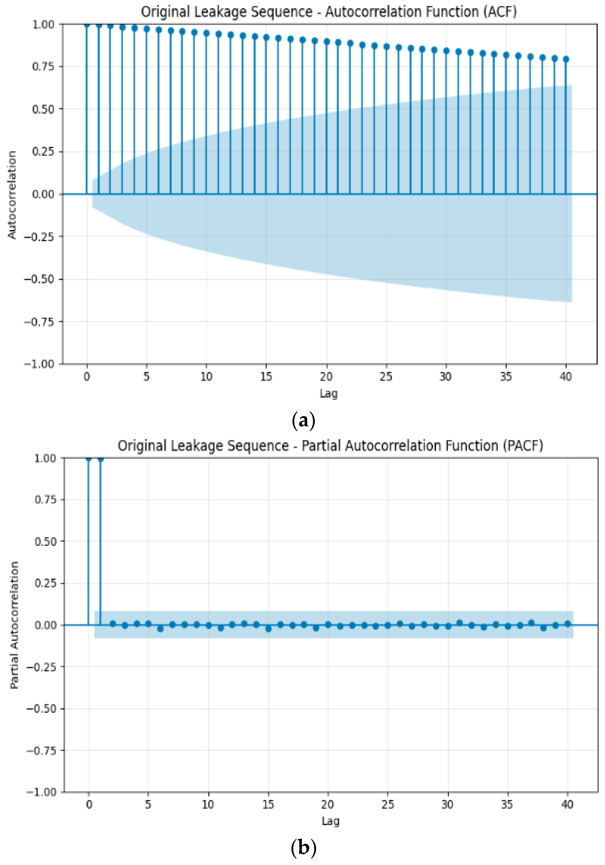
An in-depth understanding of data characteristics is a prerequisite for building accurate prediction models. Visualize and perform statistical analysis on the valve internal leakage time series dataset. Its ACF and PACF plots are shown in Figure 3.
The ACF shows a typical slow decay pattern: the autocorrelation coefficients gradually decrease as the lag order increases but do not show rapid cutoff. This phenomenon is highly related to the unit root process in theory, indicating that the current state of the series has long memory and persistent dependency on its historical states. This suggests the series may have a stochastic trend, and its sample path local behavior exhibits strong random walk characteristics. The PACF shows significant cutoff after the first lag: the partial autocorrelation coefficients drop sharply after lag 1 and remain statistically insignificant. This characteristic usually points to a first-order autoregressive process. However, when slow ACF decay and PACF cutoff after lag 1 occur simultaneously, it strongly suggests a non-stationary AR process with a first-order unit root.
This phenomenon highly aligns with the physical process of initial slight leakage and subsequent accelerated degradation in valve internal leakage, revealing the inherent conditional heteroskedasticity characteristics of internal leakage evolution. Traditional ARMA models are ineffective against this characteristic, which is also the core motivation for introducing the GARCH model in this paper. The proposed IARIMA-GARCH’s core advantage lies in its stepwise modeling strategy: ARIMA component (after differencing) is responsible for capturing and predicting the deterministic trend of the series, the “average growth level” of internal leakage; while the GARCH component dynamically characterizes and predicts the stochastic volatility of the series, the “degree of uncertainty” of internal leakage. This structure allows the model not only to answer “what is the expected future internal leakage” but also to assess “how large is the confidence interval for this prediction”, providing more information for risk perception. To verify the effectiveness of the IARIMA-GARCH method, comparative analyses were also conducted with the ARIMA model and LSTM model.

4.2. Model Construction

(1)
Model Parameter Selection Strategy
When constructing the IARIMA-GARCH model, it is essential to determine its key parameters, such as the optimal orders p and q for the ARIMA and GARCH models, the threshold parameter δ in the Huber loss function, and the volatility feedback coefficient λ introduced in the improved GARCH model. The appropriate selection of these parameters significantly impacts the predictive accuracy of the model, and the specific selection strategies are as follows.
In the process of determining the orders of time series models, both the AIC and the Bayesian Information Criterion (BIC) are commonly used model selection criteria. This study selects AIC as the primary criterion for determining the optimal orders p and q of the ARIMA and GARCH models, based on the following two considerations:
First, the original intention of the AIC is to identify a model that minimizes the Kullback–Leibler divergence from the unknown true data-generating process, to find an approximate model with optimal predictive accuracy. Its formula, A I C = 2 k 2 l n ( L ) , strikes a balance between penalizing the number of parameters ( k ) and rewarding the model’s goodness-of-fit ( l n ( L ) ) , but the penalty is relatively moderate. The core objective of this study is to construct a model with high predictive accuracy for valve internal leakage trends, rather than strictly identifying the true underlying parameter structure of the data. Therefore, AIC’s focus on out-of-sample predictive capability aligns better with the engineering application goals of this research.
Second, from a practical feasibility perspective, the BIC ( B I C = k l n ( T ) 2 l n ( L ) ) tends to select more parsimonious models than the AIC due to its penalty term coefficient l n ( T ) , which increases significantly with sample size T, thus providing stronger model selection consistency. However, in engineering practice fields such as equipment condition monitoring, the dynamic characteristics of the time series may inherently require a slightly more complex model to fully capture its evolutionary patterns. An excessively stringent penalty may lead to underfitting and omission of critical dynamic information. During the preliminary research phase, this study also compared the order selection results of the BIC and found them consistent with those of AIC (for instance, the GARCH(1, 1) model was optimal under both criteria) or only showing minor differences in non-critical parameters. To maintain conciseness and focus in the discussion, the paper uniformly reports the more universally adopted and widely accepted AIC values and their corresponding order selection results in the field of forecasting.
Regarding the threshold parameter δ in the Huber loss function, its value determines the model’s sensitivity to outliers. This study adopts the empirically optimal value of δ = 1.345, which has been rigorously theoretically derived and validated through extensive empirical research in robust statistics. This value is set based on a clear statistical rationale: when the model residuals follow a standard normal distribution, this threshold enables the loss function to maintain efficient least squares estimation for 95% of the valid data (whose residual absolute values are less than or equal to 1.345σ), while applying a linear penalty to the remaining 5% of observations that are potential outliers (whose residual absolute values exceed 1.345σ). This achieves an optimal balance between estimation efficiency and robustness. Adopting this universally recognized value avoids subjective arbitrariness in parameter selection and ensures theoretical rigor and reproducibility of the results of the robustness improvement in the IARIMA model.
As for the volatility feedback coefficient λ introduced in the improved GARCH model, its role is to quantify the intensity of the influence of the conditional volatility from the previous time step on the current residual correction. Since this parameter lacks a prior theoretical optimum and its optimal value is closely related to the volatility characteristics of the specific dataset, this study employs an empirical optimization method for hyperparameters based on grid search. Specifically, on the model training set, a reasonable candidate parameter set (λ ∈ {0.1, 0.2, …, 0.5}) is defined, and model training and validation are performed based on this set. By systematically comparing the comprehensive predictive performance (primarily evaluated using RMSE and MAE) of models with different λ values on a held-out validation set, λ = 0.2 was ultimately selected as the optimal parameter for the model. This selection process is essentially an optimization procedure aimed at minimizing out-of-sample prediction error, ensuring that the determined λ value most effectively adapts to the dynamic volatility structure of the current valve internal leakage sequence, thereby maximizing the synergistic modeling advantages of the improved GARCH model.
(2)
Model construction details
This paper uses four methods, IARIMA-GARCH, ARIMA, LSTM, and XGBoost, for comparative analysis of valve internal leakage prediction. The initial parameters for the four methods are set as follows: the maximum number of iterations is set to 800, the threshold in the combined prediction is set to 1.345, and the parameter for the previous moment’s conditional variance in the residual improvement is set to 0.2.
The Multi-Time-Scale parameters in this study were determined based on equipment operational cycle characteristics and data-driven optimization principles. The short-term sequence length TD = 300 was rigorously optimized and validated; this length fully covers key equipment operational cycles (such as start–stop cycles and load variation cycles), effectively capturing the complete short-term dynamic characteristics. Nk = 3 achieves the optimal balance in moving averages, both effectively suppressing intra-day random fluctuations and completely preserving the medium-term trend characteristics with a “3-day” cycle. Meanwhile, Nj = 5 demonstrates optimal performance in long-term trend extraction, ensuring effective scale separation from the medium-term scale (Nk = 3) while avoiding excessive smoothing caused by overly large windows. If the data volume in the set is not fully divisible, the points farthest from the prediction set and with minimal impact are discarded to achieve the largest multiples of Nk and Nl within the dataset.
The Huber loss function was used to enhance the robustness of the ARIMA model against outliers. To determine the optimal model orders (p, d, q), we first perform a grid search over possible p and q values (with d pre-determined through unit root testing). For each (p, q) combination, we estimate the model parameters using the Huber loss as the objective function and record the corresponding Huber loss score (huber_score). At the same time, AIC was calculated for each model to evaluate model goodness-of-fit and complexity. Ultimately, the model with the smallest Huber loss score and relatively low AIC value was selected as the best model, achieving a balance between robustness and statistical efficiency.
Since the orders corresponding to the short-term, medium-term, and long-term subsequences are different, only the short-term subsequence is used as an example. Its model order selection results are shown in Table 1 and Table 2.
To eliminate non-stationarity, first-order differencing is performed on the series, ensuring the modeling is based on a stationary process. For the ARIMA model, the optimal order (p, q) is determined by comparing the Huber Score across different combinations, as a lower Huber Score indicates superior robustness against outliers. From Table 1, the ARIMA(1, 3) model achieves the lowest Huber Score (0.03661), identifying it as the most robust choice for the short-term subsequence. Therefore, the ARIMA model order (p, d, q) is determined as (1, 1, 3).
Simultaneously, to model the time-varying volatility of the series, the GARCH model order is selected based on the AIC, where a smaller AIC value suggests a better model fit with parsimony. From Table 2, the GARCH(1, 1) model yields the smallest AIC value (1437.5), confirming it as the optimal volatility model. The GARCH(1, 1) model has been widely proven to excellently fit the volatility of most financial and economic time series. This study verifies its applicability in the field of industrial equipment degradation as well. Its “memory effect” means that current volatility is influenced by both past volatility and past disturbances (innovations), which aligns with the physical mechanism of cumulative effects in irreversible processes like metal fatigue and sealing surface damage.
After determining the optimal orders for the ARIMA and GARCH models, to ensure the rigor and reproducibility of the comparative experiments, this study explicitly discloses the core parameter configurations of all baseline models involved in the performance comparison, including LSTM and XGBoost. LSTM network adopts a single hidden layer structure with the number of hidden layer neurons set to 100, uses the tanh activation function, and is trained via the Adam optimizer (with the learning rate set to 0.0005). The model is trained for 150 epochs with a batch size of 32, and a Dropout rate of 0.3 is introduced to suppress overfitting. For XGBoost model, the key parameters include: a maximum tree depth of 8, the number of trees is 300, the learning rate is 0.05, and lag features based on the past 20 time steps are constructed as input. All the aforementioned parameters have been validated through preliminary experiments to ensure that each model is compared fairly under a relatively optimal configuration.

4.3. Evaluation Metrics

To objectively and quantitatively evaluate the prediction performance of the proposed model, this paper uses MAE, RMSE, MAPE, sMAPE, and R2 as evaluation metrics for model accuracy. Among them, MAE and RMSE are used to measure the deviation between the model’s predicted values and the true values; smaller values indicate smaller prediction errors and higher accuracy. MAPE and sMAPE express the prediction error as a percentage of the true value, providing a more intuitive reflection of the relative error size of the prediction results. R2 reflects the goodness of fit of the model; the closer R2 is to 1, the closer the prediction results are to the actual values. Using five metrics overall to evaluate the prediction results allows for a comprehensive assessment of the model’s prediction accuracy and reliability from different perspectives. Their calculation formulas are as follows:
M A E = 1 n i   =   1 n y i y ^ i
R M S E = 1 n i   =   1 n ( y i y ^ i ) 2
M A P E = 1 n i   =   1 n y i y ^ i y i × 100 %
s M A P E = 1 n i   =   1 n y i y ^ i ( y i + y ^ i ) / 2 × 100 %
R 2 = 1 i   =   1 n ( y i y ^ i ) 2 i   =   1 n ( y i y ¯ ) 2
where n represents the number of data points; y i represents the true value of the i-th sample; y ^ i represents the predicted value of the i-th sample; and y ¯ represents the average of all actual values.

4.4. Experimental Platform

The model in this paper was implemented in the PyCharm 2024.1.1 integrated development environment using the Python 3.8 programming language. The computational platform configuration for model training was as follows: 13th Gen Intel(R) Core(TM) i5-13500H (2.60 GHz) processor and NVIDIA GeForce RTX 4050 Laptop 6 GB graphics processor.

5. Results and Discussion

In order to evaluate the predictive performance of the IARIMA-GARCH method, two types of test cases were designed. The first type is In-Distribution (ID) test, where the testing dataset and training data are both on-site actual data, used to verify the performance of the method on data similar to the training data. Another type is Out-Of-Distribution (OOD) test based on noise injection, which overlays different degrees of noise on actual testing dataset to evaluate the method’s generalization ability and robustness.

5.1. In-Distribution (ID) Test

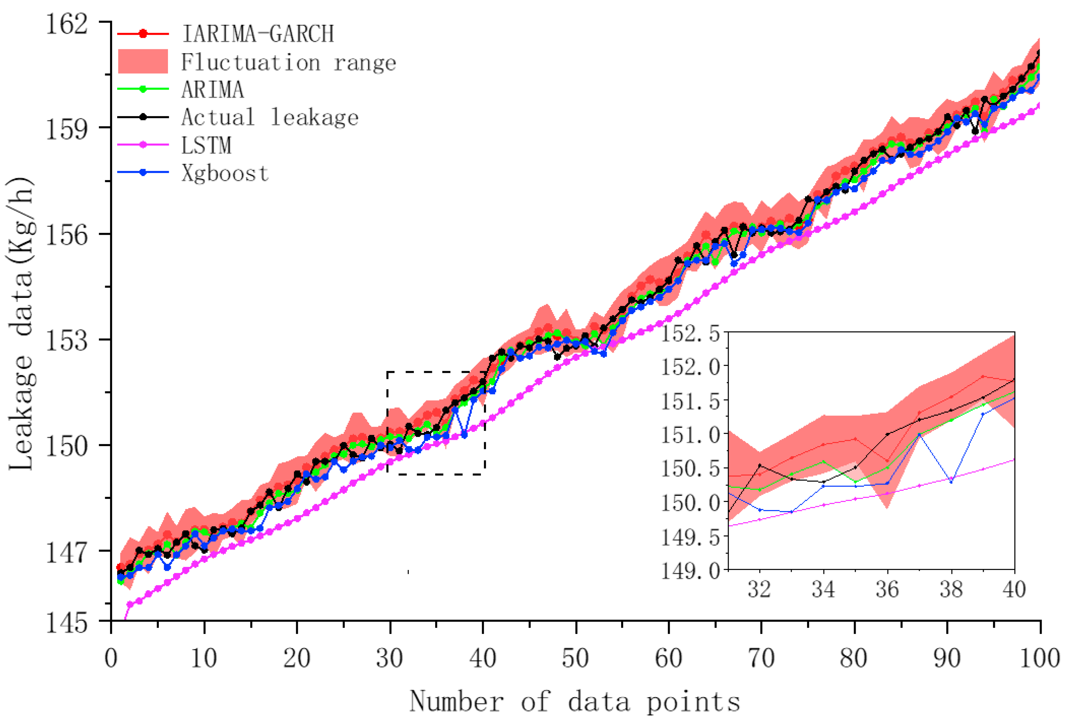
The comparison between the prediction results of the four methods (IARIMA-GARCH, ARIMA, LSTM, and XGBoost) and the actual leakage values on the testing dataset is illustrated in Figure 4. As observed, the actual leakage shows a clear monotonically increasing trend over the data points. The prediction curves of all methods generally follow this upward trend. Among them, IARIMA-GARCH demonstrates the most superior performance. Its prediction curve most closely tracks the actual leakage curve, achieving the highest accuracy. It effectively synergizes the ARIMA model’s capability to determine the series’ growth direction with the GARCH model’s characterization of time-varying volatility. Furthermore, the dynamic fluctuation interval it provides appropriately encompasses the range of the actual values, offering a quantitative basis for risk assessment. This proves that IARIMA-GARCH possesses high application value and reliability for leakage growth warning. In comparison, while the ARIMA model captures the increasing trend after order optimization, its predictions are systematically lower than those of IARIMA-GARCH. Although LSTM and XGBoost can learn complex patterns, their overall prediction performance on this specific dataset with its monotonic increase and smooth trend is inferior to both IARIMA-GARCH and the standard ARIMA model.
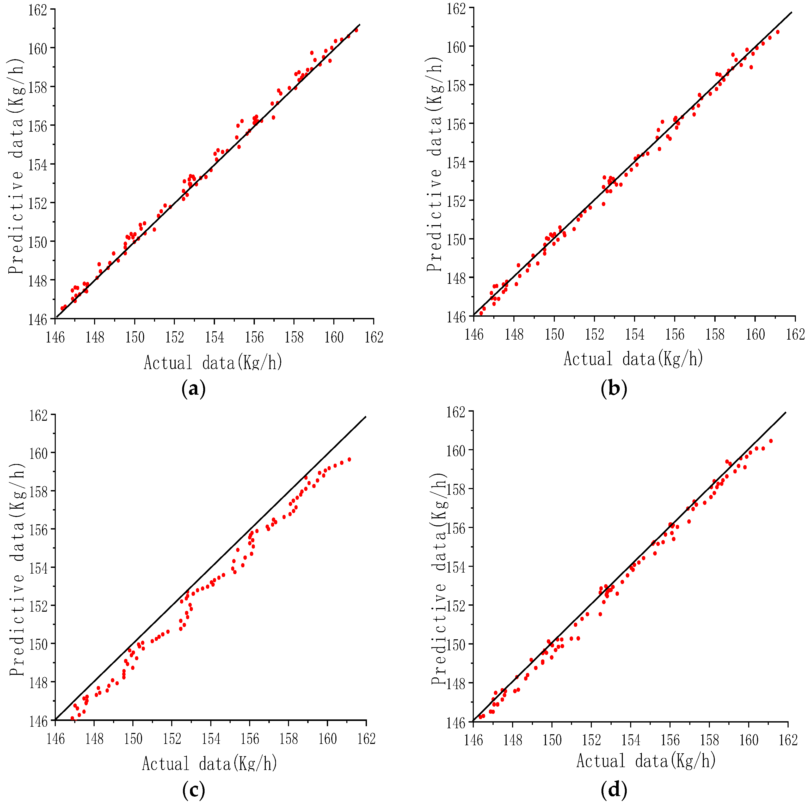
Figure 5 presents a comparative scatter plot of predicted versus actual values across the four methods (IARIMA-GARCH, ARIMA, LSTM, and XGBoost), showing that while all methods generally align along the ideal prediction line, IARIMA-GARCH distinctly outperforms the others, with its points most tightly clustered around the line, demonstrating minimal dispersion and the highest predictive accuracy. In comparison, ARIMA shows noticeable deviations, and both LSTM and XGBoost exhibit even greater scatter, confirming their relatively inferior performance in accurately matching the actual leakage values.
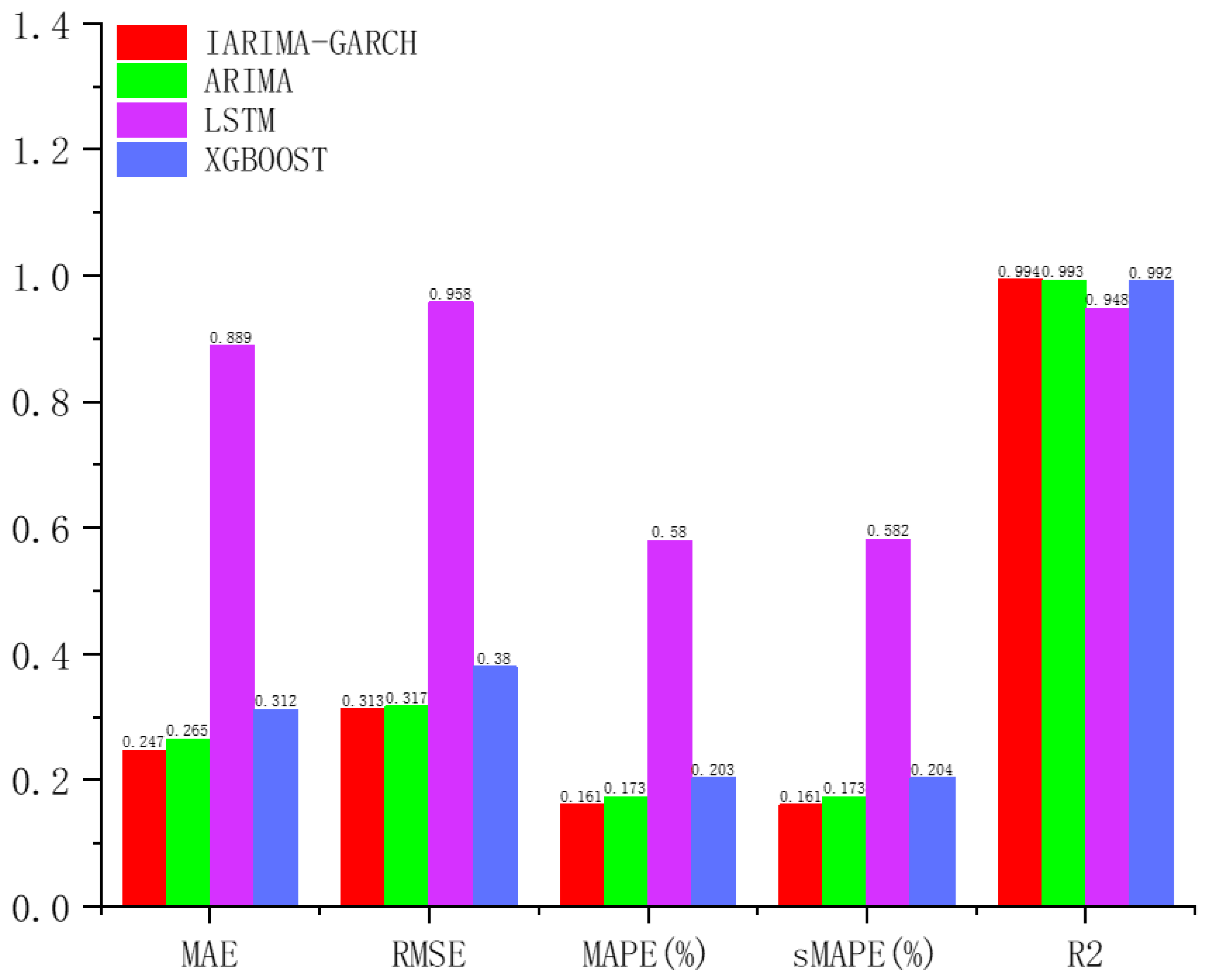
The calculated values of the performance metrics MAE, RMSE, MAPE, sMAPE, and R2 for the four methods are shown in Table 3, and the corresponding performance evaluation bar charts are shown in Figure 6.
Based on the comprehensive performance metrics presented in Table 3 and Figure 6, IARIMA-GARCH demonstrates superior predictive accuracy among the four methods, achieving the lowest error rates across all key indicators—MAE (0.247), RMSE (0.313), MAPE (0.161), and sMAPE (0.161)—along with the highest R2 value (0.994), which confirms its exceptional goodness of fit. In contrast, while the ARIMA model shows relatively strong results with an R2 of 0.993 and moderate error metrics, it is consistently outperformed by IARIMA-GARCH, and both LSTM and XGBoost exhibit significantly higher prediction errors and lower R2 values, highlighting their limitations in capturing the underlying patterns of the valve leakage data. Regarding computational efficiency, ARIMA is the fastest with a training time of only 62 s, benefiting from its linear parametric structure, whereas IARIMA-GARCH requires more time (674 s) due to its two-layer modeling of mean and volatility, a necessary cost for capturing complex time-varying features. LSTM, despite its flexible architecture, incurs the highest computational burden (1743 s) without delivering competitive accuracy, while XGBoost strikes a middle ground in training time (324 s) but fails to match the prediction precision of either IARIMA-GARCH or ARIMA. Overall, these results underscore IARIMA-GARCH as the most accurate and reliable model for leakage prediction, despite its higher computational demand, whereas ARIMA offers a favorable balance of speed and performance for less volatile scenarios. From the perspective of future engineering applications, the scalability of the algorithm is a critical factor to consider. When extending the proposed method to hundreds of valves across an entire plant, the following expansion strategies can be adopted:
(1)
Adopt a parallelized training strategy. Since the model for each valve is independent and the training tasks do not depend on each other, they are highly suitable for embarrassingly parallel processing on computing clusters or cloud platforms. This approach can linearly reduce the overall training time.
(2)
Implement an edge-cloud collaborative architecture. Deploying the trained models at the edge for real-time prediction can significantly reduce the bandwidth and computational pressure on the central system. Model retraining or updates can be performed periodically in the cloud.
(3)
Introduce incremental learning mechanisms. Future work could explore the model’s online learning capability. When new operational data becomes available, instead of performing full retraining, the model parameters could be fine-tuned through incremental update strategies, thereby substantially reducing the computational costs of long-term maintenance.
In summary, although the proposed model introduces additional computational overhead, it demonstrates strong feasibility and scalability for large-scale industrial deployment. The improvement in predictive accuracy, coupled with its robust scalability, will bring significant value to the proactive maintenance of thermal power plants.
Figure 7 shows the normalized performance radar chart of the four methods on the five evaluation metrics. In the chart, the optimal performance for each indicator is normalized to 1, and the area enclosed by the polygon directly reflects the comprehensive performance. The radar chart reveals IARIMA-GARCH’s (red polygon) dominant performance. Its vertices reach the theoretical optimum of 1.0 for every metric, forming the largest polygon area. This indicates an unparalleled, well-rounded optimization with no discernible weakness, excelling in both accuracy (R2) and error minimization. The other methods show a relatively obvious gap compared to it, strongly proving that the superiority of IARIMA-GARCH is comprehensive and robust, rather than a coincidental performance under different evaluation systems.
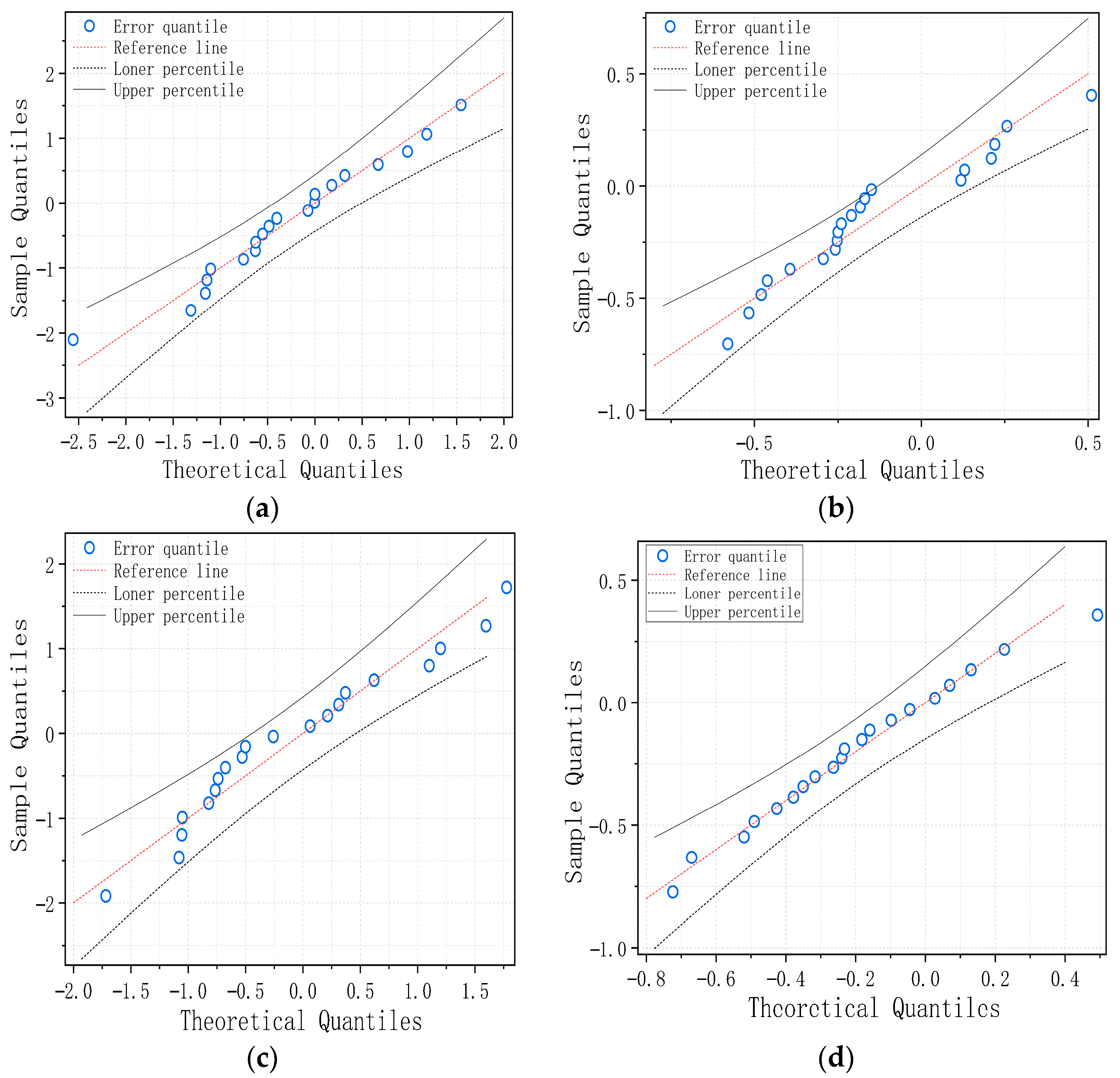
Figure 8 presents the quantile–quantile (Q-Q) plots of the prediction error distributions for the four methods, which are used to assess their conformity to a normal distribution. As shown, the majority of the data points for all methods align approximately along the reference diagonal, suggesting that their prediction errors generally follow a normal distribution. However, noticeable deviations occur at the tails, indicating the presence of outliers or non-normal characteristics, which can impair predictive accuracy, especially for extreme or nonlinear data. Among the four methods, IARIMA-GARCH performs the best, with its points clustering most tightly along the diagonal. In contrast, LSTM shows the most substantial deviations at both tails, followed by XGBoost and then ARIMA. This indicates that the prediction error increases in the following order: IARIMA-GARCH, ARIMA, XGBoost, and LSTM, confirming the superior error distribution and stability of IARIMA-GARCH.
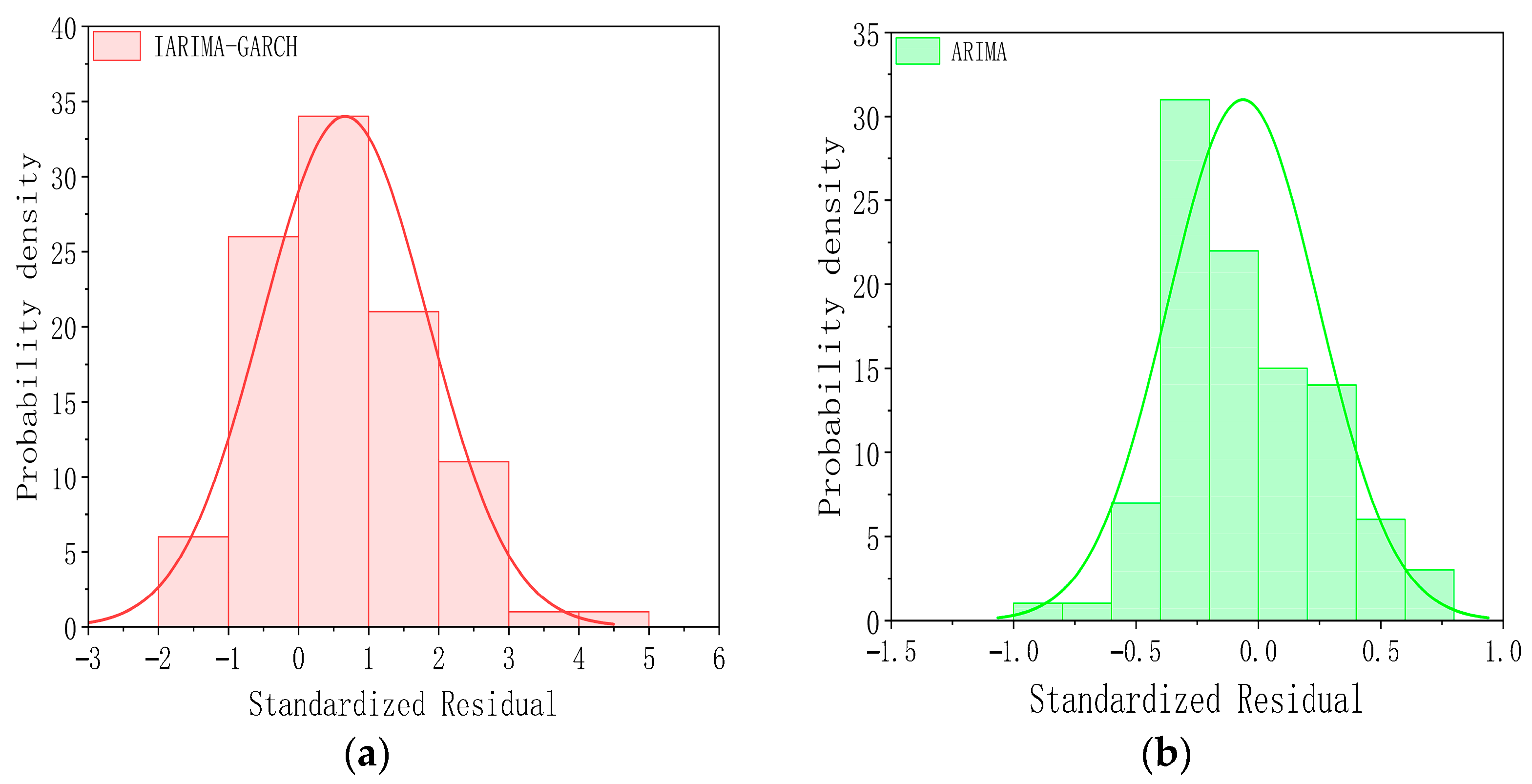
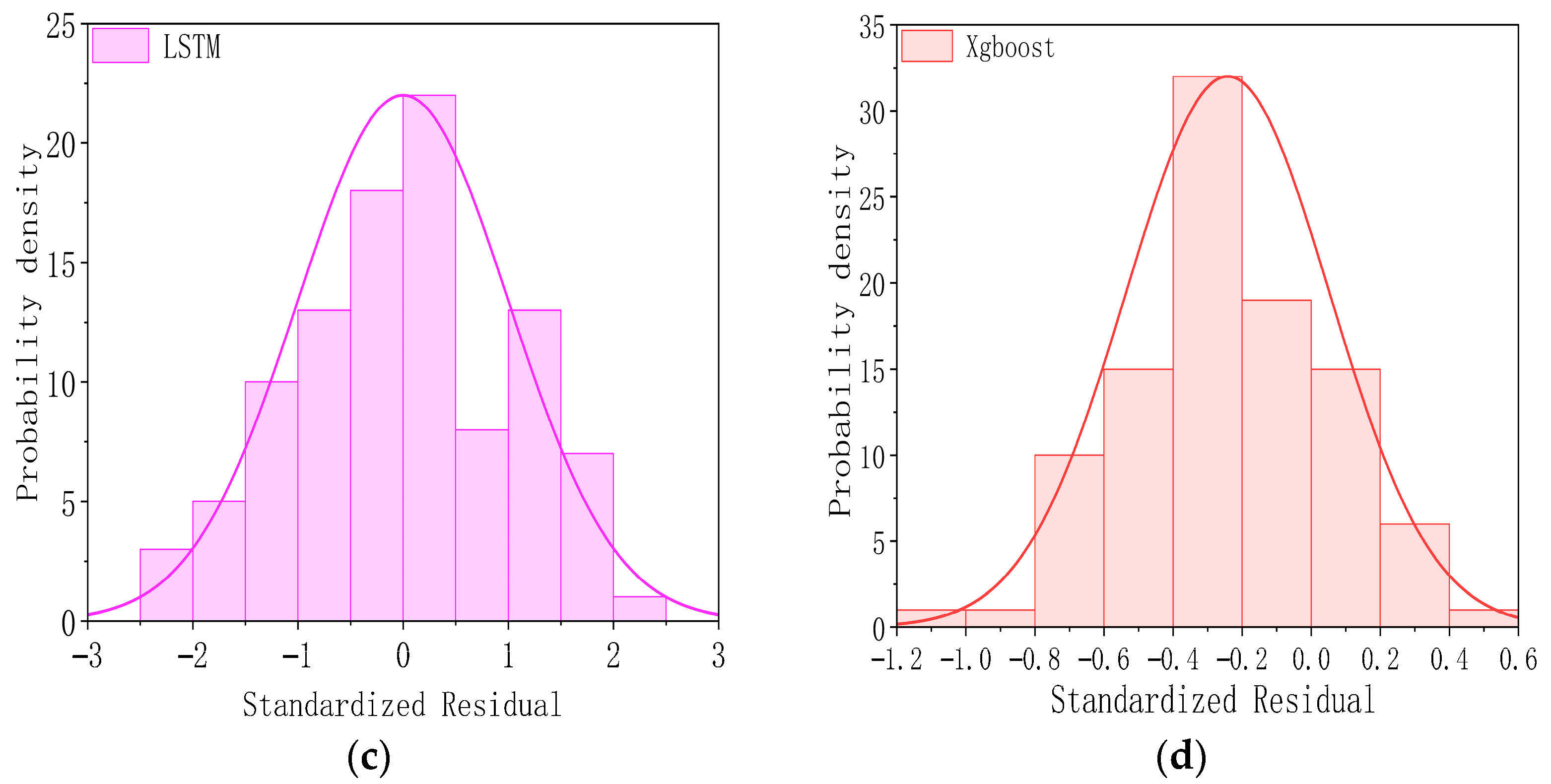
Figure 9 displays the standardized residual histograms with overlaid normal distribution curves for the four methods. The analysis reveals that IARIMA-GARCH exhibits optimal residual characteristics, with its distribution showing remarkable symmetry and a sharp concentration around zero, closely aligning with the normal density curve. This indicates that its residuals best approximate a white noise sequence, satisfying key statistical assumptions. In comparison, ARIMA shows a slightly wider dispersion, while LSTM displays a markedly irregular and dispersed residual distribution. Critically, XGBoost also shows significant deviations and poor normality fitting, performing notably worse than IARIMA-GARCH. The superior residual profile of IARIMA-GARCH confirms its enhanced capability in capturing data patterns while maintaining residual stability, ultimately validating it as the most reliable predictor among the four evaluated methodologies.
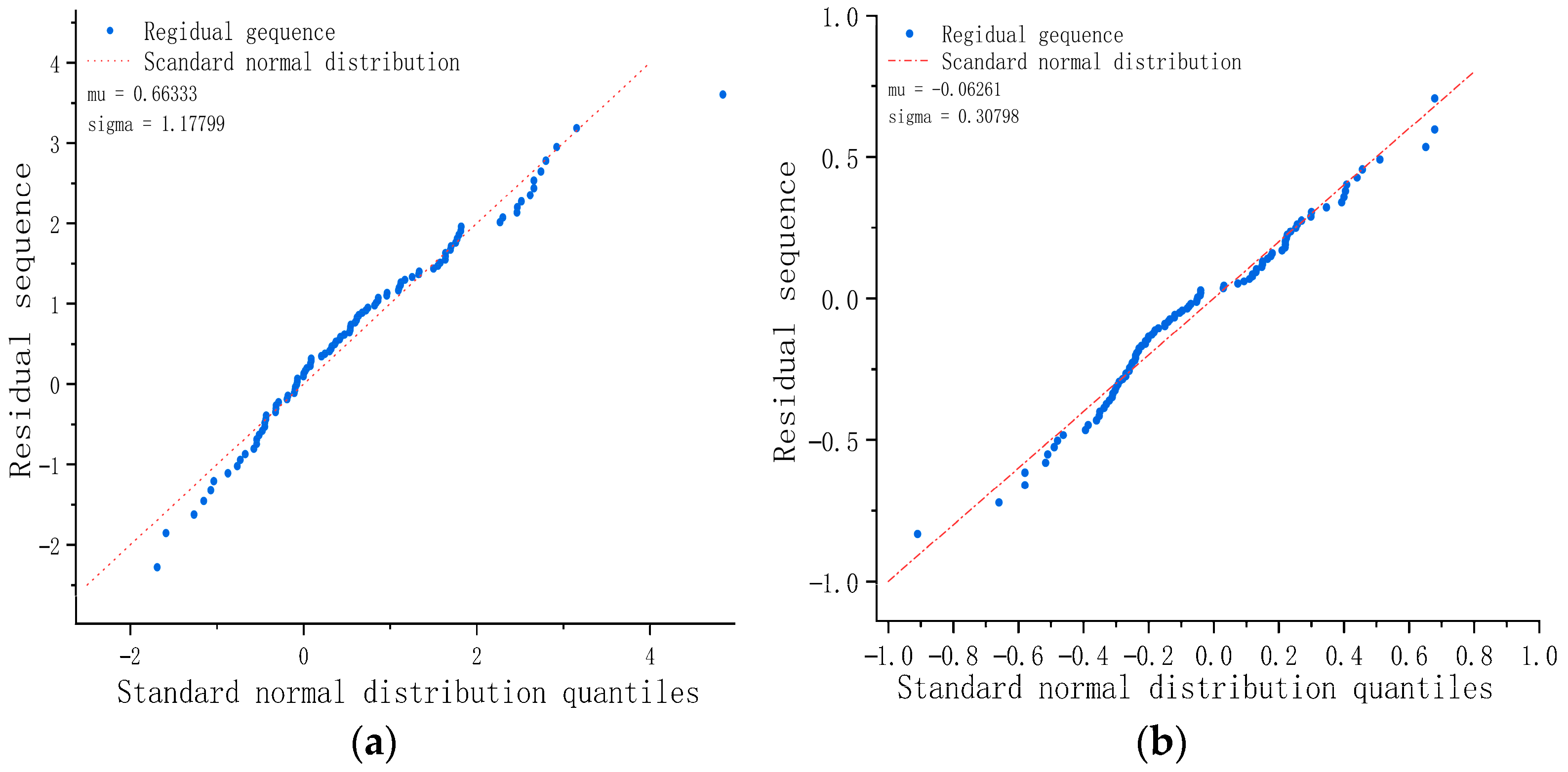
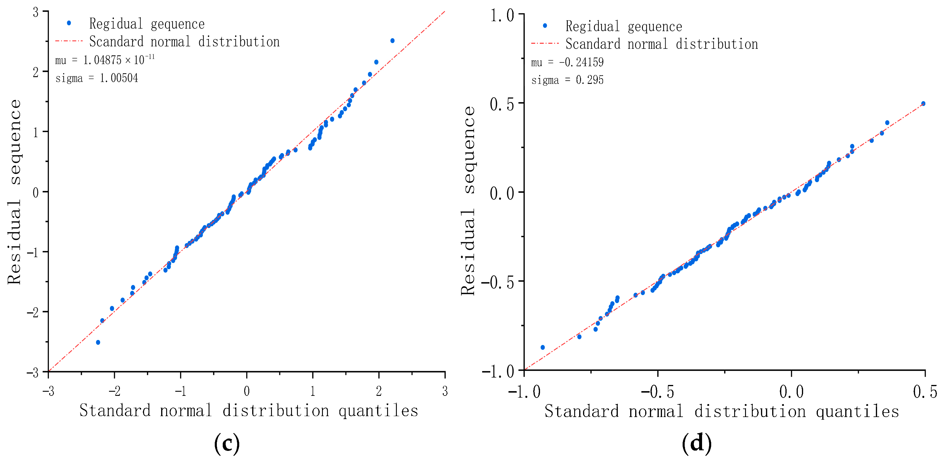
Figure 10 presents the Q-Q plots of standardized residuals for the four methods, providing a rigorous assessment of their residual normality. The analysis demonstrates that IARIMA-GARCH exhibits the most favorable distributional characteristics, with its residuals closely adhering to the theoretical normal distribution line across the entire quantile range. This strong alignment indicates that IARIMA-GARCH’s standardized residuals best satisfy the normality assumption, which enhances the reliability of its statistical inferences and prediction intervals. In contrast, ARIMA, LSTM, and XGBoost all display varying degrees of deviation from normality. Both ARIMA and LSTM show distinct S-shaped curvature in their Q-Q plots, suggesting substantial distributional asymmetry and heavy-tailed characteristics. Notably, XGBoost also exhibits pronounced deviations at both tails, confirming its limitations in achieving proper residual distribution. These systematic deviations from normality in the other three methods undermine the validity of their statistical conclusions and compromise their predictive reliability, thereby reinforcing IARIMA-GARCH’s superior performance in residual diagnostics.

5.2. OOD Test Based on Noise Injection

By incrementally adding white noise to the testing dataset, we systematically simulate data distribution shifts ranging from minor to significant, enabling quantitative analysis of model performance degradation. The OOD test dataset construction method is as follows: Using the testing dataset from Section 5.1 as a baseline, Gaussian white noise is systematically added to input parameter of this dataset to simulate potential data distribution shifts encountered in real-world applications. To ensure noise intensity correlates with the original data scale, the amplitude of white noise is scaled relative to the standard deviation σ j of input parameter in the testing dataset. The white noise level ϵ i , j is incremented α from 0% to 30% in 3% increments, with ϵ i , j following a Gaussian distribution. The noise-augmented testing dataset x t e s t can be expressed as:
x test , i , j   =   x test , i , j + ϵ i , j ,
where x test , i , j represents the original testing dataset, and ϵ i , j denotes white noise, calculated as follows:
ϵ i , j   ~   N ( 0 , ( α / 100 × σ j ) 2 ) .
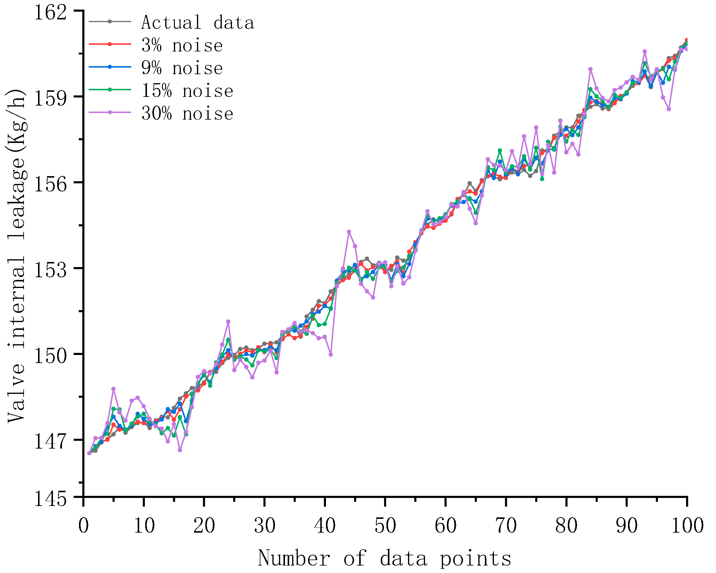
Based on the testing dataset with added noise, the OOD test is conducted on IARIMA-GARCH. The test results for various metrics are shown in Table 4. Taking the scenarios with 3%, 9%, 15%, and 30% added noise as examples, the resulting identification curves are depicted in Figure 11.
As seen in Figure 11, the prediction curves of IARIMA-GARCH closely follow the actual leakage data under various noise levels (3%, 9%, 15%, and 30%). All curves maintain the correct monotonic increasing trend, demonstrating the model’s strong ability to capture core patterns under noisy conditions.
Table 4 provides quantitative support. The R2 remains high, staying above 0.89 even with 30% noise. This shows IARIMA-GARCH keeps a strong explanation of the data trend. All error metrics (MAE, RMSE, MAPE, sMAPE) increase systematically yet gradually as noise rises. When noise stays below 15%, errors grow slowly. Beyond this point, errors increase faster, suggesting a performance boundary. Still, the method continues to provide meaningful predictions even under strong noise.
In summary, the IARIMA-GARCH method shows high robustness against data noise. It reliably tracks long-term trends while GARCH component effectively represents rising uncertainty through dynamic fluctuation intervals. This makes the method highly suitable for real industrial applications with data noise, supporting both accurate leakage warning and quantitative risk assessment.

6. Conclusions

Accurate prediction of valve internal leakage is of great significance for improving the safety and economy of thermal power plant operation. To address the problems of prediction lag and insufficient accuracy in existing methods when dealing with the dynamic changes in internal leakage, this paper proposed the IARIMA-GARCH method to achieve accurate prediction of valve internal leakage. Taking the main steam drain valve of a thermal power plant as the research object, and using MAE, RMSE, MAPE, sMAPE, and R2 as evaluation metrics, a case study and model validation for valve internal leakage prediction were conducted, comparing with the ARIMA, LSTM, and XGBoost methods. The main conclusions of the paper include the following:
(1)
Compared to ARIMA, LSTM, and XGBoost, IARIMA-GARCH has the highest prediction accuracy and is significantly better than the other methods. Its prediction curve has the highest degree of agreement with the actual leakage curve. Its MAE is 0.247, RMSE is 0.313, MAPE is 0.161, and sMAPE is 0.161, which are the smallest among the four methods and significantly lower than the other methods; its R2 is 0.994, very close to 1, and is the highest among the four.
(2)
IARIMA-GARCH can effectively quantify prediction uncertainty and provide reliable prediction intervals. The prediction interval (volatility interval) it outputs can effectively encompass most of the actual leakage data points. This not only proves that the GARCH component successfully captures the volatility clustering of the series but also provides an intuitive and reliable quantitative basis for risk assessment in engineering practice.
(3)
The residuals of IARIMA-GARCH satisfy the statistical assumptions, verifying the completeness of the model specification. From the diagnostic results of the normal distribution plot and Q-Q plot, the standardized residual sequence of IARIMA-GARCH is closest to a white noise sequence with zero mean and unit variance, and its distribution shape is closer to a normal distribution than the other methods. This indicates that it has fully extracted the linear and nonlinear patterns in the series, and there is no significant predictable information left in the residuals, statistically proving the rationality and superiority of the model specification.
In summary, IARIMA-GARCH proposed in this paper not only has a clear mechanism but also possesses high accuracy, strong adaptability, and excellent statistical properties, providing a reliable theoretical tool and practical solution for condition prediction and condition-based maintenance of valve internal leakage.
The case study in this paper is limited to steam drain valves in thermal power plants and has not yet covered other valve types or broader industrial scenarios. Its transferability and industrial robustness still require further validation across different valve types, unit capacity scales, and operational conditions. Future research will focus on expanding the method’s application scope in the following aspects:
(1)
Validation on multiple valve types. The method will be extended to different types of valves such as reheat steam drain valves and extraction steam drain valves at various stages, testing its predictive performance under diverse working conditions including high-pressure/high-temperature, medium-pressure/medium-temperature, and low-pressure/low-temperature environments.
(2)
Testing on units of different capacity classes. The method will be deployed on thermal power units with different capacities (300 MW, 600 MW, 1000 MW) to evaluate its robustness under varying load fluctuations, operational strategies, and equipment aging levels.
(3)
Adaptation to multiple operational conditions. The method’s adaptability under complex operational scenarios such as variable load operation, frequent start–stop cycles, and extreme conditions will be explored. By developing online learning mechanisms to accommodate performance shifts due to equipment aging, and by investigating transfer learning-based methods for rapid cross-domain model adaptation, the method’s generalization ability across different unit capacities and valve types will be enhanced to ensure its reliability across the full range of operating conditions.

Author Contributions

Conceptualization, R.H., L.C. and C.H.; methodology, K.L. and Z.G.; software, Z.G. and X.Y.; validation, Z.G. and C.H.; data curation, R.H.; writing—original draft preparation, L.C. and X.Y.; writing—review and editing, X.Y.; supervision, K.L.; project administration, R.H. and C.H. All authors have read and agreed to the published version of the manuscript.

Funding

This research was funded by the Science and Technology Project of State Grid Shanxi Electric Power Company (Project Name: Online Monitoring and Maintenance Strategy Optimization System for Valve Internal Leakage in Thermal Power Plants; No. 5205ww24000F).

Data Availability Statement

The original data presented in the study are openly available at https://doi.org/10.5281/zenodo.17642266.

Conflicts of Interest

Authors Ruichun Hou, Lin Cong and Kaiyong Li were employed by the company Shanxi Century Central Test Electricity Science & Technology Co., Ltd. The remaining authors declare that the research was conducted in the absence of any commercial or financial relationships that could be construed as a potential conflict of interest. The authors declare that this study received funding from State Grid Shanxi Electric Power Company. The funder was not involved in the study design, collection, analysis, interpretation of data, the writing of this article or the decision to submit it for publication.

Abbreviations

AbbreviationMeaning
ARIMAAutoregressive Integrated Moving Average Model
IARIMAImproved Autoregressive Integrated Moving Average Model
GARCHGeneralized AutoRegressive Conditional Heteroskedasticity
IGARCHImproved Generalized AutoRegressive Conditional Heteroskedasticity
LSTMLong Short-Term Memory
RNNRecurrent Neural Networks
CNNConvolutional Neural Networks
XGBoosteXtreme Gradient Boosting
MPPTMaximum Power Point Tracking
SSASalp Swarm Algorithm
P&OPerturb and Observe
ACFAutocorrelation Function
PACFPartial Autocorrelation Function
ADFAugmented Dickey–Fuller
AICAkaike Information Criterion
BICBayesian Information Criterion
MAEMean Absolute Error
RMSERoot-Mean-Squared Error
R2Determination Coefficient
MAPEMean Absolute Percentage Error
sMAPESymmetric Mean Absolute Percentage Error
ParameterMeaning
N k Number of internal leaks
z t ( d ) the stationary series in the ARIMA model
d dth-order difference operator
B Lag operator
Q t Subsequence set
ρ ^ k Autocorrelation function value
γ ^ k Autocovariance function
γ ^ 0 Time series variance
ς ^ Time series mean
ω t Error term
z t k Lagged Observation
φ k k 1 Regression coefficient
z t ^ Predicted value of a stationary time series at time t
μ Model constant term
ϕ i Autoregressive coefficients of the AR part
θ j Moving average coefficient of the MA part
z t i Lag term of a stationary series
e t j Previous period residual term
e t Residual at time t
δ Huber loss function threshold
ψ δ ( e i ) The derivative of the Huber loss function
H k Step k inverse Hessian approximation
s k Parameter Increment
y k Gradient Increment
ε Convergence tolerance
k m a x Maximum number of iterations
α 0 Assist in regressing the constant term
α i Auxiliary regression coefficient
u t Auxiliary regression error term
TAuxiliary regression sample size
R 2 Coefficient of determination for auxiliary regression
σ t 2 Conditional variance at time t
ω Constant term (intercept)
α i Coefficient of the ARCH term
β j Coefficient of the GARCH term
H ( ω , α 1 , α n ,   β 1 , , β m ) The sun position before mutation
NTotal number of observations
λ Conditional coefficient of variation
E n , t Error metric based on RMSE
N n Number of samples contained in the subsequence
ε ^ A positive number arbitrarily smaller than the normal error

References

  1. Zheng, D.J.; Wang, X.; Yang, L.L.; Li, Y.Q.; Xia, H.; Zhang, H.C.; Xiang, X.M. Review of Acoustic Emission Detection Technology for Valve Internal Leakage: Mechanisms, Methods, Challenges, and Application Prospects. J. Sens. Technol. 2025, 25, 4487. [Google Scholar] [CrossRef] [PubMed]
  2. Jin, T.; Guo, R.Z.; Jia, F.S.; Yuan, X.H.; Guo, Z.H.; He, C.B. Quantitative analysis and influencing factors research on valve internal leakage in thermal power unit. In Proceedings of the 7th Asia Energy and Electrical Engineering Symposium, Chengdu, China, 28 March 2025; pp. 748–753. [Google Scholar]
  3. Elatar, A. Advancements in Heat Transfer and Fluid Mechanics (Fundamentals and Applications). J. Energy Res. 2025, 18, 3384. [Google Scholar] [CrossRef]
  4. Kano, R.; Ryuzono, K.; Date, S.; Abe, Y.; Okabe, T. Structural optimization of composite aircraft wing considering fluid–structure interaction and damage tolerance assessment using continuum damage mechanics. J. Aerosp. Eng. 2025, 167, 110652. [Google Scholar] [CrossRef]
  5. Qamar, M.S.; Munir, M.F.; Waseem, A. AI for Cleaner Air: Predictive Modeling of PM2.5 Using Deep Learning and Traditional Time-Series Approaches. J. Comput. Model. Eng. Sci. 2025, 144, 3557–3584. [Google Scholar] [CrossRef]
  6. Sanchez-Cuevas, P.; Diaz-del-Rio, F.; Casanueva-Morato, D.; Rios-Navarro, A. Competitive cost-effective memory access predictor through short-term online SVM and dynamic vocabularies. Future Gener. Comput. Syst. 2025, 164, 107592. [Google Scholar] [CrossRef]
  7. Haddouchi, M.; Berrado, A. Forest-ORE: Mining an optimal rule ensemble to interpret random forest models. Eng. Appl. Artif. Intell. 2025, 143, 109997. [Google Scholar] [CrossRef]
  8. Liu, S.; Li, C.; Bai, F. PROPHET: PRediction of 5G bandwidth using Event-driven causal Transformer. Proc. ACM Meas. Anal. Comput. Syst. 2025, 9, 35. [Google Scholar] [CrossRef]
  9. Lee, H.; Ahn, Y. Comparative Study of RNN-Based Deep Learning Models for Practical 6-DOF Ship Motion Prediction. J. Mar. Sci. Eng. 2025, 13, 1792. [Google Scholar] [CrossRef]
  10. Song, J.; Liang, R.; Yuan, B.; Hu, J. DIMO-CNN: Deep Learning Toolkit-Accelerated Analytical Modeling and Optimization of CNN Hardware and Dataflow. IEEE Trans. Comput.-Aided Des. Integr. Circuits Syst. 2025, 44, 251–265. [Google Scholar] [CrossRef]
  11. Li, J.; Yang, K.; Wu, Y.; Ye, X.; Yang, H.; Li, X. ProxyMatting: Transformer-based image matting via region proxy. Knowl.-Based Syst. 2025, 310, 112911. [Google Scholar] [CrossRef]
  12. Reisen, V.A.; Lévy-Leduc, C.; Solci, C.C. A robust M-estimator for Gaussian ARMA time series based on the Whittle approximation. J. Appl. Math. Model. 2025, 137, 115712. [Google Scholar] [CrossRef]
  13. Nikolakopoulos, E. Bayesian Semiparametric Multivariate Realized GARCH Modeling. J. Forecast. 2025, 44, 2106–2131. [Google Scholar] [CrossRef]
  14. Sun, J.; Jiang, G.; Jiang, Y.; Li, H.; Zhou, Z.; Liu, Y. A single-sensor leak localization method for high-temperature and high-pressure steam superheater pipes based on VMD-ARMA-SSMUSIC. Appl. Therm. Eng. 2025, 280, 128210. [Google Scholar] [CrossRef]
  15. Xiangxin, X.; Isah, K.O.; Yakub, Y.; Aboluwodi, D. Revisiting the Volatility Dynamics of REITs Amid Uncertainty and Investor Sentiment: A Predictive Approach in GARCH-MIDAS. J. Forecast. 2025, 44, 2193–2204. [Google Scholar] [CrossRef]
  16. Lin, W.; Tian, X. Research on Leak Detection of Low-Pressure Gas Pipelines in Buildings Based on Improved Variational Mode Decomposition and Robust Kalman Filtering. J. Sens. Technol. 2024, 24, 4590. [Google Scholar] [CrossRef] [PubMed]
  17. Li, Y.; Gao, J.; Zhou, J.; Zhu, T.; Jiang, Z. A method of milling force predictions for machining tools based on an improved ARMA model. J. Aircr. Eng. Aerosp. Technol. 2023, 95, 950–957. [Google Scholar] [CrossRef]
  18. Syuhada, K.; Tjahjono, V.; Hakim, A. Improving Value-at-Risk forecast using GA-ARMA-GARCH and AI-KDE models. J. Appl. Soft Comput. 2023, 148, 110885. [Google Scholar] [CrossRef]
  19. Liao, X.C.; Chen, W.N.; Guo, X.Q.; Zhong, J.H.; Wang, D.J. DRIFT: A Dynamic Crowd Inflow Control System Using LSTM-Based Deep Reinforcement Learning. J. Syst. Man Cybern. 2025, 55, 4202–4215. [Google Scholar] [CrossRef]
  20. Liu, K.; Liu, M.Z.; Tang, M.; Zhang, C.; Zhu, J.W. XGBoost-Based Power Grid Fault Prediction with Feature Enhancement: Application to Meteorology. Comput. Mater. Contin. 2025, 82, 2893–2908. [Google Scholar] [CrossRef]
  21. Tang, M.; Meng, C.; Li, L.; Wu, H.; Wang, Y.; He, J.; Huang, Y.; Yu, Y.; Alassafi, M.O.; Alsaadi, F.E.; et al. Fault detection of wind turbine pitch connection bolts based on TSDAS-SMOTE with XGBOOST. Fractals 2023, 31, 2340147. [Google Scholar] [CrossRef]
  22. Xu, Y. Extended Multivariate EGARCH Model: A Model for Zero-Return and Negative Spillovers. J. Forecast. 2025, 44, 1266–1279. [Google Scholar] [CrossRef]
  23. Huang, B.Y.; Song, K.; Jiang, S.L.; Zhao, Z.Q.; Zhang, Z.Q.; Li, C.; Sun, J.W. A Robust Salp Swarm Algorithm for Photovoltaic Maximum Power Point Tracking Under Partial Shading Conditions. Mathematics 2024, 12, 3971. [Google Scholar] [CrossRef]
  24. Bharatheedasan, K.; Maity, T.; Kumaraswamidhas, L.A. Enhanced fault diagnosis and remaining useful life prediction of rolling bearings using a hybrid multilayer perceptron and LSTM network model. Alex. Eng. J. 2025, 115, 355–369. [Google Scholar] [CrossRef]
  25. Ren, S.H.; Lou, X.P. Rolling Bearing Fault Diagnosis Method Based on SWT and Improved Vision Transformer. Sensors 2025, 25, 2090. [Google Scholar] [CrossRef] [PubMed]
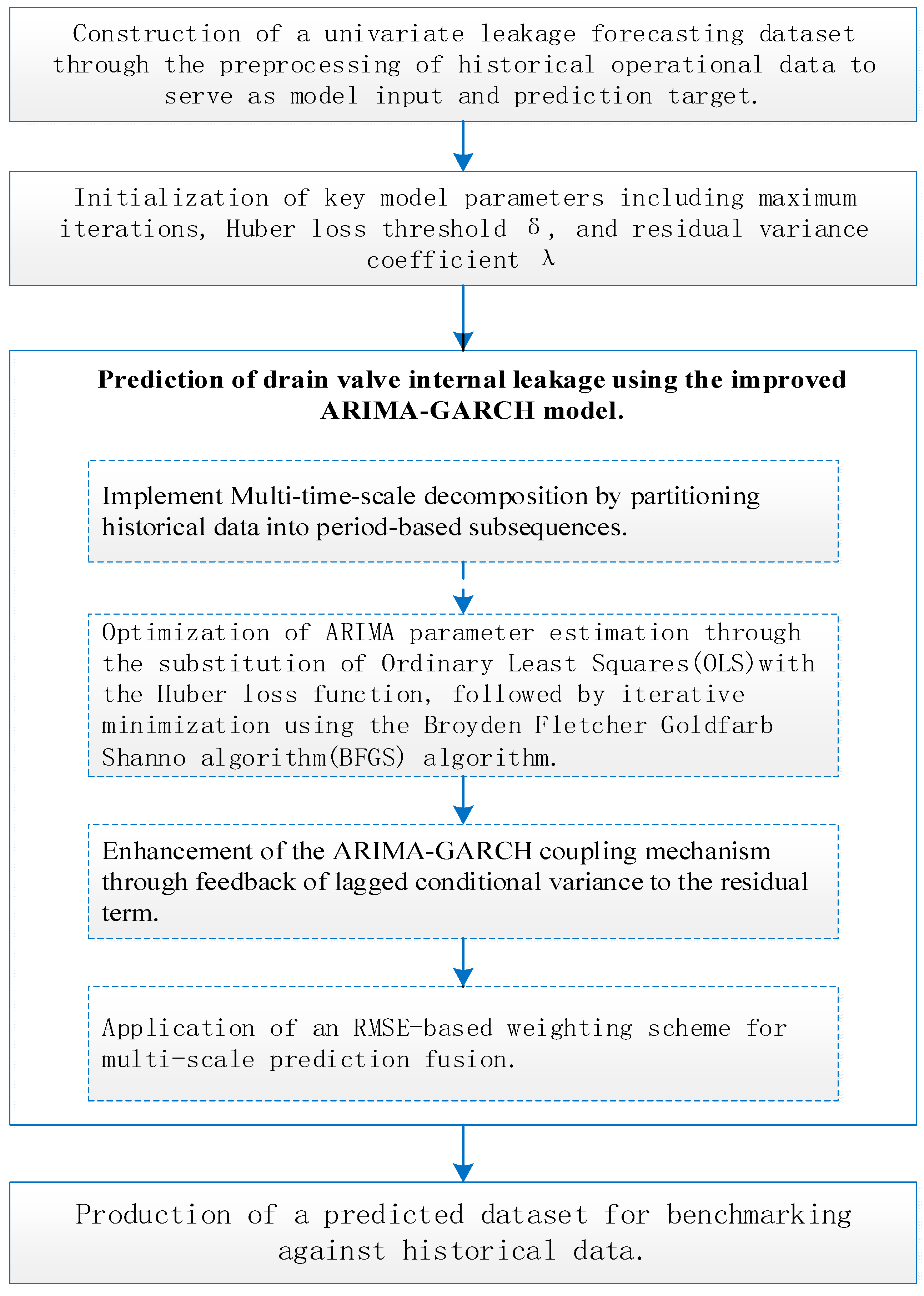
Figure 1. Overall flow chart of IARIMA-GARCH method.
Energies 18 06275 g001
Figure 2. Detailed flow chart of IARIMA-GARCH method.
Energies 18 06275 g002
Figure 3. ACF and PACF plots of the internal leakage time series. (a) ACF plot. (b) PACF plot.
Energies 18 06275 g003
Figure 4. Comparison curves of predicted values and actual values using four methods.
Energies 18 06275 g004
Figure 5. Scatter plots of four methods. (a) IARIMA-GARCH, (b) ARIMA, (c) LSTM, (d) XGBoost.
Energies 18 06275 g005
Figure 6. Bar charts of performance metric values of four methods.
Energies 18 06275 g006
Figure 7. Radar chart of performance metrics of four methods.
Energies 18 06275 g007
Figure 8. Q-Q Plots of prediction errors. (a) IARIMA-GARCH, (b) ARIMA, (c) LSTM, (d) XGBoost.
Energies 18 06275 g008
Figure 9. Standardized residual normal distribution. (a) IARIMA-GARCH, (b) ARIMA, (c) LSTM, (d) XGBoost.
Energies 18 06275 g009aEnergies 18 06275 g009b
Figure 10. Q-Q plots of standardized residuals sequence. (a) IARIMA-GARCH. (b) ARIMA. (c) LSTM. (d) XGBoost.
Energies 18 06275 g010aEnergies 18 06275 g010b
Figure 11. IARIMA-GARCH Identification curves under different noise conditions.
Energies 18 06275 g011
Table 1. Results of ARIMA model selection using Huber Loss.
ModelpqHuber Score
ARIMA(1, 1, 0)100.04062
ARIMA(1, 1, 1)110.03991
ARIMA(1, 1, 2)120.04000
ARIMA(1, 1, 3)130.03661
ARIMA(2, 1, 0)200.04011
ARIMA(2, 1, 1)210.04004
ARIMA(2, 1, 2)220.03998
ARIMA(2, 1, 3)230.06410
Table 2. Results of AIC calculation.
ModelmnNumber of ParametersAIC
GARCH(1, 1)1191437.5
GARCH(1, 2)12101439.9
GARCH(2, 1)21101439.6
GARCH(2, 2)22111437.9
Table 3. Performance metric values of four methods.
MAERMSEMAPEsMAPER2Time (s)
IARIMA-GARCH0.2470.3130.1610.1610.994674
ARIMA0.2650.3170.1730.1730.99362
LSTM0.8890.9580.5800.5820.9481743
XGBoost0.3120.3800.2030.2040.992324
Table 4. OOD test results for metrics of IARIMA-GARCH.
White Noise RatioR2MAERMSEMAPEsMAPE
0%0.99430.24650.31340.16100.1608
3%0.99370.25370.32790.16570.1656
6%0.99010.34670.42610.22650.2263
9%0.98340.45290.55340.29580.2955
12%0.97580.53440.65800.34880.3485
15%0.96500.65090.79450.42500.4247
18%0.95570.72630.90270.47400.4736
21%0.94330.82551.03150.53920.5386
24%0.93120.91181.14350.59490.5944
27%0.90641.08551.34710.70990.7092
30%0.89281.15781.44290.75670.7557
Disclaimer/Publisher’s Note: The statements, opinions and data contained in all publications are solely those of the individual author(s) and contributor(s) and not of MDPI and/or the editor(s). MDPI and/or the editor(s) disclaim responsibility for any injury to people or property resulting from any ideas, methods, instructions or products referred to in the content.