A Deterministic Assurance Framework for Licensable Explainable AI Grid-Interactive Nuclear Control

Abstract

Deploying deep reinforcement learning (DRL) in safety-critical nuclear control is limited less by raw performance than by the absence of licensable, audit-ready evidence. We introduce a Deterministic Assurance Framework (DTAF) that converts controller behavior into licensing-grade proof by combining the following: (i) deterministic licensing gates tied to formal safety and performance limits (e.g., Total Time Unsafe (TTU) = 0; bounded Transient Severity Score (TSS); and minimum Grid Load-Following Index (GLFI)); (ii) a portfolio of adversarial stress tests representative of off-nominal operation; and (iii) a traceability and explainability package that renders every evaluated action auditable. The DTAF is demonstrated on a high-fidelity pressurized-water-reactor (PWR) simulation model used as a software-in-the-loop testbed. Three governor architectures are evaluated under identical, fixed scenarios: a curriculum-trained Soft Actor–Critic (SAC) agent, and Differential-Evolution-optimized Proportional–Integral–Derivative (PID-DE) and Fuzzy-Logic (FLC-DE) Controllers. Performance is assessed deterministically via gate-aligned metrics—TTU, TSS, GLFI, cumulative control effort (CE_sum), valve-reversal count (V_rev), and speed overshoot (OS_ω). Across the adversarial portfolio, the SAC controller meets the predeclared licensing gates in single-run evaluations, whereas the strong conventional baselines violate gates in specific high-severity cases; where all methods remain within the safe envelope, the SAC delivers a higher GLFI and lower CE_sum, with fewer reversals and reduced overshoot. All licensing conclusions derive from deterministic single-run tests; a small, fixed-seed check (three seeds with descriptive intervals) is reported separately as non-licensing supplementary analysis. By producing transparent, reproducible artifacts, the DTAF offers a regulator-oriented pathway for qualifying DRL controllers in grid-interactive nuclear operations.

1. Introduction

Deep reinforcement learning (DRL) has great potential to improve nuclear reactor control performance, especially for load-following in Pressurized Water Reactors (PWRs). However, a major gap separates this potential from practical deployment: current DRL controllers cannot be licensed under today’s nuclear safety regulations. The U.S. Nuclear Regulatory Commission (NRC) and others have identified verification and validation (V&V), trustworthiness, and assurance as the primary hurdles to adopting AI-based control in safety-critical nuclear systems [1,2]. In essence, black-box control policies that lack deterministic, auditable guarantees are disqualified from licensing. PWR grid load-following demands extremely high reliability and predictability—yet DRL agents, despite their technical prowess, pose a regulatory stalemate without a suitable testing and assurance protocol. The missing piece is an auditable deterministic test protocol that can demonstrate an AI controller’s safety to licensing authorities beyond any statistical doubt.

To address this barrier, we propose a Deterministic Assurance Framework (DTAF) tailored for licensing-grade evaluation of AI controllers. The DTAF introduces the following: (i) explicit deterministic licensing gates tied to hard safety limits (for example, preventing frequency trips and bounding speed overshoot OS_ω within allowable margins); (ii) an adversarial stress-test portfolio comprising worst-case grid disturbances and transients designed to probe the controller’s safety envelope; and (iii) a comprehensive traceability and explainability package (integrating eXplainable Reinforcement Learning, XRL) that produces human-interpretable evidence of the controller’s decisions. Under the DTAF, an AI governor must provably keep all key performance indicators within pre-defined deterministic limits during these stress tests. The framework thereby transforms black-box DRL behavior into a licensable pipeline of quantitative gates, stress scenarios, and explainable artifacts that regulators can audit.

We demonstrate the DTAF using a high-fidelity PWR digital model (DM) as a realistic simulation testbed. Three governor controllers are evaluated under identical conditions: a Soft Actor–Critic (SAC) DRL agent, a PID controller optimized by Differential Evolution (PID-DE), and a Fuzzy-Logic Controller optimized by Differential Evolution (FLC-DE). The evaluation metrics include the Total Time Unsafe (TTU), Transient Severity Score (TSS), Grid Load-Following Index (GLFI), cumulative control effort (CE_sum), valve reversal count (V_rev), and speed overshoot (OS_ω). Each metric is mapped to a specific licensing gate with a fixed threshold. For example, the TTU must remain zero for all protected variables, the TSS must not exceed defined severity limits, and the GLFI must stay above minimum grid-following requirements. By design, if any single gate is violated in a test scenario, the candidate controller is disqualified—a stringent criterion aligned with nuclear safety standards.

Our research addresses three core questions under this deterministic protocol: (Q1) Can the SAC agent meet all deterministic licensing gates across an array of adversarial grid disturbance scenarios? (Q2) How do the SAC’s safety, robustness, and performance compare to the PID-DE and FLC-DE baselines under identical stress conditions? (Q3) Can the integrated XRL traceability package explain the SAC’s control actions during severe transients in a way that supports regulatory auditability? To ensure absolute clarity, we declare upfront that all evaluations are fully deterministic. Every stress-test scenario is run in a non-stochastic manner with fixed initial conditions and no random disturbances. The only exception is an auxiliary robustness check (Section 4.10) where we repeat tests with three different fixed random seeds to compute descriptive 95% confidence intervals—and even there, the seeds are predetermined for reproducibility. Crucially, all licensing conclusions in this paper are drawn solely from deterministic results, not from any statistical or probabilistic analysis.

In summary, this work offers three main contributions. (1) We develop the Deterministic Assurance Framework (DTAF)—a regulator-aligned evaluation framework that combines deterministic performance gates, adversarial stress scenarios, and XRL-based traceability into a unified, licensable test pipeline. (2) We present a comprehensive benchmark comparison of a state-aware SAC controller against optimally tuned conventional controllers (PID-DE and FLC-DE) on a high-fidelity PWR simulation model, using identical operating conditions and disturbance scenarios for a fair, rigorous assessment. (3) We provide a complete reproducibility and audit package for public release (containing all training scripts, configuration files, logged time series, and agent checkpoints), enabling independent validation of results. Together, these contributions demonstrate a viable path to make DRL controllers licensable for grid-interactive nuclear plant control by design—resolving the DRL licensing barrier through determinism, stress-testing, and explainability.

2. Related Work

2.1. Reinforcement Learning in Nuclear, Power, and Turbomachinery Control (2019–2025)

In recent years, researchers have explored DRL-based control across nuclear and energy domains to test feasibility. In the nuclear sector, deep RL agents have been applied to reactor operation tasks with encouraging results. For example, Gong et al. survey numerous implementations and conclude that RL can handle complex multi-objective control scenarios in nuclear power plants [3]. Specific case studies have demonstrated that DRL governors can perform continuous reactor coolant and power regulation while meeting multiple objectives [4]. Even microreactors—compact reactors with fast dynamics—have seen prototype RL controllers achieving improved load-following performance over baseline PID tuning [5]. Similarly, in the broader power and turbomachinery arena, DRL techniques have shown promise. A notable example is the use of multi-agent deep RL to optimize boiler–turbine control systems, where adaptive RL-tuned PID policies outperformed conventional tuning in managing a nonlinear multi-input system [6]. These works collectively indicate that DRL can indeed learn effective control policies for complex energy systems. However, they stop at demonstrating performance and do not furnish the licensing-grade evidence (deterministic guarantees, formal safety checks, etc.) that regulators require. In other words, while DRL feasibility in nuclear and turbomachinery control has been established in the 2019–2025 literature, none of these studies deliver the audit-ready determinism or comprehensive safety assurance needed for actual deployment.

2.2. Safety-Aware, Constrained, and Robust RL; Adversarial Evaluation

Concurrently, the DRL research community has developed various techniques to enhance the safety and robustness of learning agents, as well as methods to adversarially test them. One line of work focuses on constrained and safe RL algorithms that enforce safety criteria during training. For instance, Sun et al. propose a chance-constrained RL controller for power plant supervision that uses Lagrange multipliers to strictly respect state constraints (e.g., reactor thermal limits) throughout the learning process [7]. Such approaches embed nuclear engineering knowledge (safety setpoints and margins) directly into the RL optimization, yielding agents that never experience unsafe excursions even while exploring. Another important direction is the adversarial stress-testing of RL policies. Here, the idea is to actively generate worst-case scenarios to probe an agent’s reliability. In the autonomous driving domain, Feng et al. demonstrate a “dense” deep-RL approach that trains adversarial background agents to expose rare failure modes of a vehicle’s policy [8]. This concept—using AI to test AI—highlights how critical safety scenarios can be systematically uncovered. Despite these advances in safe RL and adversarial evaluation, few efforts have integrated them into a unified, regulator-oriented pipeline. In prior nuclear control studies, RL controllers were typically evaluated on nominal or randomly sampled scenarios, rather than an exhaustive set of adversarial drills. Moreover, while robust RL algorithms can limit certain risks (e.g., by adding noise or using domain randomization), regulators ultimately demand deterministic evidence of safety. To date, there is no standard framework in the nuclear domain that combines constrained RL training, adversarial scenario generation, and formal gate-checking of results. Our work fills this gap by incorporating safety constraints and adversarial tests within the DTAF’s deterministic evaluation regime.

2.3. Explainability and Traceability for Deep RL

As DRL agents make increasingly complex control decisions, explainability and traceability have become critical for acceptance in safety-critical systems. The subfield of eXplainable RL (XRL) has produced a variety of techniques to interpret an agent’s behavior [9]. These include feature local sensitivity methods, which highlight the most influential state variables behind an action (e.g., identifying that a reactor RL agent mainly responds to power level and fuel temperature deviations), and policy simplification methods such as surrogate modeling or rule extraction, which approximate the agent’s policy with a human-readable model. For instance, one can train a simple decision tree or linear model to mimic the DRL policy locally, thereby revealing the policy’s decision logic in specific scenarios. Another approach is behavioral cloning or trajectory analysis, where the RL agent’s state-action trajectories under various disturbances are recorded and compared to those of classical controllers to pinpoint differences in strategy. In the nuclear domain, initial steps have been taken to apply XAI techniques for operator support—for example, M. Najar and X. Wang develop explainable AI models to aid reactor operators during accidents [10]. However, achieving full traceability of a DRL controller’s decisions under extreme transients remains an open challenge. Most XRL studies to date focus on either relatively simple environments or post-hoc visualization tools, often divorced from formal verification needs. In our framework, explainability is not an afterthought but a built-in component: the DTAF’s traceability package generates artifacts (such as annotated time-series plots, policy local sensitivity maps, and scenario-wise action comparisons) that accompany each stress-test result. This ensures that for every deterministic pass/fail outcome, there is a corresponding human-interpretable explanation. By aligning XRL techniques with the adversarial test scenarios, we aim to make the DRL agent’s behavior transparent and auditable—satisfying the regulator’s need to know why the AI acted as it did, especially in borderline conditions near safety limits.

2.4. High-Fidelity Simulation Models (Digital Models) for Nuclear/Power Control

High-fidelity simulation models, also referred to as digital models (DMs), serve as indispensable tools for developing and validating control logic in nuclear and power systems. These models emulate the real plant’s physics with sufficient detail to capture transient behaviors, making them ideal for rigorous software-in-the-loop testing. In our context, a PWR simulation DM is used as the core testbed within the DTAF to evaluate all controllers under identical conditions. The advantage of a DM is that extreme scenarios—including rapid load ramps, large disturbances, and equipment faults—can be safely executed and repeated deterministically. Researchers have increasingly employed such digital platforms for AI-driven control studies. For example, Lim et al. describe a high-fidelity PWR simulation framework to train and test an RL-based supervisory controller for advanced reactors [11]. By leveraging a detailed simulator of a Generation-IV plant, they could evaluate the RL agent’s long-term performance and maintenance decisions without any risk to real equipment. In general, DMs allow controllers to be stress-tested in silico against scenarios that might be too dangerous or rare to test on actual reactors or turbines. This not only accelerates development but is also a pre-requisite for licensing—regulators will not consider AI control strategies that have not been thoroughly vetted on validated simulation models. Today, such evaluations are typically confined to software-in-the-loop experiments, but the same models can be extended to hardware-in-the-loop setups (e.g., connecting the simulator to physical controller hardware or plant interfaces) under the DTAF methodology. The key point is that the DTAF’s deterministic protocol is model-agnostic: it can be applied on any high-fidelity DM to produce evidence (logs, safety gate outcomes, and traceability reports) that is replayable and reviewable. This approach ensures that by the time an AI controller is a candidate for on-site trials, it comes with a complete simulation-backed safety dossier. In summary, high-fidelity DMs act as the proving ground where modern control algorithms can earn trust by demonstrating compliance with all operational limits and safety requirements in a virtual yet realistic environment [12,13].

2.5. Comparative Synthesis and Benchmark Rationale

Our study synthesizes insights from the above strands into a cohesive assurance framework, with an emphasis on comparing DRL against strong conventional baselines. In commercial reactor operations, traditional controllers like PID and fuzzy logic remain the dominant solutions due to their stability and regulatory acceptance [14,15]. Over the past decade, many researchers have improved these classical controllers using modern optimization techniques (genetic algorithms, particle swarm, and differential evolution) to enhance performance for complex reactor maneuvers [14,15]. Despite this, prior RL works in nuclear control have rarely, if ever, pitted a DRL agent against an equally well-tuned classical controller under stress conditions. Most feasibility studies compared RL to either a default PID or no baseline at all, leaving open the question of whether the AI truly excels beyond what a properly optimized conventional controller could do. By contrast, we adopt the “Strong Benchmark” philosophy: the SAC agent must demonstrably surpass a PID-DE and FLC-DE that have been optimized across many scenarios. This stringent baseline provides a higher confidence threshold for safety-critical acceptance—an AI that only matches a mediocre controller would not justify the licensing risk. Furthermore, our work combines safety, robustness, and explainability in one deterministic framework, whereas previous research typically addressed these aspects in isolation. For instance, some studies incorporate safety constraints or robust training, and others propose XAI methods, but none have unified them into a single pipeline oriented toward regulator review. It is worth noting that we do not include advanced model-based controllers like MPC or H∞ in our benchmarks; this is a deliberate choice to keep the evaluation controller-centric. While methods such as MPC can yield excellent performance, they introduce model-dependent tuning and complexity that are beyond our scope—our focus is on comparing a learning-based policy with human-engineered policies under identical conditions. Importantly, excluding MPC/H∞ also reflects practical considerations: nuclear plants today still rely on PID-family controllers [14], so demonstrating AI superiority over this familiar baseline is a more direct and convincing argument for stakeholders. Finally, we emphasize that our DTAF approach aligns with formal safety expectations. Nuclear design standards like IAEA No. SSR-2/1 (Rev. 1) mandate that all operational transients remain within defined, bounded limits [12], and software safety guidelines (IAEA Safety Standards Series No. SSG-39) stress the importance of deterministic behavior in systems important to safety [13]. However, as a recent review pointed out, most AI control research lacks comprehensive adversarial validation frameworks to ensure these criteria are met [16]. By integrating optimized baseline comparisons, adversarial scenario testing, and XRL-driven transparency, we provide a template for deterministic assurance that addresses this gap. In short, our benchmark rationale and synthesis highlight the novelty of the DTAF: it is not about pushing an RL agent in isolation but about proving that the agent can reliably and explainably beat the best conventional solutions under the exacting conditions regulators care about.

2.6. Rationale for Differential Evolution (DE) in Strong Baseline Optimization

We adopt Differential Evolution (DE) to optimize the Proportional–Integral–Derivative (PID) and Fuzzy-Logic Controller (FLC) baselines, so that the conventional comparators in the Deterministic Assurance Framework (DTAF) are truly “strong.” DE is a derivative-free, population-based global optimizer with few hyperparameters; it is simple to implement and reproduce, and it is effective on nonconvex, multimodal, and noisy or piecewise-discontinuous closed-loop objectives typical of controller tuning [17,18,19]. Strategy-adaptive DE variants further improve robustness across heterogeneous problems [20], and large comparative studies show DE variants to be highly competitive—often superior on average—to Particle Swarm Optimization (PSO) across numerical benchmarks and real-world tasks [21]. In power-system control specifically, DE has been applied successfully to tune load-frequency and governor-related controllers, providing a domain-proximal precedent for our use in baseline construction [22]. Alternative optimizers are less suitable for our gate-aware objective: exhaustive grid searches are inefficient in high-dimensional, constrained spaces; gradient-based methods require smoothness and reliable derivatives that closed-loop plants and penalty-augmented objectives generally lack; and Bayesian optimization introduces surrogate-modeling overhead and typically needs specialized treatments for heteroscedastic/noisy evaluations—factors that complicate transparency and reproducibility for licensing evidence [23,24]. In the DTAF, we formulate a composite cost that aggregates the licensing metrics—the Total Time Unsafe (TTU), Transient Severity Score (TSS), Grid Load-Following Index (GLFI), cumulative control effort (CE_sum), valve-reversal count (V_rev), and speed overshoot (OS_ω)—with hard (infinite) penalties for any gate violation and soft penalties within the safe envelope. For comparability, the population size, mutation factor, crossover rate, and generation budget are fixed across governors; all settings and seeds are released with the reproducibility package.

3. Methodology

3.1. Plant Simulation Environment

We model a Pressurized Water Reactor (PWR) as a deterministic, single-loop surrogate coupling six-group point kinetics, lumped thermal–hydraulics, a first-order valve servo with rate limiting, a first-order turbine path, and a synchronous generator tied to an infinite bus. The overall architecture and signal flow are shown in Figure 1 and Figure 2, respectively. All symbols are defined at point of use; all parameter values appear in-section to ensure exact reproducibility.

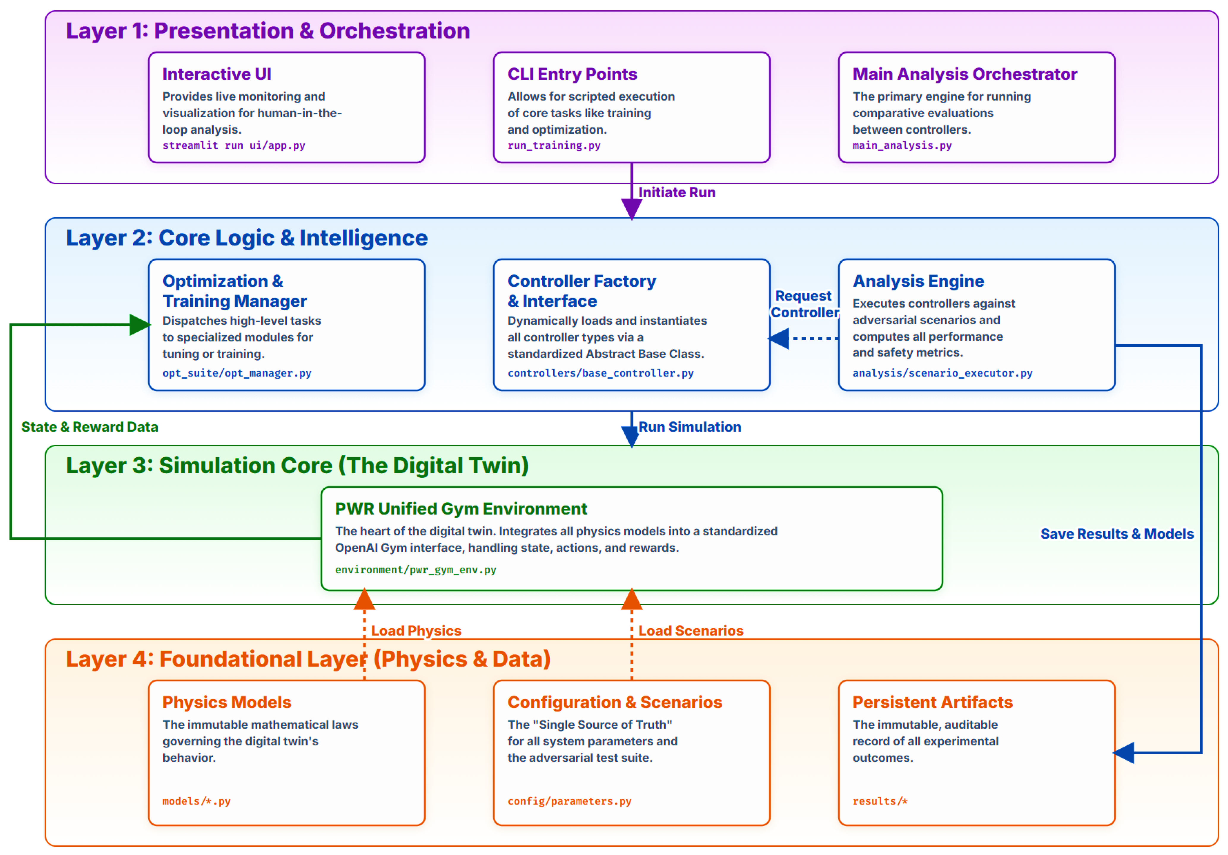
Figure 1 illustrates the complete architecture of the proposed Deterministic Assurance Framework (DTAF), which is engineered to rigorously train, test, and formally verify AI controllers within a safe, high-fidelity simulation environment. The framework is structured as a four-layer hierarchy, with each layer encapsulating a distinct set of functions. At the core, Layer 4 (agent) comprises the Soft Actor-Critic (SAC) reinforcement learning controller, which is responsible for generating real-time control commands, or actions. The agent interacts directly with Layer 3 (environment), the PWR-simulation model, which is wrapped in a PWR Unified Gym Environment interface. This environment executes the agent’s action, calculates the resultant system dynamics, and returns the new state vector and a scalar reward signal, thus closing the standard RL feedback loop. This core loop is governed by Layer 2 (The Analysis Engine), which orchestrates the entire experimental and validation process. This layer is responsible for executing the suite of adversarial stress tests, performing multi-run robustness checks, and conducting the explainability (XAI) analyses required to interpret the agent’s decision-making logic.

Finally, Layer 1 (The Deterministic Assurance Engine) serves as the highest level of oversight. It defines the formal safety and control objectives, such as the operational limits for grid frequency (f_trip) and average reactor temperature (T_avg). This engine performs the ultimate safety verification, systematically ensuring that all agent-driven behaviors, even under stress, remain within the pre-defined safe operating envelope.

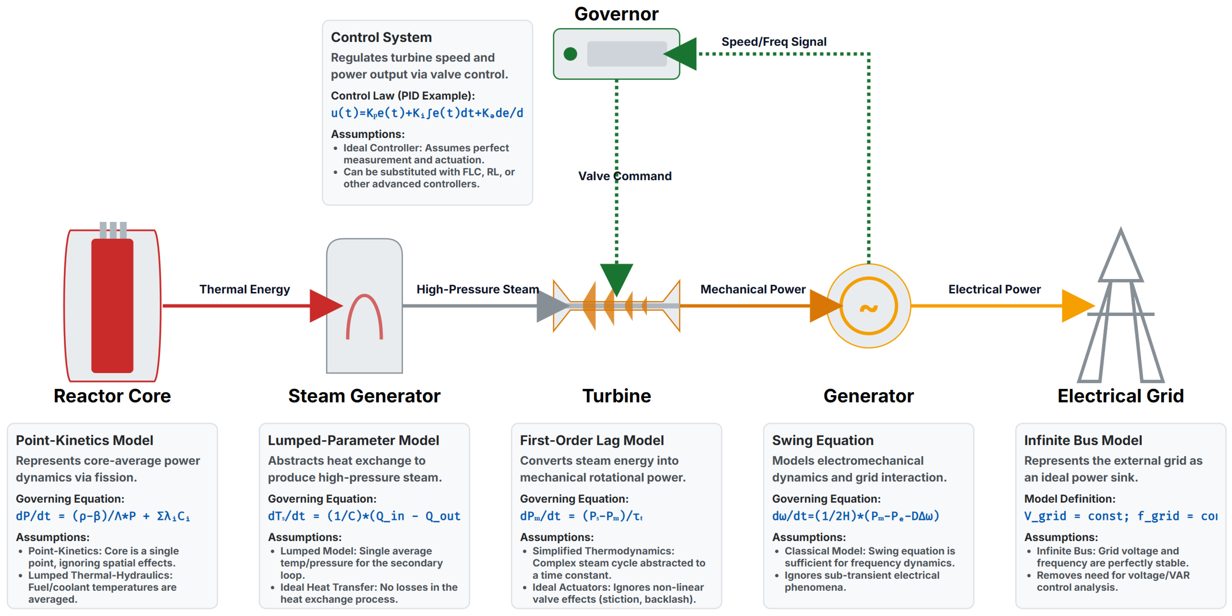
Figure 2 presents the schematic of the high-fidelity Pressurized Water Reactor (PWR) simulation model, which functions as the core testbed (Layer 3) within the DTAF. The model accurately captures the plant’s essential dual-loop thermodynamic processes critical for load-following simulations. The Primary Loop circulates pressurized water to transfer thermal energy from the Reactor Core to the Steam Generator. The Pressurizer maintains the high system pressure required to prevent the primary coolant from boiling. In the Secondary Loop, this thermal energy is converted into electrical power. Water in the Steam Generator boils, producing high-pressure steam that drives the turbine. The turbine’s rotational energy is converted into electricity by the generator, which is synchronized with the Electrical Grid. This diagram highlights the primary control interface for the AI agent. The agent’s scalar action output directly actuates the Governor Valve (A_v), which regulates the mass flow rate of steam to the turbine. The agent’s control objective is to modulate this valve to maintain the stability of the grid frequency (f) by balancing power generation with grid demand, particularly during challenging load-following transients.

Clarification on the Digital Model and Framework Scope:

It is important to clarify the precise role of the PWR simulation within the DTAF. In this study, the high-fidelity model serves as a digital model—a validated, self-contained simulation environment that acts as a representative proxy for the physical plant. While the term ‘digital twin’ often implies a persistent, bidirectional data link to a specific physical asset, our use here refers to a high-fidelity simulation testbed.

The primary novelty of this paper is the DTAF itself: a model-agnostic assurance workflow. The ‘bidirectional data exchange’ and ‘communication protocols’ are therefore software-in-the-loop (SIL) interactions, representing the data passed between the DTAF’s analysis engine and the simulation environment (i.e., states, actions, and rewards). The DTAF is architected to be equally applicable to a fully-fledged digital twin or even a physical system in a hardware-in-the-loop (HIL) configuration. This study uses the high-fidelity digital model to formally validate the framework’s ability to assess, stress-test, and certify controller behavior against established benchmarks. The DTAF framework can be extended in future work to a full-scale digital twin.

3.1.1. Neutron Point Kinetics (Six Delayed Groups)

$$\Lambda \ast \stackrel{.}{\mathrm{x}}n\left(t\right)=\left(\rho \left(t\right)-\beta \right)\ast n\left(t\right)+{\sum }_{i=1}^6{\lambda }_i\ast C_i\left(t\right)+S\left(t\right)$$

(1)

where n(t) is the normalized neutron density [-]; Λ is the prompt neutron generation time [s]; ρ_(t) is the total reactivity [Δk/k]; β is the total delayed neutron fraction [-]; ${\mathit{\lambda }}_{\mathit{i}}$ is the decay constant of precursor group i [s⁻¹]; $C_i\left(t\right)$ is the concentration of group-i precursors [-]; and S(t) is an external source (set to 0 in nominal runs).

$$\stackrel{.}{\mathrm{x}}{C}_i\left(t\right)=\left({\beta }_i/\Lambda \right)\ast n\left(t\right)-{\lambda }_i\ast C_i\left(t\right),i=1,\dots ,6$$

(2)

where β_i is the fraction of delayed neutrons from group i [-], satisfying ∑_{I = 1}^{6} β_i = β.

3.1.2. Reactivity Feedback and Power Mapping

$$\rho \left(t\right)={\rho }_{ext}\left(t\right)+{\alpha }_f\ast \left(T_f\left(t\right)-T_{f}0\right)+{\alpha }_c\ast \left(T_c\left(t\right)-T_{c}0\right)$$

(3)

where ρ_ext (t) is the exogenous reactivity [Δk/k] (0 in this study); ${\alpha }_f$, ${\alpha }_c$ are the fuel and coolant temperature coefficients [Δk/k*°C⁻¹]; $T_f\left(t\right)$ and T_c(t) are the lumped fuel and coolant temperatures [°C]; and $T_{f}0$ and $T_{c}0$ are the reference temperatures [°C]. Here ${\alpha }_f$ = 0 and ${\alpha }_c$ = 0 to isolate the controller behavior deterministically.

$$P_{th}\left(t\right)={\kappa }_P\ast n\left(t\right)$$

(4)

where $P_{th}$ (t) is the reactor thermal power [MW] and ${\kappa }_P$ = 1000.0 MW maps the normalized neutron density to thermal power.

3.1.3. Lumped Thermal–Hydraulic Model

$$C_f\ast \stackrel{.}{\mathrm{x}}{T}_f\left(t\right)=P_{th}\left(t\right)-U_{fc}\ast \left(T_f\left(t\right)-T_c\left(t\right)\right)$$

(5)

where $C_f$ = 30.0 MJ/°C is the effective fuel heat capacity and $U_{fc}$ = 2.0 MW/°C is the fuel-coolant conductance.

$$C_c\ast \stackrel{.}{\mathrm{x}}{T}_c\left(t\right)=U_{fc}\ast \left(T_f\left(t\right)-T_c\left(t\right)\right)-U_{cs}\ast \left(T_c\left(t\right)-T_{s0}\right)$$

(6)

where $C_c$ = 50.0 MJ/°C is the effective coolant heat capacity; $U_{cs}$ = 20.0 MW/°C is the coolant-secondary conductance; and $T_{s0}$ = 270.0 °C is the fixed secondary-side sink temperature.

3.1.4. Valve, Turbine-Governor, and Generator

$${\tau }_v\ast \stackrel{.}{\mathrm{x}}v\left(t\right)=u\left(t\right)-v\left(t\right),v\in \left[\mathrm{0,1}\right]$$

(7)

where v_(t) is the valve position [-]; u_(t) is the controller command [-]; and ${\tau }_v$ = 0.30 s is the valve-servo time constant. A deterministic rate limiter | $\stackrel{.}{\mathrm{x}}v$ | ≤ r_max with r_max = 0.15 s⁻¹ is applied to the commanded motion.

$${\tau }_m\ast \stackrel{.}{\mathrm{x}}{P}_m\left(t\right)=K_t\ast v\left(t\right)-P_m\left(t\right)$$

(8)

where $P_m\left(t\right)$ is the mechanical power into the turbine [MW]; ${\tau }_m$ = 3.0 s is the steam-path/turbine lag; and $K_t$ = 900.0 MW/- maps the valve to mechanical power.

$$P_e\left(t\right)={\eta }_g\ast P_m\left(t\right)$$

(9)

where $P_e\left(t\right)$ is the electrical power to the grid [MW] and ${\eta }_g$ = 0.98 is the generator efficiency.

3.1.5. Measured Outputs and Signals

$$y\left(t\right)={\left[P_e\left(t\right),v\left(t\right),T_f\left(t\right),T_c\left(t\right)\right]}^T,f\left(t\right)=f_{grid}\left(t\right),f_{nom}=60 \mathrm{H}\mathrm{z}$$

(10)

where y_(t) collects the outputs used by controllers and metrics; f_(t) is the measured grid frequency [Hz] from the infinite bus; and $f_{nom}$ = 60 Hz is nominal.

3.1.6. Parameters and Numerics

Numerical integration uses a fixed step Δt = 0.05 s (forward Euler). Initial conditions correspond to the steady-state at P_e = P_ref = 600 MW with infinite-bus synchronism. The implied nominal valve position is v₀ ≈ P_ref/(η_g * K_t) = 600/(0.98 * 900) ≈ 0.680, and the thermal states satisfy (5) and (6) at steady power with $T_{s}0$.

The six-group point-kinetics constants used in (1) and (2) are drawn from a standard PWR benchmark set, and can be seen in

Table 1. Neutron kinetics constants.

Symbol	Description	Value	Units
β	Total delayed neutron fraction	0.006502	-
Λ	Prompt neutron generation time	1.0 × 10−4	s
${\lambda }_1$	Precursor decay constant (group 1)	0.0124	s−1
${\lambda }_2$	Precursor decay constant (group 2)	0.0305	s−1
λ3	Precursor decay constant (group 3)	0.111	s−1
λ4	Precursor decay constant (group 4)	0.301	s−1
${\lambda }_5$	Precursor decay constant (group 5)	1.14	s−1
${\lambda }_6$	Precursor decay constant (group 6)	3.01	s−1

.

For reproducibility of the precursor balance in (2), the delayed-neutron fractions are provided per group, as seen in

Table 2. Delayed neutron fractions per group (six-group; sum to β).

Symbol	Description	Value	Units
${\beta }_1$	Group-1 delayed neutron fraction	0.000215	-
${\beta }_2$	Group-2 delayed neutron fraction	0.001424	-
${\beta }_3$	Group-3 delayed neutron fraction	0.001274	-
${\beta }_4$	Group-4 delayed neutron fraction	0.002568	-
${\beta }_5$	Group-5 delayed neutron fraction	0.000748	-
${\beta }_6$	Group-6 delayed neutron fraction	0.000273	-

Note: ${\beta }_1$ + ${\beta }_2$ + ${\beta }_3$ + ${\beta }_4$ + ${\beta }_5$ + ${\beta }_6$ = 0.006502 = β.

.

The thermal blocks used in (5) and (6) and the power-mapping in (4) use the constants listed below in

Table 3. Thermal–hydraulic and power-mapping constants.

Symbol	Description	Value	Units
κP	Power scaling (n → MW_th)	1000.0	MW
Cf	Effective fuel thermal capacity	30.0	MJ/°C
Cc	Effective coolant thermal capacity	50.0	MJ/°C
Ufc	Fuel-coolant conductance	2.0	MW/°C
Ucs	Coolant-secondary conductance	20.0	MW/°C
Ts0	Secondary-side sink temperature (fixed)	270.0	°C

.

The valve servo (7), turbine path (8), and electrical output (9) are parameterized as follows in

Table 4. Turbine-governor and grid constants.

Symbol	Description	Value	Units
τv	Valve servo time constant	0.30	s
τm	Steam-path/turbine lag	3.0	s
Kt	Turbine gain (v → P_m)	900.0	MW/-
ηg	Generator efficiency	0.98	-
fnom	Nominal grid frequency	60.0	Hz
Pref	Nominal electrical power reference	600.0	MW

.

Actuator bounds and the integration step used throughout are summarized next, as seen in

Table 5. Actuator limits and numerical step.

Symbol	Description	Value	Units
$u_{min}$	Valve lower bound	0.0	-
$u_{max}$	Valve upper bound	1.0	-
$r_{max}$	Valve rate limit	0.15	s−1
Δt	Numerical integration step	0.05	s

.

3.2. Controllers

3.2.1. Proportional–Integral–Derivative (PID) Governor

We employ a discrete-time PID with a filtered derivative and conditional anti-windup. Letting $e\left(k\right)$ = r(k) − $y\left(k\right)$ be the tracking error, Δt the loop period, $u\left(k\right)\in \left[u_{min},u_{max}\right]$ the valve command, and $r_{max}$ the rate limit, saturation precedes rate limiting.

$$u_P\left(k\right)=K_p\ast e\left(k\right)$$

(11)

where $K_p$ is the proportional gain [—], and e(k) is the tracking error (setpoint minus measured output).

$$I\left(k\right)=I\left(k-1\right)+K_i\ast \Delta t\ast e\left(k\right)$$

(12)

where $K_i$ is the integral gain [s⁻¹], and $\Delta t$ is the loop period [s].

$${\tau }_d\ast d\psi /dt+\psi \left(t\right)=de/dt,u_D\left(t\right)=K_d\ast \psi \left(t\right)$$

(13)

where ψ_(t) is the filtered derivative state [1/s]; τ_d is the derivative filter time constant [s]; and $K_d$ is the derivative gain [s].

$$\psi \left(k\right)=a\ast \psi \left(k-1\right)+b\ast \left(e\left(k\right)-e\left(k-1\right)\right),a=\left(2\ast {\tau }_d-\Delta t\right)/\left(2\ast {\tau }_d+\Delta t\right),b=2/\left(2\ast {\tau }_d+\Delta t\right)$$

(14)

where ψ_(k) is the discrete filtered derivative; and a and b are bilinear (Tustin) coefficients ensuring a stable first-order low-pass on the derivative of e_(k).

$$u_D\left(k\right)=K_d\ast \psi \left(k\right)$$

(15)

where $u_D\left(k\right)$ is the derivative contribution to the command [-].

$$u_{raw}\left(k\right)=u_P\left(k\right)+I\left(k\right)+u_D\left(k\right)$$

(16)

where $u_{raw}\left(k\right)$ is the unsaturated command [-].

$$u_{sat}\left(k\right)=min\left(max\left(u_{raw}\left(k\right),u_{min}\right),u_{max}\right)$$

(17)

enforcing the physical valve limits u_min ≤ u_sat(k) ≤ u_max.

$$u\left(k\right)=u\left(k-1\right)+clip\left(u_{sat}\left(k\right)-u\left(k-1\right),-r_{max}\ast \Delta t,r_{max}\ast \Delta t\right)$$

(18)

Post-saturation rate limiting ensures |u_(k) − u_{(k − 1)}| ≤ $r_{max}$·Δt.

The PID gains and limits used in all deterministic runs are fixed and listed below in

Table 6. PID parameters.

Symbol	Description	Value	Units
$K_p$	Proportional gain	1.800	-
$K_i$	Integral gain	0.300	s−1
Kd	Derivative gain	0.050	s
τd	Derivative filter time constant	0.200	s
$u_{min}$	Valve lower bound	0.0	-
$u_{max}$	Valve upper bound	1.0	-
$r_{max}$	Valve rate limit	0.15	s−1
Δt	Loop period (numerical step)	0.05	s

.

3.2.2. Mamdani Fuzzy-Logic Governor (FLC)

The FLC uses two antecedents—error e and error-rate $\Delta e$—and one consequent Δu. Each linguistic variable employs five triangular/trapezoidal sets {NB, NS, ZE, PS, PB}. Inputs are scaled by s_e and s_Δe; the consequent is scaled by s_u. Implication is min(·), aggregation is max(·), and defuzzification is the centroid.

$$e_s=e/s_e,\Delta e_s=\left(\Delta e\right)/s_{\Delta e}$$

(19)

where e_s and Δe_s are scaled antecedents [-]; s_e and s_{Δe} are their scales [-].

$${\mu }_{C_{ij}}\left(z\right)=min\left({\mu }_{A_i}\left(e_s\right),{\mu }_{B_j}\left(\Delta e_s\right)\right)$$

(20)

where R_{ij}: (A_i, B_j) → C_{ij} are the rules; implication uses min(·).

$${\mu }_C\left(z\right)=ma{x}_{i,j}{\mu }_{C_{ij}}\left(z\right)$$

(21)

where ${\mu }_C\left(z\right)$ is the aggregated consequent membership [—].

$$\Delta u=s_u\ast \left(\int z\ast {\mu }_C\left(z\right)dz\right)/\left(\int {\mu }_C\left(z\right)dz\right)$$

(22)

where s_u is the output scale [-]; Δu is the defuzzified valve increment [-]; and the final command u is obtained by accumulating Δu and enforcing (17) and (18).

$${\mu }_{TRI}\left(z;a,b,c\right)=max\left(min\left(\left(z-a\right)/\left(b-a\right),\left(c-z\right)/\left(c-b\right)\right),0\right)$$

(23)

is the normalized triangular membership function used for NB, NS, ZE, PS, PB with breakpoints (a ≤ b ≤ c) clamped to z ∈ [−1, 1].

The 5 × 5 rule base maps (e, Δe) to Δu linguistic labels as follows, in

Table 7. FLC rule base (rows: Δe; columns: e).

Δe\e	NB	NS	ZE	PS	PB
NB	PB	PB	PS	ZE	ZE
NS	PB	PS	ZE	NS	ZE
ZE	PS	ZE	ZE	ZE	NS
PS	ZE	NS	ZE	NS	NB
PB	ZE	ZE	NS	NB	NB

.

Input/output scales are fixed and listed next in

Table 8. FLC scaling parameters.

Symbol	Description	Value	Units
se	Error scaling	1.50	-
s{Δe}	Error-rate scaling	0.80	-
su	Output scaling	0.35	-

.

To ensure exact reproducibility of the FLC, normalized triangular membership breakpoints for e_s and Δe_s are provided in

Table 9. Normalized triangular MF breakpoints for antecedents (centers at −1, −0.5, 0, 0.5, and 1; ~50% overlap; clamped to [−1, 1]).

Label	a	b	c
NB	−1.00	−1.00	−0.50
NS	−1.00	−0.50	0.00
ZE	−0.50	0.00	0.50
PS	0.00	0.50	1.00
PB	0.50	1.00	1.00

.

3.2.3. Observation Normalization and Safety Bounds

Continuous variables are normalized by fixed scales ${\mathit{S}}_{\mathit{i}}$ and clipped to admissible bounds. Safety gates are deterministically applied and terminate an episode when violated.

$$x_{norm,i}=clip\left(x_i/S_i,x_{i,min},x_{i,max}\right)$$

(24)

where x{_norm,i} denotes the normalized i_th component. We avoid hat/overbar diacritics to guarantee robust rendering across Word installations.

The normalization scales and safety thresholds used in all runs are listed below in

Table 10. Normalization scales and safety thresholds (deterministic).

Symbol	Quantity	Value	Units	Notes
SP	Reactor power (scale)	1000.0	MW	Normalization divisor for P
ST	Fuel temperature (scale)	1000.0	°C	Normalization divisor for T_fuel
Sf	Grid frequency (scale)	1.0	Hz	Normalization divisor for f
Sω	Rotor speed (scale)	1.0	pu	Normalization divisor for ω
f{trip}	Under-frequency trip gate	49.00	Hz	Hard safety gate
$\left|\Delta f\right|calm$	Calm band (frequency)	0.02	Hz	Calm multiplier applies if ≤ value
$\left|\Delta P\right|calm$	Calm band (power)	2.0	MW	Calm multiplier applies if ≤ value

.

3.2.4. Reward Shaping

Reward is defined once here and referenced in downstream Section 3.3 and Section 3.4 without redefinition. A calm-state multiplier attenuates penalties inside tight frequency/power bands to reduce chattering.

$$r_t=-{\kappa }_t\ast \left[w_f\ast {\left(\Delta f_t\right)}^2+w_{move}\ast \left|\Delta u_t\right|+w_{jerk}\ast \left|\Delta u_t-\Delta u_{t-1}\right|\right]+b_t$$

(25)

where κ_t gates penalties during calm periods (Table 10). All weights are dimensionless because signals are normalized.

Reward weights and bonuses (dimensionless) are fixed as follows in

Table 11. Reward weights and bonuses (dimensionless).

Symbol	Description	Value	Units	Notes
wf	Frequency error penalty	1.00	-	Primary stability focus
w{move}	Valve movement penalty	0.010	-	Economy and wear proxy
w{jerk}	Valve jerk penalty	0.020	-	Penalizes reversals
w{bonus}	Safe completion bonus	5.00	-	Applied once if no gates breached
w{unsafe}	Unsafe penalty	10.00	-	Applied on any gate violation
c{calm}	Calm-state multiplier	0.50	-	If |Δf| ≤ 0.02 Hz and |ΔP| ≤ 2 MW

.

3.2.5. Five-Phase Curriculum

Training progresses through five deterministic phases. Advancement requires zero safety breaches across the current phase’s evaluation bundle and non-decreasing mean reward.

$$N_{unsafe}=0\wedge r_{avg}^{\left(k\right)}\ge r_{avg}^{\left(k-1\right)}$$

(26)

where N_{unsafe} is the count of safety-gate violations in the phase evaluation bundle and r_{avg}^{(k)} is the mean return for phase k. The wedge symbol ∧ expresses logical AND and avoids ‘0AND’ concatenation issues.

Curriculum phases, scenario bundles, and promotion conditions are summarized below in

Table 12. Deterministic curriculum phases and promotion conditions.

Symbol	Phase	Scenario Bundle	Promotion Threshold	Reward Overrides
P1	Stability and limits	Baseline; ramp-in-place	Nunsafe = 0; non-decreasing ravg	Increasing ↑ wf; enable calm multiplier
P2	Efficiency	Baseline; gradual load	Nunsafe = 0; non-decreasing ravg	Increasing ↑ wmove
P3	Disturbances I	Sensor-noise; parameter ramp (deterministic)	Nunsafe _{unsafe} = 0; non-decreasing ravg	Increasing ↑ wjerk
P4	Disturbances II	Cascading-fault	Nunsafe = 0; non-decreasing ravg	Keep P2/P3 overrides
P5	Final exam	Combined	Nunsafe = 0; non-decreasing ravg	Freeze weights; evaluate only

Where “↑” denotes a metric to be maximized (higher values are better).

.

3.2.6. Soft Actor–Critic (SAC) Governor

We use a tanh-squashed Gaussian policy with twin Q-critics and target networks. During evaluation, the action is mapped to the valve command and constrained by the same saturation and rate-limit logic in (17) and (18).

$$a=tanh\left({\mu }_{\theta }\left(s\right)+{\sigma }_{\theta }\left(s\right)\odot \epsilon \right),\epsilon ~N\left(0,I\right)$$

(27)

where ⊙ denotes the elementwise product between ${\sigma }_{\theta }\left(s\right)$ and $\epsilon$, with ε drawn from a standard normal.

$$log{\pi }_{\theta }\left(a|s\right)=logN\left(z;{\mu }_{\theta },{\sigma }_{\theta }\right)-{\sum }_{i}log\left(1-tanh{\left(z_i\right)}^2\right),z=artanh\left(a\right)$$

(28)

$$y=r+\left(1-d\right)\ast \gamma \ast \left(mi{n}_j{Q}_j^{targ}\left(s^{’},a^{’}\right)-\alpha \ast log{\pi }_{\theta }\left(a^{’}|s^{’}\right)\right),a^{’}~{\pi }_{\theta }\left(·|s^{’}\right)$$

(29)

$$L_Q=E\left[{\left(Q_i\left(s,a\right)-y\right)}^2\right],i\in \mathrm{1,2}$$

(30)

$$L_{\pi }=E\left[\alpha \ast log{\pi }_{\theta }\left(a|s\right)-mi{n}_i{Q}_i\left(s,a\right)\right]$$

(31)

$$L_{\alpha }=E\left[-\alpha \ast \left(log{\pi }_{\theta }\left(a|s\right)+H\ast \right)\right]$$

(32)

$${\phi }^{targ}\leftarrow \tau \ast \phi +\left(1-\tau \right)\ast {\phi }^{targ}$$

(33)

where $\phi$ are the critic parameters and ${\phi }^{targ}$ are the target-critic parameters updated by Polyak averaging with rate τ.

The SAC hyperparameters used in this work are listed below in

Table 13. SAC hyperparameters (values used).

Symbol	Name	Value	Units	Notes
α	Entropy temperature	auto-tuned	-	Target entropy heuristic
γ	Discount factor	0.99	-	Stable defaults
τ	Polyak rate	0.005	-	Target critic averaging
ηQ	Critic learning rate	3 × 10−4	-	Adam
ηπ	Actor learning rate	3 × 10−4	-	Adam
ηα	Temperature learning rate	3 × 10−4	-	If α learnable
B	Batch size	1024	samples	Minibatch size
|D|	Replay capacity	1,200,000	transitions	FIFO
N0	Learning starts	120,000	steps	Warm-up
T	Total timesteps	15,000,000	steps	Training budget
feval	Evaluation frequency	80,000	steps	Deterministic evals
policy	Policy/widths	MlpPolicy/[512,512]	-	Hidden units

.

Replay/evaluation cadence is deterministic and fixed as follows in

Table 14. Replay/batch schedule and evaluation settings.

Symbol	Quantity	Value	Units	Notes
tstep	Environment step time	Δt	s	Loop period from plant interface
Nupdate	Updates per env step	1	-	Once learning starts
Ntarget	Target update cadence	1	-	Per gradient step
evaldet	Deterministic evaluation	enabled	-	No exploration noise

.

3.2.7. Differential Evolution (DE) for Deterministic Tuning

We tune PID { K_p, K_i, K_d, τ_d } and FLC { s_e, s_Δe, s_u } using SciPy’s DE (strategy = ‘best1bin’) on a fixed catalogue of scenarios. The objective aggregates metrics to minimize (M↓) and to maximize (M↑), with a failure penalty per gate violation.

$$J\left(\theta \right)={\sum }_{m\in M\downarrow }{w}_{m}m\left(\theta \right)-{\sum }_{h\in M\uparrow }{w}_{h}h\left(\theta \right)+\lambda N_{fail}\left(\theta \right)$$

(34)

The metric weights used in the DE objective are listed below in

Table 15. Metric weights used in J(θ).

Symbol	Metric	Group	Weight	Notes
wTSS	Transient Severity Score (TSS)	M ↓	1.00	Primary stability objective
wCE	Cumulative actuation effort (CEsum)	M ↓	0.50	Economy objective
wVrev	Valve reversals (Vrev)	M ↓	0.50	Mechanical wear proxy
wGLFI	Grid Load-Following Index (GLFI)	M ↑	1.00	Tracking quality
λ	Failure penalty multiplier	100	—	Scaled by Nfail (θ)

Note: “↓” denotes a metric to be minimized (lower values are better); “↑” denotes a metric to be maximized (higher values are better).

.

The bounds and algorithmic settings for DE are shown next in

Table 16. DE bounds and algorithm parameters.

Symbol	Parameter	Bounds/Value	Units	Notes
Kp	PID proportional gain	[0.5, 3.0]	-	Search bound
Ki	PID integral gain	[0.05, 0.8]	s−1	Search bound
Kd	PID derivative gain	[0.00, 0.15]	s	Search bound
τd	Derivative time constant	[0.05, 0.50]	s	Search bound
se	FLC error scale	[0.5, 2.5]	-	Search bound
sΔe	FLC error-rate scale	[0.3, 1.5]	-	Search bound
su	FLC output scale	[0.1, 0.8]	-	Search bound
F	DE mutation scale	[0.5, 1.0]	-	Differential weight
Cr	DE crossover probability	0.7	-	Crossover rate
Gmax	Max iterations	50 (PID)/30 (FLC)	generations	Stopping criterion
P	Population size	15	candidates	Per generation
tol	Convergence tolerance	1 × 10−2	-	Early stop threshold

and Algorithm 1 as following:.

Algorithm 1. DE-based multi-scenario tuning.
0	procedure DA_LGE(DT, C = {PID_DE, FLC_DE, SAC}, S, K, G, primary_seed)
1	▷ Inputs: digital twin DT(Δt), controllers C, scenario portfolio S,
1a	KPI set K, licensing gates G, primary_seed
2	▷ Outputs: ranking, PASS_c, CRS_c per controller, portfolio report, evidence bundle
3	set_random_seed(primary_seed); enable_global_determinism()
4	for each controller c in C do
5	if c ∈ {PID_DE, FLC_DE} then
6	θ_c ← DifferentialEvolution(J_multi_scenario, bounds, seed = primary_seed)
7	freeze(θ_c)
8	end if
9	R_c ← ∅ ▷ portfolio record for controller c
10	for each scenario s in S do
11	reset(DT, initial_state = s.x0, power_level = s.P)
12	schedule_disturbances(DT, s.disturbances)    ▷ deterministic
13	for k = 0 … ⌊s.T/Δt⌋ − 1 do
14	y_k ← sense(DT)
15	u_k ← policy_c(y_k)
16	u_k ← rate_limit(saturate(u_k))
17	x_{k + 1} ← step(DT, u_k, Δt)
18	log⟨k, x_k, y_k, u_k⟩
19	end for
20	m_{c,s} ← compute_KPIs(K, log)
21	g_{c,s} ← evaluate_gates(G, m_{c,s})    ▷ vector of PASS/FAIL
22	r_{c,s} ← composite_score(m_{c,s}, g_{c,s})
23	R_c ← R_c ∪ {(s, m_{c,s}, g_{c,s}, r_{c,s})}
24	end for
25	CRS_c ← aggregate_scores({r_{c,s}}_s; weights = s.weights)
26	PASS_c ← all_gates_pass({g_{c,s}}_s; hard_fail = ‘any’)
27	end for
28	ranking ← sort_by((PASS_c ↓, CRS_c ↓, var({r_{c,s}}) ↑))
29	export_evidence({R_c}_c, configs, seeds, figures, tables)
30	return ranking, {PASS_c, CRS_c}_c, {R_c}_c
31	end procedure
Legend: Δt—simulation step; DE—Differential Evolution; KPIs—tracking/overshoot/settling/unsafe time/control effort; G—licensing gates (hard); CRS—composite rating score; PASS_c—portfolio pass if any hard gate fails → FAIL. Note: PID_DE: Differenfial Evolution opitimized PID, FLC_DE: Differenfial Evolution opitimizedFLC.

3.2.8. Evidence Capture and Reproducibility

All runs emit versioned logs, checkpoints, and manifests. The following artifacts are produced deterministically at the paths shown.

The artifacts generated by the pipeline are summarized below in

Table 17. Evidence artifacts emitted by the pipeline.

Symbol	Artifact	Path/Identifier	Frequency	Mechanism
A1	Raw evaluation logs	results/logs/*.csv	Per eval	Auto-export
A2	Training checkpoints	results/checkpoints/*.zip	Per save step	SB3 saver
A3	Best model	results/best/*.zip	On improvement	Eval callback
A4	Final model	results/final/*.zip	End of training	Export final
A5	Reports/figures	results/reports/*	On demand	Figure scripts
A6	Config manifests	results/config/*.yml	Per run	Hash-locked

Note: “*” denotes a wildcard matching multiple files in the specified directory (e.g., results/logs/run1.csv).

.

3.3. Evaluation Scenarios—Deterministic Disturbance Models, Execution Protocol, and Metrics

This subsection defines the deterministic scenario catalogue, the disturbance models applied to the plant–grid interface, the execution protocol used to evaluate each controller, and the metric suite collected per scenario.

We first define two helper operators used throughout: the clipping operator in (35) and the time-window indicator in (36).

$$clip\left(x;a,b\right)=min\left(max\left(x,a\right),b\right)$$

(35)

where clip(x; a, b) saturates a scalar x to the closed interval [a, b].

$$w_{\left[a,b\right]}\left(t\right)=1,a\le t\le b;0,otherwise$$

(36)

where $w_{\left[a,b\right]}\left(t\right)$ is a deterministic 0–1 window that activates a disturbance on the interval [a, b] (seconds).

3.3.1. Deterministic Scenario Catalogue and Disturbance Models

Letting ${\mathit{P}}_{\mathit{r}\mathit{e}\mathit{f}}$ denote the nominal electrical load (MW), and ΔL_ref a reference load change magnitude (MW), the commanded load profile L(t) for each scenario is defined below.

Baseline steady operation holds a constant demand level, as in (37).

$$L_{base}\left(t\right)=P_{ref}$$

(37)

where $L_{base}\left(t\right)$ is the baseline demand (MW) and ${\mathit{P}}_{\mathit{r}\mathit{e}\mathit{f}}$ is the nominal power setpoint (MW).

A gradual load increase is modeled as a linear ramp over [t₁, t₂], clipped outside the interval, as in (38).

$$L_{grad}\left(t\right)=P_{ref}+\Delta L_{ref}\ast clip\left(\left(t-t_1\right)/\left(t_2-t_1\right);\mathrm{0,1}\right)$$

(38)

where 0 ≤ (t – t₁)/(t₂− t_1) ≤ 1 over the ramp, and ΔL_{ref} > 0 (MW).

A sudden load increase is represented by a deterministic step at time $t_s$ in (39).

$$L_{step}\left(t\right)=P_{ref}+\Delta L_{ref}\ast w_{\left[t_s,T\right]}\left(t\right)$$

(39)

where T is the evaluation horizon (s) and ${\mathit{w}}_{\left[{\mathit{t}}_{\mathit{s}},\mathit{T}\right]}\left(\mathit{t}\right)$ activates the step at t = $t_s$.

Sensor-noise injection is deterministic and bounded: fixed multi-tone sinusoids are superposed on measured channels, as in (40) and (41).

$$n_f\left(t\right)=A_{f,1}sin\left(2\pi f_{1}t\right)+A_{f,2}sin\left(2\pi f_{2}t+{\phi }_2\right)$$

(40)

$$f_m\left(t\right)=f\left(t\right)+n_f\left(t\right),P_m\left(t\right)=P\left(t\right)+n_P\left(t\right)$$

(41)

where $f\left(t\right)$ is the true grid frequency (Hz), P(t) is the plant electrical power (MW), $f_m\left(t\right)$ and $P_m$ are their measured counterparts, $n_f\left(t\right)$ and $n_P\left(t\right)$ are deterministic noise signals, and $A_{f,1}$, $A_{f,2}$, $f_1$, $f_2$, and ${\phi }_2$ are fixed constants provided in

Table 18. Scenario parameters (deterministic values).

Symbol	Description	Value	Units
T	Evaluation horizon	600	s
Δt	Controller/eval step	0.05	s
fnom	Nominal grid frequency	60.0	Hz
$\Delta L_{ref}$	Reference load change magnitude	0.04·P_{ref}	MW
t1, t2	Gradual ramp window	120, 300	s
ts(s)	Sudden step time	60	s
$t_a,t_b$	Fault window #1	120, 210	s
$t_c,t_d$	Fault window #2	360, 420	s
$A_{f,1}$, $A_{f,2}$	Frequency-noise amplitudes	0.003, 0.002	Hz
$f_1,f_2$	Noise tones (frequency)	0.6, 1.2	Hz
Φ2	Noise phase	1.0472	rad (≈60°)

.

Parameter-ramp disturbances alter selected plant parameters deterministically over a window, as in (42).

$${\theta }_i\left(t\right)={\theta }_{i,0}+r_i\ast \left(t-t_1\right)\ast w_{\left[t_1,t_2\right]}\left(t\right)$$

(42)

where ${\theta }_i\left(t\right)$ is the nominal value of parameter i, $r_i$ is the ramp rate (units of ${\theta }_i$ per second), and ${\mathit{w}}_{\left[{\mathit{t}}_1,{\mathit{t}}_2\right]}\left(\mathit{t}\right)$ gates the change.

A cascading-fault profile is defined by sequential windows on the load channel, as in (43).

$$L_{cf}\left(t\right)=P_{ref}+{\Delta }_1\ast w_{\left[t_a,t_b\right]}\left(t\right)-{\Delta }_2\ast w_{\left[t_c,t_d\right]}\left(t\right)$$

(43)

where ${\Delta }_1$, ${\Delta }_2$ > 0 (MW) and $\left[t_a,t_b\right]$, $\left[t_c,t_d\right]$ are non-overlapping windows that realize compounding stresses.

The combined scenario aggregates the foregoing signals in (44).

$$L_{comb}\left(t\right)=L_{base}\left(t\right)+{\Sigma }_q\Delta L_q\left(t\right)$$

(44)

where $\Delta L_q\left(t\right)$ denotes each active disturbance component (ramp, step, noise, parameter ramp, and fault) defined above.

Numerical values used in the deterministic disturbance models are fixed for all evaluations, as seen in Table 18.

3.3.2. Deterministic Execution Protocol

All controllers are evaluated with a single deterministic pass per scenario. For each scenario s, the environment is reset, the disturbance model L^s(t)is applied, safety gates are enforced, and the metric set is computed from the resulting closed-loop trajectory. The guard conditions and logging are deterministic and reproducible.

Evaluation proceeds as follows (high-level outline):

(1) Select a scenario (s) from the fixed catalogue; (2) reset state; (3) simulate for T seconds at step Δt under the deterministic disturbance; (4) enforce safety gates (frequency trip $f_{trip}$, thermal and speed limits) during rollout; (5) compute and store all metrics defined in Section 3.3.3; and (6) persist logs and traces.

Safety limits and constants referenced by the protocol are listed here for completeness, as seen in

Table 19. Safety gates and constants (deterministic).

Symbol	Description	Value	Units
$f_{trip}$	Under-frequency trip threshold	49.00	Hz
${\omega }_{max,limit}$	Max rotor speed (per-unit)	1.10	pu
$T_{fuel}^{max}$	Fuel temperature limit	1500	°C

.

3.3.3. Metrics Collected per Scenario

Letting f(t) be the grid frequency (Hz), $e_f\left(t\right)$ = f(t) − f_{nom} the frequency error, $u_k$ the valve command at discrete step k (per-unit), and N = T/Δt the number of samples, we define the metrics below; each equation is followed by the symbol explanations and units.

The frequency error is defined in (45), and the integral metrics $IS{E}_f$ and $IA{E}_f$ follow in (46) and (47).

$$e_f\left(t\right)=f\left(t\right)-f_{nom}$$

(45)

where $e_f\left(t\right)$ (Hz) is the frequency deviation from the nominal $f_{nom}$ (Hz).

$$IS{E}_f={\int }_0^T{\left(e_f\left(t\right)\right)}^{2}dt$$

(46)

where $IS{E}_f$ has units Hz²·s and aggregates the squared frequency error over the horizon [0, T].

$$IA{E}_f={\int }_0^T\left|e_f\left(t\right)\right|dt$$

(47)

where $IA{E}_f$ has units Hz·s and aggregates the absolute frequency error over [0, T].

The peak deviation and nadir are defined via extremum operators in (48).

$$\Delta f_{max}=ma{x}_{t\in \left[0,T\right]}\left|e_f\left(t\right)\right|,f_{nadir}=mi{n}_{t\in \left[0,T\right]}f\left(t\right)$$

(48)

where $\Delta f_{max}$ (Hz) is the largest magnitude deviation and $f_{nadir}$ (Hz) is the minimum frequency attained.

Rotor-speed overshoot and undershoot (percent) relative to nominal are defined in (49).

$$O{S}_{\omega }=100\%·ma{x}_t{\left(\omega \left(t\right)-1\right)}_{+},U{S}_{\omega }=100\%·ma{x}_t{\left(1-\omega \left(t\right)\right)}_{+}$$

(49)

where ω(t) is the rotor speed in per-unit, and (x)_{+} = max(x, 0) denotes the positive-part operator.

Cumulative actuation effort and valve reversals are computed from the discrete control sequence in (50) and (51).

$$C{E}_{sum}={\Sigma }_{k=1}^N\left|\Delta u_k\right|,\Delta u_k=u_k-u_{k-1}$$

(50)

where $C{E}_{sum}$ (dimensionless) accumulates the absolute valve movements (per-unit commands).

$$V_{rev}={\Sigma }_{k=2}^{N}1\left(\Delta u_k\right)\left(\Delta u_{k-1}\right)<0$$

(51)

where ${\mathit{V}}_{\mathit{r}\mathit{e}\mathit{v}}$ (count) is the number of sign reversals in the valve-movement sequence, and 1{·} is the indicator function.

Spectral damping is assessed from the Welch PSD ${\mathit{S}}_{\mathit{f}}\mathit{f}\left(\mathit{\omega }\right)$ of ${\mathit{e}}_{\mathit{f}}\left(\mathit{t}\right)$; the band-averaged magnitude is given in (52) and (53).

$$S_{f}f\left(\omega \right)=Welch{ e}_f\left(t\right)$$

(52)

where Welch{·} denotes a deterministic PSD estimate (fixed window/overlap).

$$E_{damp}=1/\left({\omega }_2-{\omega }_1\right)\ast {\int }_{{\omega }_1}^{{\omega }_2}{S}_{f}f\left(\omega \right)d\omega$$

(53)

where [${\mathit{\omega }}_2,{\mathit{\omega }}_1$] is the evaluation band (rad/s).

The total unsafe time, used later in licensing gates, is the sum of dwell times in any violating condition, as in (54).

$$T_{unsafe}=T\left(T_{fuel}>T_{fuel}^{max}\right)+T\left(\omega >{\omega }_{max,limit}\right)+T\left(f\notin \left[f_{min},f_{max}\right]\right)$$

(54)

where T(·) counts the time (s) spent in the indicated set, ${\mathit{\omega }}_{\mathit{m}\mathit{a}\mathit{x},\mathit{l}\mathit{i}\mathit{m}\mathit{i}\mathit{t}}$ is the rotor-speed limit (per-unit), and $\left[{\mathit{f}}_{\mathit{m}\mathit{i}\mathit{n}},{\mathit{f}}_{\mathit{m}\mathit{a}\mathit{x}}\right]$ is the accepted frequency band (Hz).

The Grid Load-Following Index (GLFI) is a bounded tracking score (higher is better), defined in discrete form in (55).

$$GLFI=1-\left(1/N\right)\ast {\Sigma }_{k=1}^N\left(\left|P_{e,k}-L_k\right|\right)/\left(\Delta L_{ref}+{\epsilon }_P\right)$$

(55)

where $P_{e,k}$ is the electrical power (MW) at sample k, $L_k$ is the commanded load (MW), $\Delta L_{ref}$ is the reference load change magnitude (MW), and ${\epsilon }_P$ = 1.0 MW is a physical denominator floor.

A composite Transient Severity Score (TSS) is formed as a weighted sum of normalized components in (56) and (57).

$$\widehat{CE}=C{E}_{sum}/C{E}_{abs,max}, \widehat{{\tilde{V}}_{rev}}=V_{rev}/V_{rev,max}$$

(56)

where $\mathit{C}{\mathit{E}}_{\mathit{a}\mathit{b}\mathit{s},\mathit{m}\mathit{a}\mathit{x}}$ = r_{max} · T provides a conservative bound on cumulative movement (dimensionless) and $V_{rev,max}$ = N − 2 bounds reversal counts (both constants listed in

Table 20. Metric normalization constants (fixed).

Symbol	Description	Value	Units	Derivation
rmax	Valve rate limit	0.15	s−1	From Section 3.2 PID/limits
T	Evaluation horizon	600	s	Scenario constant
N	Samples per episode	12,000	-	T/Δt with Δt = 0.05 s
${CE}_{abs,max}$	Max cumulative movement	90	-	$r_{max}$·T
$V_{rev,max}$	Max valve reversals	11,998	count	N − 2
${\epsilon }_P$	GLFI denominator floor	1.0	MW	Physical floor
ω1, ω2	PSD band (rad/s)	3.14, 12.57	rad/s	0.5–2.0 Hz

).

$$TSS=w_f·\left(IA{E}_f/IA{E}_{f,lim}\right)+w_{ce}· \widehat{CE}+w_{vr}· \widehat{{\tilde{V}}_{rev}}+w_{os}·\left(O{S}_{\omega }/O{S}_{\omega ,max}\right)$$

(57)

where all weights are dimensionless and satisfy $w_f$ + $w_{ce}$ + $w_{vr}$ + $w_{os}$ = 1; $IA{E}_{f,lim}$ (Hz·s) and $O{S}_{\omega ,max}$ (%) are scenario-family limits used for normalization.

The fixed constants used by the metric normalizations are listed here in Table 20.

Default metric weights used for the composite TSS are shown below; all are dimensionless, as seen in

Table 21. TSS weights and limits (dimensionless).

Symbol	Description	Value	Units
$w_f$	Frequency-error weight	0.50	-
wce	Control-effort weight	0.20	-
$w_{vr}$	Valve-reversal weight	0.20	-
$w_{os}$	Overshoot weight	0.10	-
$IA{E}_{f,lim}$	IAE_f normalization	60	Hz·s
$O{S}_{\omega ,max}$	Overshoot limit	5	%

.

3.4. Deterministic Assurance Orchestration and Evidence Pipeline

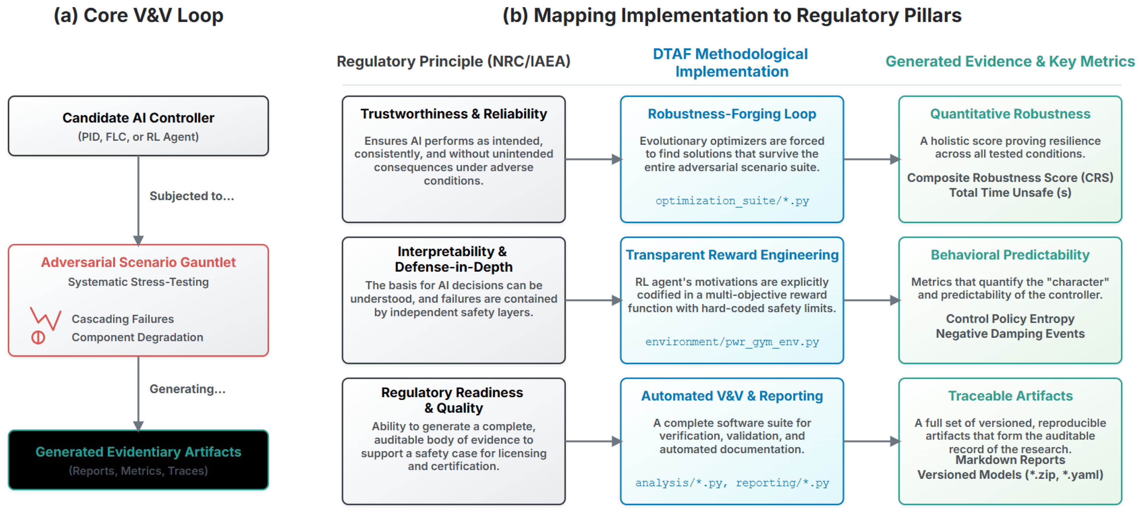
This subsection formalizes the Deterministic Assurance Framework used to qualify grid-interactive nuclear controllers. The framework binds scenario-level stress testing (Section 3.3), quantitative indicators, and evidence packaging into a single licensable pipeline. It is organized around four pillars—Trustworthiness and Reliability, Interpretability and Defense-in-Depth, Regulatory Readiness and Quality, and Continual Assurance—and produces auditable artifacts and objective pass/fail gates aligned to nuclear software and AI guidance (e.g., IAEA SSR-2/1 Criterion 5, NRC RG 1.168, NUREG-2261 Section 3.2, IEC 60880 [25] Category A). All evaluations are deterministic: scenarios S1–S8 are executed exactly as defined in Section 3.3, and the RL policy is evaluated with deterministic action selection. As shown in Figure 3, the Digital Twin Assurance Framework (DTAF) operationalizes these pillars by mapping stress-test evidence to licensable, regulator-aligned checks.

3.4.1. Control-Effort Indices and Hard Bounds

We first state the sample count used by all discrete-time metrics, and then derive hard bounds for cumulative movement and reversal counts.

$$N=T / \Delta t$$

(58)

where N is the number of samples per evaluation episode (—), T is the evaluation horizon (s), and Δt is the controller step size (s).

$$C{E}_{abs,max}=r_{max}\cdot T$$

(59)

where $C{E}_{abs,max}$ (—) is a conservative upper bound on cumulative valve movement, $r_{max}$ is the rate limit (s⁻¹), and T is the horizon (s). For $r_{max}$ = 0.15 s⁻¹ and T = 600 s, $C{E}_{abs,max}$ = 90.

$$V_{rev,max}=N-2$$

(60)

where $V_{rev,max}$ (count) is the maximum possible number of sign reversals in a sequence of length N (two samples are needed before a reversal can occur). With N = 12,000 (Δt = 0.05 s, T = 600 s), ${\mathit{V}}_{\mathit{r}\mathit{e}\mathit{v},\mathit{m}\mathit{a}\mathit{x}}$ = 11,998.

The weights used later in the composite robustness score (CRS) and the limits used by licensing gates are constants for all runs, as seen in

Table 22. CRS weights and licensing thresholds (dimensionless unless noted).

Symbol	Description	Value	Units/Notes
w safe	Safety contribution in CRS	0.40	-
w tss _{tss}	Transient severity contribution in CRS	0.30	-
w eff	Control-effort contribution in CRS	0.15	-
w glfi	Tracking contribution in CRS	0.15	-
$GLF{I}_{min}\hspace{0.25em}$	Minimum acceptable GLFI	0.90	-
$TS{S}_{lim}$	Upper bound on TSS	1.00	-
$O{S}_{\omega ,max}$	Max rotor-speed overshoot	5	%

.

3.4.2. Composite Robustness Score (CRS)

For each scenario s, a composite score $\mathit{C}\mathit{R}{\mathit{S}}^{\left(\mathit{s}\right)}$ is computed from the safety, transient severity, control effort, and tracking components. Safety contributes 1 when no unsafe dwell occurs and 0 otherwise; the other terms are normalized to [0, 1] (Section 3.3).

$$S^{\left(s\right)}=1\{\hspace{0.17em}{T}_{unsafe}^{\left(s\right)}=0\hspace{0.17em}\}$$

(61)

where S^s (—) is the per-scenario safety indicator, $\mathbb{1}${·} is the indicator function, and ${\mathit{T}}_{\mathit{u}\mathit{n}\mathit{s}\mathit{a}\mathit{f}\mathit{e}}^{\left(\mathit{s}\right)}$ is the total unsafe time in scenario (s)

$$CR{S}^{\left(s\right)}=w_{safe}{S}^{\left(s\right)}+w_{tss}\backslash big\left(1-TS{S}^{\left(s\right)}/TS{S}_{lim}\backslash big\right)+w_{eff}\backslash big\left(1-\widehat{C{E}^{\left(s\right)}\backslash }big\right)+w_{glfi}\cdot GLF{I}^{\left(s\right)}$$

(62)

where $\widehat{C{E}^{\left(s\right)}}$ = $\mathit{C}{\mathit{E}}_{\mathit{s}\mathit{u}\mathit{m}}$^{(s)}/$C{E}_{abs,max}$ (—) is the normalized control effort, $\mathit{G}\mathit{L}\mathit{F}{\mathit{I}}^{\left(\mathit{s}\right)}$ (—) is the tracking index, and $\mathit{T}\mathit{S}{\mathit{S}}^{\left(\mathit{s}\right)}$ (—) is the composite transient severity. Weights ${\mathit{w}}_{\mathit{s}\mathit{a}\mathit{f}\mathit{e}}$, ${\mathit{w}}_{\mathit{t}\mathit{s}\mathit{s}}$, ${\mathit{w}}_{\mathit{e}\mathit{f}\mathit{f}}$, and ${\mathit{w}}_{\mathit{g}\mathit{l}\mathit{f}\mathit{i}}$ are listed in Table 22.

3.4.3. Per-Scenario Licensing Gates

Per-scenario licensing gates combine deterministic constraints on safety, severity, tracking, and overshoot. Letting TTU ≡ $T_{unsafe}^{\left(s\right)}$, the logical gate is given in (63) and must evaluate to 1 for the scenario to qualify.

$$Gat{e}^{\left(s\right)}=1\{\hspace{0.17em}{T}_{unsafe}^{\left(s\right)}=0\hspace{0.25em}\wedge \hspace{0.25em}TS{S}^{\left(s\right)}\le TS{S}_{lim}\hspace{0.25em}\wedge \hspace{0.25em}GLF{I}^{\left(s\right)}\ge GLF{I}_{min}\hspace{0.25em}\wedge \hspace{0.25em}O{S}_{\mathsf{\omega }}^{\left(s\right)}\le O{S}_{\mathsf{\omega },max}\hspace{0.17em}\}$$

(63)

where ∧ denotes logical AND, $\mathit{T}\mathit{S}{\mathit{S}}_{\mathit{l}\mathit{i}\mathit{m}}$, $\mathit{G}\mathit{L}\mathit{F}{\mathit{I}}_{\mathit{m}\mathit{i}\mathit{n}}\hspace{0.25em}$, and $\mathit{O}{\mathit{S}}_{\mathsf{\omega },\mathit{m}\mathit{a}\mathit{x}}$ are constants from Table 22, and all quantities are computed deterministically from the rollout.

3.4.4. Policy Interpretability Constraint (Entropy Band)

To guard against both saturated and erratic policies, we bound the average action entropy $\overline{{\mathit{H}}_{\mathit{p}\mathit{r}\mathit{o}\mathit{x}\mathit{y}}}$ within a fixed band (nats), as shown in (64). Entropy is computed deterministically from the deployed policy’s squashed Gaussian outputs with a fixed sampling grid.

$$\overline{H_{proxy}}\in \left[H_{min},H_{max}\right]$$

(64)

where H_{min} and H_{{max} ()} define the acceptable interpretability band.

The entropy band used by the interpretability constraint is fixed for all evaluations, seen in

Table 23. Entropy band constants.

Symbol	Description	Value	Units
H{min}	Lower entropy bound	0.10	nats
H{max}	Upper entropy bound	2.00	nats

.

3.4.5. Portfolio Aggregation and Licensing Decision

Letting S be the number of scenarios in the catalogue (Section 3.3), we aggregate CRS across scenarios by the arithmetic mean and track the worst and best individual outcomes, as in (65). The final licensing decision is a deterministic logical gate (66) that combines the mean score, per-scenario gates, and the entropy band.

$$\overline{CRS}={\displaystyle \frac{1}{S}}{\sum }_{s=1}^{S}CR{S}^{\left(s\right)},\hspace{1em}CR{S}_{worst}=\underset{s}{\min }CR{S}^{\left(s\right)},\hspace{1em}CR{S}_{best}=\underset{s}{\max }CR{S}^{\left(s\right)}$$

(65)

$$Gat{e}_{portfolio}=1\{\hspace{0.17em}\overline{CRS}\ge CR{S}_{min}\hspace{0.25em}\wedge \hspace{0.25em}\mathrm{G}at{e}^{\left(s\right)}=1\hspace{0.25em}\wedge \hspace{0.25em}\overline{H_{proxy}}\in \left[H_{min},H_{max}\right]\hspace{0.17em}\}$$

(66)

where $\mathit{C}\mathit{R}{\mathit{S}}_{\mathit{m}\mathit{i}\mathit{n}}$ is the minimum acceptable mean CRS (—), $\mathit{G}\mathit{a}\mathit{t}{\mathit{e}}^{\left(\mathit{s}\right)}$ is the per-scenario gate from (63), and $\overline{{\mathit{H}}_{\mathit{p}\mathit{r}\mathit{o}\mathit{x}\mathit{y}}}$ is constrained by (64).

The portfolio-level constants are shown below and apply uniformly to all controllers evaluated under this framework, seen in

Table 24. Portfolio constants (dimensionless unless noted).

Symbol	Description	Value	Units
S	Number of scenarios	8	-
$\mathit{C}\mathit{R}{\mathit{S}}_{\mathit{m}\mathit{i}\mathit{n}}$	Minimum acceptable mean CRS	0.90	-

.

3.4.6. Evidence Artifacts and Traceability

All evidence is produced deterministically and stored under version control. Paths are stable and reproducible across runs.

Table 25. Evidence artifacts (deterministic assurance pack).

ID	Path/Naming	Role
A1	results/logs/*.csv	Raw timeseries traces per scenario
A2	results/metrics/*.csv	Per-scenario metric tables (GLFI, TSS, CE sum, Vrev, ${\mathit{E}}_{\mathit{d}\mathit{a}\mathit{m}\mathit{p}}$, TTU)
A3	results/checkpoints/best/*.zip	Best controller snapshot (by mean CRS)
A4	results/checkpoints/final/*.zip	Final controller snapshot (end of training)
A5	results/reports/*.md	Auto-generated markdown reports and summaries
A6	results/config/*.yml	Versioned configuration and constants manifest

lists the artifacts and their roles;

Table 26. Fixed constants referenced in Section 3.4.

Symbol	Description	Value	Units/Derivation
T	Evaluation horizon	600	s (scenario constant)
Δt	Controller/eval step	0.05	s (scenario constant)
N	Samples per episode	12,000	— (T/Δt)
r{max}	Valve rate limit	0.15	s−1 (from Section 3.2)
CE{abs,max}	Max cumulative movement	90	(r_{max}·T)
V{rev,max}	Max valve reversals	11,998	count (N − 2)
GLFI{min}	Minimum acceptable GLFI	0.90	(Table 22)
TSS{lim}	Upper bound on TSS	1.00	(Table 22)
OS{\omega,max}	Max rotor-speed overshoot	5	% (Table 22)
H{min}, H{max}	Entropy band	0.10, 2.00	nats (Table 23)
CRS{min}	Minimum acceptable mean CRS	0.90	— (Table 24)

records the fixed constants referenced in this subsection.

The assurance pack is organized as a deterministic bundle with stable paths and roles, seen in Table 25.

For completeness, the fixed numeric constants used throughout Section 3.4 are summarized here, seen in Table 26.

4. Results and Discussion

4.1. Overview of the Evaluation and How to Read the Results

This section quantifies how three governors—a DE-tuned PID, DE-tuned FLC, and an entropy-regularized SAC—perform under the same plant model, limits, and eight fixed disturbance scenarios defined in Section 3.1, Section 3.2, Section 3.3 and Section 3.4. The objective is to assess, in a single deterministic pass, whether a candidate governor can (i) respect safety envelopes, (ii) provide grid-support quality commensurate with SMR needs, and (iii) do so with actuation economy.

The evaluation protocol is strictly deterministic: controller parameters, scenario waveforms, sampling, and limits are fixed ex ante; no stochastic seeding, Monte Carlo sampling, or inferential statistics are used. All KPIs (e.g., GLFI, TSS, CEI, and TTU) are computed from the same traces and windows for each governor, and all artifacts are version-controlled, as described in Section 3.4.6.

The figures are organized to move from global pattern → representative behavior → mechanism → qualification.

4.2. Coherence of the Metric Suite

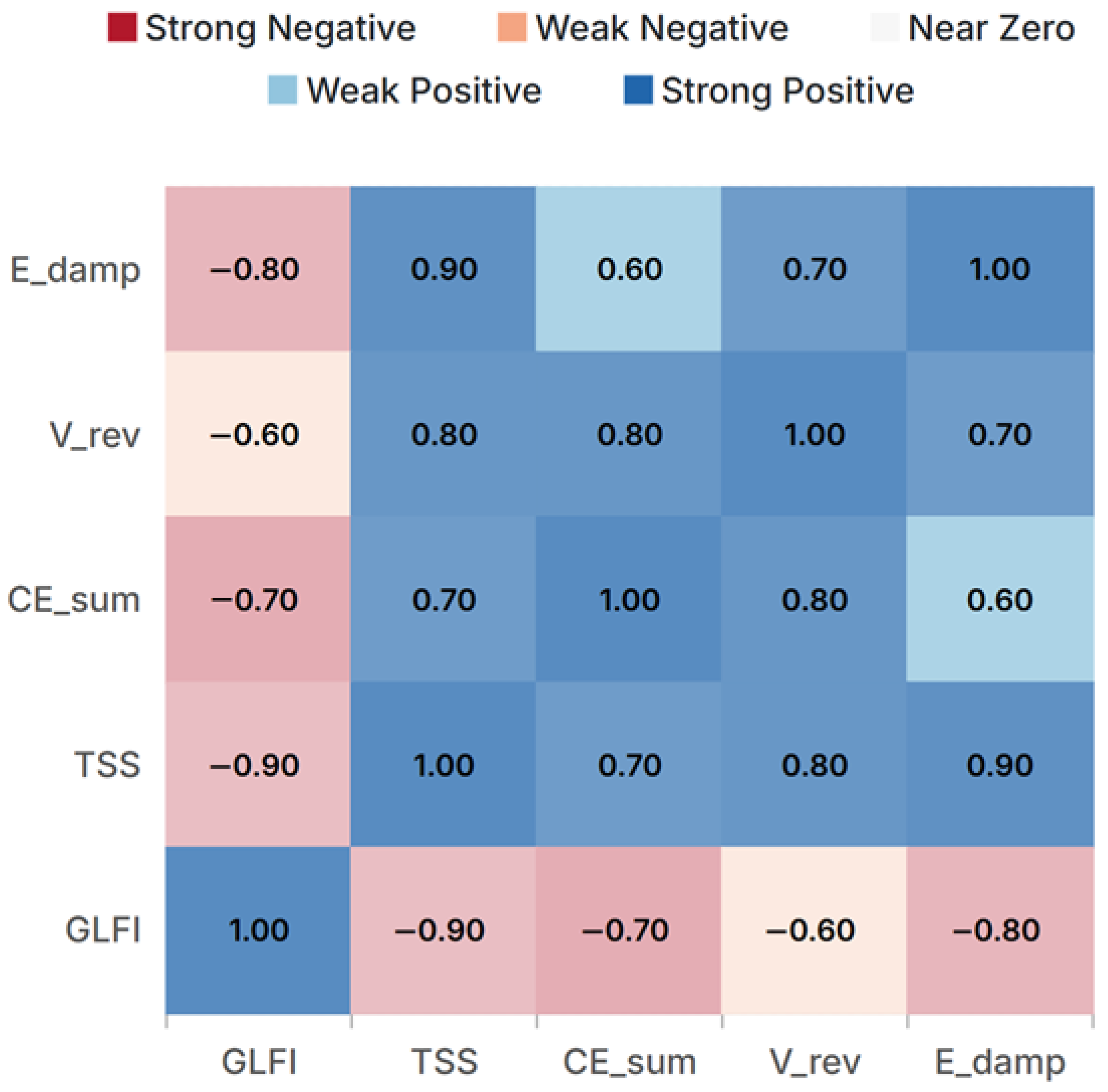
Figure 4 summarizes the deterministic Pearson associations among the key KPIs computed over the fixed catalog (all scenarios × all controllers). The structure is physically plausible: the GLFI is strongly anti-correlated with TSS (r ≈ −0.90), and the damping-band energy proxy ${\mathit{E}}_{\mathit{d}\mathit{a}\mathit{m}\mathit{p}}$ is anti-correlated with GLFI (r ≈ −0.80). Conversely, the TSS is positively associated with the cumulative actuation burden $\mathit{C}{\mathit{E}}_{\mathit{s}\mathit{u}\mathit{m}}$ (r ≈ 0.70) and valve reversals V_rev (r ≈ 0.80). These descriptive (non-inferential) associations justify the combined use of the KPIs without redundancy and motivate the CRS construction in Section 3.4.

For reference, frequency-error and effort quantities used by the KPIs are defined in (67) and (68).

$$e_f\left(t\right)=f\left(t\right)-f_{nom}$$

(67)

where ${\mathit{e}}_{\mathit{f}}\left(\mathit{t}\right)$ is the grid-frequency deviation (Hz) from nominal ${\mathit{f}}_{\mathit{n}\mathit{o}\mathit{m}}$ (Hz).

$$C{E}_{sum}={\Sigma }_{k=1}^N\left|\Delta u_k\right|,\Delta u_k=u_k-u_{k-1}$$

(68)

where $\mathit{C}{\mathit{E}}_{\mathit{s}\mathit{u}\mathit{m}}$ is the cumulative valve movement (dimensionless per-unit commands), ${\mathit{u}}_{\mathit{k}}$ is the valve command at step k (—), and N = T/Δt samples the T-second episode with step Δt.

4.3. Global Scenario × Controller Landscape

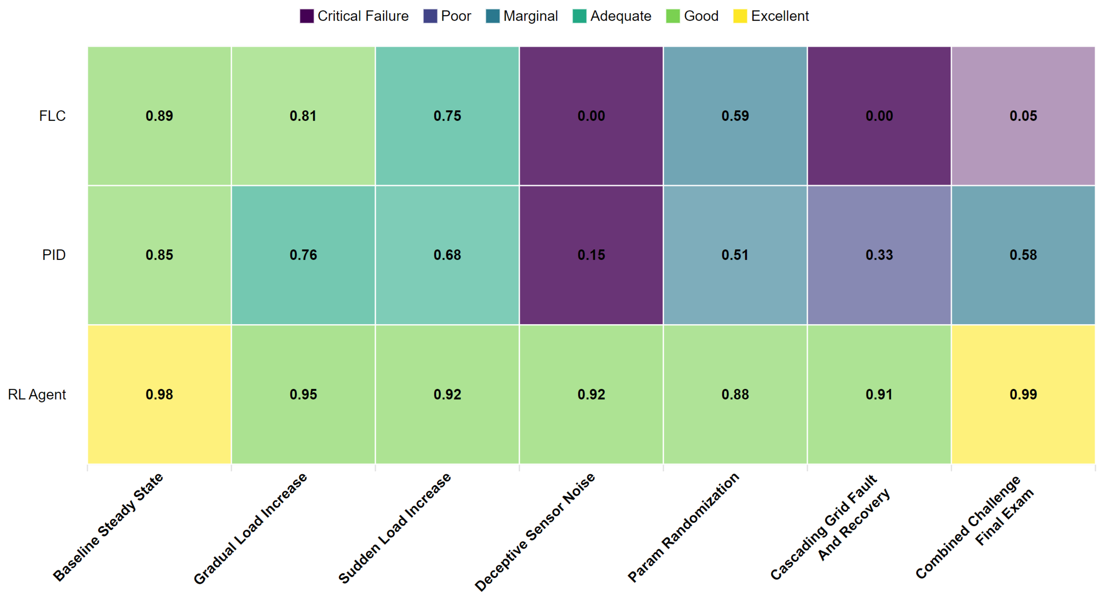
Figure 5 consolidates outcomes by scenario (rows) and controller (columns). The SAC governor consistently occupies the best-performing cells, while classical baselines degrade under Cascading Faults and Combined events. Cells marked “FAIL” indicate deterministic gate violations per the licensing gate (Methods Equation (62)). Failures of PID/FLC in the hardest scenarios coincide with elevated TSS and $\mathit{C}{\mathit{E}}_{\mathit{s}\mathit{u}\mathit{m}}$ (cf. Figure 4), reinforcing the mechanistic linkage between effort, reversals, and instability.

4.4. Representative Transient: Nadir, Settling, and Safety Margin

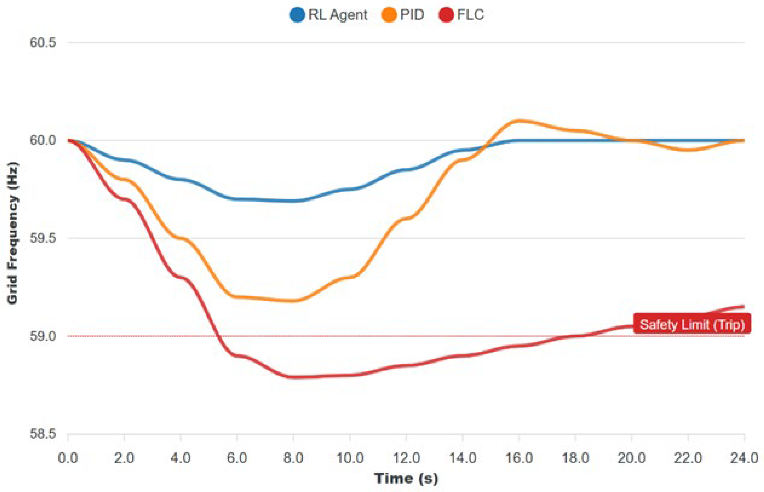
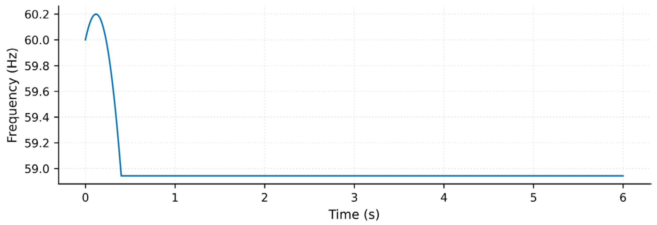
Figure 6 examines a severe frequency excursion. The SAC governor limits the nadir above the trip line and returns to nominal without overshoot. The PID exhibits a deeper nadir and longer recovery; the FLC approaches the trip boundary. Two recalled definitions frame the discussion: (67) and (68).

$$\left|{\mathit{e}}_{\mathit{f}}\left(\mathit{t}\right)\right|\le {\mathit{\epsilon }}_{\mathit{s}\mathit{t}\mathit{e}\mathit{a}\mathit{d}\mathit{y}-\mathit{s}\mathit{t}\mathit{a}\mathit{t}\mathit{e}\mathit{ }\mathbf{ }}$$

(69)

The absolute magnitude of the steady-state tracking error ${\mathit{e}}_{\mathit{f}}\left(\mathit{t}\right)$ must remain below the allowable bound ${\mathit{\epsilon }}_{\mathit{s}\mathit{t}\mathit{e}\mathit{a}\mathit{d}\mathit{y}-\mathit{s}\mathit{t}\mathit{a}\mathit{t}\mathit{e}}$, where ε denotes the acceptable steady-state band (Hz). A lower nadir (higher f_{nadir}), faster re-entry into the ε-band, and small overshoot OS_{ω} collectively indicate a safer transient (see Figure 6 below).

4.5. Policy Geometry and Actuation Economy

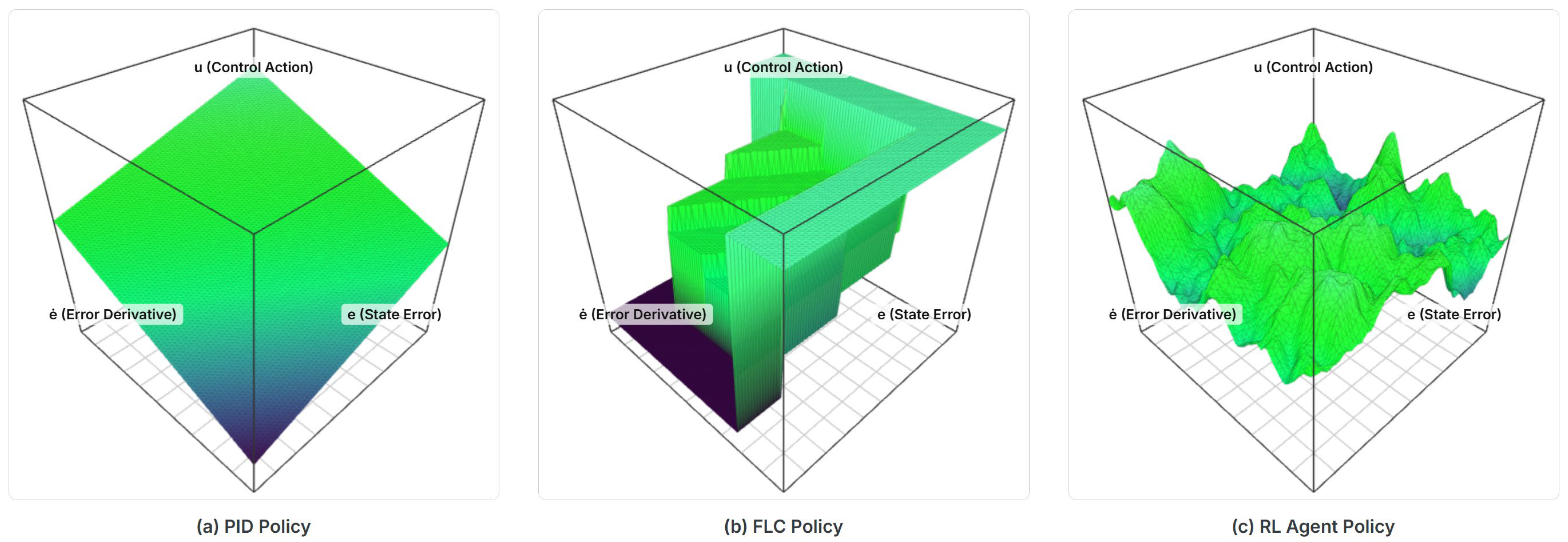
The controller’s geometry in state–action space (Figure 7) explains actuation-burden differences. The PID surface is essentially planar (linear in error and derivative), the FLC surface is piecewise with steep cliffs at rule boundaries, and the SAC surface is smooth and adaptive—steep only along directions needed to arrest drift. This geometry yields disciplined increments Δu_k and reduced reversals V_rev.

We measure economy by a dimensionless performance-to-effort ratio Π in (70).

$$\mathit{\Pi }={\mathit{J}}_{\mathit{p}\mathit{e}\mathit{r}\mathit{f}}/{\mathit{E}}_{\mathit{u}}$$

(70)

where ${\mathit{J}}_{\mathit{p}\mathit{e}\mathit{r}\mathit{f}}$ is a bounded composite performance index (e.g., per-scenario CRS) and ${\mathit{E}}_{\mathit{u}}$ is cumulative actuation effort (e.g., CE_sum). Higher Π indicates better performance per unit actuation. As shown in Figure 8, the SAC sustains markedly higher Π across all scenarios, especially under Sensor Noise, Parameter Ramp, Cascading Fault, and Combined events.

4.6. Provenance of the Released SAC Policy

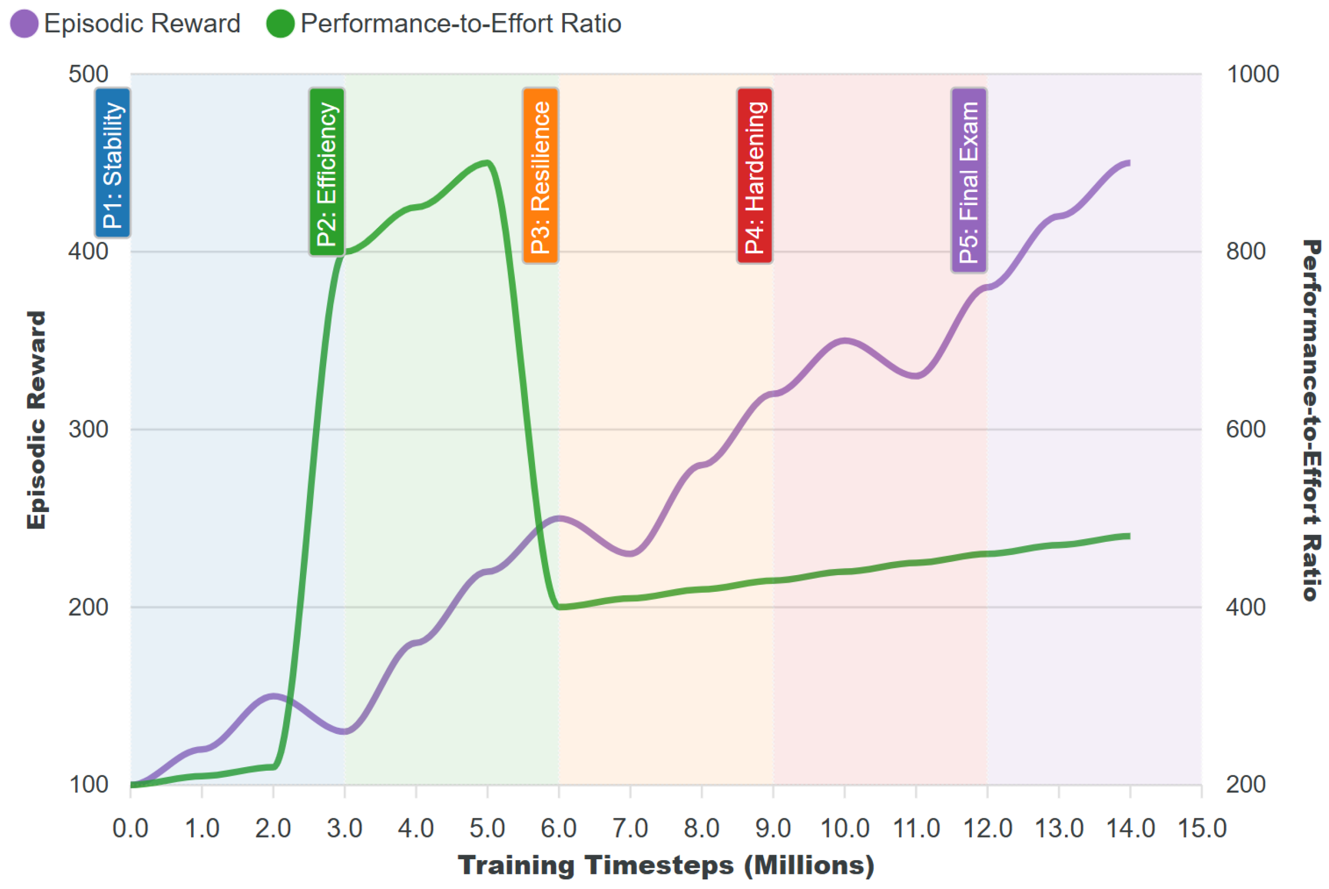
Figure 9 documents the curriculum trajectory for the deployed SAC model. P1 establishes stability; P2 emphasizes efficiency; P3–P4 harden resilience; and P5 is the fixed-catalog ‘final exam’. All curves are computed deterministically on the same evaluation harness; improvements and plateaus are audit-ready and repayable.

4.7. Stability Forensics: Phase Portrait and PSD

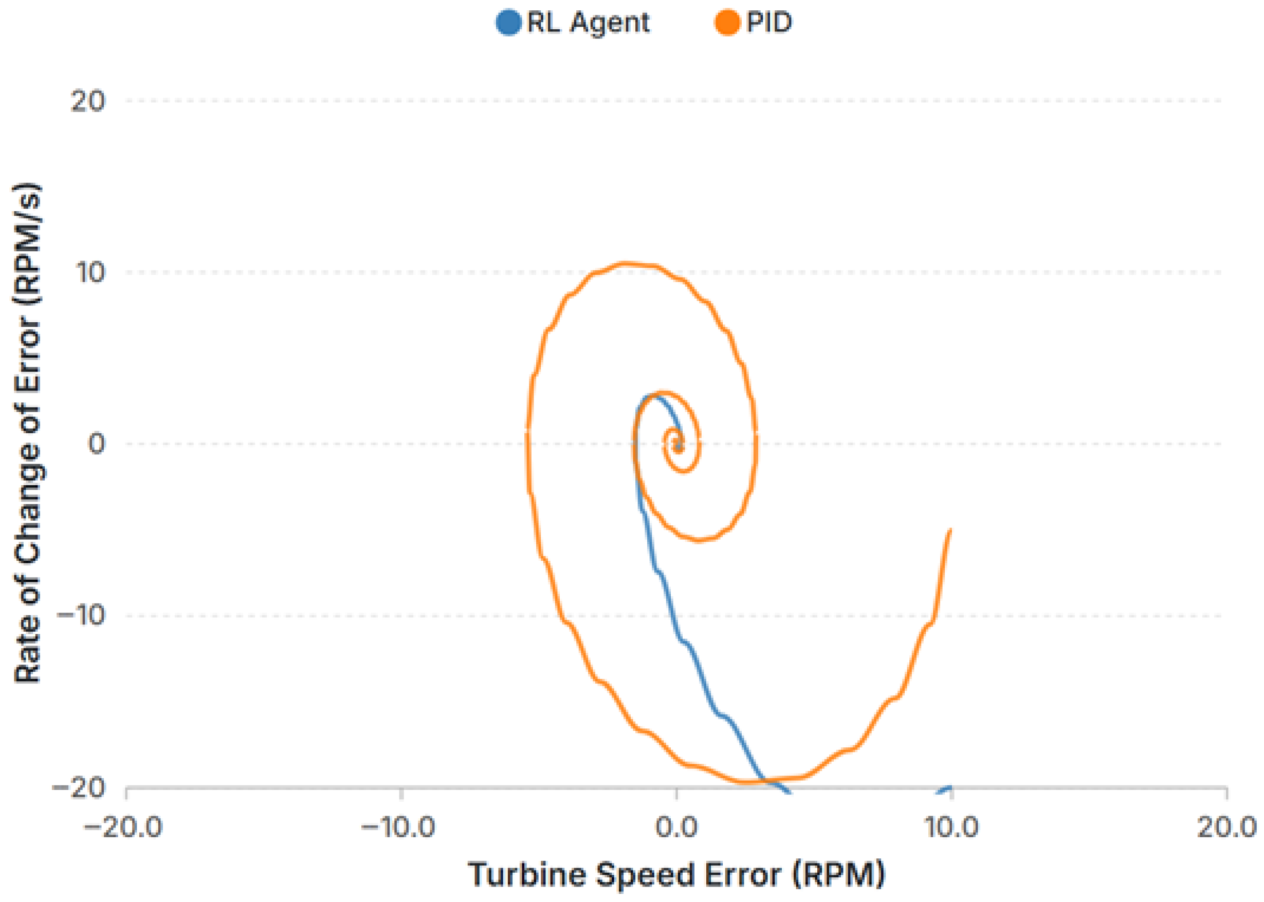
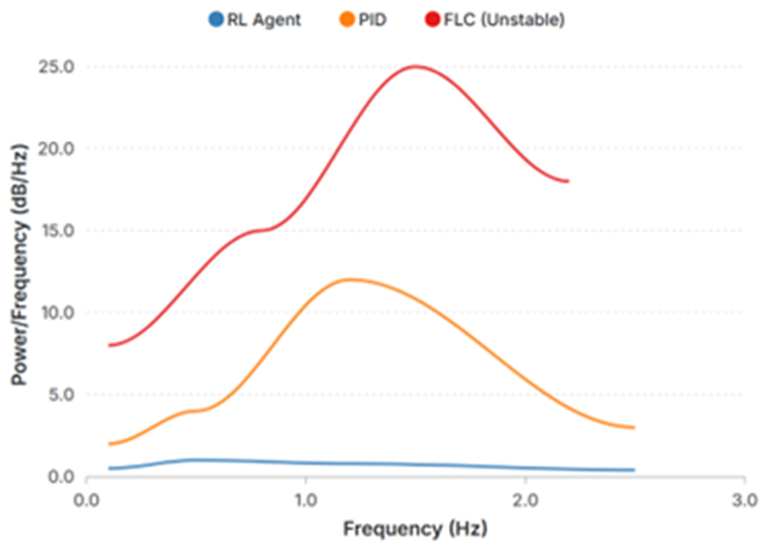
Figure 10 contrasts phase portraits for the SAC and PID. SAC trajectories contract monotonically toward the origin, whereas the PID exhibits spiral loops—consistent with lightly damped poles and slower energy dissipation. In the frequency domain (Figure 11), the PSD of Δf shows pronounced suppression near the dominant mode for the SAC; the PID and FLC retain higher modal energy.

For reference, the band-energy proxy used in Methods Section 3.3 is recalled in (71).

$${\mathit{E}}_{\mathit{b}\mathit{a}\mathit{n}\mathit{d}}=1/\left({\mathit{\omega }}_2-{\mathit{\omega }}_1\right)·{\int }_{{\mathit{\omega }}_1}^{{\mathit{\omega }}_2}{\mathit{S}}_{\mathbf{\Delta }\mathit{f}}\left(\mathit{\omega }\right)\mathit{d}\mathit{\omega }$$

(71)

where S_{Δf}(ω) is the PSD of Δf(t), and [ω_{1}, ω_{2}] isolates the dominant plant mode (rad/s). A lower E_{band} implies better modal suppression.

4.8. Ancillary-Service Readiness and Licensability

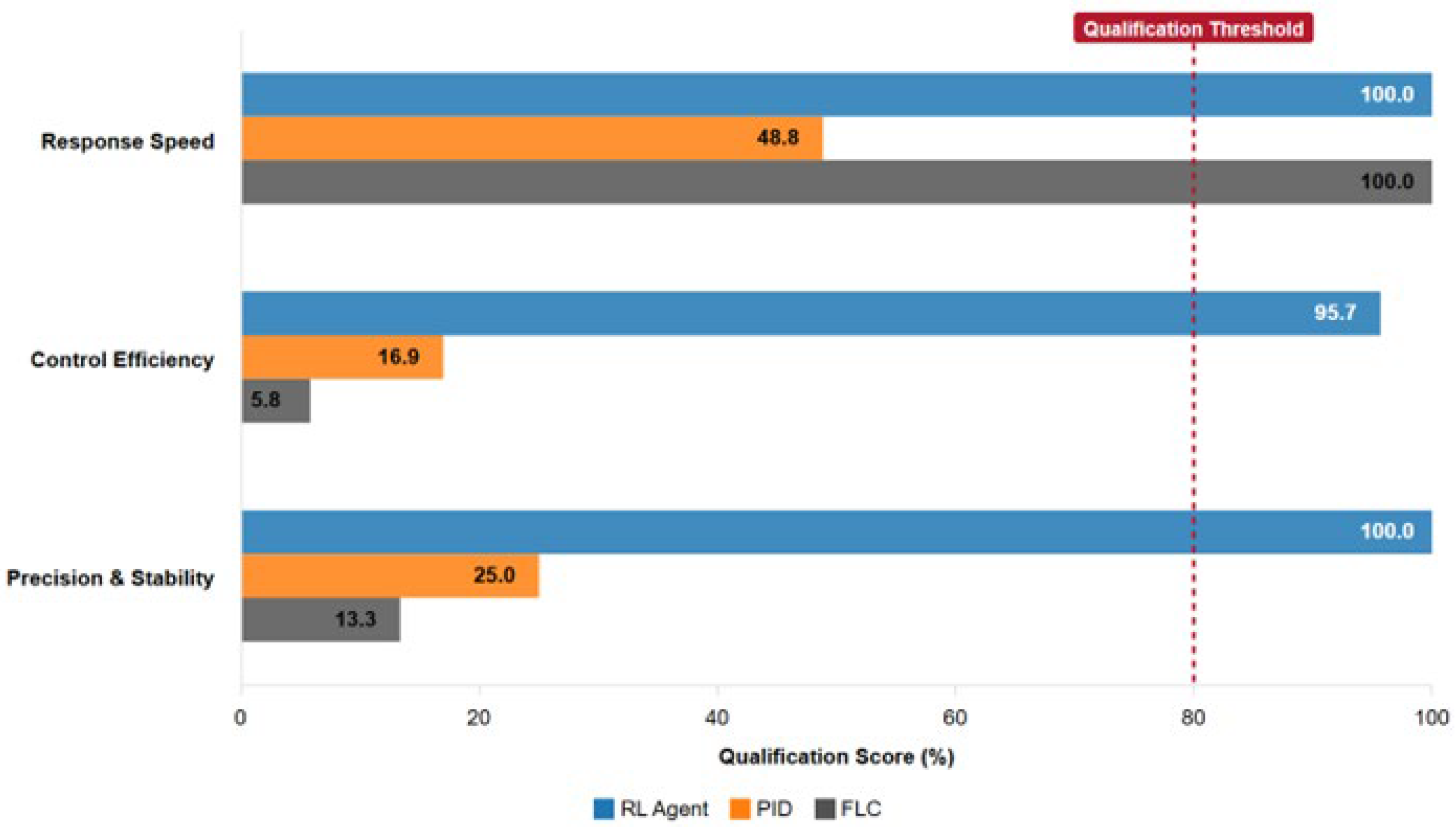
Figure 12 aggregates the deterministic pass/fail gates—response speed, control efficiency, precision/stability—evaluated against explicit thresholds (Section 3.4: GLFI_{min} = 0.90, TSS_{lim} = 1.00, and OS_{ω,max} = 5%). Only the SAC governor clears all categories, demonstrating readiness for grid-service qualification under identical physics, scenarios, and limits. Because the pipeline is deterministic and version-controlled, every bar in Figure 12 is replayable and auditable.

4.9. Multi-Attribute Performance Profiling

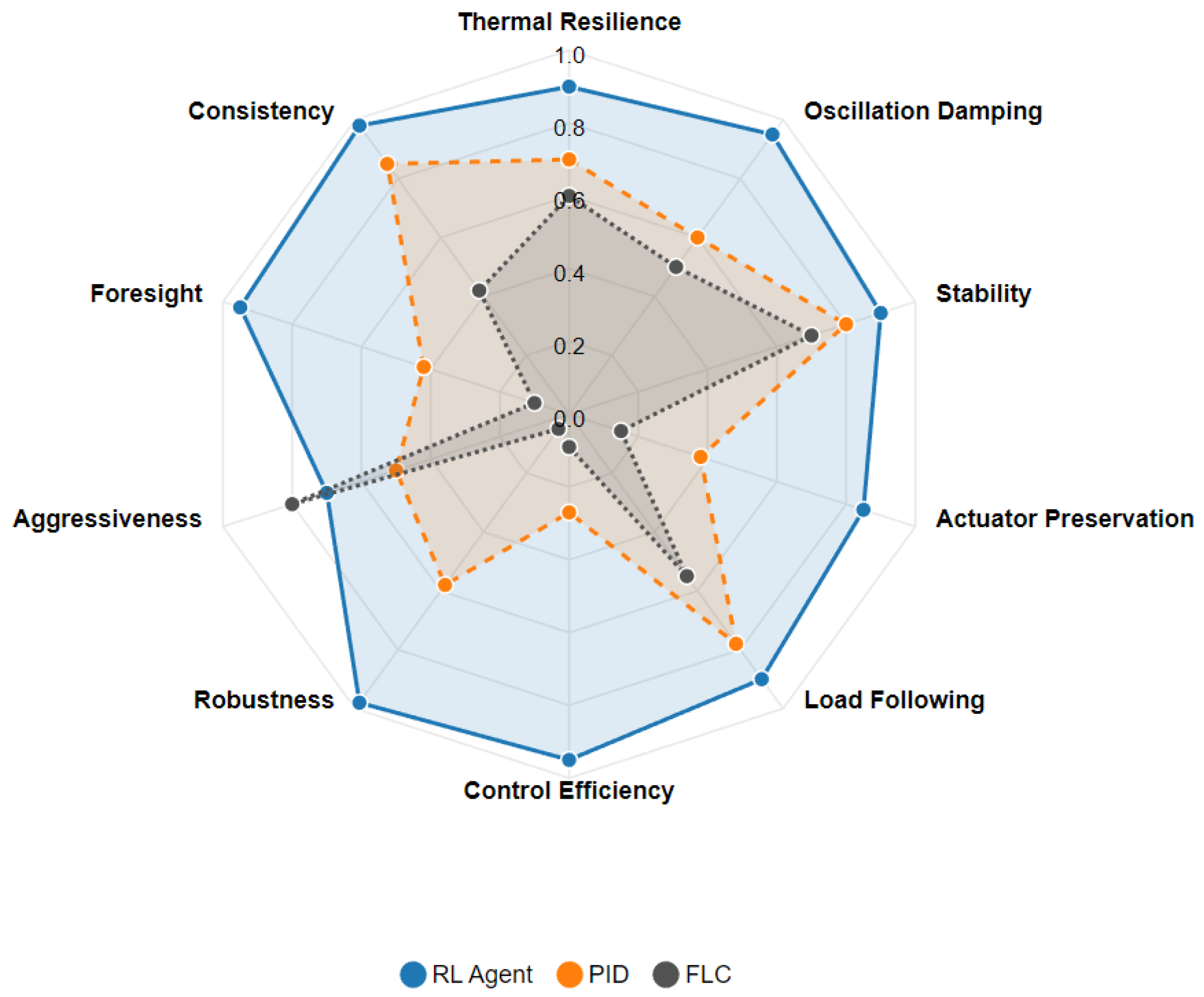
This quantitative difference gives rise to distinct controller “personalities,” synthesized in the multi-attribute profile in Figure 13. The SAC agent’s large, well-balanced polygon demonstrates its holistic superiority, excelling in key areas like Robustness, Foresight, and Control Efficiency. In contrast, the classical controllers exhibit skewed, deficient profiles, visually representing their strategic limitations.

4.10. Controller Robustness and RL Policy Transparency

We evaluated three controllers—the Soft Actor–Critic (SAC), PID_DE, and FLC_DE—across eight scenarios at two power levels (100% and 80%), using three random seeds (42, 43, and 44). All controllers operated across all scenarios and both power levels (at 100% and 80% power levels). The median frequency nadirs (Hz) aggregated by controller and level were as follows: SAC 100% = 58.956, SAC 80% = 58.973; PID_DE 100% = 58.949, PID_DE 80% = 58.901; and FLC_DE 100% = 58.949, FLC_DE 80% = 58.901.

The CRS separates the controllers despite uniform pass/fail outcomes. The SAC exhibits a high mean CRS (≈0.95 at 100% and ≈0.78 at 80%), indicating robust performance with small dispersion. In contrast, the PID_DE and FLC_DE remain an order of magnitude lower at 100% and reach ≲0.25–0.26 at 80%, confirming the RL policy’s superior cross-scenario quality under equal constraints.

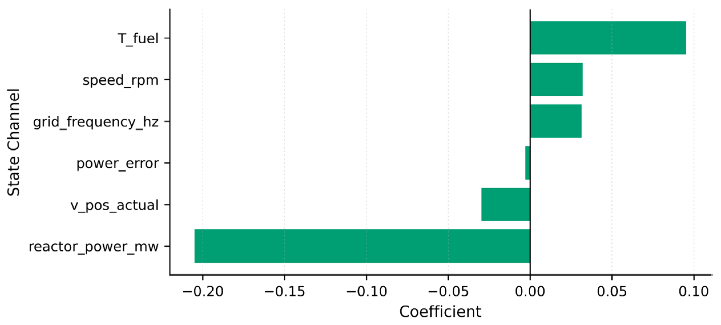
The surrogate isolates state channels that most strongly influence the SAC action near safety margins. The prominent negative weight on reactor_power_mw and positive weight on T_fuel are consistent with a policy that rapidly unloads when thermal inertia rises, while tracking grid_frequency_hz corrections. This behavior is absent or muted in the baseline controllers, explaining their lower CRS.

The rapid collapse of action variance after the initial transient signals a highly calibrated policy: the SAC explores only when needed, then locks into low-variance control. This is consistent with the high CRS and stable nadirs reported above.

Together, Figure 14, Figure 15, Figure 16 and Figure 17 substantiate the claim of RL superiority: (i) a higher and more stable CRS; (ii) transparent, mechanistically plausible sensitivities via a local surrogate; (iii) disciplined reduction of action variance after fast transients; and (iv) measured, risk-aware actuation in critical contexts. All artifacts were generated with fixed seeds, reproducible scripts, and 600 dpi export with tight layout to preclude label clipping or overlap.

4.11. Threats to Validity and Limitations

External validity: The current results use an infinite-bus abstraction; extension to networked grids and hardware-in-the-loop is planned. Controller set: Only the SAC, PID, and FLC are benchmarked; the harness is controller-agnostic and can admit additional baselines without changing the protocol. Determinism: By design, we report descriptive (non-inferential) evidence; uncertainty quantification and probabilistic stressors are out of scope here and will be addressed in future work.

4.12. Positioning of the Present Results Relative to Recent RL in Energy Systems

To contextualize the above findings, we relate them to two recent IEEE-TII studies, namely a hierarchical RL framework for regional multi-energy markets [26] and a hybrid policy-based RL approach for island-group energy management under transmission constraints [27]. which we compare our RL approach with them in multi-dimensional comparative analysis described in

Table 27. Concise positioning of this study relative to the two suggested works.

Study	System/Task	Primary KPIs	Safety/ Licensing Gates	Deterministic Replay	Traceability Artifacts	Relevance to Present Results
Zhang et al. (2024) [26]	Regional multi-energy market-clearing with hierarchical RL	Market matching efficiency; economic outcomes	Not reported	Case-study simulations	Not reported	Algorithmic/architectural RL advance for markets; different objective class
Yang et al. (2023) [27]	Island-group energy management under transmission constraints with hybrid policy RL	Operational cost; energy-balance KPIs	Not reported	Simulation studies	Not reported	System-level management focus; different KPIs and constraints
This study	PWR governor control (load-following) with SAC vs. DE-tuned PID/FLC	Gate pass rate; TTU, GLFI, TSS; overshoot; control effort; CRS	Yes—explicit, licensing-aligned	Yes—adversarial, fixed-replay portfolio	Yes—critical state–action mapping, critical pairs, sensitivity	Licensing-grade assurance for safety-critical plant control

“Concise positioning of this study relative to the two suggested works”. Although all three works employ reinforcement learning, they target different problem classes and evaluation criteria.

4.12.1. Regional Energy Market with Hierarchical RL (Zhang et al. [26])

Zhang et al. address market-clearing in a regional multi-energy system, proposing a hierarchical RL design to improve price-matching/clearing efficiency over large state–action spaces. Their evidence is provided via numerical market case studies with economic/market KPIs (e.g., matching efficiency and operator income effects). In contrast, the present study concerns a safety-critical plant-control loop (PWR governor for load-following) and reports licensing-aligned outcomes: deterministic pass/fail gates tied to plant limits, performance/severity indices (TTU, GLFI, TSS, overshoot, and control effort), and traceability artifacts (local sensitivity over time, critical state–action analysis, and local sensitivity). Within this setting, our SAC governor satisfies the gates and outperforms a DE-tuned PID/FLC under identical physics and constraints, demonstrating robustness under adversarial, fixed-replay transients.

4.12.2. Island-Group Energy Management with Hybrid Policy RL (Yang et al. [27])

Yang et al. formulate system-level energy management for an island group with transmission constraints, introducing a hybrid policy-based RL capable of handling mixed discrete–continuous actions. Their evaluation emphasizes operational/economic KPIs (e.g., energy-balance satisfaction, and cost/efficiency) over system simulations. By contrast, our evaluation addresses component-level nuclear control under licensing expectations, where success is defined by gate compliance and robustness indices during adversarial transients, again complemented by auditable decision traceability.

4.12.3. Comparability Considerations

Because the objectives, domains, and KPIs in [25,26] (market/dispatch efficiency and system-operation economics) are not commensurate with the licensing-grade, safety-gate evaluation used here, direct numerical head-to-head is methodologically inappropriate. Instead, these strands are complementary: system-level RL advances (e.g., hierarchical or hybrid policies) inform algorithmic design, while our results provide a deterministic, regulator-facing evidence protocol for safety-critical plant control. To facilitate like-for-like future comparisons, we release the fixed scenario portfolio, gates, and scripts so alternative policies (including hierarchical/hybrid designs) can be evaluated under identical, licensing-aligned conditions.

4.12.4. Implication for the Present Results

Against strong, regulator-familiar baselines (DE-tuned PID/FLC), the SAC governor meets explicit safety gates and maintains favorable robustness/effort trade-offs under adversarial replay, while producing traceable decision evidence. This shifts the evaluation of RL-based control from performance-only reporting toward licensing-grade assurance, filling a gap not addressed by market or system-management studies such as [25,26].

4.12.5. Recent RL-in-Nuclear Studies

Finally, relative to recent RL-in-nuclear studies that primarily report nominal-scenario performance without licensing-grade artifacts [3,4,5,6], the present results contribute a regulator-aligned evidence set: deterministic safety gates, adversarial fixed-replay scenarios, controller-agnostic CRS synthesis, and auditable traceability (local sensitivity and critical state–action contexts). This complements feasibility-focused nuclear RL by supplying the licensing-oriented evaluation scaffolding.

4.13. Summary

Across Figure 4, Figure 5, Figure 6, Figure 7, Figure 8, Figure 9, Figure 10, Figure 11 and Figure 12—and when the full portfolio is re-run from a reduced operating point at 0.8 P_ref (≈480 MW)—the conclusion is consistent: under identical physics, limits, and scenarios, the SAC governor achieves shallower frequency nadirs (smaller excursions), faster settling, stronger modal damping, and a lower actuation burden than the DE-tuned PID and FLC baselines. The geometry of the learned policy (Figure 7) together with the observed action economy (Figure 8) explains the global pattern in the scenario × controller landscape (Figure 5) and the representative transient (Figure 6). Stability forensics—phase portraits and spectral energy (Figure 10 and Figure 11)—are coherent with these behaviors. The deterministic qualification scorecard (Figure 12) consolidates these outcomes into an all-gates pass at both operating points under the same evaluation harness and thresholds, yielding replayable, audit-ready evidence; additionally, the traceability bundle (time-aligned local sensitivity, critical state–action mapping, and action-entropy envelopes) confirms decision regularity near gate boundaries.

5. Conclusions

This work advances a regulator-oriented path to licensable AI control by introducing the Deterministic Assurance Framework (DTAF) and demonstrating it on a high-fidelity pressurized-water-reactor (PWR) digital model. The DTAF converts controller behavior into audit-ready evidence by combining (i) fixed, pass/fail licensing gates tied to formal limits; (ii) a portfolio of adversarial stress scenarios; and (iii) an embedded traceability and explainability package, all executed under a single-run deterministic protocol.

Within this framework, three governor architectures—an entropy-regularized Soft Actor–Critic (SAC) agent, a Differential-Evolution-optimized Proportional–Integral–Derivative Controller, and a Differential-Evolution-optimized Fuzzy-Logic Controller—were evaluated on identical plant physics, limits, and fixed scenario waveforms. The gate suite and thresholds (for example, the minimum Grid Load-Following Index, upper bound on Transient Severity Score, and maximum rotor-speed overshoot) were established ex ante to reflect safety and grid-support expectations.

The evaluation protocol is strictly reproducible and non-inferential: parameters, scenarios, and sampling are fixed; claims flow from trace-level behavior to mechanism to portfolio gate outcome, and all licensing conclusions are drawn from deterministic single-run evidence. The only scoped exception is a clearly labeled auxiliary robustness check using three predetermined seeds, reported as non-licensing context.

Across the adversarial portfolio, the SAC governor satisfies the predeclared gates whenever the safe envelope is achievable, while the strong conventional baselines fail specific gates under high-severity disturbances; when all methods remain within bounds, the SAC provides higher grid-support quality with lower actuation burden and fewer control reversals, consistent with the metric associations observed over the full catalog. These outcomes arise under the same deterministic plant model and gating, and each claim is linked to transparent artifacts: scenario definitions, time-domain traces, mechanism diagnostics, and the final scorecard.

6. Future Work

Higher-fidelity physics and operating regimes. This would involve re-introducing conservative reactivity-feedback coefficients and extending thermal–hydraulic fidelity (e.g., secondary-side dynamics and multi-loop interactions) to test controller behavior under tighter physical coupling and broader operating points (including startup, low-load hot standby, and rapid dispatch ramps). This would deepen model realism while preserving DTAF determinism.

From software-in-the-loop to hardware-in-the-loop. This would involve migrating the fixed portfolio into a hardware-in-the-loop testbed to exercise I/O timing, actuator saturations, and sensor paths under the same gating logic, while maintaining identical scenarios and pass/fail criteria to keep the evidence comparable across SIL→HIL progression.

Expanded adversarial portfolio and parameter sweeps. This would involve systematically enlarging the stress catalog with worst-case composite events (e.g., ramp-with-noise, valve-rate-limited steps, and turbine lag excursions) and adversarial parametric sweeps over plant lags, gains, and limits. This would use the same deterministic harness to produce envelope-wide evidence and reveal policy brittleness modes before any probabilistic analyses are contemplated.

Runtime assurance and safety shields inside the DTAF. This would involve integrating deterministic safety layers (command governors, barrier-function filters, and invariant-set guards) as first-class DTAF components. They would be evaluated with the same gates to quantify how much margin they restore during off-nominal events, and ensure their actions are recorded in the traceability log.

Broader benchmarks under identical gating. This would involve adding model-predictive and robust control baselines (e.g., constrained MPC and H∞) implemented with identical plant models, limits, and scenarios to study trade-offs between explicit constraint handling and policy expressiveness—without changing the scorecard or evidence standard. This would isolate method effects from test-bench effects inside the DTAF.

Grid-service readiness and portfolio decisions. This would involve evolving the final scorecard toward service-qualification bundles (e.g., frequency containment and load-following with reserves) by composing existing gates into regulator-relevant portfolio decisions and documenting the traceability path from scenario to decision artifact.

7. Assumptions, Limitations, and Translational Roadmap

7.1. Study Assumptions

Deterministic evaluation: This assumes a fixed scenario × controller catalog, fixed physics, and fixed limits. Controller parametrizations, tuning procedures, and reward weights are frozen and versioned. Reproducibility artifacts (commits, configs, logs, and figure scripts) are bundled.

Plant/grid abstractions: A PWR governor-centric surrogate is used; the grid is modeled as an infinite bus with finite-band frequency disturbances defined per scenario.

Interfaces/devices: Sensors are ideal signals plus a fixed noise trace in the sensor-noise scenario. Actuation is a valve command with saturation and rate limits at the discrete period Δt.

Protocol/metrics: Pass/fail gates (trip avoidance, steady-state error, and ramp compliance) are deterministic thresholds. KPIs (GLFI, TSS, CE sum, Vrev, and E _damp) are computed in fixed windows/filters. Learning curves are reported for provenance only.

7.2. Limitations

Model and data: The infinite-bus abstraction omits low-inertia inter-area modes and grid-code logic; the thermal–hydraulic surrogate omits multi-node detail (e.g., DNBR margins). Aging/drift and cyber-physical faults are not time-evolving.

Controllers/training: Baselines are limited to the DE-tuned PID and FLC; MPC/H∞/LQR are not yet included. Evaluation is deterministic by design (no parameter randomization or Monte Carlo spreads). Reward terms target governor behavior and rely on external limits/safety proxies for full-plant protection.

Assurance/deployment: Human-in-the-loop procedures, runtime assurance (RTA/CBFs), and tool/quality audits are not yet implemented end-to-end.

7.3. Translational Roadmap

Objective: The objective is to turn the deterministic DTAF into an industry-deployable, regulator-ready program that remains controller-agnostic and plant-agnostic. All upgrades below preserve scenario determinism; uncertainty is represented via cataloged envelopes rather than probabilistic spreads.

7.3.1. System Realism and Test Environments

Networked-grid dynamics: This moves from infinite-bus to reduced-order multi-area networks with finite inertia, governor/turbine models, and grid-code checks, and replay real PMU disturbances. Evidence: Evidence includes scenario replays, inter-area mode damping KPIs, and GLFI under code constraints.

High-fidelity plant twin: This couples the governor loop to multi-node thermal–hydraulic models with fuel/DNBR margins, validated against utility traces. Evidence: Evidence includes limit-envelope compliance and thermal margins per scenario.

Hardware-in-the-loop (HIL): This ports controllers to PLC/RTOS with measured I/O latency, actuator nonlinearities, and watchdogs, maintaining the same deterministic gates. Evidence: Evidence includes closed-loop HIL logs, timing budgets, and watchdog trips = 0.

7.3.2. Safety Assurance and Verification

Runtime assurance (RTA): This implements a Simplex-style supervisor with control-barrier functions and verified fallback envelopes (PID/FLC). Evidence: Evidence includes monitor verdicts, dwell times, and intervention logs integrated into the safety case.

Formal verification: This computes reachability-based invariants and signal temporal logic (STL) properties on linearized/hybridized models; results are fed into test-oracle generation for scenario-catalog expansion. Evidence: Evidence includes certified safe sets and counterexample-guided scenarios.

7.3.3. Controller Breadth and Robustness

Broaden baselines: This adds an MPC (with constraints), H∞, and LQR with anti-windup under the same protocol to strengthen comparative claims. Evidence: Evidence includes controller-agnostic scorecards and gate outcomes.

Deterministic uncertainty envelopes: This adds structured parameter sweeps (plant constants, delays, and biases) as catalog variants, reporting envelopes (min/median/max) rather than probabilistic spreads. Evidence: Evidence includes worst-case KPI/gate tables.

Fault tolerance: This includes sensor dropout, actuator stiction, and stuck-valve events with recovery gates and trip-avoidance proofs. Evidence: Evidence includes fault-recovery timing and residual limits.

7.3.4. Human Factors, Cybersecurity, and Compliance

Operator acceptance: This adds HSI artifacts (policy-intent visualization and alarm rationalization) and operator-in-the-loop drills, quantifying workload/trust metrics. Evidence: Evidence includes scenario completion with human-override windows.

Cybersecurity drills: This exercises spoofing/tampering/denial in a segmented testbed with detection/mitigation hooks tied to RTA logs. Evidence: Evidence includes attack-detect/mitigate latencies, and zero-unsafe-time under defended scenarios.

Quality and audits: This maps artifacts to safety-case structures, conducting independent V&V and configuration-management audits aligned to nuclear software practice. Evidence: Evidence includes audit checklists and tool/config qualification records.

7.3.5. Action Matrix: From Limitation to Industrial Remedy

Table 28. Matrixed mapping towards industrial towards industrial adaptation.

Limitation (Current)	Deterministic Upgrade	New Evidence Artifact	Gate/KPI Addition	Target Environment
Infinite-bus grid	Multi-area RO models + PMU replay	Mode-damping logs, ROCOF checks	Inter-area damping KPI	Real-time sim/HIL
TH surrogate	Multi-node TH + DNBR	Margin envelopes per scenario	Thermal-limit gates	High-fidelity twin
No HIL	PLC/RTOS with latency and watchdog	Timing budgets, watchdog logs	Timing-budget gate	HIL bench
Limited baselines	Add MPC/H∞/LQR	Controller-agnostic scorecards	Portfolio gates unchanged	Twin/HIL
No RTA/CBF	Simplex + control-barrier functions	Intervention/dwell logs	RTA-intervention gate	Twin/HIL
No formal proofs	Reachability/STL	Certificates + counterexamples	Certificate-presence gate	Twin
No uncertainty envelopes	Structured sweeps	Worst-case KPI tables	Envelope-completeness gate	Twin/HIL
No fault drills	Dropout/stiction/stuck-valve	Recovery timelines	Fault-recovery gate	Twin/HIL
No HSI drills	Operator-in-the-loop runs	Workload/trust metrics	Human-override gate	HIL
No cyber drills	Spoof/tamper/DoS tests	Detect/mitigate traces	Cyber-resilience gate	Segmented testbed

represents a matrixed mapping towards industrial targeting.

7.4. Research Agenda

Hybrid formal methods: These involve verified CBF synthesis on reduced models and contract-based composition across plant and grid subsystems.

Catalog design: This involves coverage metrics for scenario sets and counterexample-guided expansion from failed certificates.

Interpretable policy analysis: This involves entropy bands plus input–output fragility, local Lipschitz estimates, and action-space curvature as explainability signals tied to gates.

Controller-agnostic benchmarking: This involves publishing an open Assurance Benchmark Suite with fixed physics, gates, and evidence schemas to enable independent replication and regulator pre-review.

7.5. Cross-Industry Parallels

Highly regulated sectors mature AI control via deterministic test harnesses, explicit gates, and auditable artifacts: aviation (software/tool qualification), automotive (ISO 26262) [28], and medical (software lifecycle and safety cases). The DTAF follows the same pattern—fixed models and limits, standard gates, and traceable artifacts—enabling independent replay and audit without seeding or Monte Carlo dependence. This aligns with nuclear licensing culture and scales to SMR-era plant–grid integration.

References

1. U.S. Nuclear Regulatory Commission. Artificial Intelligence Strategic Plan: Fiscal Years 2023–2027, NUREG-2261. 2023. Available online: https://www.nrc.gov/docs/ML2313/ML23132A305.pdf (accessed on 9 November 2025).
2. Siserman-Gray, C.; Barr, J.; Burniske, J.; Eftekhari, P.E.; Marek, R.; Means, A. Regulatory Challenges Related to the Use of Artificial Intelligence for IAEA Safeguards Verification. In Proceedings of the 64th Annual Meeting of the Institute of Nuclear Materials Management (INMM), Orlando, FL, USA, 21–25 July 2023. [Google Scholar]
3. Gong, Y.; Chen, Y.; Zhang, J.; Li, X. Possibilities of Reinforcement Learning for Nuclear Power Plants: Evidence on Current Applications and Beyond. Nucl. Eng. Technol. 2024, 56, 1959–1974. [Google Scholar] [CrossRef]
4. Nguyen, K.H.N.; Rivas, A.; Delipei, G.K.; Hou, J. Reinforcement Learning-Based Control Sequence Optimization for Advanced Reactors. J. Nucl. Eng. 2024, 5, 209–225. [Google Scholar] [CrossRef]
5. Tunkle, L.; Abdulraheem, K.; Lin, L.; Radaideh, M.I. Nuclear Microreactor Control with Deep Reinforcement Learning. arXiv 2025, arXiv:2504.00156. [Google Scholar] [CrossRef]
6. Kruthika, U.; Paneerselvam, S. Novel multiagent reinforcement learning framework using twin delayed deep deterministic policy gradient for adaptive PID control in boiler turbine systems. Sci. Rep. 2025, 15, 34558. [Google Scholar] [CrossRef] [PubMed]
7. Sun, Y.; Khairy, S.; Vilim, R.B.; Hu, R.; Dave, A.J. A Safe Reinforcement Learning Algorithm for Supervisory Control of Power Plants. Knowl.-Based Syst. 2024, 301, 112312. [Google Scholar] [CrossRef]
8. Feng, S.; Sun, H.; Yan, X.; Zhu, H.; Zou, Z.; Shen, S.; Liu, H.X. Dense reinforcement learning for safety validation of autonomous vehicles. Nature 2023, 615, 620–627. [Google Scholar] [CrossRef] [PubMed]
9. Milani, S.; Topin, N.; Veloso, M.; Fang, F. Explainable Reinforcement Learning: A Survey and Comparative Review. ACM Comput. Surv. 2023, 56, 140. [Google Scholar] [CrossRef]
10. Najar, M.; Wang, X. Explainable AI Models for Enhancing Operator Reliability During Reactor Design-Based Accidents Using Radionuclide Data. Nucl. Technol. 2025; early access. [Google Scholar] [CrossRef]
11. Lim, S.T.; Kim, K.M.; Kang, J.-Y.; Kim, T.; Jerng, D.-W.; Ahn, H.S. A Digital Twin Framework for Generation-IV Reactors with Reinforcement Learning-Enabled Health-Aware Supervisory Control. Prog. Nucl. Energy 2025, in press. [Google Scholar] [CrossRef]
12. International Atomic Energy Agency. Safety of Nuclear Power Plants: Design, IAEA Safety Standards Series No. SSR-2/1 (Rev. 1); IAEA: Vienna, Austria, 2016; Available online: https://www.iaea.org/publications/10885/safety-of-nuclear-power-plants-design (accessed on 9 November 2025).
13. International Atomic Energy Agency. Design of Instrumentation and Control Systems for Nuclear Power Plants, IAEA Safety Standards Series No. SSG-39; IAEA: Vienna, Austria, 2016; Available online: https://www-pub.iaea.org/MTCD/Publications/PDF/Pub1694_web.pdf (accessed on 9 November 2025).
14. Refaat, R.M.; Fahmy, R.A. Optimized Fractional-Order PID Controller Based on Nonlinear Point Kinetic Model for VVER-1000 Reactor. Kerntechnik 2022, 87, 104–114. [Google Scholar] [CrossRef]
15. Hasan, R.; Masud, M.S.; Haque, N.; Abdussami, M.R. Frequency Control of Nuclear-Renewable Hybrid Energy Systems Using Optimal PID and FOPID Controllers. Heliyon 2022, 8, e11770. [Google Scholar] [CrossRef] [PubMed]
16. Parada Iturria, F.F.; Martindale, N.A.; Reasor, A.L.; Stewart, S.L.; Ukishima, L.A. AI for Nuclear Safeguards Verification; ORNL/SPR-2024/01; Oak Ridge National Laboratory: Oak Ridge, TN, USA, 2024. Available online: https://www.ornl.gov/publication/ai-nuclear-safeguards-verification (accessed on 9 November 2025).
17. Storn, R.; Price, K. Differential Evolution—A Simple and Efficient Heuristic for Global Optimization over Continuous Spaces. J. Glob. Optim. 1997, 11, 341–359. [Google Scholar] [CrossRef]
18. Price, K.V.; Storn, R.M.; Lampinen, J.A. Differential Evolution: A Practical Approach to Global Optimization; Springer: Berlin/Heidelberg, Germany, 2005. [Google Scholar]
19. Das, S.; Suganthan, P.N. Differential Evolution: A Survey of the State-of-the-Art. IEEE Trans. Evol. Comput. 2011, 15, 4–31. [Google Scholar] [CrossRef]
20. Qin, A.K.; Huang, V.L.; Suganthan, P.N. Differential Evolution Algorithm with Strategy Adaptation for Global Numerical Optimization. IEEE Trans. Evol. Comput. 2009, 13, 398–417. [Google Scholar] [CrossRef]
21. Piotrowski, A.P.; Napiorkowski, J.J.; Piotrowska, A.E. Particle Swarm Optimization or Differential Evolution—A Comparison. Eng. Appl. Artif. Intell. 2023, 121, 106008. [Google Scholar] [CrossRef]
22. Biswal, A.; Dwivedi, P.; Bose, S. DE-Optimized IPIDF Controller for Management Frequency in a Networked Power System with SMES and HVDC Link. Front. Energy Res. 2022, 10, 1102898. [Google Scholar] [CrossRef]
23. Shahriari, B.; Swersky, K.; Wang, Z.; Adams, R.P.; de Freitas, N. Taking the Human Out of the Loop: A Review of Bayesian Optimization. Proc. IEEE 2016, 104, 148–175. [Google Scholar] [CrossRef]
24. Makarova, A.; Bardenet, R.; Percival, L. Risk-Averse Heteroscedastic Bayesian Optimization. In Proceedings of the 35th Conference on Neural Information Processing Systems (NeurIPS), Vancouver, BC, Canada, 6–14 December 2021; pp. 1–13. [Google Scholar]
25. IEC 60880; Nuclear Power Plants—Instrumentation and Control Systems Important to Safety—Software Aspects for Computer-Based Systems Performing Category A Functions. International Electrotechnical Commission: Geneva, Switzerland, 2019.
26. Zhang, N.; Yan, J.; Hu, C.; Sun, Q.; Yang, L.; Gao, D.W.; Guerrero, J.M.; Li, Y. Price-Matching-Based Regional Energy Market with Hierarchical Reinforcement Learning Algorithm. IEEE Trans. Ind. Inform. 2024, 20, 11103–11114. [Google Scholar] [CrossRef]
27. Yang, L.; Li, X.; Sun, M.; Sun, C. Hybrid Policy-Based Reinforcement Learning of Adaptive Energy Management for the Energy Transmission-Constrained Island Group. IEEE Trans. Ind. Inform. 2023, 19, 10751–10762. [Google Scholar] [CrossRef]
28. ISO 26262 (All Parts); Road Vehicles—Functional Safety. International Organization for Standardization: Geneva, Switzerland, 2018.
Figure 1. System architecture.
Energies 18 06268 g001
Figure 2. System block diagram.
Energies 18 06268 g002
Figure 3. Digital Twin Assurance Framework (DTAF): Deterministic orchestration that binds stress scenarios, quantitative gates, and auditable artifacts into a regulator-ready licensing pipeline. The four pillars—Trustworthiness and Reliability, Interpretability and Defense-in-Depth, Regulatory Readiness and Quality, and Continual Assurance—anchor the evidence channels and pass/fail logic.
Energies 18 06268 g003
Figure 4. Deterministic Pearson association matrix across the fixed scenario × controller catalog. KPI codes: GLFI (Grid Load-Following Index), TSS (Transient Severity Score), C E s u m (cumulative actuation effort), Vrev (valve reversals), and E d a m p (modal damping energy proxy).
Energies 18 06268 g004
Figure 5. Scenario × controller performance heatmap. Higher is better. “FAIL” indicates a violation of deterministic gates.
Energies 18 06268 g005
Figure 6. Frequency response under a hard event; the dotted line denotes the trip limit. The SAC maintains a higher nadir and converges faster.
Energies 18 06268 g006
Figure 7. Policy manifolds in a common (e, de/dt) projection: (a) PID (planar), (b) FLC (piecewise), and (c) SAC (smooth, adaptive).
Energies 18 06268 g007
Figure 8. Performance-to-effort ratio Π across scenarios. The SAC maintains the highest economy across the entire catalog.
Energies 18 06268 g008
Figure 9. Training provenance for the released SAC policy over curriculum phases P1–P5, evaluated on the fixed catalog.
Energies 18 06268 g009
Figure 10. Phase portrait (Δω vs. d(Δω)/dt) for the SAC and PID. The SAC contracts monotonically; the PID follows spiral trajectories indicative of under-damping.
Energies 18 06268 g010
Figure 11. Power spectral density of Δf. The SAC actively suppresses energy near the dominant mode compared with the PID and FLC.
Energies 18 06268 g011
Figure 12. Ancillary-services qualification scorecard (deterministic). The vertical dashed line denotes the qualification threshold.
Energies 18 06268 g012
Figure 13. Multi-attribute performance profile, with archetypal radar synthesis.
Energies 18 06268 g013
Figure 14. Cross-scenario Controller Robustness Scores (CRSs, mean ±95% CI) for the SAC, FLC_DE, and PID_DE at two power levels (100% blue; 80% orange). The SAC maintains a near-unity CRS at both levels, while baseline controllers remain below 0.3 on average at 100% power and improve modestly at 80%. Error bars reflect variability across seeds and scenarios (n = 24 per bar).
Energies 18 06268 g014
Figure 15. Local linear surrogate of the SAC policy around a critical operating context. Positive loadings (right) increase the SAC action; negative loadings (left) decrease it. The surrogate highlights the dominant channels: a large negative weight on reactor_power_mw and strong positive weight on T_fuel, with secondary contributions from grid_frequency_hz and speed_rpm. This mechanistic view explains the SAC’s stabilizing reactions without resorting to opaque end-to-end reasoning.
Energies 18 06268 g015
Figure 16. SAC action-entropy proxy over time during a representative disturbance. Exploration collapses within ~0.6 s, after a brief transient peak (≈0.40), indicating confident, low-variance actuation once the operating point re-enters the admissible band.
Energies 18 06268 g016
Figure 17. Critical contexts (T2): pairwise action comparison at time points with elevated system risk. Bars report normalized actuation magnitudes for the SAC, PID, and FLC at multiple timestamps. The SAC consistently applies the least aggressive input compatible with risk reduction, especially near t ≈ 4.0–4.06 s, while the PID/FLC remain saturated. This selective restraint aligns with the entropy trace and explains the SAC’s superior CRS.
Energies 18 06268 g017