Article

Fault Diagnosis Method for High-Voltage Direct Current Transmission System Based on Multimodal Sensor Feature-LightGBM Algorithm: A Case Study in China

1
EHV Power Transmission Company of China Southern Power Grid Co., Ltd., Dali Bureau, Dali 671000, China
2
Faculty of Electric Power Engineering, Kunming University of Science and Technology, Kunming 650500, China
*
Author to whom correspondence should be addressed.
Energies 2025, 18(23), 6253; https://doi.org/10.3390/en18236253 (registering DOI)
Submission received: 29 October 2025 / Revised: 23 November 2025 / Accepted: 26 November 2025 / Published: 28 November 2025
(This article belongs to the Special Issue Energy, Electrical and Power Engineering: 5th Edition)

Abstract

To improve/enhance the intelligence and accuracy of fault diagnosis in high-voltage direct current (HVDC) systems, this paper proposes a fault diagnosis model for HVDC systems based on the multimodal sensor feature-light gradient boosting machine (MSF-LightGBM) algorithm. First, a sample set encompassing four typical types of faults, namely alternating current (AC) faults, direct current (DC) faults, inverter commutation failures, and converter valve faults, was constructed based on the actual HVDC transmission data from China. Second, considering the issues of imbalanced sample classes and a relatively small sample size in the original dataset, a data augmentation method incorporating multiple types of noise is introduced to improve the diversity and practical representativeness of the samples. Then, time-series features in the time domain, frequency domain, and wavelet domain, along with Pearson correlation features among 15 sensors, are extracted to form a comprehensive feature vector. On this basis, automatic feature selection is performed using recursive feature elimination (RFE) to screen out the key features. Finally, the paper builds an optimized LightGBM classification model is built using the key features. Through comparative experiments with five machine learning methods, the results indicate that the accuracy of the proposed method on the test set reaches 0.9583, significantly outperforming the other comparison models. The receiver operating characteristic (ROC) curve analysis reveals that the average area under the curve (AUC) for all four types of faults is 0.975, validating the stability and accuracy of the proposed model in multi-class fault identification.

1. Introduction

In recent years, the global demand for energy has maintained a steady growth trend. Particularly, the rapid development of the new energy industry has imposed higher requirements on the stability and continuity of power supply [1,2,3]. However, the issue of uneven geographical distribution between energy production and energy demand has become increasingly prominent [4]. This situation makes cross-regional and long-distance power transmission a key link in ensuring the balance between energy supply and demand. Traditional alternating current (AC) transmission technology, however, has exposed obvious limitations. Due to problems such as the skin effect and capacitive loss, the line loss rate of AC transmission increases significantly in long-distance and large-capacity power transmission scenarios. This not only leads to a large amount of energy waste but also affects power supply quality due to issues like voltage drop and power fluctuation, making it difficult to meet the needs of long-distance integration of new energy and cross-regional optimal allocation of energy [5]. Compared with traditional AC transmission, high-voltage direct current (HVDC) transmission technology has become the optimal solution for current long-distance power transmission, thanks to its advantages of low line loss, large-capacity transmission capability, and flexible system interconnection capability [6,7,8].
While HVDC systems possess significant advantages such as low power loss and high stability in long-distance and large-capacity energy transmission, faults are inevitable due to the complex operating environment and long-term equipment aging. Common faults include AC faults, direct current (DC) faults, inverter commutation failures, and converter valve faults. These faults not only may directly cause transmission interruptions and undermine the stability of power supply, but also trigger cascading reactions, resulting in substantial economic losses to the entire power system. Therefore, fault diagnosis technology plays a crucial role in ensuring the stable operation of HVDC systems [9]. This technology can promptly and accurately identify the type and location of faults, provide a basis for rapid repair to shorten power outage time and reduce losses, thereby enhancing the reliability and service life of the system [10].
With the increasing application of machine learning technology in fault diagnosis, common algorithms such as support vector machine (SVM), neural networks, and decision trees can automatically extract features and realize fault identification and prediction by learning a large amount of fault data, which effectively makes up for the limitation that traditional methods rely on manual experience [11]. To address the problems of high fault feature coupling degree and complex fault feature extraction in HVDC systems, Reference [12] applies an algorithm combining wavelet packet transform (WPT) and Principal component analysis (PCA) to this scenario. This algorithm achieves fine decomposition of fault signals through WPT and optimizes features via PCA dimensionality reduction, featuring fast diagnosis speed, no influence from sampling frequency, and a wide application range. Paper [13] proposes a novel identification method combining wavelet packet energy spectrum with convolutional neural network (CNN). By using the wavelet packet energy spectrum to capture multi-frequency band fault information and matching it with the spatial feature extraction capability of CNN, this method overcomes the difficulty of feature extraction and significantly improves identification accuracy. To ensure the speed and data integrity of HVDC system fault diagnosis, Study [14] proposes a diagnostic method based on bidirectional gated recurrent unit (BiGRU). This method simplifies the data preprocessing process to avoid the loss of effective information and has both extremely high identification accuracy and strong anti-noise ability, with outstanding reliability. In response to the problem that fault transient features are easily interfered with and identification stability is insufficient, Reference [15] proposes an optimized long short-term memory (LSTM) diagnostic technology. It extracts the frequency-time-domain transient features of voltage through discrete wavelet transform (DWT) and captures temporal dependencies with the optimized LSTM, achieving high identification accuracy and strong adaptability under multiple fault conditions. To solve the problem that commutation failure faults in HVDC systems are easily confused with other fault features, Reference [16] proposes a diagnostic model integrating complete ensemble empirical mode decomposition with adaptive noise (CEEMDAN)-based fuzzy entropy and parallel convolutional gated recurrent unit neural network (PCNN-GRU). This model maintains high diagnostic accuracy in both noisy and noise-free environments, with excellent anti-interference performance. Work [17] proposes a diagnostic method based on the categorical boosting (CatBoost) algorithm and combines it with practical cases. Through comparative verification with back propagation (BP) neural network, it is shown that this algorithm has better diagnostic performance when processing measured data, maintaining high accuracy in different cases and exhibiting strong practicality.
In the field of fault diagnosis for HVDC systems, although machine-learning-based methods offer certain advantages, they also face numerous challenges. The fault data of HVDC systems in actual operation often suffer from the problem of class imbalance. This imbalance significantly impairs the model’s ability to recognize minority-class faults during the training process. Meanwhile, existing research has deficiencies in mining sensor features and fails to fully consider the changes among different sensors after a fault occurs. To address these limitations, this study proposes a fault diagnosis model for HVDC systems based on the multimodal sensor feature-light gradient boosting machine (MSF-LightGBM) algorithm, aiming to achieve rapid and accurate identification of various faults. The main work of this study is presented in the following aspects in a logical sequence:
(1)
Given the issues of class imbalance and a small sample size in the original samples, this study introduces a data augmentation method with multiple types of noise to preprocess the data.
(2)
To comprehensively reflect the operating state of the HVDC system, this study conducts multi-modal feature fusion. By integrating the time-series features in the time domain, frequency domain, and wavelet domain, and incorporating the Pearson correlation features among sensors, a comprehensive feature vector is constructed.
(3)
In the feature selection stage, the recursive feature elimination (RFE) algorithm is used for automatic feature selection. This algorithm can screen out the key features that make the most significant contributions to fault diagnosis, avoiding interference from excessive irrelevant features to the model. Finally, the key features are input into LightGBM classifier to achieve accurate fault diagnosis.

2. Typical Faults of HVDC Systems and Data Processing

2.1. High Voltage Direct Current Transmission System

The High Voltage Direct Current transmission system is a key technology for realizing long-distance and large-capacity power transmission and interconnection of cross-regional power grids. Its structure is shown in Figure 1. The HVDC system includes AC power systems located at both ends, which are responsible for supplying and receiving AC power, respectively. During the power transmission process, the conversion transformer 1 in the rectifier station adjusts the voltage provided by the AC power source to a level suitable for the operation of the converter. Subsequently, the converter rectifies the AC power into DC power through the converter valve. The reason for using DC transmission is that DC power has lower losses during transmission and is suitable for long-distance transmission. Therefore, the rectified DC power is transmitted over a long distance via the DC transmission line. When the DC power is transmitted to the inverter station, the inverter converts the DC power back into AC power. Then, the conversion transformer 2 in the inverter station adjusts the voltage to a level suitable for the local AC power grid. Finally, the AC power system 2 receives this power, completing the entire power transmission process.

2.2. Typical Faults of HVDC Systems

Due to the complex structure and diverse operating environments of the HVDC system, it is susceptible to interference from internal and external factors, resulting in various types of faults. These faults can be mainly classified into four categories: AC faults, DC faults, converter valve faults, and inverter commutation failures [18,19,20,21].

2.2.1. AC Faults

AC faults mainly originate from the AC bus of the converter station and its nearby AC network and are mostly caused by asymmetric faults. When an asymmetric fault occurs, the voltage of the AC bus at the converter station will experience amplitude reduction, phase shift, or three-phase imbalance, accompanied by the injection of characteristic harmonic components into the system.

2.2.2. DC Faults

DC faults mainly occur in parts such as DC transmission lines, converter valves, and DC filters, and are mostly caused by factors like damage to line insulation and equipment aging. When a fault occurs, the current in the DC line increases sharply and the voltage drops rapidly, severely impacting the DC power transmission system. Common types include single-pole grounding faults and bipolar short-circuit faults. The former has a high probability and is often caused by lightning strikes, pollution flashovers, etc. When a single-pole grounding fault occurs, the system usually switches to the single-pole grounding operation mode to maintain partial power transmission. Although the latter occurs less frequently, it causes great harm and may damage key equipment.

2.2.3. Converter Valve Faults

Converter valve faults are mainly caused by internal factors such as the damage of its own components and abnormalities in the control circuit, or by external over-voltage and over-current impacts. When a fault occurs, the conduction and turn-off characteristics of the converter valve become abnormal, hindering the commutation process. This causes fluctuations in the DC voltage and current output by the converter valve, such as a decrease in voltage, an increase in current, or both being abnormal. It seriously affects the power transmission of the DC transmission system, reducing efficiency and even interrupting the power delivery. Meanwhile, many harmonics generated by the fault will be injected into the AC and DC systems. In the AC system, it causes distortion of the bus voltage, affecting the equipment on the AC side. In the DC system, it interferes with the stability of the voltage and current, exacerbating the system instability. Moreover, the fault may trigger the protection device. If the protection device operates incorrectly or in a timely manner, it will expand the scope of the fault and endanger the safety and stability of the AC-DC hybrid power grid.

2.2.4. Inverter Commutation Failures

Inverter commutation failure is mainly caused by factors such as abnormal voltage in the AC system, loss or delay of the converter valve trigger pulses. When commutation failure occurs, the inverter fails to complete commutation at the specified time, resulting in the valve that should be turned off not being turned off in time and the valve that should be turned on not conducting properly. Inverter commutation failure causes a sharp increase in DC and a significant decrease in DC voltage, leading to power fluctuations on the DC side. Meanwhile, many harmonics are injected into the AC system, causing distortion of the AC bus voltage. In addition, multiple consecutive commutation failures may disrupt the power balance of the system, triggering system oscillations. In severe cases, it may lead to the shutdown of the DC transmission system, affecting the safe and stable operation of the entire power grid.

2.3. Data Processing

2.3.1. Data Sources

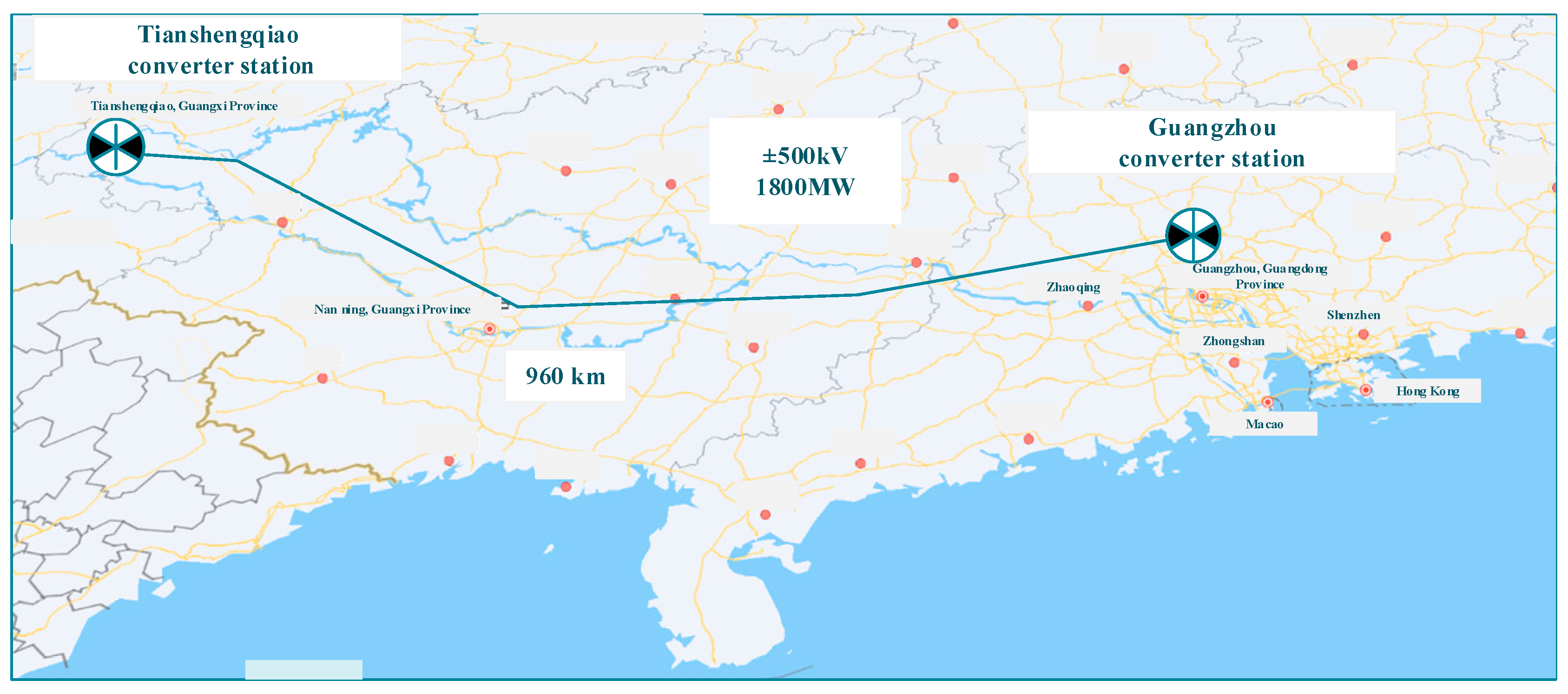
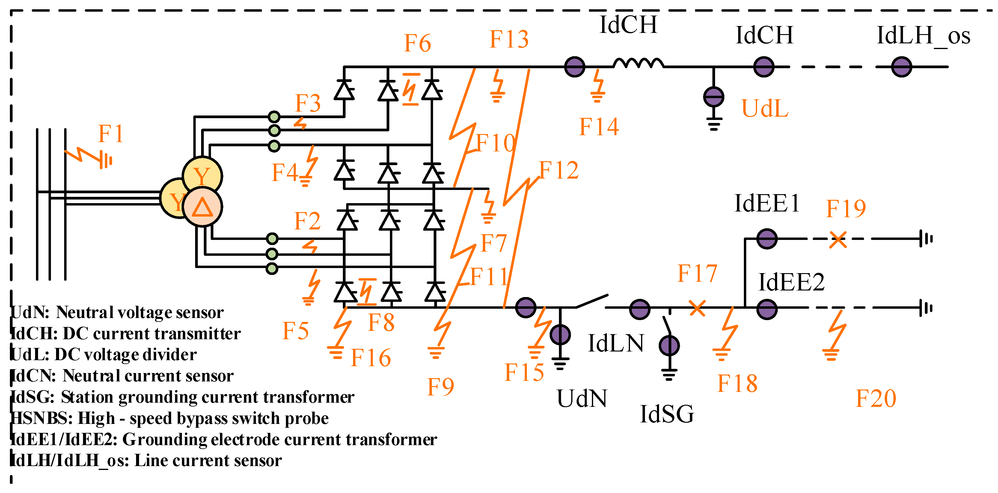
The data used in this study are derived from the measured fault data collected over the past three years from the Tianshengqiao (Guangxi Zhuang Autonomous Region)-Guangzhou (Guangdong Province) HVDC transmission project. Commissioned in 2001, this project serves as a crucial channel for transmitting electrical energy from Southwest China to the load center in South China, with its transmission lines spanning Guangxi Zhuang Autonomous Region and Guangdong Province. The HVDC transmission system of this project has a rated voltage of ±500 kV, a total transmission line length of 960 km, and a rated power of 1800 MW. Figure 2 presents the geographical location map of this HVDC system, Figure 3 illustrates the distribution of main fault points in the substations, and Table 1 details the fault types corresponding to each fault point.
In the actual fault dataset, the overall extraction duration for fault recording data is set to 0.3 s. The fault data includes 15 signal channels that can reflect fault characteristics. The physical meanings corresponding to each signal channel are detailed in Table 2.

2.3.2. Data Augmentation

In the HVDC fault data of this study, the number of samples for AC faults, DC faults, inverter commutation failures, and converter valves are 5, 7, 7, and 9 respectively, indicating a class imbalance problem. This imbalance mainly stems from differences in the actual occurrence probabilities of various faults. To prevent the machine learning algorithm from being biased towards the majority class due to sample imbalance and reduce the recognition accuracy of the minority class faults, this study performs data augmentation on the data. The target number of samples is set to 16 for AC faults, 20 for DC faults, 20 for inverter commutation failures, and 24 for converter valve fault. This setting is intended to simulate the differences in the actual fault probabilities. A diversified noise injection method is adopted for data augmentation. First, the study resamples the samples of fault classes that do not meet the target sample size with replacement. Then, three types of noise (standard Gaussian noise, Laplacian noise, and mixed noise of Gaussian and uniform distributions) are added to the samples exceeding the original number in accordance with a rotation rule. Among them, Laplacian noise is used to simulate impulsive interference, while mixed noise combines the characteristics of the two types of noise to improve the diversity of generated samples. The noise intensity is adaptively set based on the statistical characteristics of the original signal, with the base level set to 0.015 times the standard deviation of the signal. This approach ensures the richness of the samples generated and avoids overfitting.

2.3.3. Data Normalization

In the data preprocessing stage, first, check the integrity and consistency of the data, and remove abnormal sampling points and invalid records. For each type of fault data, concatenate the data from its 15 channels to form a long vector. Then, perform a stacking operation based on the number of samples to construct a comprehensive dataset. Since there are differences in the magnitudes of data from different channels, Z-score standardization is adopted, and its formula is as follows:
x n o r m = X μ σ
where x n o r m represents the standardized data; X is the original data; μ is the mean; and σ is the standard deviation.

3. Fault Diagnosis Model Based on MSF-LightGBM

3.1. Feature Extraction

In this study, two main feature extraction methods were employed to mine more representative and discriminative information from sensor data: sensor-related feature extraction and time-series feature extraction.
(1)
Sensor-related features
This study leverages inter-sensor correlations for fault identification, as correlation features between sensors can reflect the interactions between data from different sensors, which helps capture potential patterns and structures in the data. For instance, the correlation of sensor signals remains stable under normal conditions, while anomalies in the correlation occur under faulty conditions. Therefore, Pearson correlation coefficient is used to measure the linear correlation between sensors. Let the input data matrix be:
X R n × m
where n denotes the number of samples and m denotes the number of features.
It is assumed that the sensor data in each sample can be reshaped into a data matrix with t time steps and s sensors, i.e., t × s = m . In this study, s = 15. For the i-th sample ( i = 1,2 , , n ) , its data is reshaped into a sensor time-series matrix.
S i R t × s
The Pearson correlation coefficient is used to measure the linear correlation between two variables. For sensor j and sensor k  ( j , k = 1,2 , , s ) , their Pearson correlation coefficient is defined as follows:
ρ j k = c o v ( S i : , j , S i : , k ) σ S i : , j σ S i : , k
where c o v ( S i : , j , S i : , k ) denotes the covariance between sensor j and sensor k in the i-th sample, and σ S i : , j and σ S i : , k represent the standard deviations of sensor j and sensor k in the i-th sample, respectively.
By calculating the Pearson correlation coefficients between all pairs of sensors, an s × s correlation coefficient matrix is obtained:
C i R s × s
where C i ( j , k ) = ρ j k .
To reduce the feature dimensionality, this study extracts the upper triangular part of the correlation coefficient matrix. The upper triangular part of the correlation coefficient matrix contains correlation information between all different sensor pairs, thus avoiding redundant calculations. Since faults do not affect the self-correlation of individual sensors, the diagonal elements are not considered as features.
Finally, for each sample i, a correlation feature vector r i with length s ( s 1 ) 2 is obtained. By combining the correlation feature vectors of all samples, a correlation feature matrix is derived:
R R n × s ( s 1 ) 2
(2)
Time-series features
In addition to sensor-related features that capture inter-sensor correlations, time-series features are also extracted to capture the temporal and frequency-domain characteristics of individual samples. The time-series features include statistical features, higher-order statistical features, Fourier transform features, and wavelet transform features.
Statistical features are common indicators that describe the basic distribution characteristics of time-series data, including the mean μ i , the standard deviation σ i , the maximum value M i , the minimum value m i , the quartiles Q i , and the interquartile range I Q R i . The specific formulas are as follows:
μ i = 1 m l = 1 m X i , l
σ i = 1 m l = 1 m ( X i , l μ i ) 2
M i = m a x l = 1 m X i , l
m i = m i n l = 1 m X i , l
Q 1 i = percentile ( X i , 25 )
I Q R i = Q 3 i Q 1 i
where X i , l denotes the l-th feature value of the i-th sample.
Higher-order statistical features include skewness and kurtosis, which are used to describe the distribution shape of time-series data.
Skewness S i measures the degree of asymmetry in the data distribution, and its calculation formula is as follows:
S i = 1 m l = 1 m ( X i , l μ i ) 3 σ i 3
Kurtosis K i measures the degree of peakedness of the data distribution, and its calculation formula is as follows:
K i = 1 m l = 1 m ( X i , l μ i ) 4 σ i 4 3
The Fourier transform can convert time-series data from the time domain to the frequency domain, revealing the frequency components of the data. Discrete fourier transform (DFT) is performed on each sample, and the absolute values of the transformation results are calculated.
For the i-th sample X i , its DFT result is given by:
F i = f f t ( X i )
where f f t denotes the DFT function.
This study calculates the mean μ F i and standard deviation σ F i of the Fourier transform results as the Fourier transform features:
μ F i = 1 m l = 1 m | F i , l |
σ F i = 1 m l = 1 m ( F i , l μ F i ) 2
where F i , l denotes the l-th component of the DFT result of the i-th sample.
The wavelet transform is a multi-resolution analysis method that enables the analysis of time-series data at different scales. This study uses Daubechies wavelets to perform 3-level wavelet decomposition on each sample. For the i-th sample X i , the result of its wavelet decomposition is a set of wavelet coefficients:
W i = [ W i 0 , W i 1 , W i 2 , W i 3 ]
where W i 0 represents the approximation coefficients, and W i 1 , W i 2 , and W i 3 denote the detail coefficients.
Finally, for each sample i, the statistical features, higher-order statistical features, Fourier transform features, and wavelet transform features are combined into a time-series feature vector t i . By combining the time-series feature vectors of all samples, a time-series feature matrix is obtained:
T R n × d
where d is the dimension of the time-series features.

3.2. Feature Selection

After fusing time-series features and sensor-related features, a large number of features are generated. To screen out key features from the fused high-dimensional features, reduce computational costs, and enhance result interpretability, this study performs feature selection on the fused features. Considering that LightGBM is a tree-based model capable of capturing nonlinear interactions between features, RFE filters features based on their importance after these interactions, which is more accurate than univariate filtering. Additionally, RFE is a supervised screening method that relies on labels to determine the contribution of each feature to classification, making it more aligned with the task objective of fault diagnosis compared to unsupervised methods. For these reasons, this study selects RFE as the feature selection method [23].
The principle of RFE is to repeatedly train a model, evaluate feature importance, and eliminate the least important features until a preset number of features are retained. Assuming the initial feature set is denoted as F :
F = { f 1 , f 2 , , f m }
(1)
Initial training
The base model LightGBM is trained using all features in the set F , and the importance of each feature is calculated through the model.
I = { I 1 , I 2 , , I m }
The feature importance of LightGBM is calculated using the gain metric, and the formula is as follows:
I g a i n ( f i ) = s p l i t S i Δ L o s s ( s p l i t )
where S i represents the set of all decision tree split nodes that the feature f participates in, and Δ L o s s ( s p l i t ) denotes the decrease value of the loss function caused by this split.
(2)
Elimination of weak features
Features are sorted by their importance I , and the feature with the lowest importance is eliminated, resulting in a new feature set:
F 1 = F { f m i n ( I ) }
(3)
Recursive iteration
Steps 1–2 are repeated: in each iteration, the model is trained using the current feature set, and the weakest feature is eliminated. This process continues until the size of the feature set reaches k, ultimately resulting in the filtered feature set F f i n a l .

3.3. LightGBM

After conducting data extraction and feature optimization on multi-dimensional operational data, this study selects LightGBM as the classifier, which is characterized by an efficient ensemble learning framework and anti-noise optimization strategies. LightGBM adopts decision trees as base learners and constructs a strong learner through iterative training. Its core mechanism lies in optimizing the current base learner using the loss gradient of the previous round of the model. Eventually, the prediction results of all base learners are integrated to achieve accurate identification of fault types [24]. Assuming that the fault analysis model comprises n base learners H 1 ( x ) , H 2 ( x ) , , H n ( x ) , and the set space of all base learners is denoted as Θ , the output of the final strong learner is the sum of the outputs of all base learners, which is used to determine the fault category.
H n ( x ) = i = 1 n H i ( x ) , H i Θ
where x represents the input sample (fault-related features), and H i ( x ) denotes the classification value of the i-th base learner.
The iterative process follows the logic of gradient descent, with the goal of minimizing the fault diagnosis loss of the current model to train a new base learner. If the strong learner obtained after the first i − 1 iterations is H i 1 ( x ) , its loss function is expressed as:
L ( y , H i 1 ( x ) )
h i ( x ) = arg   m i n h H L y , H i 1 ( x ) + h ( x )
To simplify the optimization of the loss function, LightGBM uses the negative gradient to approximate the residual as the fitting target of the current base learner, which adapts to the deviation correction needs of HVDC fault data. The pseudo-residual is defined as the negative partial derivative of the loss function with respect to the output of the strong learner from the previous iteration:
r i = L y , H i 1 ( x ) H i 1 ( x )
The objective function is typically the squared error, and h i x can be approximately expressed as:
h i x = arg   m i n h H r i h i x 2
Finally, the strong learner for the current iteration is obtained as follows:
H i x = H i 1 x + h i x
In each gradient boosting iteration, the output values of the negative gradient of the current model’s loss function are { g 1 , , g n } , where g i represents the value of the negative gradient of the loss function corresponding to x i at the output of the current model. The base learner performs splitting at the feature split point with the maximum information gain, and the information gain is measured by the variance after splitting.
LightGBM adopts a leaf-wise growth approach for decision tree splitting. Let O denote the dataset within a fixed node of the base model. The variance gain of the feature at split point d for this node j is defined as:
V j | O d = 1 n O x i O : x i j d g i 2 n l | O j d + x i O : x i j d g i 2 n r | O j d
where n O denotes the number of training set samples in a specific fixed leaf node; n l | O j d represents the number of samples in the j-th feature with values ≤ d; and n r | O j d is the number of samples in the j-th feature with values > d. By iterating through each split point of every feature, the corresponding feature d j = arg   m a x V j ( d ) is identified, and the maximum information gain V j d j for this feature is calculated. The data is then divided into left and right child nodes based on the split point d j .

3.4. MSF-LightGBM

The MSF-LightGBM fault diagnosis algorithm is a multi-modal feature fusion classification algorithm designed for fault diagnosis of HVDC systems.
First, a structured data loading module is designed to read original fault event files, extract time-series data from 15 key signal channels and flatten the two-dimensional time-series data into one-dimensional initial sample vectors, laying a solid data foundation for subsequent processing.
Secondly, to address the prevalent issue of unbalanced sample distribution in HVDC fault diagnosis, an intelligent balanced augmentation strategy is proposed. Based on the preset target sample distribution for the four types of faults, the strategy first expands the sample size through resampling and then injects three types of rotational noise into the augmented samples. This design not only balances the sample quantity of each fault category but also simulates signal interference in actual operating conditions, significantly enhancing the model’s robustness to environmental noise in engineering applications.
Thirdly, the core multi-modal feature extraction stage is implemented, consisting of two key modules: (1) Sensor correlation feature extraction: For each sample, the flattened one-dimensional data is reconstructed into a two-dimensional time-series matrix to restore the temporal correlation between sensors; Pearson correlation coefficients are calculated for all pairs of the 15 sensors to construct a 15 × 15 correlation matrix; to avoid information redundancy of the symmetric matrix, only the upper triangular elements (excluding the diagonal) are extracted as correlation features, ultimately forming a 105-dimensional feature vector that effectively captures the inter-sensor collaborative characteristics of faults. (2) Time-series feature extraction: A four-level hierarchical feature set is constructed to comprehensively capture the time-domain, frequency-domain, and time-frequency domain characteristics of fault signals, enabling in-depth mining of fault information.
Subsequently, the 105-dimensional sensor correlation features and 21-dimensional time-series features are fused to form a 126-dimensional multi-modal feature set. To eliminate redundant information and reduce computational complexity, the RFE algorithm is adopted-with the LightGBM classifier as the evaluation criterion-to screen out 15 most discriminative key features from the fused feature set, effectively avoiding overfitting caused by high-dimensional data.
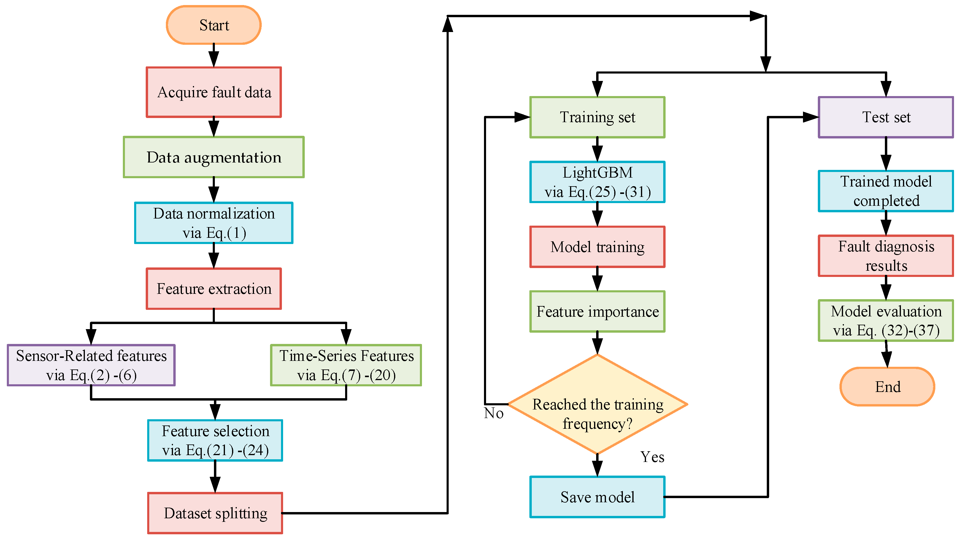
Finally, the dataset is fixedly divided into a training set and a test set at a ratio of 7:3 based on faulty events. Based on balanced samples and screened key features, the LightGBM classifier is adopted for model training. This classifier gives full play to its advantages in parallel computing and multi-classification, achieving accurate identification of the four types of HVDC faults. The flow chart of the MSF-LightGBM algorithm is shown in Figure 4.

4. Case Study

4.1. Experimental Environment Configuration

In this paper, a comprehensive comparative experiment is designed to verify the effectiveness of the proposed HVDC fault diagnosis method based on MSF-LightGBM. The experiment is conducted on a computer equipped with an Intel(R) Core (TM) i5-14600K processor with a main frequency of 3.50 GHz and 64.0 GB of RAM. The operating system is the 64-bit Windows 11 Professional Edition. The development environment is built on Python 3.9 (PyCharm Community Edition 2024), with key dependent libraries and their versions specified as follows: NumPy 1.24.3, Pandas 2.0.3, Scikit-learn 1.2.2, LightGBM 3.3.5, PyWavelets 1.4.1, Matplotlib 3.7.1, and Seaborn 0.12.2. These libraries provide support for data processing, feature engineering, model training, and visualization.

4.2. Experimental Settings

To objectively evaluate the performance advantages of the HVDC fault diagnosis model proposed in this study, seven classic algorithms are selected as comparison methods, including: Multimodal [25], which fuses time-series features and image features—specifically, it employs the Gramian angular field (GAF) to convert one-dimensional time-series signals into two-dimensional images with a specified image size (32 × 32), and the “summation” method, which utilizes a CNN model with two convolutional layers and two fully connected layers to extract discriminative features from GAF images while extracting time-series features including statistical features, higher-order statistical features, frequency-domain features, and time-frequency features, and finally adopts the LightGBM classifier for fault classification-along with LSTM [26], support vector machine (SVM) [27], K-nearest neighbors (KNN) [28], random forest (RF) [29], LightGBM [30], and one-dimensional convolutional neural network (1D-CNN) [31]. The specific parameter configurations of all algorithms are detailed in Table 3.
In terms of model performance evaluation, considering the data class imbalance in the actual fault diagnosis scenario, this paper adopts five main indicators, namely precision, accuracy, recall, F1-score and Balanced Accuracy, for comprehensive evaluation [32]. The formulas for the evaluation indicators are as follows:
P r e c i s i o n = T P T P + F P
A c c u r a c y = T P + T N T P + T N + F P + F N
R e c a l l = T P T P + F N
F 1 = 2 × P r e c i s i o n × R e c a l l P r e c i s i o n + R e c a l l
B a l a n c e d   A c c u r a c y = R e c a l l + T N R 2
T N R = T N T N + F P
where true positive (TP) refers to the number of samples that are actually positive and predicted as positive by the model; false positive (FP) refers to the number of samples that are actually negative but predicted as positive by the model; true negative (TN) refers to the number of samples that are actually negative and predicted as negative by the model; false negative (FN) refers to the number of samples that are actually positive but predicted as negative by the model.

4.3. Comparative Experiment

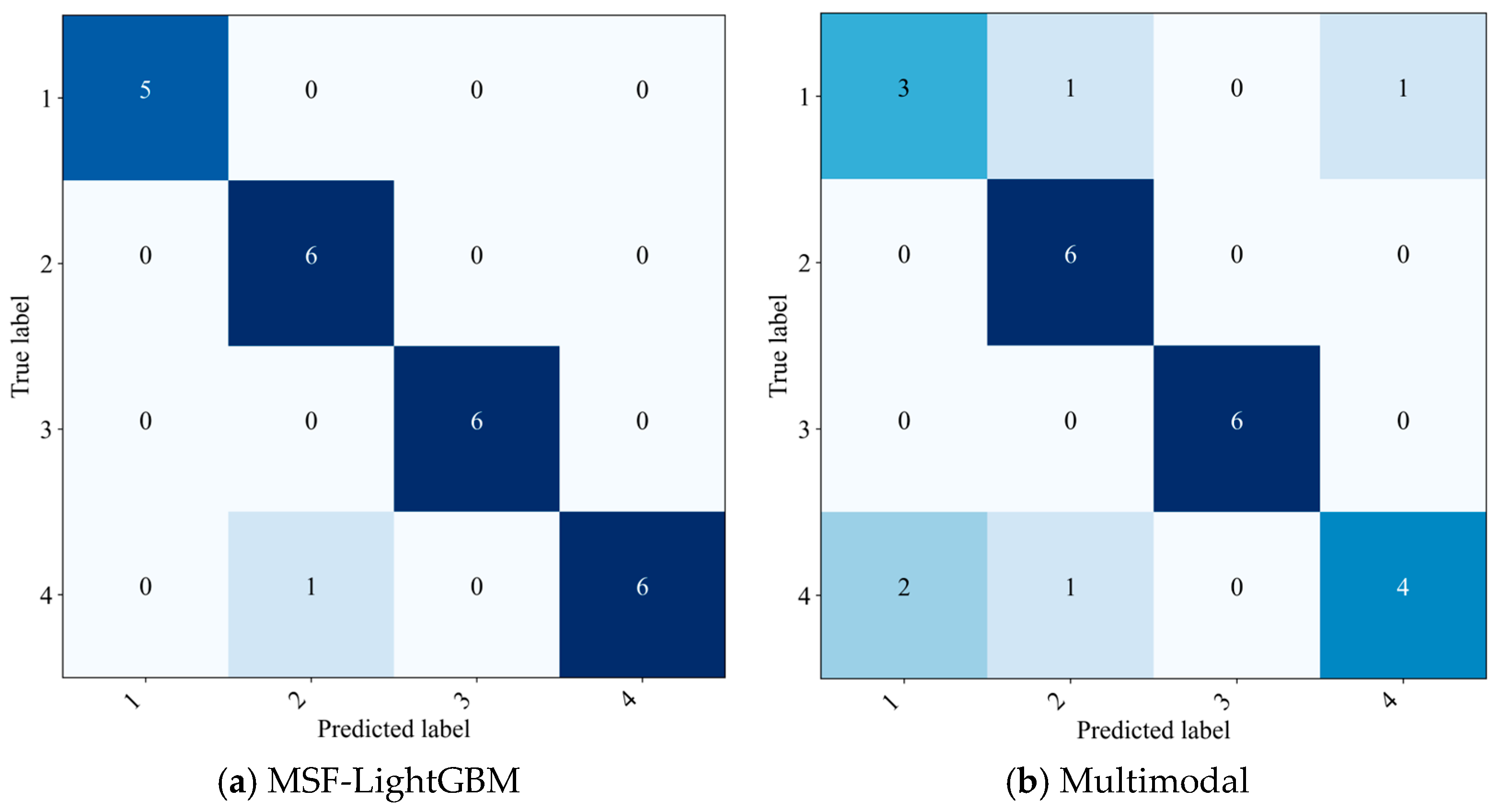
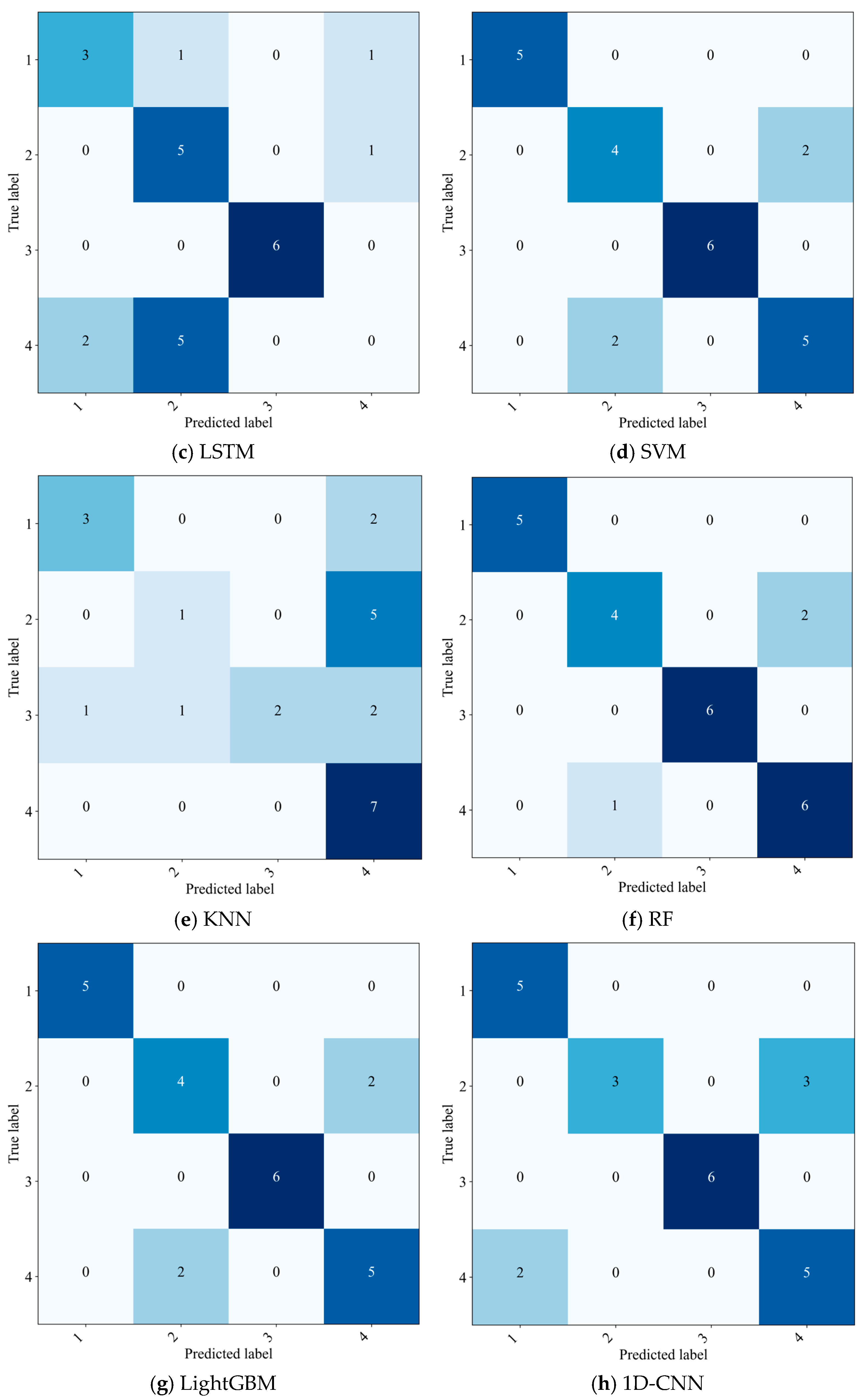
This study uses the confusion matrix to evaluate the performance of eight different methods in HVDC fault diagnosis. In the confusion matrix, the horizontal axis represents the predicted labels, and the vertical axis represents the true labels. There are specifically four types of fault labels: Label 1 represents AC faults, Label 2 represents DC faults, Label 3 represents converter valve faults, and Label 4 represents inverter commutation failures. The relevant diagnostic results are shown in Figure 5.
In Figure 5a, the predicted results are largely clustered along the main diagonal, indicating that the predicted labels are roughly in one-to-one correspondence with the true labels. By contrast, the LightGBM algorithm in Figure 5g still exhibits significant limitations in the diagnosis of DC faults and inverter commutation failures. This comparison fully confirms the effectiveness of the multimodal sensor-feature fusion strategy in HVDC fault diagnosis. The confusion matrix of the LSTM method in Figure 5c is remarkably scattered; the counts on the diagonal for true labels 1 and 4 are zero, demonstrating its inability to correctly identify AC faults and inverter commutation failures, and thus yielding the worst performance. This limitation can be attributed to the insufficient discriminative power of temporal features alone for separating different fault classes. A further comparison with the Multimodal approach (Figure 5b), which combines temporal and image features, shows that most predictions also cluster along the main diagonal, corroborating that image features supply complementary information that boost diagnostic accuracy. Nevertheless, the increment is modest, suggesting that the fusion scheme itself warrants deeper investigation to fully exploit the potential of multimodal data in this context. The remaining four benchmark algorithms deliver intermediate performance; occasional misclassifications still occur, e.g., in Figure 5d the SVM confuses two DC faults with inverter commutation failures.
Table 4 presents the quantitative analysis results of the performance in HVDC fault diagnosis, including 5 indicators, e.g., precision, accuracy, recall, F1-score and balanced accuracy. It can be clearly observed from the table that MSF-LightGBM performs the best among the eight algorithms, with a Balanced Accuracy as high as 0.9752. Compared with the other seven algorithms, this model demonstrates superior performance across all evaluation metrics. The F1-score, which provides a harmonic measure of precision and recall, offers a comprehensive assessment of the model’s diagnostic capability. Among the comparison algorithms, RF has a relatively high F1-score. However, the F1-score of MSF-LightGBM exhibits a more substantial F1-score, outperforming RF by 0.0797. This significant increase indicates a concurrent enhancement in both precision and recall. Furthermore, balanced accuracy is a critical metric for evaluating performance on imbalanced datasets, a common characteristic of real-world fault data. While RF performs prominently in terms of balanced accuracy, the MSF-LightGBM model achieves a further improvement of 0.0564. These results confirm that the combination of multi-modal sensor features fusion and the lightweight gradient boosting machine enables MSF-LightGBM to fully explore and utilize various types of data features. Consequently, the proposed method significantly improves the accuracy and stability of multi-class fault diagnosis and maintains robust performance when applied to imbalanced data distribution.
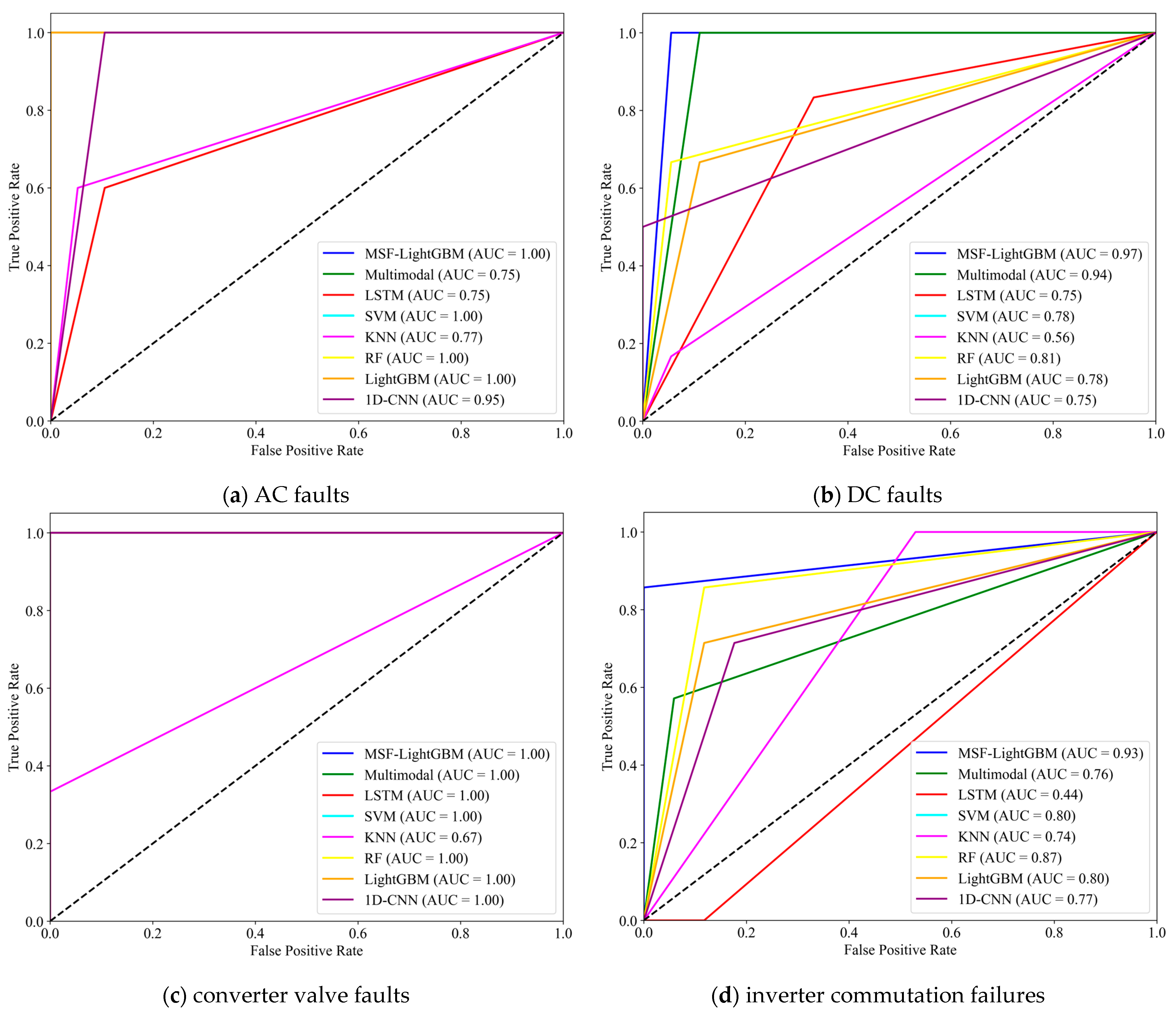
The diagnostic performance of the six algorithms for the four types of faults was quantitatively compared using ROC curves. In an ROC curve, the false positive rate (FPR), plotted on the horizontal axis, represents the probability of a false alarm. The true positive rate (TPR), plotted on the vertical axis, indicates the model’s ability to correctly identify faults. A diagonal “line of no-discrimination” (slope = 1) serves as a performance baseline, indicating random guessing. A curve approaching this line suggests a diagnostically useless classifier. Conversely, a curve that shifts toward the upper-left corner signifies an optimal balance between a high TPR and a low FPR, reflecting superior diagnostic performance. As shown in Figure 6, the proposed MSF-LightGBM model demonstrates a curve closest to the ideal point (0,1), significantly outperforming the benchmark models.
Based on the quantitative analysis of the ROC curves in Figure 6, the proposed MSF-LightGBM algorithm demonstrates superior diagnostic capability across all four fault types. Its ROC curve is consistently positioned closest to the upper-left corner, with the area under the curve (AUC) achieving a perfect value of 1.0 for AC faults and converter valve faults. This proves that the algorithm possesses optimal and stable diagnostic performance.
In contrast, the diagnostic adaptability of the other seven algorithms varies significantly with fault types: the LightGBM algorithm performs relatively well in the diagnosis of AC faults, while the Multimodal algorithm exhibits superior diagnostic performance for DC faults. For converter valve faults, all seven algorithms except KNN achieve satisfactory performance, with their ROC curves clustered near the upper-left corner. Whereas, in the diagnosis of inverter commutation failures, the RF algorithm demonstrates the most prominent performance advantage among all benchmark models.

4.4. Ablation Experiment

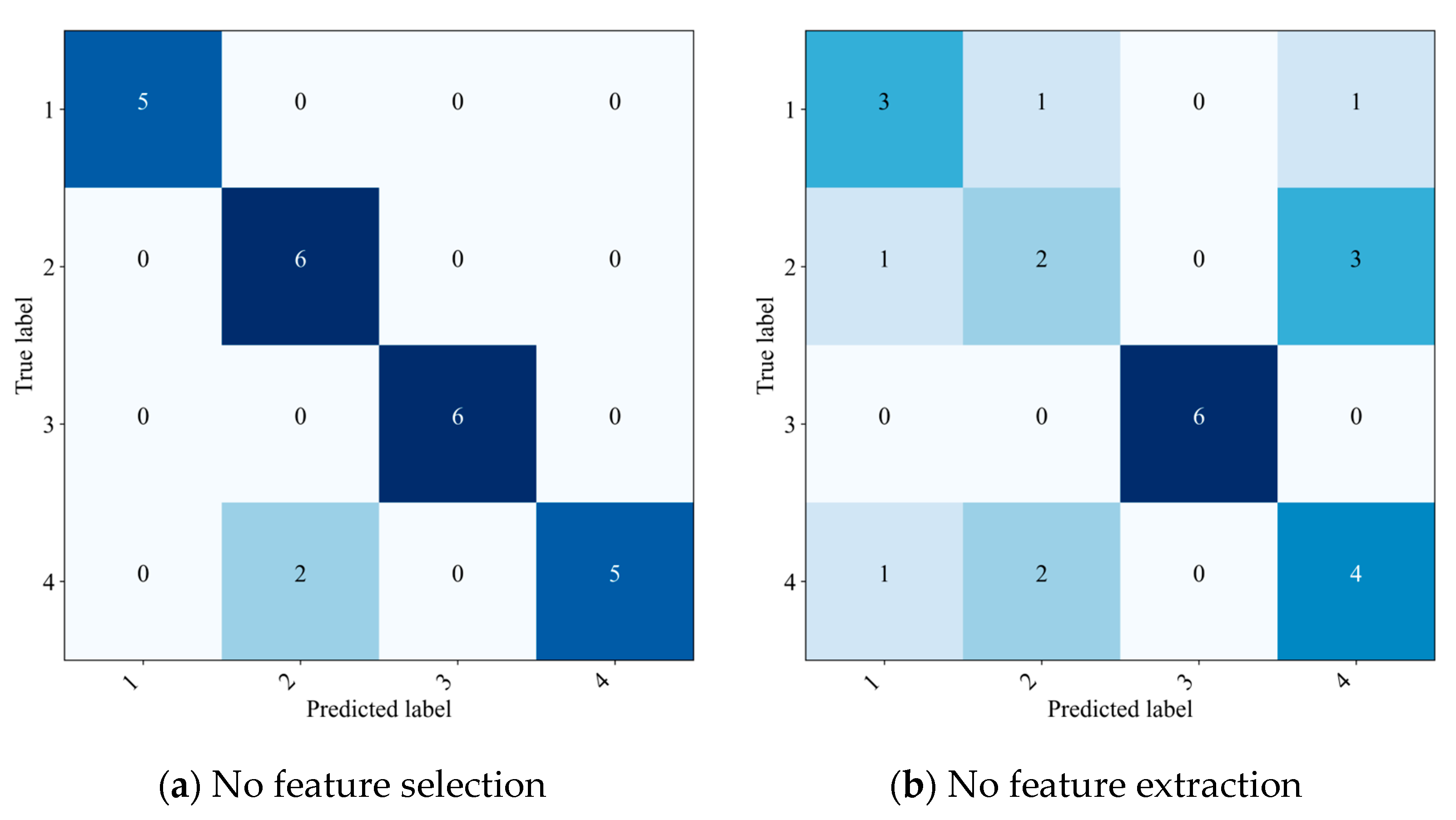
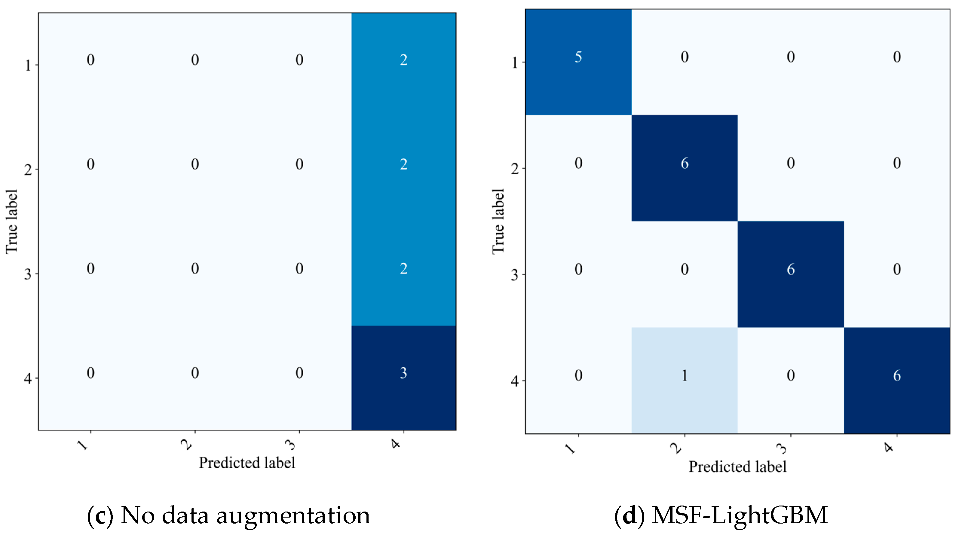
To deeply explore how feature selection, feature extraction, and data augmentation affect the model’s overall performance and unveil its internal working principles, this study conducted an ablation experiment on MSF-LightGBM. During the experiment, specific components of the model were removed in a controlled manner to systematically evaluate the effects of each component on the model’s performance. The results of the ablation experiment are presented in detail in Table 5 and Figure 7.
According to the results presented in Table 5 and Figure 7, data augmentation, feature extraction and feature selection all exert varying degrees of influence on the performance of the MSF-LightGBM model. Among these, data augmentation has the most significant impact. When data augmentation is not applied, the model’s F1-score drops substantially to 0.125, and the balanced accuracy decreases to 0.5. As can be observed from Figure 7c, the confusion matrix reveals that the prediction outcomes exhibit severe randomness, indicating the model’s inability to effectively distinguish between different classes. This is attributed to the relatively small dataset size prior to augmentation, which makes the model prone to overfitting. With limited data, the model struggles to accurately estimate the true data distribution. Statistical features are not prominent, and the model fails to cover all possible feature combinations and variations. Consequently, it learns only localized and non-representative feature patterns, severely compromising both performance and generalization capability. Feature extraction also plays a crucial role in model performance. Without feature extraction, the model’s F1-score decreases to 0.6242, and the balanced accuracy drops to 0.7497. It can be seen from Figure 7b that although the overall model performance remains acceptable, significant confusion occurs between certain classes, such as misclassifying DC faults as inverter commutation failures. This demonstrates that the Multimodal Sensor Feature Fusion method proposed in this study effectively enhances the model’s capability to capture discriminative data features. Similarly, feature selection has a notable influence on the model. In the absence of feature selection, multiple performance metrics decline: the F1-score decreases from 0.9615 to 0.9226, and the balanced accuracy drops from 0.9752 to 0.9504. The confusion matrix in Figure 7a shows sporadic misclassifications and the presence of a small number of false positive samples. This indicates that feature selection helps identify key features with greater impact on model performance, eliminates redundant and irrelevant features, and thereby improves both model accuracy and generalization ability.

4.5. Sensitivity Analysis

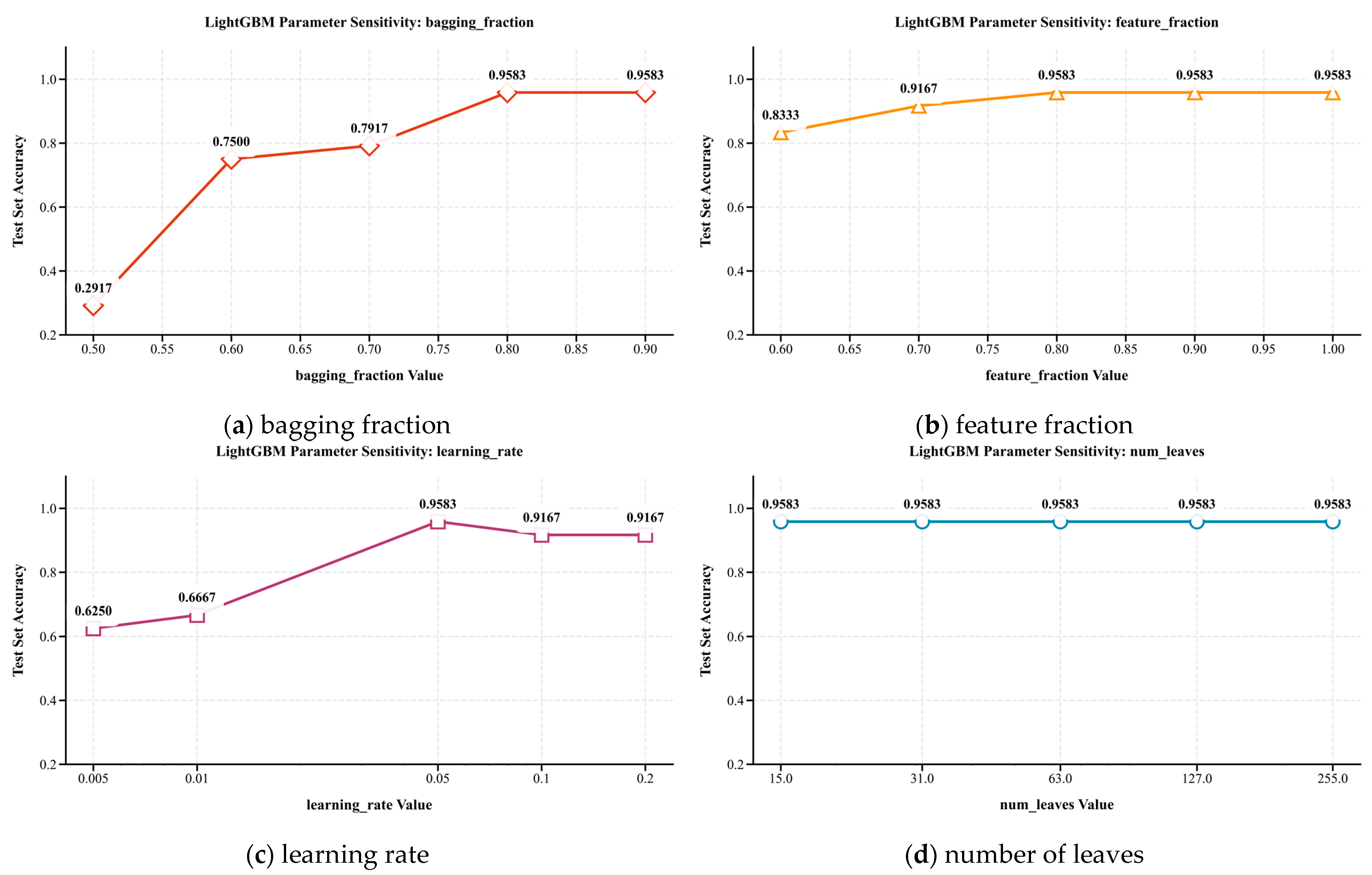
In the construction and optimization of machine learning models, model parameter selection is crucial, as it directly affects the model’s performance and generalization performance. Sensitivity analysis can quantify the impact of each parameter on the model’s performance, which helps us understand the relationship between parameters and performance and provides a scientific basis for parameter optimization and adjustment to maximize the model’s performance. In this study, a sensitivity analysis was conducted on four main parameters of the MSF-LightGBM algorithm, namely number of leaves, learning rate, feature fraction, and bagging fraction. By systematically changing the values of these parameters and observing the changes in the model’s accuracy, the sensitivity of each parameter was evaluated. The specific results are shown in Figure 8.
According to the sensitivity analysis results of the four main parameters in Figure 8, bagging fraction controls the proportion of data used for training each tree. When it takes a relatively small value of 0.5, the model’s accuracy is only 0.29, indicating that the model fails to fully utilize the data. When it increases to 0.8, the accuracy rapidly reaches 0.9583 and remains stable. This suggests that an appropriate bagging fraction can improve the model’s performance. Although a larger bagging fraction also leads to higher accuracy, it increases the computational cost. Learning rate determines the step size of the model update in each iteration. When its value is 0.005, the model’s accuracy is 0.625, which is not satisfactory. When it increases to 0.05, the accuracy reaches 0.9583 and remains stable, indicating that an appropriate learning rate can accelerate the convergence of the model and improve the accuracy. In contrast, the number of leaves and feature fraction have a minimal impact on the model’s accuracy. When the feature fraction is 0.6, the accuracy is 0.8333, and when it reaches 0.8, the accuracy rises to 0.9583 and then remains stable. Meanwhile, the model’s accuracy consistently stays at 1.0 regardless of changes in the number of leaves. This indicates that under the current dataset and model architecture, tree complexity (determined by the number of leaves) and the degree of feature utilization (governed by the feature fraction) have limited effects on the model’s performance. Based on the experimental results, the parameter optimization recommendations are as follows: set the bagging fraction to 0.7, the learning rate to 0.05, and the feature fraction to 0.9; the number of leaves can be flexibly selected within a reasonable range.

4.6. Analysis of Feature Importances

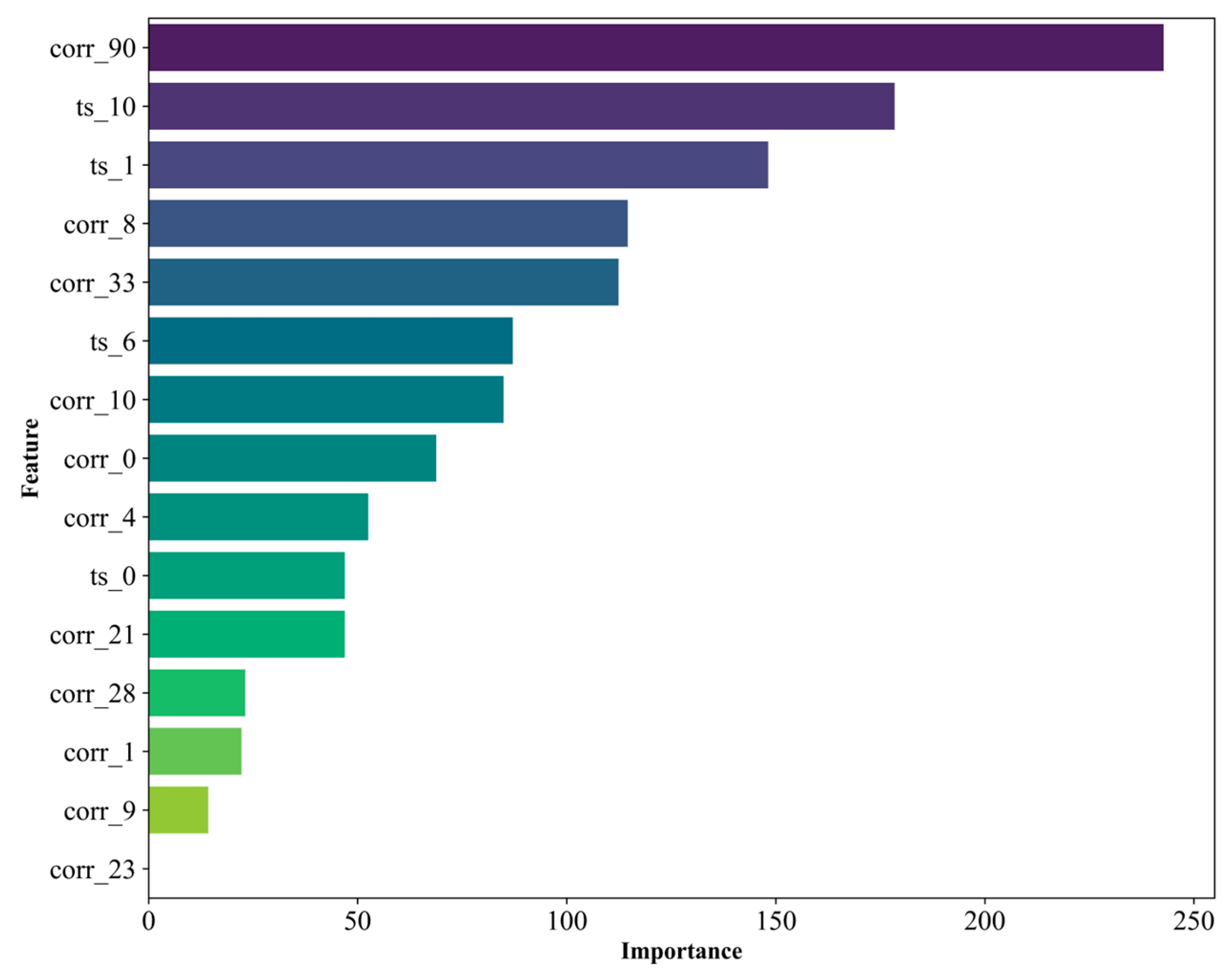
To verify the laws of HVDC physical characteristics and the reliability of the model, this paper conducts a feature importance analysis, and the feature importance results are shown in Figure 9. The top five important features are as follows: The correlation between the extinction angle and the turn-off angle (corr_90), which reflects the synergistic variation of key angle parameters during the commutation process of the HVDC converter, consistent with the physical logic of commutation; The standard deviation of the Fast Fourier Transform (FFT) (ts_10), which captures the harmonic fluctuation characteristics during faults (since harmonic components are important indicators of HVDC faults); The standard deviation of the signal (ts_1), a statistical feature quantifying signal fluctuation that increases significantly during faults; The correlation between converter voltage and turn-off angle (corr_8), which links the electrical quantity of the converter with its commutation state, and is physically meaningful for identifying converter faults; and The correlation between valve-side voltage and turn-off angle (corr_33), which reflects the physical connection between valve-side electrical quantity and commutation angle, and its variation during faults is a reasonable physical indicator. The feature importance analysis verifies the consistency between these features and the physical characteristics of the HVDC system, enhancing the interpretability and credibility of the model.

4.7. Leave-One-(Original)-Event Cross-Validation

In this study, the original dataset has an extremely small sample size. To simulate a generalization scenario closer to engineering practice, the leave-one-(original)-event cross-validation is adopted. This cross-validation strategy uses all augmented samples of N − 1 original fault events for training and retains all augmented samples of only one original event for testing. The test results are shown in Table 6. The table contains the test results of 28 groups of original fault events, and the average accuracy of all test events is 0.821, indicating that the method performs well overall in the cross-original-event generalization test. Although the accuracy of individual events (such as AC faults_5, inverter commutation failures_1, and inverter commutation failures_2, etc.) is lower than 1.0, most events can still achieve accurate recognition. Despite the extremely small scale of the original dataset, through the combination of data augmentation technology and leave-one-(original)-event cross-validation, the proposed method demonstrates good performance in the generalization test of various fault events. It can effectively deal with unknown fault scenarios at the original event level, fully verifying the applicability of the method in small sample augmented scenarios.

5. Conclusions and Future Work

This study addresses the issues of sample imbalance, insufficient feature mining, and low diagnostic accuracy in HVDC system fault diagnosis. A fault diagnosis model based on MSF-LightGBM is proposed. Through experimental verification and analysis, the following conclusions are drawn:
(1)
A data augmentation method with multi-type noise injection is adopted to adjust the sample size of each fault category to the target distribution. This resolves the model bias problem caused by minority-class faults in the original data, and the model’s Balanced Accuracy for minority-class faults increases from 0.5 to 0.9752.
(2)
By fusing time-series features and sensor correlation features, a comprehensive feature vector is constructed to capture the instantaneous mutation, frequency-domain distribution, and inter-sensor collaborative change information of fault signals. Compared with single-modal feature input for LightGBM, the F1-score has improved from 0.8452 to 0.9615. The multi-modal feature fusion enables the model to reveal the intrinsic physical characteristics of different HVDC faults, which helps field operators quickly locate fault sources. This shortens the fault recovery time, reduces economic losses caused by system downtime, and improves the availability of the HVDC transmission system.
(3)
Feature selection is carried out through RFE to screen out key features, reducing the interference of redundant features. Combined with the efficient classification capability of LightGBM, the model’s accuracy, recall, and F1-score on the test set all reach above 0.95, and the average AUC value of the four ROC curves is 0.975, which is significantly superior to traditional algorithms.
(4)
From the perspective of engineering application, the MSF-LightGBM model integrates data balance, multi-modal feature mining, and efficient classification into a modular framework, which is easy to implement and promote in actual HVDC control systems. Its high diagnostic accuracy helps reduce the dependence on manual experience in fault diagnosis, standardize the fault handling process, and lower the operation and maintenance costs of HVDC projects. This provides a reliable technical solution for the intelligent development of power grids and supports the stable operation of long-distance, large-capacity HVDC transmission systems.
However, this study still has three limitations: First, it does not consider composite faults under extreme operating conditions, and the types of fault samples need to be further expanded; Second, the experimental data of this study have specificity, and the adaptability of the model in other environments still needs to be verified; Third, the number of original data samples is relatively small, and the issue of information leakage has not been fully considered during data augmentation.
Corresponding to the above limitations and engineering practical requirements, future research can be carried out in the following three aspects:
(1)
Construct a mixed sample library containing both single faults and composite faults to address the problem of multi-fault superposition;
(2)
Validate the proposed model on completely independent HVDC systems from different projects or operators, with a focus on enhancing its cross-system generalization capability and robustness;
(3)
To address the issue of information leakage, data augmentation should be performed after splitting the training and test sets. Specifically, only the training set is augmented, while the original data are retained for the test set, thereby ensuring the authenticity of the experiment.

Author Contributions

Q.L.: writing—original draft preparation; Y.L.: methodology; S.Z.: data curation and visualization; Y.M.: software and formal analysis; Y.Q.: software and formal analysis; X.L.: conceptualization; B.Y.: writing—review and editing. All authors have read and agreed to the published version of the manuscript.

Funding

This research was funded by the National Natural Science Foundation of China (62263014) and the Research on Key Technologies of DC Transmission Operation and Maintenance Knowledge Iteration and Intelligent Decision-Making Based on Multimodal Generative Pre-Trained Models-Topic 2: Research on DC Transmission Operation and Maintenance Intelligent Decision-Making Technology Based on Multimodal Pre-trained Models (CGYKJXM20240120).

Data Availability Statement

The original contributions presented in the study are included in the article, further inquiries can be directed to the corresponding author.

Conflicts of Interest

Authors Qiang Li, Yingfei Li, Shihong Zhang, Yue Ma, Yinan Qiu, Xiaohang Luo were employed by the company EHV Power Transmission Company of China Southern Power Grid Co., Ltd. The remaining author declare that they have no known competing financial interests or personal relationships that could have appeared to influence the work reported in this paper.

Nomenclature

Abbreviations
AUCarea under the curve
ACalternating current
BPback propagation
BiGRUbidirectional gated recurrent unit
CatBoostcategorical boosting
CEEMDANcomplete ensemble empirical mode decomposition with adaptive noise
CNNconvolutional neural network
DCdirect current
DFTdiscrete fourier transform
DWTdiscrete wavelet transform
FNfalse negative
FPfalse positive
FPRfalse positive rate
GAFgramian angular field
HVDChigh-voltage direct current
KNNK-nearest neighbors
LightGBMlight gradient boosting machine
MSF-LightGBMmultimodal sensor feature-light gradient boosting machine
PCAprincipal component analysis
RFrandom forest
RFErecursive feature elimination
ROCreceiver operating characteristic
SVMsupport vector machine
TNtrue negative
TPtrue positive
TPRtrue positive rate
WPTwavelet packet transform
1D-CNNone-dimensional convolutional neural network
Variables
c o v ( S i : , j , S i : , k ) covariance between sensor j and sensor k in the i-th sample
d dimension of the time-series features
f f t DFT function
F i , l the l-th component of the DFT result of the i-th sample
F P number of samples that are actually negative but predicted as positive by the model
F N number of samples that are actually positive but predicted as negative by the model
H i ( x ) classification value of the i-th base learner
m number of features
n number of samples
n O number of training set samples in a specific fixed leaf node
n l | O j d standard deviation of the data.
n r | O j d constants to prevent division by zero errors
S i set of all decision tree split nodes
TPnumber of samples that are actually positive and predicted as positive by the model
TNnumber of samples that are actually negative and predicted as negative by the model
W i 0 approximation coefficients
W i 1 detail coefficients
x n o r m standardized data
X original data
X i , l the l-th feature value of the i-th sample
x input sample
μ mean
σ standard deviation
σ S i : , j standard deviations of sensor j in the i-th sample
σ S i : , k standard deviations of sensor k in the i-th sample
Δ L o s s ( s p l i t ) decrease value of the loss function caused by this split

References

  1. Han, J.Y.; Wang, J.X.; He, Z.H.; An, Q.; Song, Y.Y.; Mujeeb, A.; Tan, C.W.; Gao, F. Hydrogen-powered smart grid resilience. Energy Convers. Econ. 2023, 4, 89–104. [Google Scholar] [CrossRef]
  2. Zhang, W.Z.; Xu, C.B. Capacity configuration optimization of photovoltaic-battery-electrolysis hybrid system for hydrogen generation considering dynamic efficiency and cost learning. Energy Convers. Econ. 2024, 5, 78–92. [Google Scholar] [CrossRef]
  3. Chen, X.P.; Wang, L.; Jiang, Y.N.; Wang, J.X. A peer-to-peer joint energy and reserve market considering renewable generation uncertainty: A generalized Nash equilibrium approach. Energy Convers. Econ. 2024, 5, 179–192. [Google Scholar] [CrossRef]
  4. Wang, J.B.; Wen, J.F.; Wang, J.R.; Yang, B.; Jiang, L. Water electrolyzer operation scheduling for green hydrogen production: A review. Renew. Sustain. Energy Rev. 2024, 203, 114779. [Google Scholar] [CrossRef]
  5. Hassan, S.J.U.; Mehdi, A.; Haider, Z.; Song, J.S.; Abraham, A.D.; Shin, G.S.; Kim, C.H. Towards medium voltage hybrid AC/DC distribution systems: Architectural Topologies, planning and operation. Int. J. Electr. Power Energy Syst. 2024, 159, 110003. [Google Scholar] [CrossRef]
  6. Guo, H.L.; Zhang, Z.R.; Xu, Z. Parallel converter-based hybrid HVDC System for integration and delivery of large-scale renewable energy. J. Mod. Power Syst. Clean Energy 2025, 13, 688–697. [Google Scholar] [CrossRef]
  7. Zhang, T.; Yao, J.; Lin, Y.C.; Jin, R.Y.; Zhao, L.S. Impact of control interaction of wind farm with MMC-HVDC transmission system on distance protection adaptability under symmetric fault. Prot. Control Mod. Power Syst. 2025, 10, 83–101. [Google Scholar] [CrossRef]
  8. Shafique, G.; Boukhenfouf, J.; Gruson, F.; Colas, F.; Guillaud, X. DC voltage control with grid-forming capability for enhancing stability of HVDC system. J. Mod. Power Syst. Clean Energy 2025, 13, 66–78. [Google Scholar] [CrossRef]
  9. Su, C.S.; Yin, C.Y.; Li, F.T.; Han, L. A Novel Recovery Strategy to Suppress Subsequent Commutation Failure in an LCC-Based HVDC. Prot. Control Mod. Power Syst. 2024, 9, 38–51. [Google Scholar] [CrossRef]
  10. Farkhani, J.S.; Çelik, Ö.; Ma, K.; Bak, C.L.; Chen, Z. Fault detection, classification, and location based on empirical wavelet transform-teager energy operator and ANN for hybrid transmission lines in VSC-HVDC systems. J. Mod. Power Syst. Clean Energy 2025, 13, 840–851. [Google Scholar] [CrossRef]
  11. Li, X.Y.; Wu, X.D.; Wang, T.Y.; Xie, Y.N.; Chu, F.L. Fault diagnosis method for imbalanced data based on adaptive diffusion models and generative adversarial networks. Eng. Appl. Artif. Intell. 2025, 147, 110410. [Google Scholar] [CrossRef]
  12. Li, T.; Li, Y.L.; Chen, X.L. Fault Diagnosis with wavelet packet transform and principal component analysis for multi-terminal hybrid HVDC network. J. Mod. Power Syst. Clean Energy 2021, 9, 1312–1326. [Google Scholar] [CrossRef]
  13. Liang, Y.; Zhang, J.W.; Shi, Z.; Zhao, H.B.; Wang, Y.; Xing, Y.H.; Zhang, X.W.; Wang, Y.J.; Zhu, H.X. A fault identification method of hybrid HVDC system based on wavelet packet energy spectrum and CNN. Electronics 2024, 13, 2788. [Google Scholar] [CrossRef]
  14. Wang, Y.T.; Zheng, D.K.; Jia, R. Fault diagnosis method for MMC-HVDC based on Bi-GRU neural network. Energies 2022, 15, 994. [Google Scholar] [CrossRef]
  15. Yousaf, M.Z.; Liu, H.; Mustafa, A. Deep learning-based robust DC fault protection scheme for meshed HVDC grids. CSEE J. Power Energy Syst. 2023, 9, 2423–2434. [Google Scholar] [CrossRef]
  16. Cao, R.R.; Yang, T.G.; Li, G.H.; Chen, S.L. Diagnosis of commutation failure in a high voltage direct current transmission system based on fuzzy entropy feature vectors and a PCNN-GRU. IEEE Access 2025, 13, 110709–110724. [Google Scholar] [CrossRef]
  17. Wu, J.Y.; Li, Q.; Chen, Q.; Zhang, N.; Mao, C.Z.; Yang, L.T.; Wang, J.Y. Fault diagnosis of the HVDC system based on the CatBoost algorithm using knowledge graphs. Front. Energy Res. 2023, 11, 1144785. [Google Scholar] [CrossRef]
  18. Zheng, R.N.; Hu, Z.S.; Wen, Z.X.; Wang, J.J. AC fault detection method for HVDC system. Guangdong Electr. Power 2020, 33, 97–104. (In Chinese) [Google Scholar]
  19. Lin, S.; Mu, D.L.; Liu, L.; Lei, Y.Q.; Dong, X.Z. A novel fault diagnosis method for DC filter in HVDC systems based on parameter identification. IEEE Trans. Instrum. Meas. 2020, 69, 5969–5971. [Google Scholar] [CrossRef]
  20. Liu, C.C.; Zhou, F.; Wang, F. Fault diagnosis of commutation failure using wavelet transform and wavelet neural network in HVDC transmission system. IEEE Trans. Instrum. Meas. 2021, 70, 3525408. [Google Scholar] [CrossRef]
  21. Li, Q.; Chen, Q.; Wu, J.Y.; Qiu, T.Q.; Zhang, C.H.; Huang, Y.L.; Guo, J.B.; Yang, B. XGBoost-based intelligent decision making of HVDC system with knowledge graph. Energies 2023, 16, 2405. [Google Scholar] [CrossRef]
  22. Chen, Q.; Li, Q.; Wu, J.; He, J.; Mao, C.; Li, Z.; Yang, B. State Monitoring and Fault Diagnosis of HVDC System via KNN Algorithm with Knowledge Graph: A Practical China Power Grid Case. Sustainability 2023, 15, 3717. [Google Scholar] [CrossRef]
  23. Wu, Z.L.; Fan, X.Y.; Bian, G.B.; Liu, Y.H.; Zhang, X.K.; Chen, Y.Q. Short-term wind power forecast with turning weather based on DBSCAN-RFE-LightGBM. Renew. Energy 2025, 251, 123217. [Google Scholar] [CrossRef]
  24. Lu, Z.Y.; Wang, L.S.; Wang, P.B. Microgrid fault detection method based on lightweight gradient boosting machine–neural network combined modeling. Energies 2024, 17, 2699. [Google Scholar] [CrossRef]
  25. Huang, Y.F.; Tao, J.; Zhao, J.Y.; Sun, G.; Yin, K.; Zhai, J.Y. Graph structure embedded with physical constraints-based information fusion network for interpretable fault diagnosis of aero-engine. Energy 2023, 283, 129120. [Google Scholar] [CrossRef]
  26. Lim, J.S.; Cho, H.; Kwon, D.; Hong, J. The development of Bi-LSTM based on fault diagnosis scheme in MVDC system. Energies 2024, 17, 4689. [Google Scholar] [CrossRef]
  27. Xu, B.B.; Wang, T.Z.; Luo, K.; Gao, D.J. A fault diagnosis method based on wavelet singular entropy and SVM for VSC-HVDC converter. Wuhan Univ. J. Nat. Sci. 2020, 25, 359–368. [Google Scholar]
  28. He, Z.X.; Chu, P.P.; Li, C.X.; Zhang, K.J.; Wei, H.K.; Hu, Y.H. Compound fault diagnosis for photovoltaic arrays based on multi-label learning considering multiple faults coupling. Energy Convers. Manag. 2023, 279, 116742. [Google Scholar] [CrossRef]
  29. Amiri, A.F.; Oudira, H.; Chouder, A.; Kichou, S. Faults detection and diagnosis of PV systems based on machine learning approach using random forest classifier. Energy Convers. Manag. 2024, 301, 118076. [Google Scholar] [CrossRef]
  30. Zhou, S.Q.; Zhang, D.Q.; Wang, M.; Liu, Z.Y.; Gan, W.; Zhao, Z.C.; Xue, S.S.; Müller, B.; Zhou, M.M.; Ni, X.Q.; et al. Risk-driven composition decoupling analysis for urban flooding prediction in high-density urban areas using Bayesian-Optimized LightGBM. J. Clean. Prod. 2024, 457, 142286. [Google Scholar] [CrossRef]
  31. Ucar, K. Improving electric vehicle state of charge estimation with wavelet transform-integrated 1D-CNN pooling layers. J. Energy Storage 2025, 117, 116202. [Google Scholar] [CrossRef]
  32. Jiang, Z.; Yang, B.; Zheng, R.Y.; Hou, Y.T.; Li, H.B.; Gao, D.K.; Guo, Z.X.; Jiang, L. Fault diagnosis of proton exchange membrane fuel cell using multiple convolutional neural networks with multi-scale attention mechanism. Inf. Sci. 2025, 720, 122524. [Google Scholar] [CrossRef]
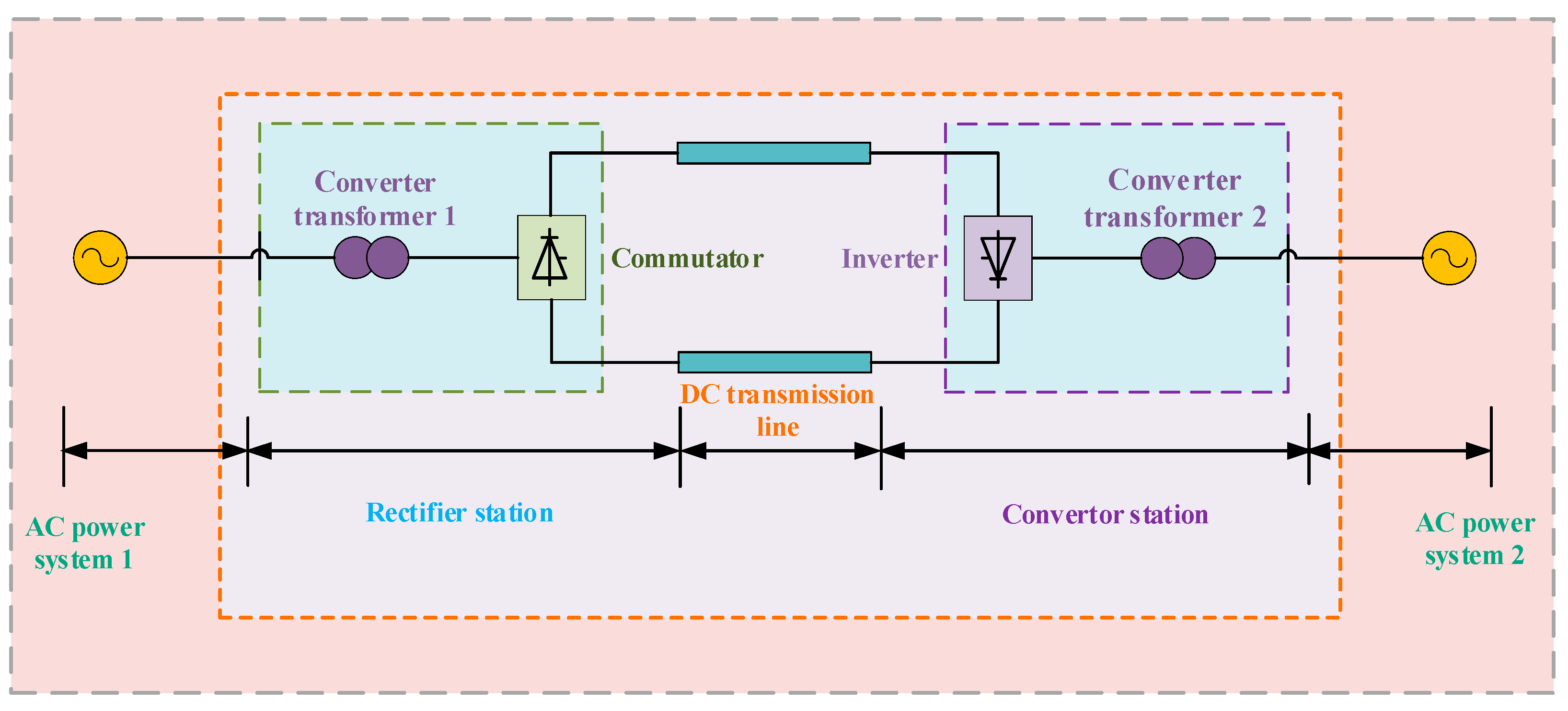
Figure 1. Schematic diagram of HVDC structure.
Energies 18 06253 g001
Figure 2. Geographical location map of the HVDC system.
Energies 18 06253 g002
Figure 3. Distribution of main fault points.
Energies 18 06253 g003
Figure 4. The flowchart of fault diagnosis.
Energies 18 06253 g004
Figure 5. Confusion matrices of comparative experimental results.
Energies 18 06253 g005aEnergies 18 06253 g005b
Figure 6. ROC curves for four types of faults.
Energies 18 06253 g006
Figure 7. Confusion matrices of ablation experiment results of the MSF-LightGBM algorithm.
Energies 18 06253 g007aEnergies 18 06253 g007b
Figure 8. Sensitivity analysis results of the main parameters of MSF-LightGBM.
Energies 18 06253 g008
Figure 9. Feature importance result diagram.
Energies 18 06253 g009
Table 1. Fault types at fault points in a substation.
Fault PointFault TypeFault PointFault Type
F1A/B/C phase groundF11D valve short circuit
F2Interphase short circuitF12Valve short circuit
F3Interphase short circuitF13Y valve high voltage side fault
F4A/B/C phase groundF14High voltage bus fault
F5A/B/C phase groundF15Neutral bus fault
F6Y bridge short circuitF16Line ground
F7Y-D midpoint failureF17Neutral bus disconnection
F8D bridge short circuitF18Neutral bus ground
F9Y valve low
Voltage side fault
F19Ground pole line disconnection
F10Y valve short circuitF20Ground pole line ground
Table 2. Signal channels and their physical meanings [22].
SignalDescription MeaningSignalDescription Meaning
UACA(V)A-phase AC voltageIACD_L3(A)C-phase AC current of D-bridge valve side
UACB(V)B-phase AC voltageUDL(V)DC line voltage
UACC(V)C-phase AC voltageUDN(V)Neutral bus voltage
IACY_L1(A)A-phase AC current of Y-bridge valve sideIDN(A)Neutral bus current
IACY_L2(A)B-phase AC current of Y-bridge valve sideIDE(A)Grounding pole bus current
IACY_L3(A)C-phase AC current of Y-bridge valve sideIDH(A)High-voltage bus current
IACD_L1(A)A-phase AC current of D-bridge valve sideIDL(A)DC line current
IACD_L2(A)B-phase AC current of D-bridge valve side
Table 3. Algorithm parameter table.
TypesParametersValue
LightGBMnum_class4
num_leaves31
learning_rate0.05
feature_fraction0.9
bagging_fraction0.8
bagging_freq5
Multimodalimage_size32
batch_size32
epochs100
learning_rate0.001
LSTMunits128
dropout_rate0.2
learning_rate0.001
epochs100
batch_size8
num_layers2
SVMC2
kernelrbf
gammascale
KNNn_neighbors15
weightsuniform
leaf_sizeleaf_size
p1
n_estimators30
RFmax_depth3
min_samples_split20
min_samples_leaf10
max_features0.3
1D-CNNlearning_rate0.001
dropout_rate0.2
output dimension of fully connected layer4
batch_size8
epochs50
convolution kernel size3
Table 4. Fault diagnosis results of HVDC under different methods.
TypesPrecisionAccuracyRecallF1-ScoreBalanced Accuracy
MSF-LightGBM0.96430.95830.96430.96150.9752
Multimodal0.78750.79170.79290.78100.8620
LSTM0.51360.58330.60830.54710.7346
SVM0.84520.83330.84520.84520.8940
KNN0.67190.54170.52500.50630.6828
RF0.88750.87500.88100.88180.9188
LightGBM0.84520.83330.84520.84520.8940
1D-CNN0.83480.79170.80360.79170.8666
Table 5. Results of evaluation indicators for the ablation experiment.
TypesPrecisionAccuracyRecallF1-ScoreBalanced Accuracy
MSF-LightGBM0.96430.95830.96430.96150.9752
No feature selection0.93750.91670.92860.92260.9504
No feature extraction0.62500.62500.62620.62420.7497
No data augmentation0.08330.33330.25000.12500.500
Table 6. Results of leave-one-(original)-event cross-validation.
RoundTest EventAccuracy
1AC faults_10.4
2AC faults_21.0
3AC faults_31.0
4AC faults_41.0
5AC faults_50
6DC faults_11.0
7DC faults_20.2
8DC faults_31.0
9DC faults_41.0
10DC faults_51.0
11DC faults_60.8
12DC faults_71.0
13converter valve faults_11.0
14converter valve faults_21.0
15converter valve faults_31.0
16converter valve faults_41.0
17converter valve faults_51.0
18converter valve faults_61.0
19converter valve faults_71.0
20inverter commutation failures_10
21inverter commutation failures_20
22inverter commutation failures_31.0
23inverter commutation failures_41.0
24inverter commutation failures_51.0
25inverter commutation failures_61.0
26inverter commutation failures_71.0
27inverter commutation failures_81.0
28inverter commutation failures_90.6
Mean Value/0.821
Disclaimer/Publisher’s Note: The statements, opinions and data contained in all publications are solely those of the individual author(s) and contributor(s) and not of MDPI and/or the editor(s). MDPI and/or the editor(s) disclaim responsibility for any injury to people or property resulting from any ideas, methods, instructions or products referred to in the content.