Integration of Machine Learning-Based Demand Forecasting and Economic Optimization for the Natural Gas Supply Chain

Abstract

This paper proposes a profit optimization method for the natural gas industry chain driven by demand forecasting. The method mainly consists of two core components: the construction of a natural gas demand forecasting model and the solution of an industry chain profit optimization model. In the forecasting stage, three models are trained using historical natural gas demand data, and the optimal model is selected based on performance evaluation indicators to predict natural gas demand for the coming month. In the optimization stage, the physical and operational characteristics of key components in the natural gas pipeline network are fully considered, and a nonlinear programming model is formulated with the objective of maximizing the overall profit of the industry chain. The model is validated using historical data. Finally, the demand forecast results are incorporated into the optimization model to calculate the expected industry chain profit for the next month. The findings of this study can provide theoretical foundations and quantitative decision-making support for natural gas suppliers to develop more economically efficient gas supply strategies.

1. Introduction

1.1. Research Background

With the growing global emphasis on green development strategies, the exploitation and utilization of sustainable energy sources have become a key issue in the energy sector. Natural gas, due to its high efficiency, cleanliness, and stability, has been widely applied in power generation, industrial production, and residential heating. Its role in the global energy system is continuously increasing, making it a crucial driver of low-carbon energy transition.

However, natural gas is not only a clean energy source but also a commodity that requires exploration, production, transportation, storage, and sales, all of which are interdependent and tightly linked to form a highly complex industrial chain. With rising demand and rapidly changing market conditions, the challenge of improving the overall efficiency of the natural gas industry chain through scientific modeling and optimization—while ensuring supply–demand balance—has become increasingly critical. This issue is directly linked to the security and stability of energy systems as well as to the profitability and competitiveness of enterprises. The pipeline network, as the hub of the natural gas industry chain, undertakes the task of receiving upstream supply and delivering it to downstream users, while also facilitating inter-regional gas transfers [1].

The natural gas industry chain, encompassing exploration, production, transportation, and sales, is one of the cornerstones of the global economy and financial markets [2]. As a strategic energy source, natural gas has a profound impact on economic growth and industrial development worldwide. However, under conditions of increasing market uncertainty [3] and intensified competition [4], managing and operating the natural gas industry chain faces new challenges. These challenges not only affect related enterprises but may also threaten the stability of the global natural gas market. Therefore, accurately identifying and responding to these challenges, and formulating effective strategies, are of vital importance for industry operators [5]. Since the “14th Five-Year Plan,” China’s natural gas production has continued to rise, with an annual increase exceeding 100 × 10⁸ m³ [6]; At the same time, the country’s external dependence on natural gas has surpassed 40%, and the sales market has become increasingly complex, demanding a more advanced marketing and operational system [7]. With natural gas demand steadily increasing, the question of how to balance stable supply with profitability has become a core issue for decision-making in natural gas enterprises.

1.2. Literature Review

1.2.1. Demand Forecasting

Natural gas demand is influenced by a variety of factors, including temperature, economic development, population growth, and even political conditions, which makes it highly seasonal and volatile. Accurate forecasting of natural gas demand is therefore crucial. Without reliable forecasts, it is difficult to formulate reasonable supply and dispatching strategies, which would negatively affect supply–demand matching and the overall efficiency of the industry chain. Demand forecasting not only provides key input data for calculating downstream user requirements but also establishes the foundation for setting constraints and objective functions in optimization models. Thus, demand forecasting plays a fundamental role in natural gas industry chain modeling, directly influencing the scientific nature of supply planning, the rationality of resource allocation, and the reliability of end-user supply [8]. Accurate and robust forecasting can effectively prevent resource waste and avoid supply–demand imbalances [9]. As natural gas is increasingly becoming a dominant clean energy source, its demand trends have become essential references for energy system planning, emergency protection, and policy-making. Forecast results not only affect enterprise operational profits but also exert a profound influence on energy dispatching and strategic reserves [10,11].

The time-series characteristics and seasonality of natural gas demand, coupled with its volatility and multi-factor interactions, pose great challenges to forecasting. In recent years, with the rise in machine learning, data-driven approaches have been widely applied in demand forecasting [12,13,14]. Models such as XGBoost, Random Forest (RF), and Support Vector Regression (SVR) have demonstrated strong robustness in handling nonlinear, multivariate problems and complex data structures [15,16,17,18]. Compared with traditional statistical methods, data-driven models can more effectively capture nonlinear patterns and adapt to complex market conditions, thus providing higher prediction accuracy. Anagnostis A et al. [19] demonstrated that Long Short-Term Memory (LSTM) networks can effectively forecast daily natural gas demand; Sharma V et al. [20] adopted a block-based modeling strategy, training different models for different time intervals within a day, and combining them to significantly improve forecast performance. For complex systems such as industry or supply chains, machine learning models applied to the demand side can help optimize resource allocation and guide enterprises in adjusting supply strategies accordingly [21,22].

1.2.2. Optimization Model Research

Optimization techniques have played a vital role in balancing gas supply and profitability. Current methodologies for constructing natural gas industry chain optimization models can generally be categorized into two approaches: The first approach is algorithm-driven, which formulates objective functions and system constraints to directly determine the optimal configuration of key operational parameters in pipeline networks; The second approach is simulation-driven, depending on the type of system being modeled—whether a single pipeline or a complex network—these simulation tools can be further categorized [23]. Some software can utilize input parameters such as operating pressure and temperature as boundary conditions to solve for the pressure distribution at each node and determine real-time operational parameters of key equipment, such as compressors and pressure regulation stations. This provides quantitative support for operational decision-making. With the advancement of China’s “National Gas Pipeline Network” integration strategy, the structure of natural gas pipeline systems has become more complex, featuring higher interconnectivity and enhanced flexibility in cross-regional gas allocation. While creating new optimization opportunities, this evolution increases modeling complexity for supply–demand coordination: more system variables and coupled relationships elevate data dimensionality and computational demands. Consequently, manual or pipeline-by-pipeline balancing methods have become inadequate. Al-Zalitani et al. [24] noted their limited applicability to intricate, branched pipeline systems. Meanwhile, existing studies on China’s “National One Network” construction have demonstrated that the integrated pipeline system further increases model coupling complexity and highlights the necessity of developing unified optimization frameworks capable of handling cross-regional transmission coordination [25]. Therefore, there is an urgent need for new analytical and modeling approaches capable of addressing the “national unified network” framework.

Early studies focused on optimizing gas supply and transportation, developing diverse modeling approaches under different objective functions. Common objectives included maximizing sales company profits via linear programming or optimizing integrated production-transportation-sales synergies through system-wide mathematical abstraction [26,27].

As market competition intensified, both objective functions and modeling methods have diversified. Single economic metrics evolved into multi-objective frameworks incorporating profit, customer satisfaction, and supply reliability. Additional objectives included cost minimization, energy efficiency maximization, and carbon emission constraints. Beyond classical linear/nonlinear programming, mixed-integer programming addressed discrete decisions, while stochastic programming and robust optimization handled demand/price uncertainties. Moreover, game theory has been applied to capture competitive and cooperative dynamics among multiple stakeholders, enabling the industry chain to reach equilibrium solutions. Such approaches enrich the theoretical foundations of optimization while balancing profitability with service quality [28,29].

At the international level, research has placed greater emphasis on cross-regional system optimization and overall value chain enhancement. Scholars are increasingly focusing on the optimization of cross-regional supply systems and the enhancement of the natural gas industry chain’s value. They are committed to improving the resilience, efficiency, and value-added performance of the entire natural gas industry through the optimization of resource allocation and operational strategies. Studies have investigated collaborative scheduling of infrastructure using multi-period MIP models to minimize total system costs or maximize overall benefits, as well as optimization of upstream logistics (transportation and storage) to enhance resource flexibility and ensure supply security. Meanwhile, hybrid approaches that combine heuristic algorithms with exact optimization methods have also been explored, demonstrating the advantages of multi-method integration for profitability in complex natural gas systems [30,31,32,33].

In summary, both domestic and international research has contributed substantially to demand forecasting and industry chain optimization, providing a solid theoretical and methodological foundation for more scientific and intelligent operations. However, limitations remain: most studies have focused on upstream supply and transportation, with insufficient attention to the differentiated needs of downstream users. This gap reduces the adaptability of optimization results at the consumer level, which is critical for effective supply–demand matching and profit maximization [34,35]. Furthermore, many studies rely heavily on retrospective modeling [11], lacking predictive, forward-looking mechanisms to handle future demand fluctuations and market dynamics [36]. Finally, as the global energy transition continues to accelerate, worldwide natural gas demand is experiencing sustained annual growth. In 2024 alone, the year-on-year increase in global natural gas demand reached 2.7%, significantly exceeding the average annual growth rate observed between 2010 and 2019 [37]. In light of amplified volatility in natural gas markets, climate change, and policy adjustments—all contributing to external uncertainties—most existing models lack systematic risk characterization and robust optimization design, thus limiting their applicability in complex and uncertain environments [38,39,40].

1.3. Research Objectives

To address the identified research gaps, this study aims to develop a novel, integrated methodological framework that seamlessly combines demand forecasting with operational optimization to maximize the profit of the natural gas industrial chain. The specific research objectives are defined as follows:

(1) To develop an accurate short-term demand forecasting model for downstream natural gas users. This involves preprocessing historical consumption data to handle noise and missing values, and then training and evaluating multiple machine learning models (XGBoost, Random Forest, and SVR) to identify the most reliable predictor for daily demand in the upcoming month.

(2) To construct a comprehensive profit-maximization model for the natural gas industrial chain. This model will incorporate the physical and operational constraints of all key components within the pipeline network (e.g., gas sources, pipelines, storage facilities, LNG terminals, and end-users). The objective function will be formulated to maximize the total economic profit, encompassing sales revenue, resource supply costs, and transportation expenses.

(3) To validate the proposed integrated framework through a real-world case study. This objective involves utilizing historical data to verify the feasibility of the optimization model and, most importantly, integrating the forecasted demand results into the optimization model to calculate and analyze the expected profit for the subsequent month. The ultimate goal is to provide a quantitative decision-support tool for natural gas suppliers.

1.4. Contribution and Organization

To address the above-mentioned research gaps, this paper proposes a profit optimization method for the natural gas industry chain that is driven by demand forecasting. By embedding user demand forecasts into the optimization model, this method enables dynamic assessment and forward-looking optimization of industry chain profitability, thereby providing new approaches and methodologies for scientific decision-making under complex environments. The proposed framework mainly consists of two components: construction of natural gas demand forecasting models and solution of the industry chain economic profit optimization model. The main contributions of this study are summarized as follows:

(1) Based on historical demand data of downstream users, three commonly used models—XGBoost, Random Forest (RF), and Support Vector Regression (SVR)—were trained. A comprehensive comparison of model performance was conducted, and the best-performing model was selected. Using this model, natural gas demand for the upcoming month was forecasted, yielding specific numerical values of predicted demand.

(2) A natural gas industry chain optimization model was established. In terms of constraints, six types of key components in the pipeline network (gas sources, users, storages, LNG terminals, pipelines, and stations) were explicitly modeled according to their distinct functions. The objective function was defined as the maximization of the overall economic benefit of the industry chain, resulting in a complete optimization framework.

(3) A case study was conducted to verify the feasibility of the optimization model using historical downstream user demand data. Subsequently, the demand forecast results from the first part were integrated into the optimization model as key inputs. The model was then solved to produce the expected profit outcomes of the natural gas industry chain for the following month. These results provide quantitative decision-making support for short-term gas supply planning and market strategies.

The remainder of this paper is organized as follows: Section 2 presents the theoretical background of the proposed methodology, including data preprocessing, demand forecasting models, performance evaluation metrics, and the construction of the optimization model. Section 3 provides detailed results of data processing, evaluates the training effectiveness of the three candidate models, selects the optimal forecasting model, and validates the optimization framework using case studies. This section also integrates demand forecast results into the optimization model to calculate expected industry chain profits. Section 4 summarizes the findings, highlights key conclusions, and discusses current limitations of the research as well as potential directions for future improvement.

2. Methodology

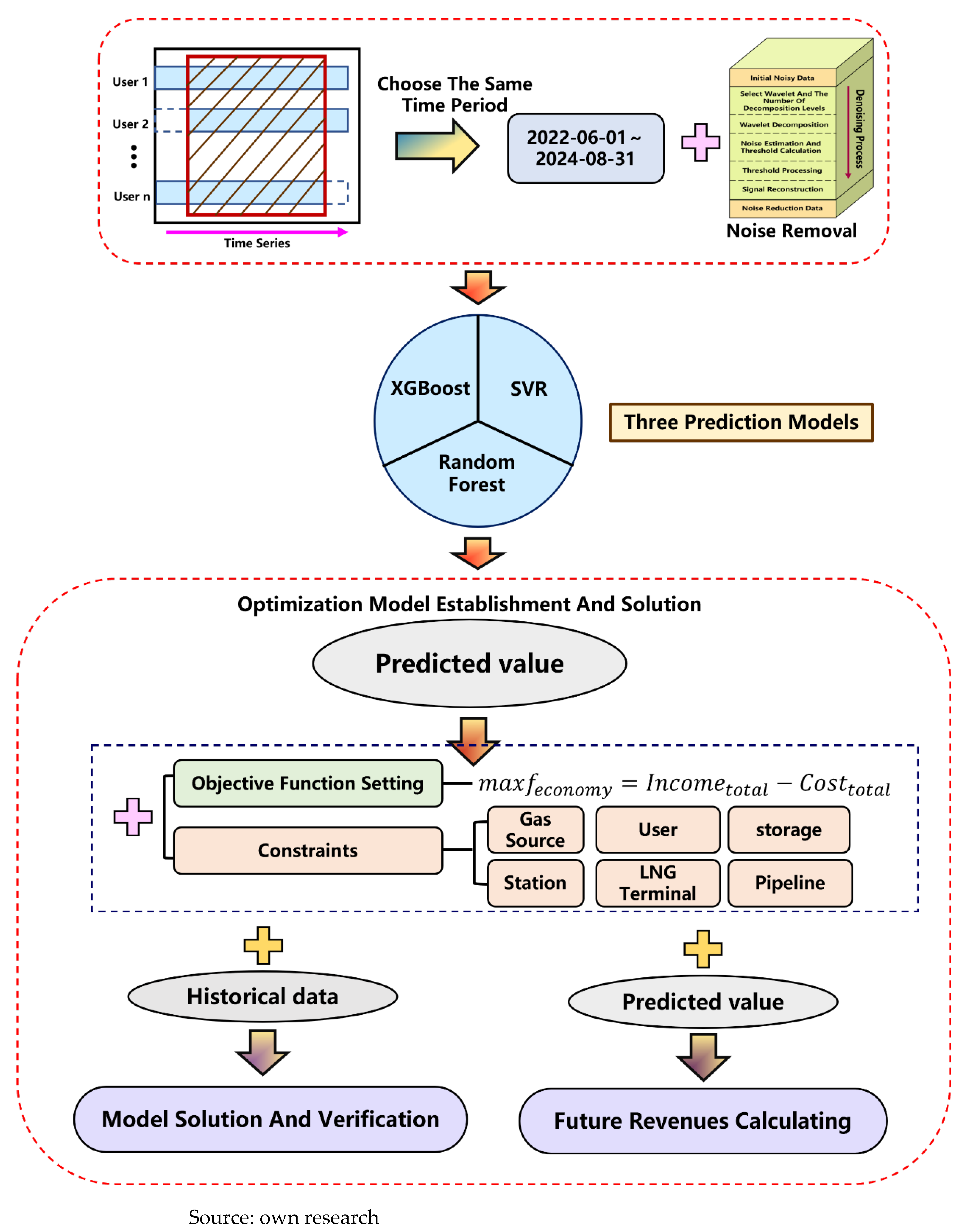
The research methodology of this paper is illustrated in Figure 1. Section 2.1 and Section 2.2 focus on the time-series characteristics of user demand for natural gas, filtering effective historical data with complete temporal coverage and applying denoising techniques to construct a high-quality dataset. Based on this dataset, three machine learning algorithms—XGBoost, RF, and SVR—are used to build natural gas demand forecasting models. The models are evaluated using three metrics, MAE, MAPE and R², and the best-performing model is selected. This model is then used to predict daily natural gas demand for the next 30 days.

In Section 2.3, The model incorporates the functional and operational characteristics of key components in the natural gas pipeline network and defines the objective function as maximizing the overall economic profit of the industry chain. By coupling demand forecasting with economic optimization objectives, the proposed framework achieves global profit maximization under differentiated demand patterns across different user groups and time windows (e.g., intraday and interday), thereby enhancing both the economic rationality and operational feasibility of gas supply strategies.

2.1. Data Intersection Calculation and Noise Removal

Accurate identification of user demand patterns is essential for constructing profit optimization models and determining optimal supply strategies. An in-depth analysis of end-user historical natural gas consumption behavior is a critical step in constructing economic optimization models, as well as a core component for identifying optimal supply strategies under economically maximized conditions. Within this context, accurately forecasting potential user demand serves as a fundamental prerequisite, necessitating the development of demand prediction models supported by historical data. However, the practical data collection process is often challenged by issues such as poor data quality and missing values, with incomplete time series (missing data points or temporal gaps) and high-noise interference (outliers, measurement errors) being particularly prominent. This situation underscores the necessity of preprocessing raw data through techniques such as imputation and denoising.

To ensure the reliability of subsequent predictive modeling, the raw data were processed as follows First, historical natural gas consumption data from users with consistent observation periods were selected based on the principle of temporal consistency, thereby eliminating heterogeneity in data spans. Subsequently, wavelet denoising technique was applied to the homogeneous-period dataset to filter out noise, significantly enhancing data quality. The methods employed are detailed in Section 2.1.1 and Section 2.1.2.

2.1.1. Data Intersection Calculation

During the data preprocessing stage prior to model training, standardizing the time intervals of temporal data is crucial for ensuring model accuracy. For the collected user demand time series dataset—covering the period from 1 April 2020 to 31 August 2024—non-uniform observation periods can significantly impair the model’s generalization capability. To address this, the observation windows of all user data were synchronized using Equation (1), ultimately yielding a maximum common valid time period shared across all users (1 June 2022 to 31 August 2024). This process ensures that the input data for the predictive model possess consistent temporal characteristics, thereby fundamentally eliminating modeling biases caused by inconsistent start and end times of the sequences.

$$D_{common}=\underset{u}{\cap }D(u)$$

(1)

In the equation, $D_{common}$ denotes the date values common to all users, $D(u)$ represents the date values across all users. The processed data structure conforms to the input requirements of the subsequent predictive model.

After aligning time windows (June 2022–August 2024), linear interpolation and seven-day moving average smoothing were applied to maintain temporal continuity and remove artificial discontinuities caused by intersection truncation. Lag-lead correlation tests between end-user demand and storage operations confirmed that dynamic dependencies were preserved, ensuring that storage units retain realistic “memory” behavior over consecutive days.

2.1.2. Wavelet Threshold Denoising

Although the data meet structural requirements, the historical natural gas demand dataset still contains certain values that deviate from the overall trend, i.e., noisy data. Therefore, it is essential to perform necessary denoising procedures to enhance data quality and reliability.

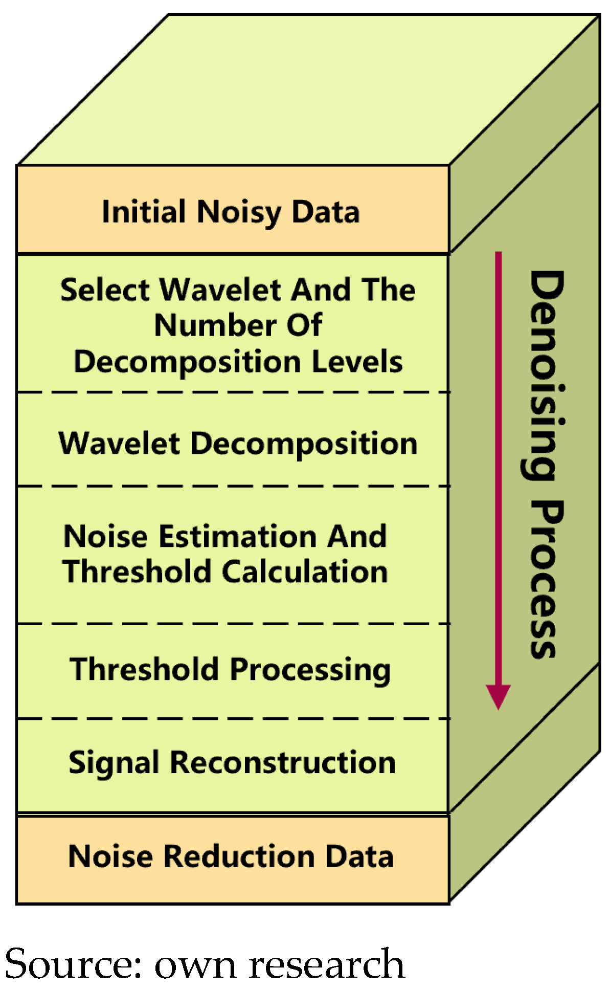
To address the collected multi-user time series data, and considering the characteristics of natural gas demand data influenced by short-term random factors and business cycles, wavelet denoising technique was selected for processing the original data. Its core advantage lies in the accurate separation of trends, cycles, and noise. Moreover, its adaptive threshold rule effectively suppresses noise while preserving critical information in the data. The localized nature of wavelet denoising enables precise identification and processing of dynamic variations at different times and frequencies within non-stationary signals, making it particularly suitable for handling time-varying non-stationary factors such as weather, market conditions, and holidays that affect natural gas supply. This approach helps accurately capture the underlying patterns from mixed data, providing clean and reliable input for high-precision demand forecasting models. The basic workflow of wavelet denoising is clearly illustrated in Figure 2.

2.2. Training and Evaluation of Prediction Models

To achieve economically optimal decision-making in the natural gas supply chain, it is essential to accurately forecast future demand trends. The historical data, after undergoing the fundamental processing described above, now meet the input requirements for predictive models. In Section 2.2.1, systematic modeling and analysis are conducted for three typical time series forecasting models; Section 2.2.2 discusses how to quantitatively evaluate the training performance of each model and ultimately identify the optimal forecasting model.

2.2.1. Introduction to the Prediction Model

(a)

XGBoost

In downstream user demand forecasting, historical data often contain missing values and noise, while variables such as temperature, date, and holidays frequently exhibit complex nonlinear relationships. Traditional linear methods demonstrate clear limitations in capturing such intricate nonlinear patterns, thus often failing to meet the accuracy requirements for natural gas demand prediction. In contrast, the XGBoost model enhances prediction robustness and accuracy by iteratively optimizing residuals and possessing a built-in capability to handle missing values.

For the preprocessed data, a 7-day sliding window was employed for feature construction, using the demand values from the past seven days as input to predict the demand on the eighth day. The last month of the historical dataset was allocated as the test set, with the remainder serving as the training set. This partitioning simulates the real-world scenario of “using historical data to forecast future values.” During the training phase, the model iteratively optimizes the objective function by adjusting leaf weights to fit the characteristics of the historical data. The objective function incorporates both a loss function and a structural regularization term, as specified in Equations (2) and (3).

$$\mathrm{\Gamma }(\theta )={\displaystyle {\sum }_{i}L}(y_i,{\widehat{y}}_i)+{\displaystyle \sum _k\mathrm{\Omega }(f_k)}$$

(2)

$$\mathrm{\Omega }(f_k)=\gamma T+{\displaystyle \frac{1}{2}}\lambda {‖\omega ‖}^2$$

(3)

In the equation, $\mathrm{\Gamma }(\theta )$ represents objective function; $L(y_i,{\widehat{y}}_i)$ represents the loss value during training, $y_i$ is the true value of the i-th sample, ${\widehat{y}}_i$ denotes the quantified predicted value of the i-th sample; $\mathrm{\Omega }(f_k)$ is the regularization term; T is the number of leaf nodes, $\omega$ is the leaf weight vector, $\gamma$ is the complexity threshold for splitting, $\lambda$ is the penalty coefficient applied to the weights.

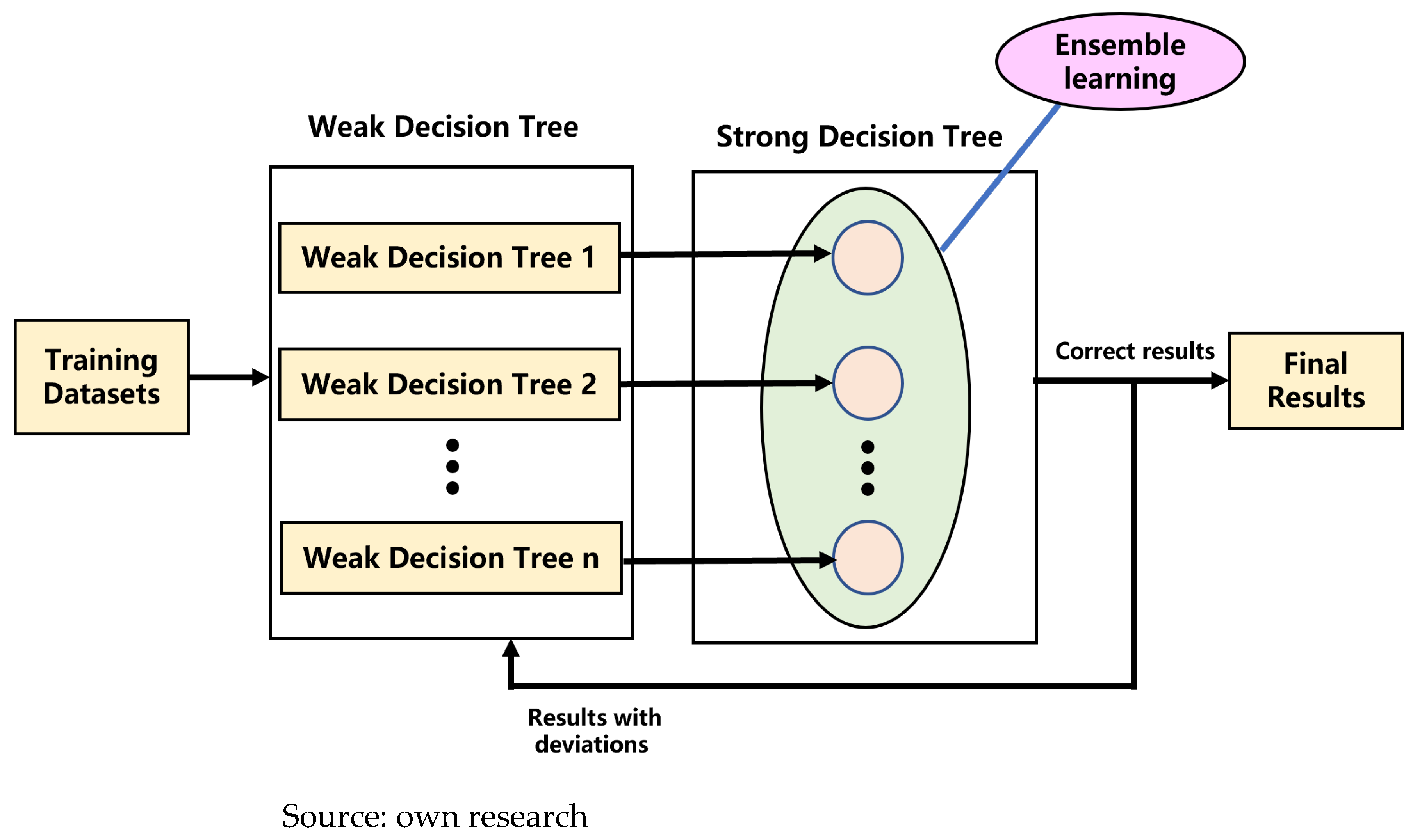
In terms of parameter configuration, during the validation phase, the number of base learners was set to 50 while keeping the remaining parameters at their default values to prevent overfitting under limited sample conditions and ensure convergence stability. For the 30-day rolling prediction, the parameters were adjusted to enhance the model’s expressive capacity: the number of base learners was increased to 500, the maximum tree depth was set to 6, and the learning rate was set to 0.05. This “lightweight training, full-capacity prediction” strategy enables the model to stably fit historical data while maintaining high accuracy in long-term forecasting. The overall workflow of the XGBoost model training process is illustrated in Figure 3.

(b)

Random Forest (RF)

Random Forest is a typical ensemble learning method that generates multiple decision trees through random sampling of both instances and features, and produces outputs in an integrated manner. Its structure ensures predictive accuracy while enhancing the model’s generalization capability, making it suitable for modeling multi-source variables and nonlinear relationships in natural gas demand forecasting. The formula for calculating predicted values obtained through the Random Forest model is given in Equation (4).

$$\widehat{y}={\displaystyle \frac{1}{K}}{\displaystyle \sum _{k=1}^K{T}_k(x;{\mathrm{\Theta }}_k)}$$

(4)

In the equation, $\widehat{y}$ represents the final predicted value generated by the model; K denotes the number of decision trees; $T_k$ refers to the prediction function of the kth tree, ${\mathrm{\Theta }}_k$ indicates the parameters of the kth tree. Additionally, the Random Forest model is capable of computing the importance ranking of each feature in the prediction process, thereby identifying key driving factors behind demand variations. This feature aids in uncovering disparities among different user groups in the downstream market.

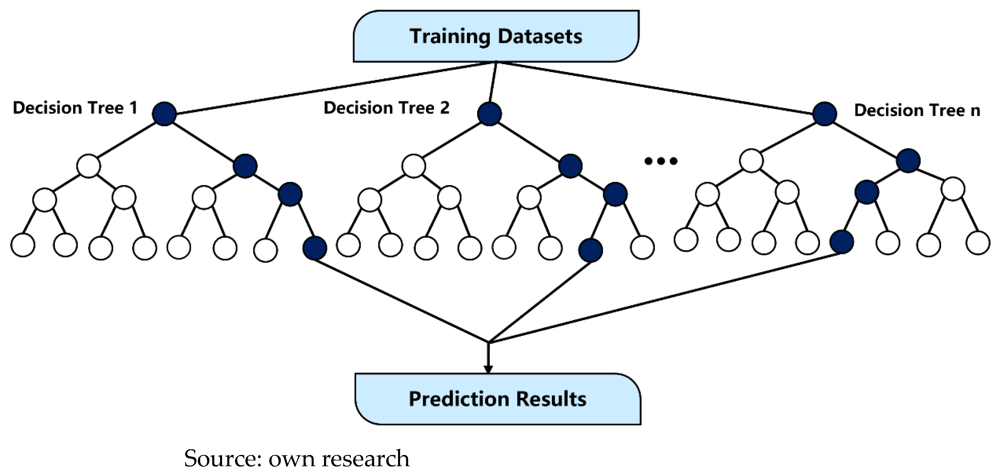
During the training process, the preprocessed historical natural gas demand data were also used to construct features via the same sliding window approach of “using the first seven days to predict the eighth,” as described in the XGBoost section. The training and test sets were partitioned identically to that in the XGBoost model. For the validation phase, the parameters were configured as follows: number of trees set to 300, maximum tree depth to 15, and random seed to 42. This configuration ensures both diversity within the forest and prediction stability. For the 30-day rolling prediction, the parameters were adjusted to 500 trees and a maximum depth of 12 to enhance robustness in long-term forecasting. The workflow of the Random Forest model training process is illustrated in Figure 4.

The Random Forest method offers notable advantages, including robustness to outliers and missing values, as well as the capability to handle high-dimensional and multi-source input data. Furthermore, by leveraging its feature importance output, it becomes possible to quantify the contribution of factors such as temperature and date to demand fluctuations, thereby providing valuable decision-making support for enterprises.

(c)

Support Vector Regression (SVR)

Natural gas demand often exhibits short-term sharp fluctuations under extreme weather or emergency conditions, which imposes higher requirements on the stability of forecasting models. Traditional statistical models, however, are susceptible to disturbances from outliers in such scenarios, leading to reduced prediction accuracy. Support Vector Regression (SVR) addresses this by employing kernel functions to map data into a high-dimensional space and fitting the majority of sample points within an error tolerance band, thereby ensuring smooth and robust prediction outcomes. Its “insensitive band” mechanism is particularly effective in suppressing the impact of short-term outliers on overall forecasting. The objective function of the SVR model aims to minimize the norm of the weight vector and the penalty term on slack variables, as shown in Equation (5).

$$\min {\displaystyle \frac{1}{2}}{‖\omega ‖}^2+C{\displaystyle \sum _{i=1}^n({\xi }_i+{\xi }_i^{\ast })}$$

(5)

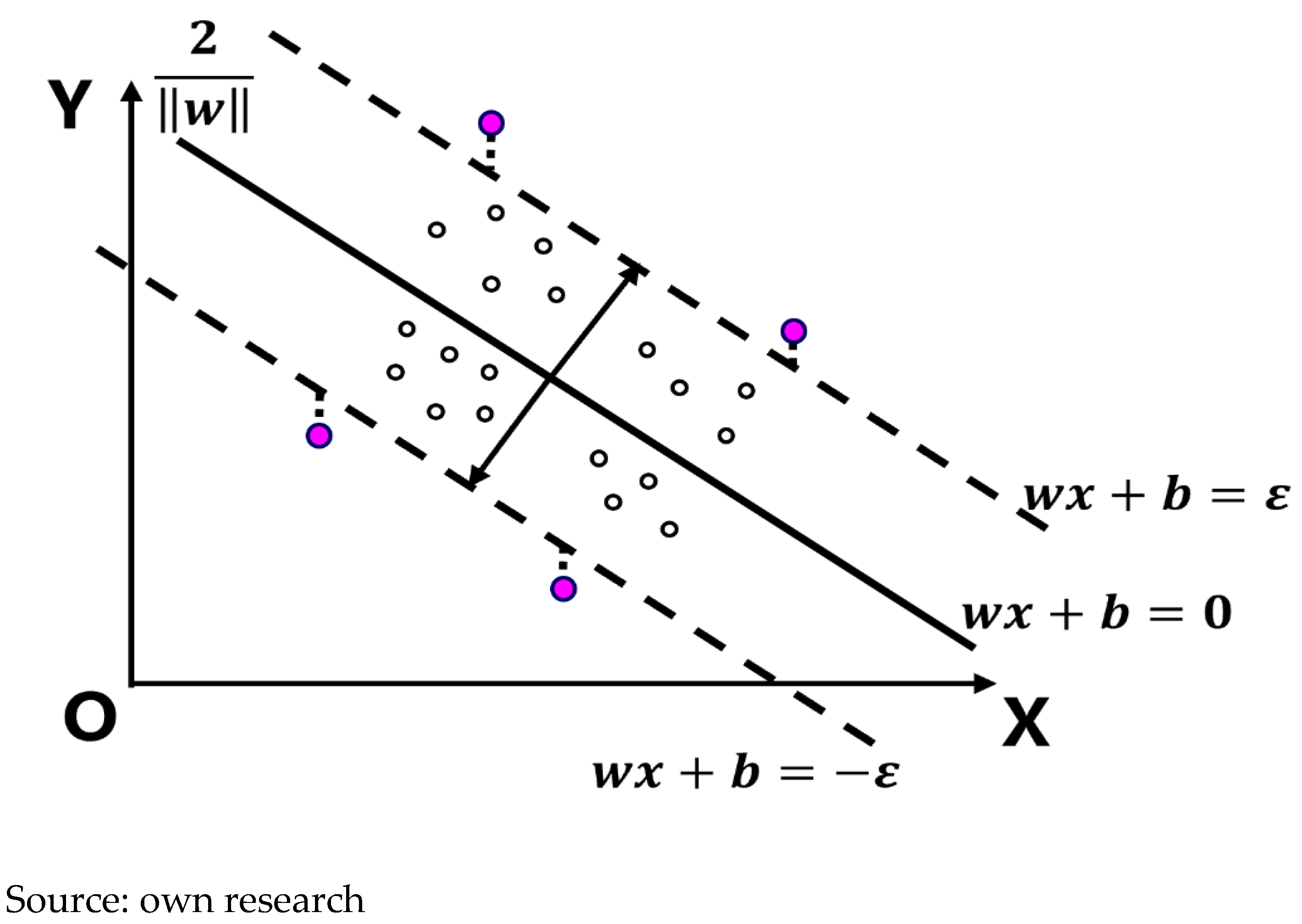
In the equation, ${\displaystyle \frac{1}{2}}{‖\omega ‖}^2$ denotes the regularization term; C is the penalty coefficient, which balances the trade-off between model complexity and training error; ${\xi }_i$ refers to the upper-bound slack variable for the ith sample, ${\xi }_i^{\ast }$ represents the lower-bound slack variable for the ith sample. Figure 5 illustrates the solution range of the SVR model. The values within the dashed lines constitute the correct solution range of SVR, also known as the ε (error tolerance). The values outside the dashed lines represent larger errors and are referred to as support vectors, which determine the complexity and generalization capability of the SVR model.

Following the same procedure as applied to the XGBoost and Random Forest models, the preprocessed data were divided into training and test sets, and a seven-day sliding window was used to construct supervised learning samples. First, a grid search was performed on the training set with an initial parameter range: the penalty coefficient C was set to {0.1, 1, 10, 100, 1000}, the insensitive band ε was set to {0.01, 0.05, 0.1, 0.2}, and the kernel width γ to {‘scale’, ‘auto’, 0.01, 0.1, 1}. The optimal model configuration within this parameter space was identified. Subsequently, the full historical dataset was retrained using the optimal parameters to ensure the model could capture temporal patterns of demand with a larger volume of data. Based on this retrained model, a day-by-day iterative approach was employed to conduct a 30-day rolling forecast of future demand. This process used the most recent seven days of both actual and predicted values as input to generate predictions for the next time step sequentially. To improve computational efficiency and avoid over-searching during the prediction phase, the parameter optimization range was narrowed compared to the initial training stage. The refined parameter set was limited to: penalty coefficient C set to {0.1, 1, 10, 100}, insensitive band ε to {0.01, 0.05}, and kernel width γ to {‘scale’, ‘auto’, 0.01, 0.1, 1}.

This two-phase strategy of “wide-range exploration followed by narrowed refinement” not only ensures the stability and accuracy of model predictions but also reduces computational overhead during rolling forecasting, effectively balancing parameter optimization and prediction efficiency.

2.2.2. Model Evaluation Criteria

For the three aforementioned models, the processed historical natural gas demand data from downstream users were used as input. The last month of the historical dataset was allocated as the test set, with the remainder serving as the training set.

The ex-post errors reported in this study were calculated for a one-day-ahead forecast. Specifically, during both the training and testing phases, each model’s input was a 7-day historical sliding window (days t−7 to t−1), and the output was the predicted demand for the next single day (day t). This one-step-ahead forecasting approach is aligned with the short-term operational decision-making needs of the natural gas industry.

The models were evaluated based on six metrics: Mean Error (ME), Mean Absolute Error (MAE), Mean Absolute Percentage Error (MAPE), Mean Percentage Error (MPE), Root Mean Square Error (RMSE) and the Coefficient of Determination (R²). The mathematical expressions for these metrics are provided in Equations (6), (7), (8), (9), (10) and (11), respectively.

$$ME={\displaystyle \frac{1}{n}}\ast {\displaystyle \sum (y_i-{\widehat{y}}_i)}$$

(6)

$$MAE={\displaystyle \frac{1}{n}}\ast {\displaystyle \sum \left|y_i-{\widehat{y}}_i\right|}$$

(7)

$$MAPE={\displaystyle \frac{100\%}{n}}\ast {\displaystyle \sum \left|\frac{y_i-{\widehat{y}}_i}{y_i}\right|}$$

(8)

$$MPE={\displaystyle \frac{100\%}{n}}\ast {\displaystyle \sum \left|\frac{y_i-{\widehat{y}}_i}{{\widehat{y}}_i}\right|}$$

(9)

$$RMSE=\sqrt{({\displaystyle \frac{1}{n}})\ast {\displaystyle \sum {(y_i-{\widehat{y}}_i)}^2}}$$

(10)

$$R^2=1-({\displaystyle \frac{{\displaystyle \sum {(y_i-{\widehat{y}}_i)}^2}}{{\displaystyle \sum {(y_i-\overline{y})}^2}}})$$

(11)

In the equations, n denotes the sample size; $y_i$ represents the true value of the ith sample; ${\widehat{y}}_i$ indicates the predicted value of the ith sample; $\overline{y}$ refers to the mean value of the target variable.

When ME and MPE get closer to 0, MAE, MAPE and RMSE exhibit low values while R² approaches 1, it indicates strong performance of the model in terms of predictive bias control and goodness-of-fit, making it a suitable candidate solution for the final forecasting model.

2.3. Optimize Model Constructing

The operation of the natural gas industry chain is inherently a dynamic process involving the coupling of multiple factors, where operational economic efficiency is influenced by a variety of elements. With the core objective of maximizing operational economic benefits, enterprises in the industry chain must develop corresponding gas supply plans based on the differentiated natural gas demand of downstream users. Given that some companies have already established relatively mature gas supply planning systems, it is essential to conduct proactive forecasting of downstream market natural gas demand. This enables sufficient flexibility in practical operations, allowing supply strategies to both meet the diverse needs of downstream users and optimize economic performance.

In this section, a natural gas supply optimization model for the industrial chain is established based on the Gurobi solver by defining boundary conditions and an objective function. Combined with the demand forecasting results obtained in the previous section, the model enables quantitative evaluation of the economic benefits under specific future supply strategies. First, based on the fundamental structure of the natural gas industry chain and incorporating graph theory, the system is abstracted into a network composed of nodes and edges. This network includes six core components: gas sources, end-users, LNG terminals, storage facilities, pipelines, and processing stations. For each component, relevant operational parameters and constraints are defined in accordance with actual industry operational specifications. The detailed configurations are summarized in

Table 1. Parameters of system components.

Component	Functional Parameter	Unit
Gas source	Supply upper limit	104 m3/d
	Planned supply	104 m3/d
	Price	RMB/m3
User	Supply upper limit	104 m3/d
	Supply lower limit	104 m3/d
	Planned supply	104 m3/d
	Price	RMB/m3
Storage	Gas withdrawal capacity limit	104 m3/d
	Gas injection capacity limit	104 m3/d
	Gas withdrawal price	RMB/m3
	Gas injection price	RMB/m3
LNG terminal	LNG uploading capacity limit	104 m3/d
	LNG export capacity limit	104 m3/d
	Uploading price	RMB/m3
	Export price	RMB/m3
Pipeline	Pipeline mileage	km
	Transportation capacity limit	104 m3/d
	Transportation price	RMB/m3/km
Station	-	-

Source: own research.

.

It should be noted that the actual significance of the injection and withdrawal flows processes in gas storage facilities and LNG receiving stations is quite different. The injection and withdrawal flows of the gas storage facility refer to the processes of gas injection and extraction; while the injection and withdrawal flows of the LNG receiving station represent a process of receiving LNG resources transported by LNG carriers and then transporting the resources out to the gas transmission network.

The objective function is defined as the maximization of economic efficiency in the operation of the natural gas industry chain. The specific mathematical formulations are provided in Equations (12)–(14).

$$\max f_{economy}=Incom{e}_{total}-Cos{t}_{total}$$

(12)

$$Incom{e}_{total}={\displaystyle \sum (q_{demand}^{i,actual}}\ast pric{e}^i)$$

(13)

$$\begin{array}{l}Cos{t}_{total}={\displaystyle \sum (q_{supply}^{i,actual}\ast pric{e}^s)}+{\displaystyle \sum (q_{pipeline}^{i,actual}\ast L^p\ast pric{e}^p)}\\ +{\displaystyle \sum (q_{storage-in}^{i,actual}\ast pric{e}^{s_{in}})}+{\displaystyle \sum (q_{storage-out}^{i,actual}\ast pric{e}^{s_{out}})}\\ +{\displaystyle \sum (q_{tank-in}^{i,actual}\ast pric{e}^{t_{in}})}+{\displaystyle \sum (q_{tank-out}^{i,actual}\ast pric{e}^{t_{out}})}\end{array}$$

(14)

In the equations above, $f_{economy}$ represents the operational economic revenue of the natural gas industry chain; $Incom{e}_{total}$ denotes the total revenue from natural gas sales to end-users in the downstream market; $Cos{t}_{total}$ refers to the total cost required to maintain the operation of the entire natural gas industry chain; $q_{supply}^{i,actual}$ indicates the actual gas supply volume from the ith gas source; $pric{e}^s$ is the unit price of gas supply from the ith source; $q_{pipeline}^{i,actual}$ represents the actual transportation volume through the ith pipeline; $L^p$ and $pric{e}^p$ denote the length and unit transportation price of the ith pipeline, respectively; $q_{storage-in}^{i,actual}$ and $pric{e}^{s_{in}}$ refer to the actual injection volume and unit injection price of the ith gas storage facility, respectively; $q_{storage-out}^{i,actual}$ and $pric{e}^{s_{out}}$ indicate the actual withdrawal volume and unit withdrawal price of the ith gas storage facility, respectively; $q_{tank-in}^{i,actual}$ and $pric{e}^{t_{in}}$ represent the actual received volume and unit receiving price at the ith LNG terminal; $q_{tank-out}^{i,actual}$ and $pric{e}^{t_{out}}$ denote the actual supply volume and unit supply price from the ith LNG terminal, respectively.

For each component within the network structure, mass balance constraints and operational constraints are applied. The mass balance constraints ensure that the total gas supply from upstream sources equals the total gas delivered to downstream users across the natural gas industry chain. The operational constraints ensure that each component complies with operational specifications, thereby safeguarding the safe and stable operation of the entire system. The following section elaborates on the constraint settings for each component.

(1)

Gas Source:

$$q_{supply}^{i,actual}={\displaystyle \sum q_{pipeline(s\to p)}^{i,actual}}$$

(15)

$$q_{supply}^{i,\min }\le q_{supply}^{i,actual}\le q_{supply}^{i,\max }$$

(16)

Equation (15) specifies that the actual gas supply volume from the ith gas source equals the sum of the actual transportation volumes of all pipelines originating from that source. Equation (16) ensures that the actual gas supply from each source remains within the upper and lower bounds permitted by its supply capacity.

(2)

User:

$$q_{demnad}^{i,actual}={\displaystyle \sum q_{pipeline(p\to d)}^{i,actual}}$$

(17)

$$q_{demand}^{i,\min }\le q_{demand}^{i,actual}\le q_{demand}^{i,\max }$$

(18)

$$q_{demand}^{i,\min }=0.6\ast q_{demand}^{i,\max }$$

(19)

Equation (17) specifies that the actual gas volume received by the ith user equals the sum of the actual transportation volumes of all pipelines terminating at that user. Equation (18) ensures that the actual gas supply to each user remains within the upper and lower bounds defined by the user’s gas reception capacity. Equation (19) further enhances supply continuity and security by setting the lower bound at 60% of the upper bound, thereby guaranteeing a stable baseline gas supply that meets fundamental demand under all operating conditions.

(3)

Storage:

$$0\le q_{storage-in}^{i,actual}\le q_{storage-in}^{i,\max }$$

(20)

$$0\le q_{storage-out}^{i,actual}\le q_{storage-out}^{i,\max }$$

(21)

$$I_{s,t}=I_{s,t-1}+Q_{s,t}^{inj}-Q_{s,t}^{wd}$$

(22)

Equations (20) and (21) specify that the actual injection and withdrawal volumes of the gas storage facility must be non-negative while remaining constrained by the upper bounds of their respective operational capacity limits. In Equation (22), $I_{s,t}$ represents the gas storage volume in the gas storage reservoir at time t, $I_{s,t-1}$ represents the gas storage volume in the reservoir at a certain previous time before time t, $Q_{s,t}^{inj}$ represents the gas injection volume into the reservoir at time t, and $Q_{s,t}^{wd}$ represents the gas extraction volume from the reservoir at time t.

Similar continuity constraints were also imposed on LNG terminals to ensure complete mass balance validation across the system. These additional constraints guarantee that storage operations respect capacity limits and preserve cumulative consistency over time.

(4)

LNG Terminal:

$$0\le q_{tank-in}^{i,actual}\le q_{tank-in}^{i,\max }$$

(23)

$$0\le q_{tank-out}^{i,actual}\le q_{tank-out}^{i,\max }$$

(24)

Equations (23) and (24) specify that the actual received volume and supply volume of the LNG terminal must be non-negative and constrained by the upper limits of its receiving and delivery capacities, respectively.

(5)

Pipeline:

$$0\le q_{pipeline}^{i,actual}\le q_{pipeline}^{i,\max }$$

(25)

Equation (25) specifies that the actual transportation volume of the pipeline must be non-negative and constrained by the upper limit of its transportation capacity.

(6)

Station:

$${\displaystyle \sum q_{station(upstream\to s)}^{i,actual}}={\displaystyle \sum q_{station(s\to downstream)}^{i,actual}}$$

(26)

Equation (26) specifies that the total gas volume entering the processing station from upstream pipelines equals the total volume delivered to downstream pipelines, thereby maintaining mass balance across the industrial chain.

Regarding the optimization methodology, the aforementioned natural gas industry chain optimization problem is formulated as a non-integer linear programming model. The Gurobi solver (version 12.0.2) was employed to solve it.

Through the steps described above, this study has established an optimization model with a clear objective that aligns with the operational principles of the natural gas industry chain. The next step involves applying the model in specific scenarios to evaluate its solution performance and adaptability.

3. Case Study Section

3.1. Data Processing and Intersection Operation

Through temporal intersection screening and wavelet denoising treatment of the data, a dataset suitable for subsequent forecasting was obtained, as summarized in

Table 2. Summary of Processed Historical Natural Gas Demand Data after Temporal Intersection and Wavelet Denoising.

Date	User Name	Value of Natural Gas Demand (104 m3)
2022-06-01	D1	27.58
2022-06-02	D1	27.14
2022-06-03	D1	26.97
⋮	⋮	⋮
2024-08-29	D1	36.22
2024-08-30	D1	35.23
2024-08-31	D1	34.72
⋮	⋮	⋮
2022-06-01	D8	21.11
2022-06-02	D8	21.21
2022-06-03	D8	21.21
⋮	⋮	⋮
2024-08-29	D8	11.62
2024-08-30	D8	10.49
2024-08-31	D8	9.82

Source: own research.

. This dataset comprises 7811 records covering the period from 1 June 2022 to 31 August 2024.

3.2. Model Selection and Prediction

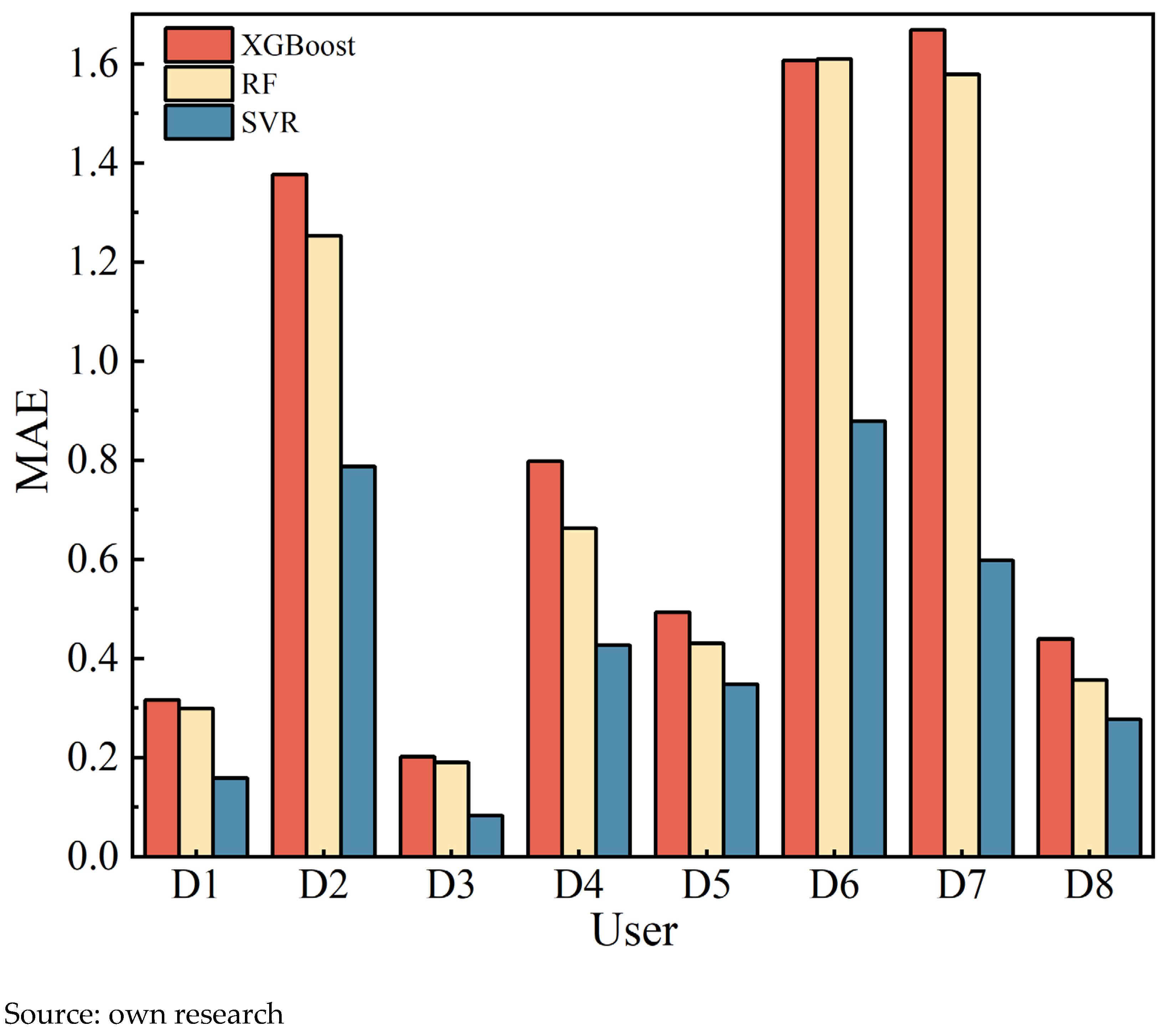
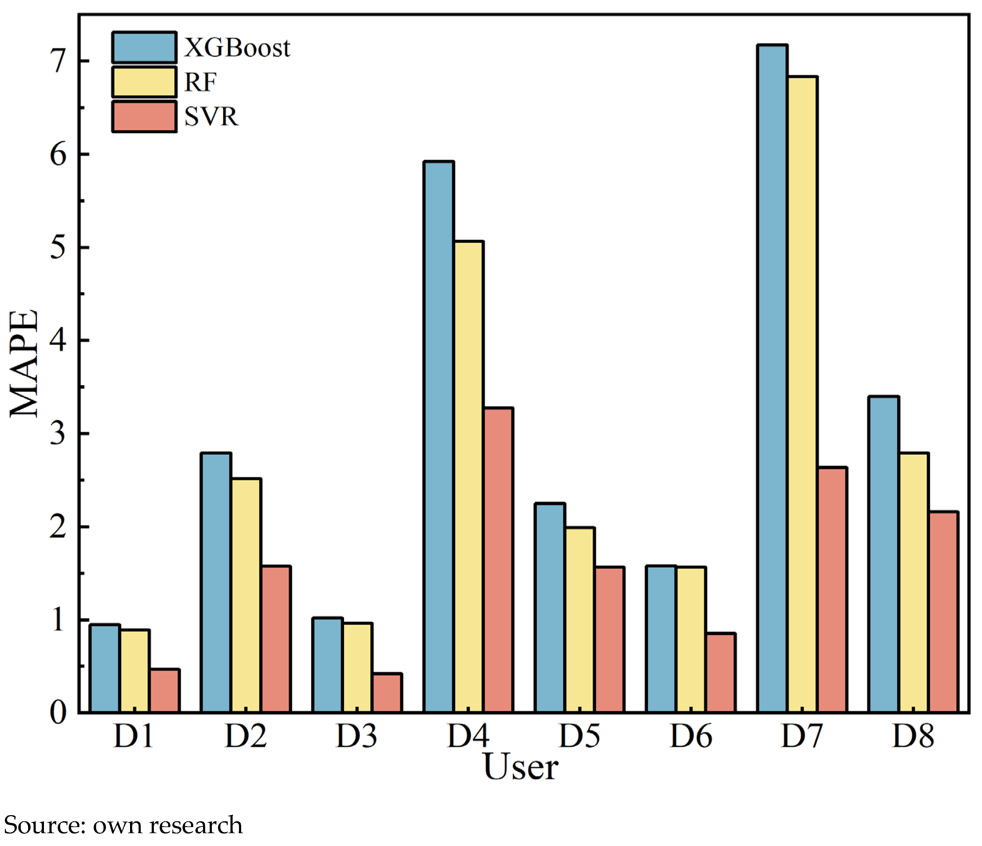
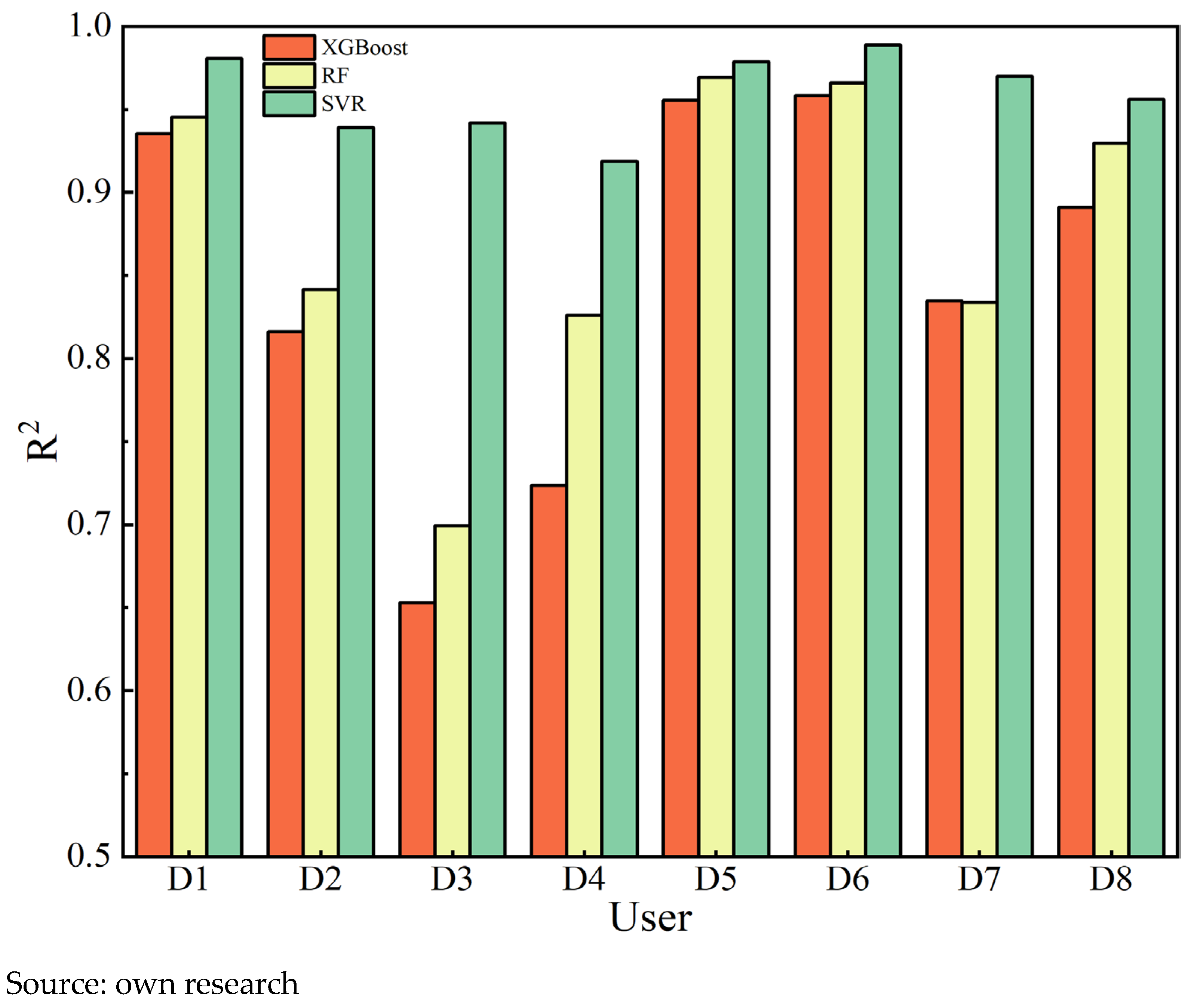
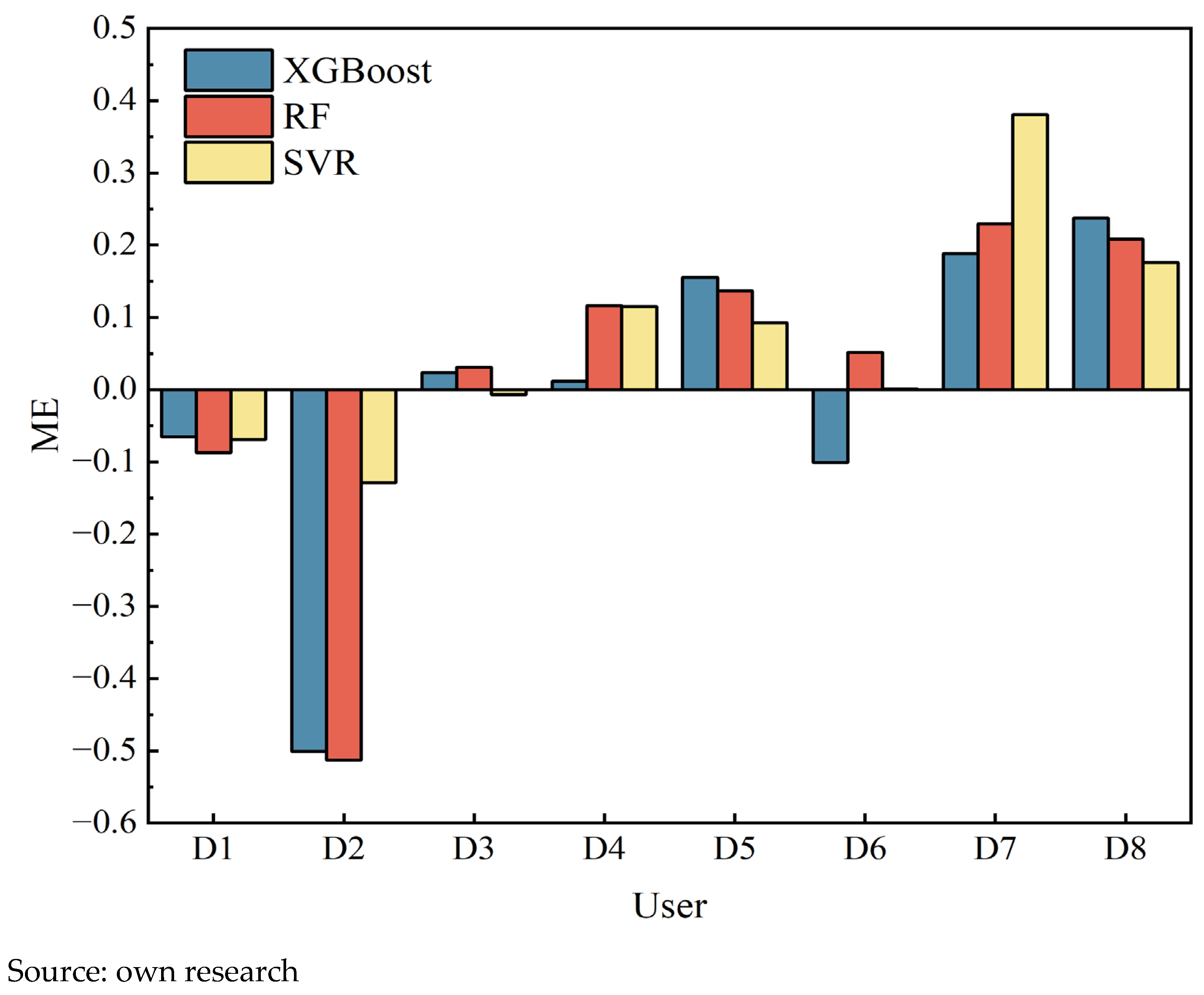
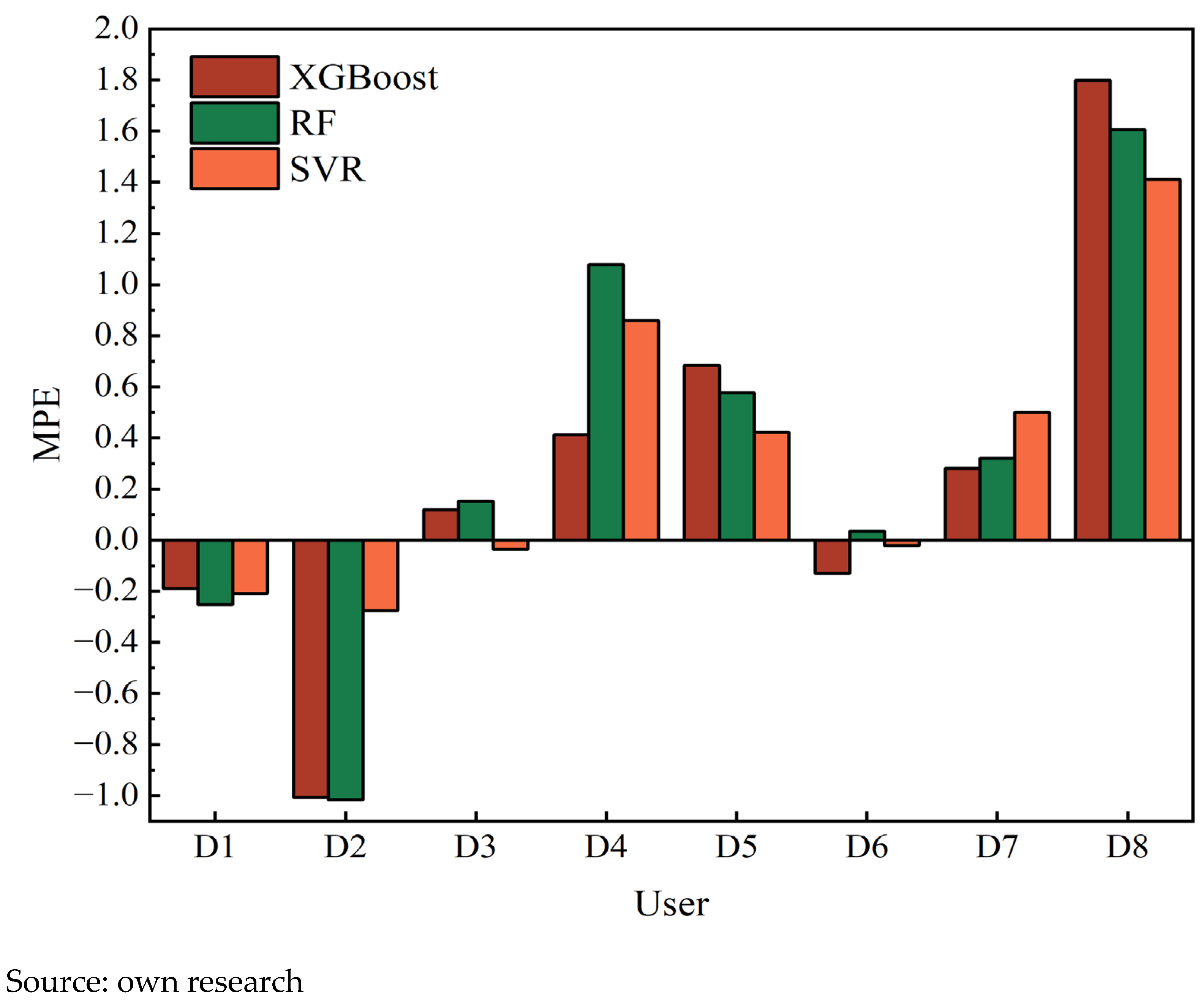
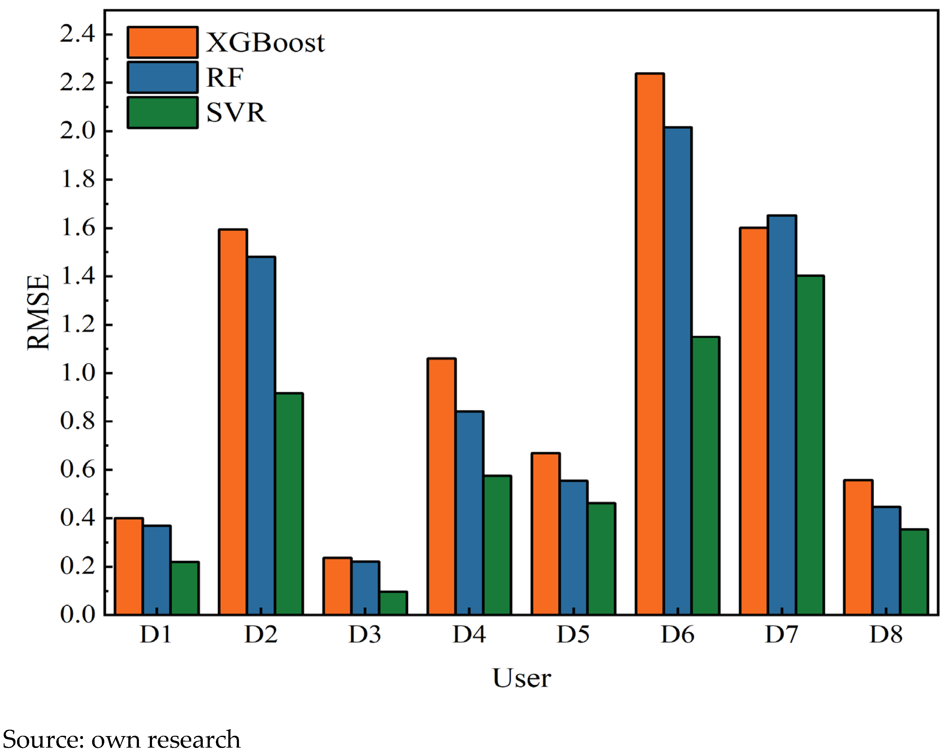
Given the forecasting task requires obtaining future natural gas demand for each user, the three selected forecasting models were trained based on the historical data of all users. After completing the model training, the performance of the three models was comprehensively calculated and compared across various evaluation metrics, with the results illustrated in Figure 6, Figure 7, Figure 8, Figure 9, Figure 10 and Figure 11.

According to the evaluation criteria for model performance metrics, lower values of MAE and MAPE indicate smaller prediction bias and higher accuracy, while an R² value closer to 1 reflects a better goodness-of-fit. For figures displaying error indicators (MAE, MAPE, RMSE, ME, and MPE), the Y-axis represents the absolute or percentage magnitude of the error. As shown in Figure 6, Figure 7, Figure 8, Figure 9, Figure 10 and Figure 11, in terms of ME and MPE, for some users, the SVR model did not exhibit the optimal performance. However, overall, it still significantly outperformed the XGBoost and RF models. In addition, the SVR model significantly outperforms both the XGBoost and RF in terms of MAE, MAPE and RMSE. Its R² value is also notably closer to 1, demonstrating comprehensively superior prediction performance and fitting effectiveness.

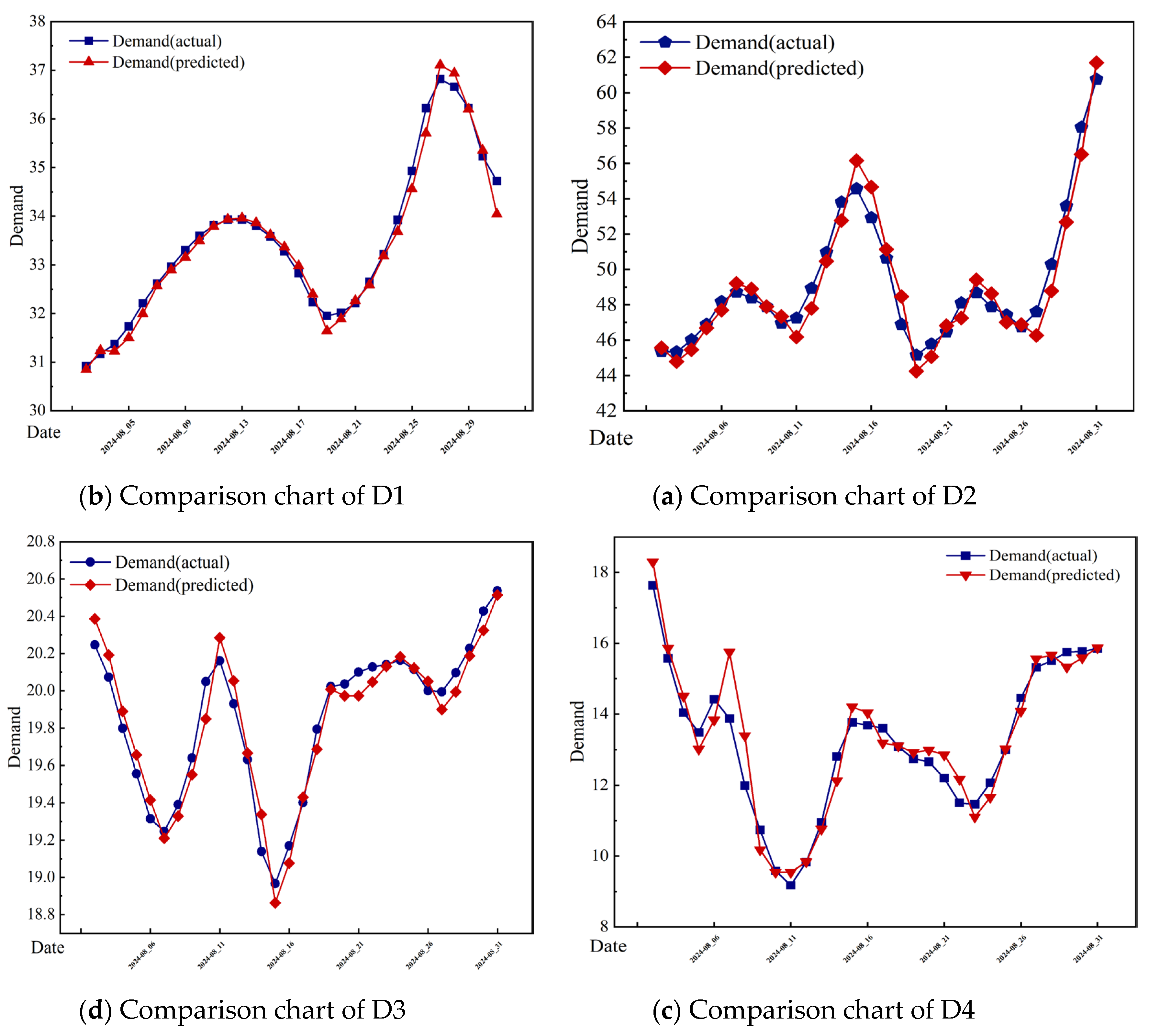
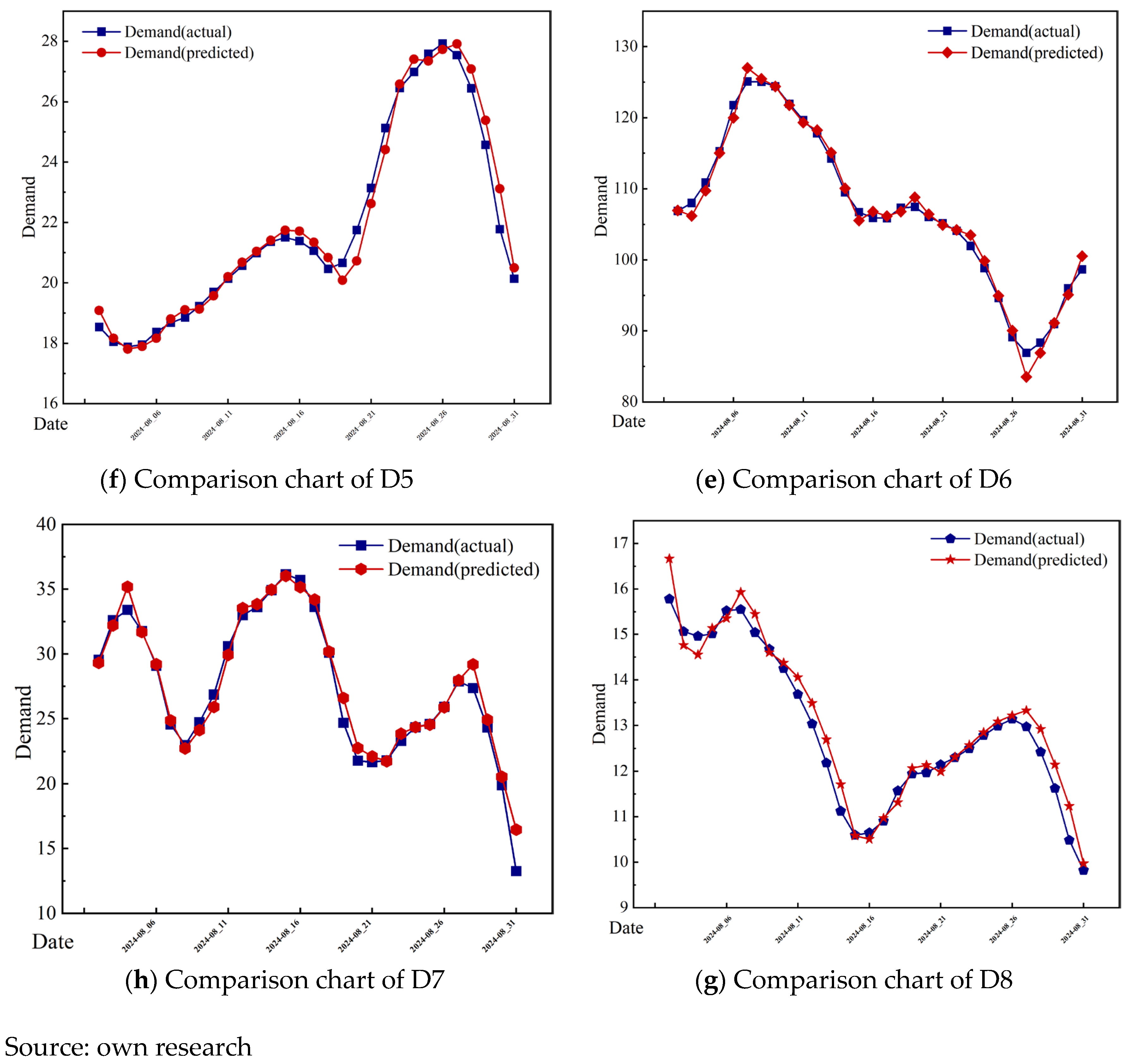
Based on the comprehensive evaluation of these three metrics, the SVR model was selected as the preferred forecasting model for subsequent analysis. To further visually demonstrate the training performance of the SVR model, the predicted values were compared against the actual values on the test set, with downstream users as the unit of analysis. The test set covers the period from 2 August to 31 August 2024. A detailed line chart comparing the predicted and actual values on the test set is presented in Figure 12.

It should be noted that the units of the Y-axis in Figure 12 is “10⁴ m³”. Based on the above, the SVR model was selected to forecast the natural gas demand for each user over the next month, generating daily demand predictions from 1 September 2024 to 30 September 2024.

3.3. Structure of Natural Gas Pipeline System

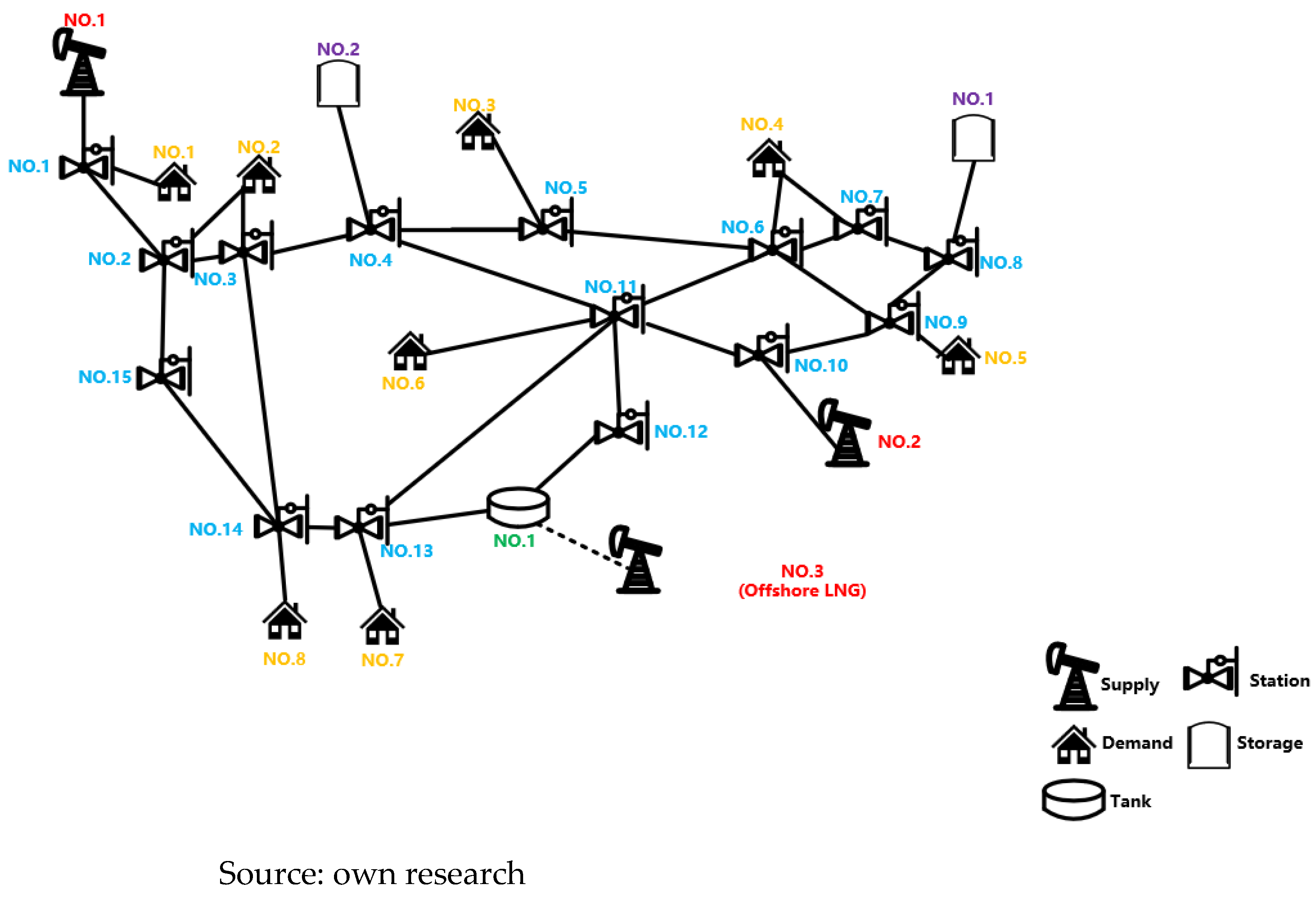
This section describes the pipeline network structure adopted in this study, whose topology is illustrated in Figure 13. The system comprises three gas sources, one LNG terminal, two gas storage facilities, eight end-users, and 37 pipelines. The specific parameters of each component are provided in Appendix A.

3.4. Case Study Scenario Setting

Based on the constraints set for each component in Section 3.3, the optimization model was solved with the objective of maximizing the operational economic efficiency of the natural gas industry chain. The operational results of key components in the model are presented in

Table 3. Optimized Daily Gas Supply Volume from Each Source.

Supply Code	Planned Supply (104 m3/d)	Supply Upper Limit (104 m3/d)	Price (RMB/m3)	Actual Gas Supply Volume (104 m3/d)
S1	115.0	120.0	1.5	120.0
S2	75.0	80.0	1.3	80.0
S3	65.0	70.0	1.6	48.0

Source: own research.

,

Table 4. Table of actual gas results obtained by users.

User Code	Planned Supply (104 m3/d)	Supply Lower Limit (104 m3/d)	Supply Upper Limit (104 m3/d)	Price (RMB/m3)	Actual Gas Volume (104 m3/d)
D1	37.0	22.2	37.0	4.3	25.0
D2	65.0	39.0	65.0	4.6	65.0
D3	21.0	12.6	21.0	4.6	21.0
D4	18.0	10.8	18.0	4.5	18.0
D5	21.0	12.6	21.0	4.4	21.0
D6	120.0	72.0	120.0	4.5	120.0
D7	33.0	19.8	33.0	4.7	33.0
D8	15.0	9.0	15.0	4.6	15.0

Source: own research.

,

Table 5. Table of pipeline actual gas transmission results.

Pipeline Code	Transportation Capacity Limit (104 m3/d)	Transportation Price (RMB/m3/km)	Actual Gas Transmission Volume of Pipelines (104 m3/d)
P1	120.0	101.1	95.0
P2	125.0	103.5	30.0
P3	115.0	110.2	0.0
P4	110.0	104.6	30.0
P5	100.0	106.5	0.0
P6	105.0	102.6	39.0
P7	110.0	94.7	21.0
P8	105.0	110.5	18.0
P9	120.0	100.6	0.0
P10	120.0	90.9	0.0
P11	130.0	109.4	0.0
P12	125.0	80.2	0.0
P13	115.0	103.9	40.0
P14	125.0	110.5	19.0
P15	125.0	88.2	99.0
P16	100.0	110.4	0.0
P17	110.0	106.5	0.0
P18	105.0	103.5	15.0
P19	120.0	108.7	0.0

Source: own research.

,

Table 6. Table of actual gas withdrawal volume of storage.

Storage Code	Planned Gas Withdrawal Volume (104 m3/d)	Gas Withdrawal Capacity Limit (104 m3/d)	Gas Withdrawal Price (RMB/m3)	Actual Gas Withdrawal Volume (104 m3/d)
K1	15.0	40.0	0.3	40.0
K2	15.0	30.0	0.1	30.0

Source: own research.

and

Table 7. Table of actual LNG export volume of LNG terminal.

LNG Terminal Code	Planned LNG Export Volume (104 m3/d)	LNG Export Capacity Limit (104 m3/d)	LNG Export Price (RMB/m3)	Actual LNG Export Volume (104 m3/d)
T1	50.0	90.0	0.2	48.0

Source: own research.

.

This table presents the optimized daily gas supply volume from each upstream source. The results indicate that Source 1 and Source 2 operate consistently at their maximum supply capacities of 1.20 million m³/day and 0.80 million m³/day, respectively. This suggests their economic superiority, likely due to lower procurement costs, making them the primary baseload suppliers in the optimized strategy. In contrast, the supply from Source 3 varies dynamically between 0.07 and 0.46 million m³/day, fulfilling a peaking role to balance fluctuations in downstream demand.

This table details the allocated daily natural gas volume received by each downstream user. The optimization model consistently allocates volumes at the maximum demand upper limit for all users except D1, a strategy directly aimed at maximizing sales revenue. Furthermore, it is confirmed that the operational constraint—which guarantees a minimum supply of 60% of the upper limit for each user—is strictly adhered to, ensuring supply security and stability even under the profit-maximization objective.

This table summarizes the optimized flow volumes within each pipeline in the network. The results empirically validate the model’s dynamic routing strategy, which proactively selects cost-efficient pathways and avoids those with high transportation fees. The flow distribution is not uniform but is strategically allocated to minimize the total transportation cost across the system, a critical factor in enhancing the overall net profit of the industrial chain.

This table shows the optimized withdrawal volumes from the gas storage facilities. The operation of these facilities is strategically coordinated, likely in conjunction with the output of S3, to act as a buffering and peak-shaving mechanism. By injecting during low-demand periods and withdrawing during high-demand periods, the storage facilities enhance the system’s flexibility, thereby supporting a stable supply to downstream users and contributing to the overall economic efficiency.

This table indicates the optimized daily send-out volume from the LNG terminal. Similarly to the primary gas sources S1 and S2, the LNG terminal operates at or near its full capacity throughout the optimization period. This confirms its role as a stable, reliable, and economically viable supply source within the multi-source portfolio optimized by the model to maximize overall profitability.

Based on the results presented in the aforementioned tables, the optimized strategy of the model exhibits the following characteristics to maximize the economic efficiency of the industrial chain: with the exception of the first user, the gas supply allocated to all other users is set to their maximum demand upper limits, thereby maximizing downstream natural gas sales revenue. Meanwhile, to ensure reliable downstream supply, the gas sources, storage facilities, and the LNG terminal are all operating near their maximum supply capacities.

It is noteworthy that, under the objective of maximizing operational economic profit (as defined in Equation (12)), the pipeline network optimization model adopts a dynamic route selection strategy to proactively avoid pipelines with high marginal costs and inefficient transportation paths, which objectively reduces overall pipeline transportation costs.

Under this optimized strategy, the total downstream natural gas sales revenue reaches 14.53 million yuan, the total resource supply cost of the industrial chain is 3.61 million yuan, and the total pipeline transportation cost is 0.41 million yuan, resulting in a net profit of 10.88 million yuan for the industrial chain. In summary, the operational results of the model align closely with actual conditions, demonstrating its applicability and effectiveness in evaluating the profitability of future gas supply strategies.

3.5. Simulation of Future Gas Supply Revenue Scenarios

Based on the forecasted natural gas demand of downstream users for the upcoming month obtained in Section 3.2, the results were used as input parameters for the optimization model. Through model computation, the actual daily supply volume from each upstream gas source and the actual received volume for each downstream user over the next month were derived. Corresponding natural gas sales revenue was also calculated accordingly. This process laid a data foundation for further in-depth analysis of gas supply conditions, user receipt details, and fluctuation trends in economic indicators of the industrial chain.

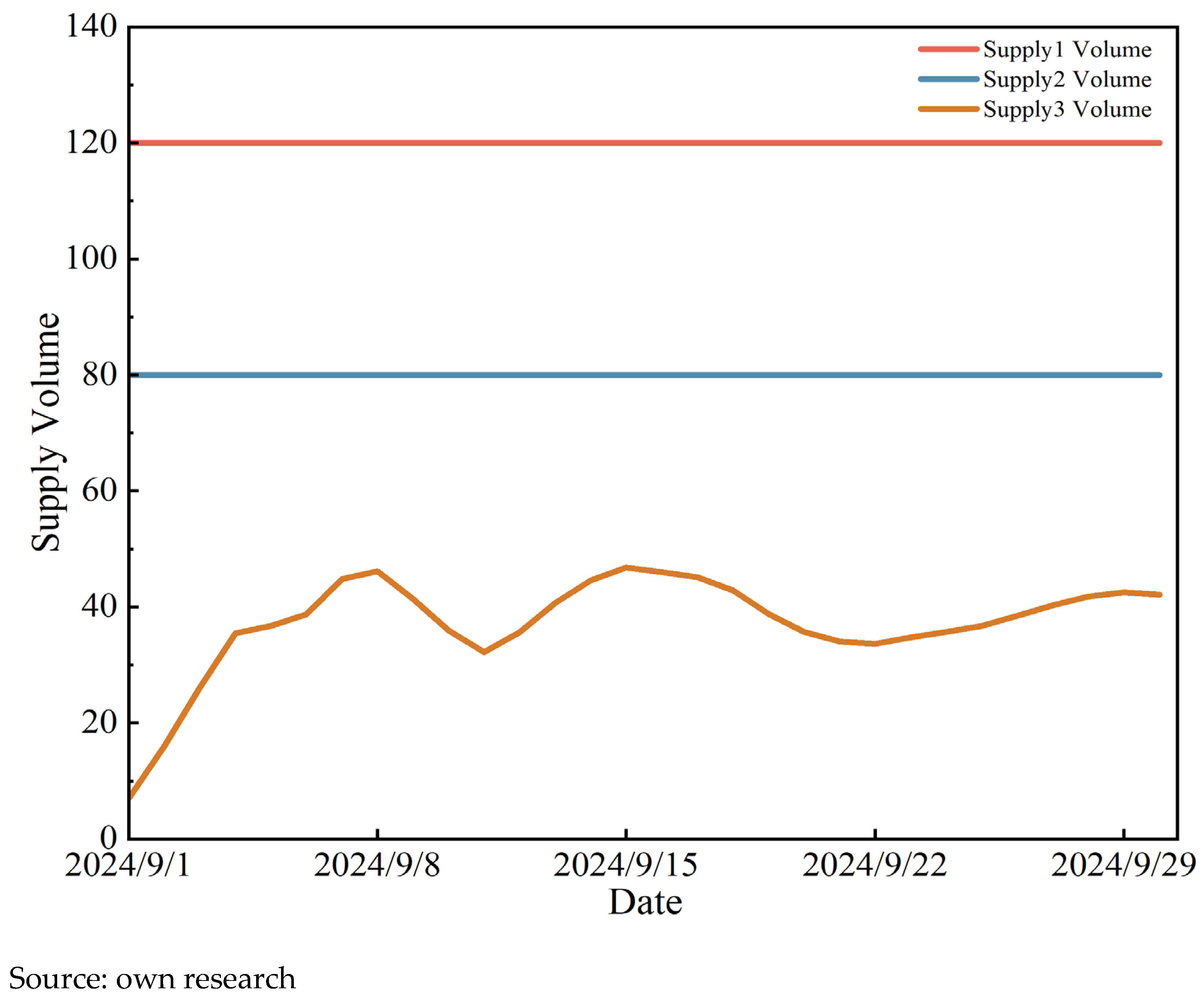
According to the model results, the actual gas supply from Source 1 and Source 2 remained constant at their supply upper limits of 1.20 million m³/day and 0.80 million m³/day, respectively, throughout the forecast month, indicating that both sources operated at full capacity during the entire period. In contrast, the supply from Source 3 varied dynamically between 0.07 million m³/day and 0.46 million m³/day, with an average supply of 0.36 million m³/day. The daily variation in gas supply from each source is illustrated in Figure 14. These results demonstrate that, in response to differentiated demand among downstream market users, the model achieved an overall supply–demand balance in the natural gas industry chain by dynamically adjusting the output of Source 3.

A further comparison of the gas supply distribution between the model training phase and the forecasting phase reveals a consistent operational pattern among the three gas sources: S1 and S2, as the primary supply sources, maintain high output levels, while S3 serves a load-following role to accommodate fluctuations. This consistency demonstrates the model’s strong generalization capability and stability, enabling it to accurately simulate the supply characteristics of the natural gas industry chain across different temporal windows. It thereby provides a reliable basis for subsequent economic benefit calculations and gas supply strategy formulation.

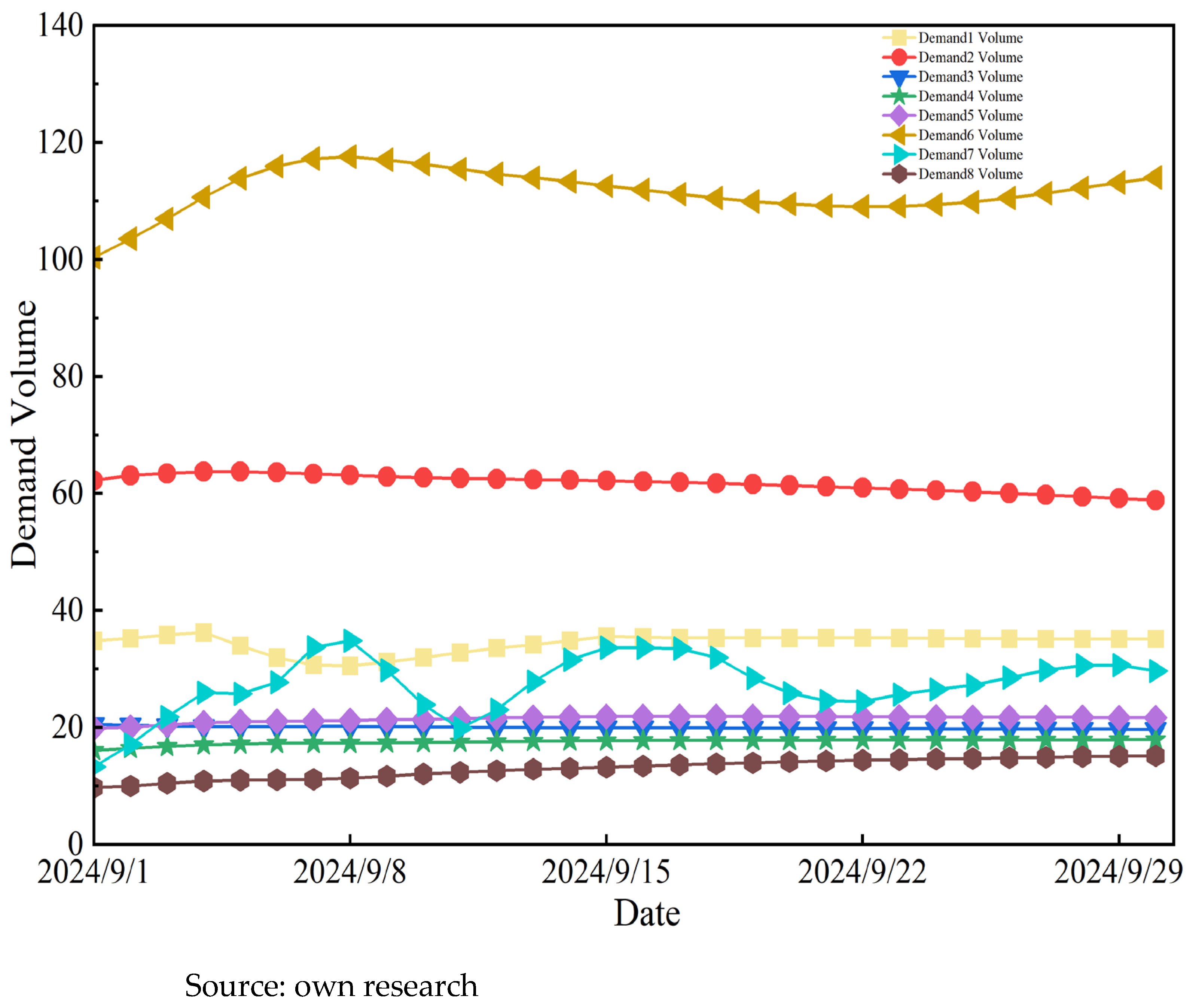
As shown in Figure 15, the variation in actual gas receipt by downstream market users over the upcoming month—calculated by the model—is presented in units of 10⁴ m³. Further analysis of user gas receipts reveals that User 1, User 2, User 6, and User 7 are key downstream consumers, accounting for 13.0%, 23.6%, 42.7%, and 10.5% of the total supply, respectively. Among them, User 6 serves as the dominant consumer, with a peak daily receipt reaching 1.17 million m³, while User 2 is a stable high-load user, both of which require particular attention in gas supply strategy formulation. Meanwhile, User 7 exhibits significant fluctuations in gas receipt, ranging from 0.13 million m³/day to 0.35 million m³/day. The daily gas receipts of the remaining users remained relatively stable.

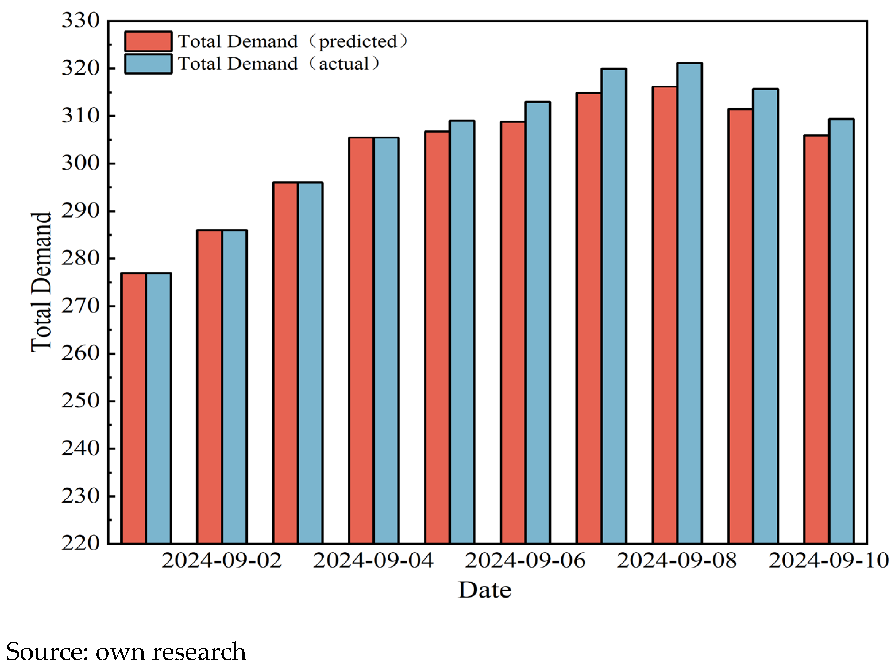
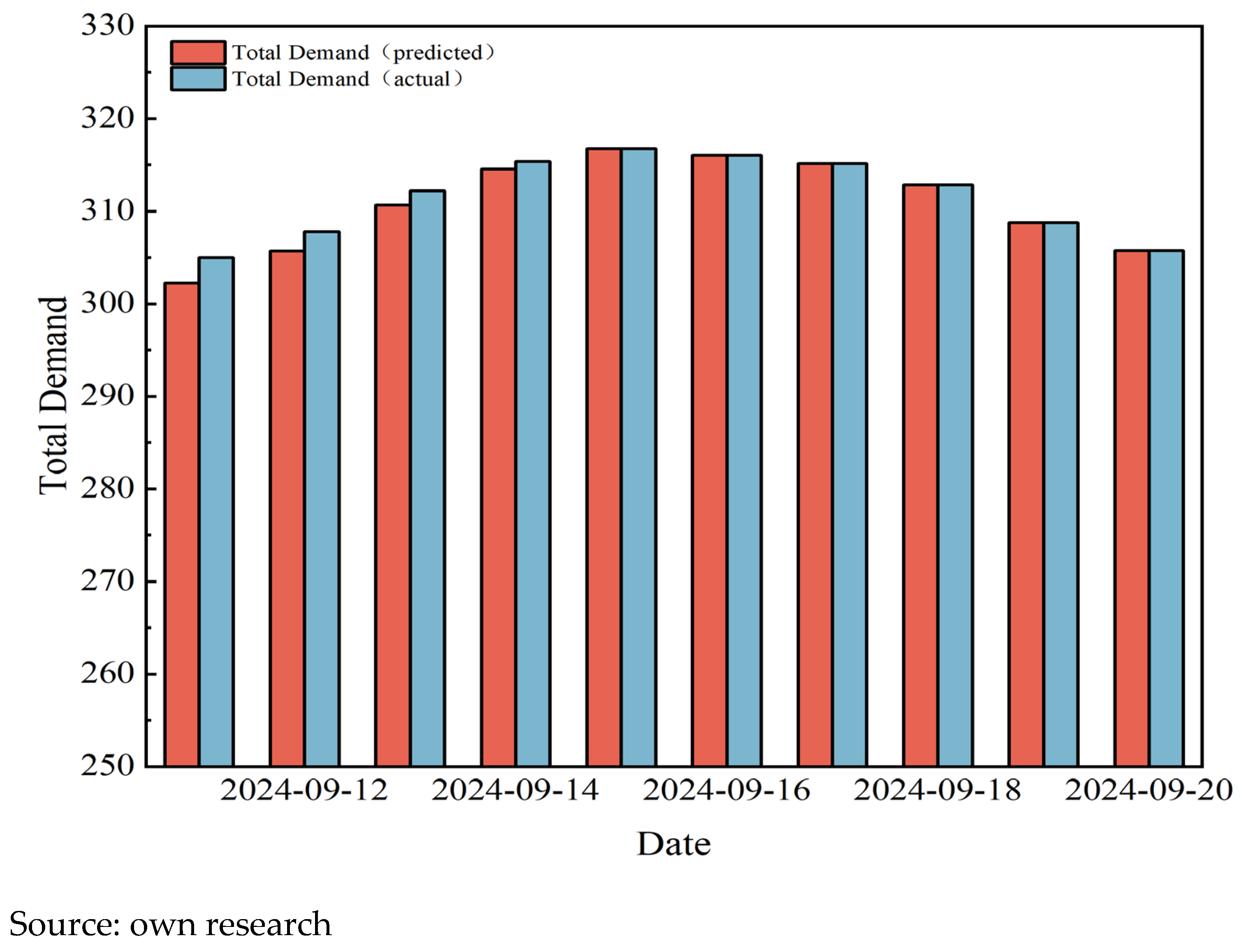
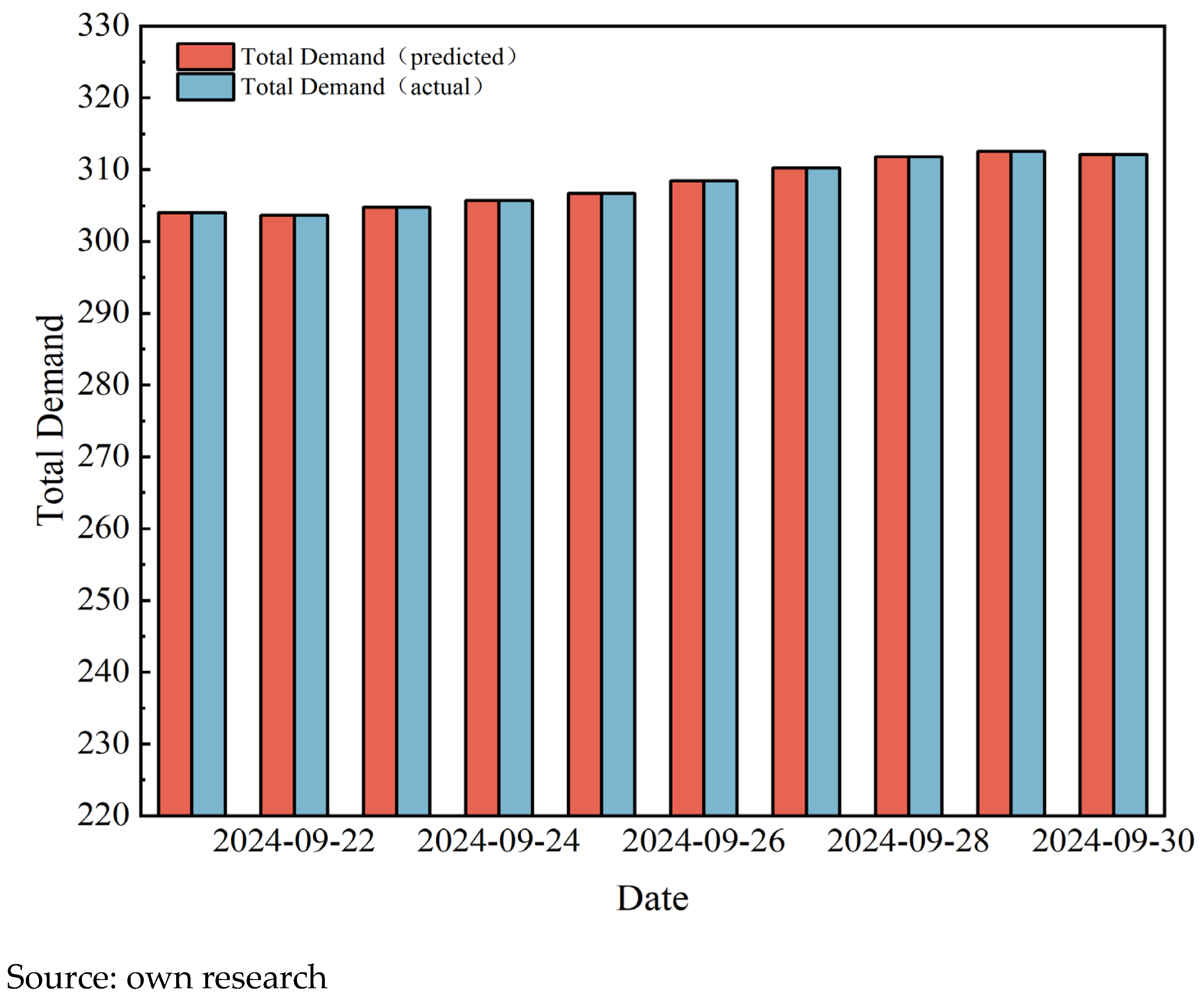
To further illustrate the overall fulfillment of downstream user demand, the forecasted total daily demand of downstream users for the upcoming month is compared with the total actual gas supply volume after optimization by the model. This comparison assists operational personnel in quickly identifying potential short-term supply shortfalls. The comparative results are shown in Figure 16, Figure 17 and Figure 18.

As shown in Figure 16, Figure 17 and Figure 18, varying degrees of supply shortfalls are observed between 5 September and 14 September, which require attention from relevant operational personnel to adjust corresponding gas supply strategies while ensuring economic benefits of the industrial chain.

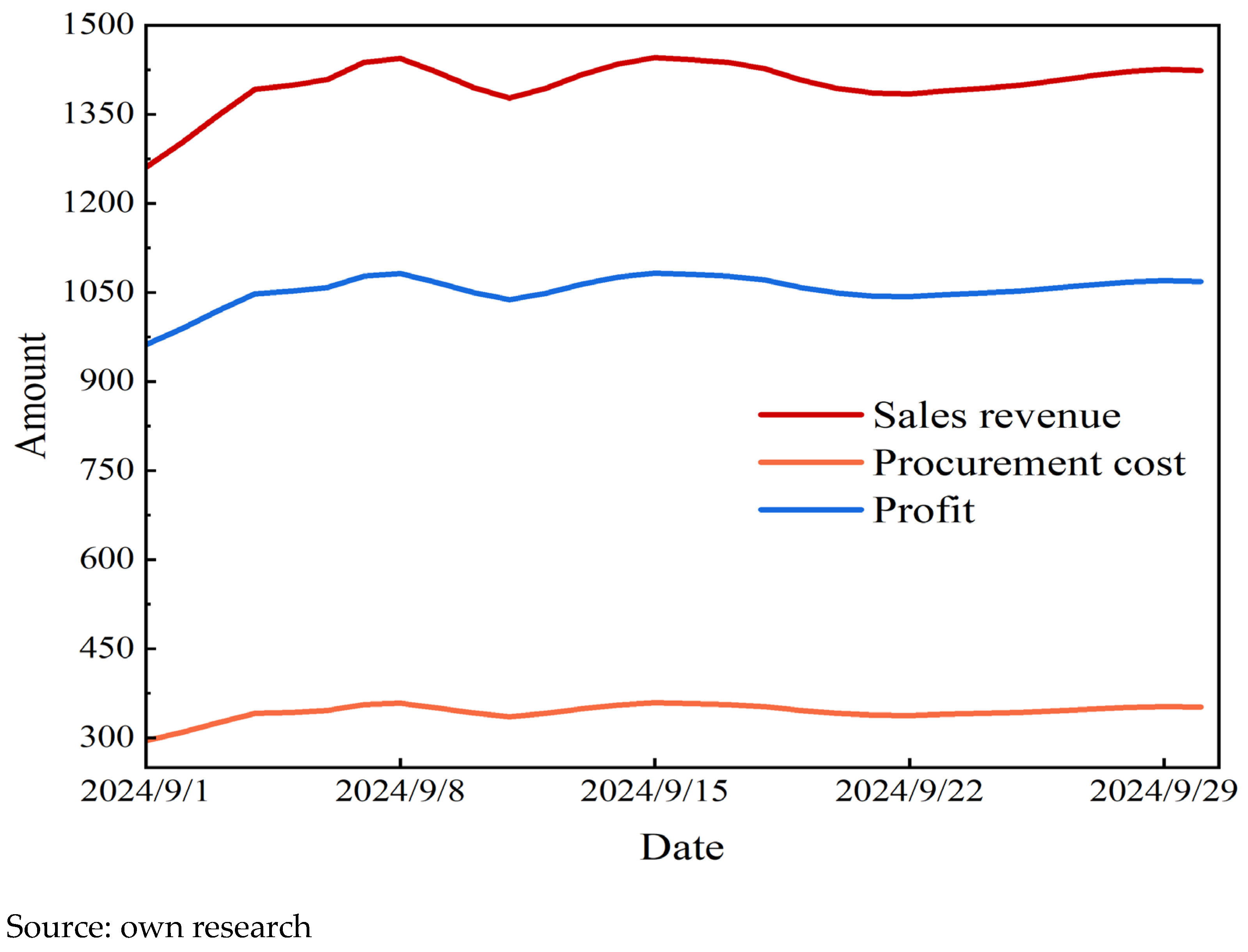
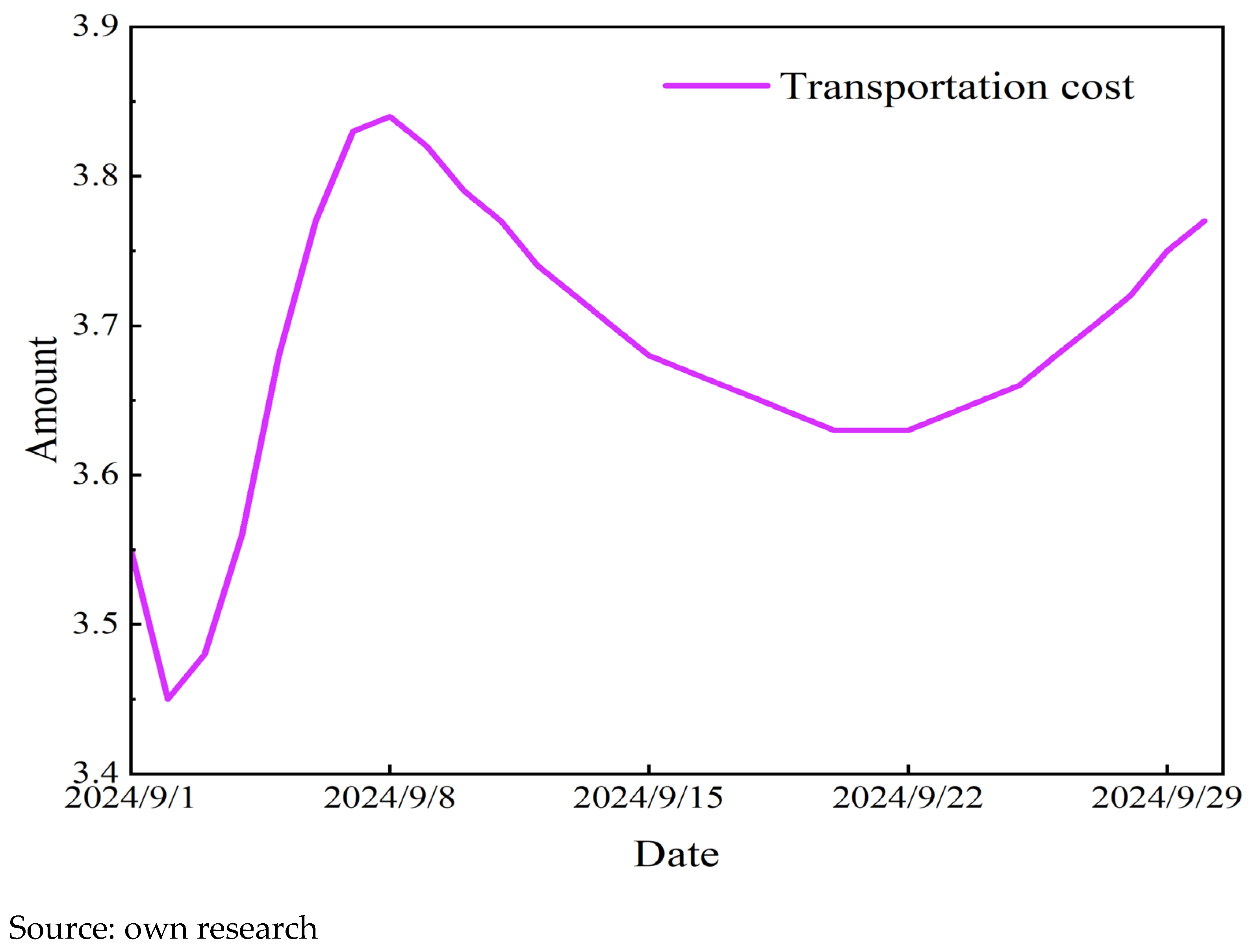
Based on the actual gas supply volumes obtained from model simulations using forecasted inputs, the variations in economic indicators of the natural gas industry chain over the upcoming month were calculated, as shown in Figure 19 and Figure 20. During this period, the average daily downstream sales revenue was 13.98 million yuan, fluctuating between 12.61 million yuan and 14.45 million yuan. The average daily total resource cost was approximately 3.46 million yuan, ranging from 2.95 million yuan to 3.59 million yuan. The total pipeline transportation cost remained relatively stable, averaging about 37,000 yuan per day, with a maximum of 38,000 yuan and a minimum of 34,000 yuan.

In terms of the operational economic profit of the entire industry chain, the average daily value reached 10.57 million yuan. The highest profit, 10.83 million yuan, occurred on 15 September, while the lowest, 9.62 million yuan, was recorded on 1 September. All economic indicators showed a gradual upward trend from the beginning to the middle of the month, followed by a slight decline thereafter, though overall fluctuations remained within a controllable range.

The economic results presented in Figure 16, showing a significant margin between total revenue and total costs, warrant further discussion regarding market structure. The reviewer’s observation on the profit-to-cost ratio is accurate. However, this result is a direct consequence of the model’s fundamental economic assumptions and should not be construed as simulating a monopolistic market.

It should be noted that due to the significantly smaller magnitude of pipeline transportation costs compared to other economic indicators, their variations are presented separately.

The results clearly demonstrate the economic performance of the natural gas industry chain under given supply and demand conditions, providing data-driven support for the formulation of future gas supply strategies.

4. Conclusions

This paper focuses on economic performance, developing an optimization model for the industrial chain economic returns based on variations in natural gas demand from downstream market users. To quantify the profitability of the industrial chain under specific supply–demand scenarios, the model uses historical operational data as a baseline and reconstructs a high-quality benchmark dataset through temporal intersection screening and wavelet denoising techniques. This dataset provides a reliable foundation for subsequent natural gas demand forecasting tasks.

Based on the established high-quality benchmark dataset, this study systematically evaluated the performance of three forecasting models. The data partitioning strategy adopted utilized the last month of the dataset as the test set, with the remainder serving as the training set. After completing model training, the predictions on the test set were comprehensively compared against actual values by calculating three key performance metrics—MAE, MAPE, and R²—to thoroughly assess the prediction accuracy and robustness of each model. Through this evaluation, the Support Vector Regression (SVR) model was identified as the optimal forecasting method. Finally, using the last month of historical data as input, the selected SVR model was applied to forecast the specific natural gas demand for the upcoming month.

Upon obtaining the forecasted natural gas demand, it was treated as the actual downstream user demand for the upcoming month. A pipeline network topology was then constructed, with operational parameters and physical and operational constraints defined for its core components. The objective function was set to maximize the operational economic efficiency of the industrial chain, forming a comprehensive natural gas supply chain optimization model. Based on historical operational data, key parameters such as gas transportation volumes were scientifically configured to ensure the model’s outputs align with real-world conditions. Finally, using the forecasted demand values as inputs, the optimization model was computed to derive the economic performance of the industrial chain under specific future supply–demand scenarios.

The results of this case study demonstrate that, within a specific natural gas transmission and distribution network topology combined with user demand profiles, the economic performance of the entire industrial chain can be quantitatively evaluated. This method can be effectively applied in engineering practice. Under conventional operating conditions, maximizing operational economic efficiency is the primary objective for natural gas industrial chain enterprises. Operational personnel can use this model by inputting proposed supply strategies to preliminarily estimate the resulting corporate profitability. The evaluation outcomes can, to a certain extent, reflect the rationality of the strategy, thereby guiding companies to dynamically adjust resource allocation while ensuring secure and stable supply across the industrial chain, ultimately achieving optimized economic performance.

However, the proposed model still has certain limitations and areas for improvement, which are outlined as follows:

(1) The natural gas demand of downstream market users is a complex variable influenced by the coupling effects of multiple factors. However, during data processing in this study, it was treated solely as a time series input to the forecasting model, without considering influencing factors such as temperature and holidays. As a result, the obtained data may deviate from actual conditions.

(2) This paper primarily focused on forecasting demand for the upcoming month, addressing short-term supply situations, and did not extend to long-term strategy formulation. The analytical perspective was thus limited to a monthly scale. However, since enterprise planning typically encompasses short, medium, and long-term dimensions, the limited consideration given to medium- and long-term strategic aspects remains a constraint in serving corporate objectives comprehensively.

(3) The pipeline network topology constructed in this study is relatively oversimplified, making the model insufficient for meeting the computational requirements of diverse structural configurations. For large-scale and complex natural gas pipeline networks, this model cannot accurately estimate economic performance based solely on user demand.

(4) The current research is based on the premise of normal operation of the natural gas industry chain and does not consider its performance and economic returns under special conditions such as gas source failures or pipeline leaks. Meanwhile, the design of the model’s objective function is primarily economically oriented, lacking consideration for differences in operational goals across various scenarios. Future work should incorporate diverse operating conditions and establish differentiated objective functions based on the priority of operational goals in the natural gas industry chain, so as to enhance the model’s applicability and decision-support value in complex environments.

Regarding the aforementioned limitations, the following improvement approaches are suggested:

(1) During the initial screening of forecasting models, priority should be given to those demonstrating superior regression prediction performance. When processing the collected initial data, factors such as temperature should be incorporated to construct a fully integrated natural gas demand forecasting model that accounts for multiple influencing factors.

(2) Building on the full consideration of multiple influencing factors, forecasting should be conducted across different time spans, with temporal scales set to weeks, months, and years, respectively, to align with the multi-level decision-making perspectives required by natural gas industry chain enterprises in strategy formulation.

(3) Based on the existing pipeline network structure, key facilities such as gas sources, consumers, and storage facilities should be appropriately expanded, and the gas supply paths for consumers should be complexified to form a more looped network configuration. Meanwhile, additional constraints should be incorporated into pipeline components to increase the computational complexity of the model, enabling it to better adapt to diversified and complex pipeline structures.

(4) On the premise that the optimization model can meet normal operating conditions, simulations of critical facility failure scenarios should be introduced. For failure conditions, the objective function should be formulated as a coupled function combining “maximizing the operational economic efficiency of the natural gas industry chain” and “ensuring downstream gas supply security,” so as to enhance the model’s adaptability and rationality in practical operations.

(5) Introduce advanced methods for handling uncertainties to enhance the robustness and practicality of the model. Specifically, this includes: ① Quantifying Forecast Uncertainty: Using methods like Quantile Regression Forests or Bayesian SVR to generate prediction intervals instead of point forecasts. ② Implementing Robust Optimization: Reformulating the model using a robust optimization framework where the demand parameter is an uncertain variable within a predefined uncertainty set. This would immunize the solution against demand fluctuations within that range. ③ Stochastic Programming: Formulating a two-stage stochastic program where the first-stage decisions are made before demand is known, and second-stage recourse actions are taken after demand is realized.