Article

An Improved Regularization Stochastic Configuration Network for Robust Wind Speed Prediction

1
State Grid Liaoning Province Electric Power Co., Ltd., Fuxin Power Supply Company, Fuxin 123000, China
2
Faculty of Electrical and Control Engineering, Liaoning Technical University, Huludao 125105, China
*
Author to whom correspondence should be addressed.
Energies 2025, 18(23), 6170; https://doi.org/10.3390/en18236170
Submission received: 4 September 2025 / Revised: 28 October 2025 / Accepted: 5 November 2025 / Published: 25 November 2025
(This article belongs to the Section A3: Wind, Wave and Tidal Energy)

Abstract

To address the limitations of Stochastic Configured Networks (SCNs) in wind speed prediction, specifically insufficient regularization capability and a high risk of overfitting, this paper proposes a novel Regularized Stochastic Configured Network (RSCN). By integrating L1 and L2 regularization techniques from Elastic Net, RSCNs achieve feature sparsity while preserving prediction accuracy. Furthermore, a dynamic loss coefficient and a penalty term based on historical training loss are introduced to adaptively modulate the regularization strength during model training. Experimental results demonstrate that RSCNs achieve superior prediction performance and enhanced stability across four benchmark regression datasets and two real-world wind speed datasets. Compared with conventional SCNs and the swarm intelligence optimization-based variant HPO-SCNs, RSCNs significantly reduce the performance gap between training and test sets while maintaining high predictive accuracy. On average, improvements in R 2 , MAE, and RMSE exceed 50% reduction in error discrepancies. The proposed method offers an effective solution for wind power forecasting by effectively balancing generalization ability and computational efficiency, thereby holding practical significance for real-world applications.

1. Introduction

Renewable energy system prediction is increasingly being adopted in industrial applications [1,2]. Accurate wind speed prediction methods are therefore essential to support the large-scale integration of wind power into energy systems. However, meteorological variables such as wind speed and direction exhibit inherent randomness [3,4], often characterized by strong nonlinearity. Furthermore, practical data acquisition challenges—such as sensor malfunctions—introduce noise and missing values into wind power datasets, resulting in intermittent and highly fluctuating wind speed profiles. Despite these challenges, wind speed data possess distinct temporal dependencies and underlying patterns [5], which enable neural network models to learn multi-scale features and perform effective predictions. Nevertheless, current wind speed prediction models still achieve suboptimal performance across key evaluation metrics. While small MAE (Mean Absolute Error) values may suggest acceptable average accuracy, significant RMSE (Root Mean Square Error) fluctuations reveal high sensitivity to outlier predictions. The accumulation of such errors compromises prediction stability and restricts model reliability in real-world engineering scenarios. More importantly, most existing approaches emphasize localized parameter tuning, with insufficient focus on holistic optimization of global model performance. For instance, fixed regularization parameters fail to adapt dynamically to the temporal non-stationarity and spatial heterogeneity prevalent in wind speed data, while stage-wise regularization strategies may induce performance imbalances across different phases of training.
Supervised learning algorithms can overcome the limitations of local learning and the low accuracy associated with global learning [6,7]. In 2017, Wang and Li [8] introduced a reliable stochastic learning framework through a novel supervisory mechanism, termed Stochastic Configuration Networks (SCNs). The interpretability and universal approximation capability of SCNs have attracted extensive research interest for various industrial applications. For instance, Li and Wang [9] proposed a two-dimensional convolutional stochastic configuration network for image processing tasks. Zhou et al. [10] extended Greedy SCNs (GSCNs) into a deep architecture, improving prediction accuracy and stability for high-dimensional and large-scale data by incorporating negative correlation learning [11]. Building upon Recurrent Stochastic Configuration Networks [12], Dang and Wang [13] integrated the Takagi-Sugeno-Kang fuzzy reasoning system into SCNs to handle uncertainties during model construction. Sun et al. [14] combined SCNs with dynamic forgetting factor sliding window technology to develop an online-updated soft sensor, effectively addressing data drift in semi-autonomous ball mill crusher systems. Han et al. [15] addressed the challenge of manual hyperparameter tuning by reconstructing the generation method of random scale factors using a cloud model. Li et al. [16] developed a robust stochastic configuration network based on the maximum entropy criterion, enhancing performance in regression tasks under significant noise or outlier contamination. In 2019, Wu et al. [17] proposed MoGL-SCN, a Bayesian framework-based robust SCN that employs a mixture of Gaussian and Laplace distributions. Subsequently, Wu et al. [18] abandoned the original incremental structure and instead generated node parameters directly using an improved sparrow search algorithm. Han et al. [19] introduced an adaptive input weight and bias configuration method based on adaptive inertia weight, termed Adaptive Weighted Stochastic Configuration Network (AWSCN), which dynamically adjusts node parameters to minimize residuals. Dai et al. [20] enhanced SCNs by incorporating a class balancer to address imbalanced datasets and adopted a fast recursive algorithm for output weight updates, resulting in an approach named Imbalanced Learning for SCNs (IL-SCN).
Although the aforementioned studies have improved the performance of SCNs in various aspects, they have not sufficiently addressed enhancing the model’s regularization capability to mitigate overfitting risks in the later stages of training and prediction. With regard to regularization techniques for SCNs, Zhao et al. [21] proposed L2-regularized SCNs in 2020, while Pan et al. [22] introduced manifold-regularized SCNs in 2021. These methods achieve regularization by incorporating L2 norms into the supervisory mechanism or embedding manifold constraints, thereby partially reducing overfitting tendencies. However, these approaches overlook two critical limitations: first, they fail to effectively balance feature sparsity and model stability; second, they do not account for the dynamically evolving regularization requirements during the incremental construction of the network. To address these shortcomings, this paper proposes a novel regularization framework. First, Elastic Net is employed to jointly integrate L1 and L2 regularization terms, harnessing the complementary advantages of sparsity induction and coefficient shrinkage. Second, a dynamic constraint coefficient z, derived from historical loss values, is introduced to enable adaptive modulation of regularization strength throughout the learning process. The main contributions of this work are summarized as follows:
(1)
The Elastic Net framework, which integrates L1 and L2 regularization techniques, is incorporated into SCNs. This integration enables the model to produce sparse solutions while maintaining a high level of prediction accuracy, thereby enhancing its suitability for feature selection. Furthermore, the approach effectively controls model complexity and mitigates the risk of overfitting.
(2)
A dynamic loss coefficient, derived from historical loss values, is introduced to enable adaptive adjustment of the model’s regularization intensity, and a penalty term based on both the historical error and the contribution of newly added nodes is incorporated to fine-tune the regularization strength.
The remainder of this paper is organized as follows. Section 2 presents a detailed description of the model principles, along with the fundamental concepts of L1 and L2 regularization; Section 3 elaborates on the proposed improvement methods and their specific details; Section 4 provides an in-depth discussion of the performance evaluation experiments; Finally, Section 5 summarizes the main contributions of this article.

2. Materials and Methods

2.1. Stochastic Configuration Networks

In SCNs [8], let there be actual values Y, model calculation results f j 1 ( X ) , and an activation function g. Assuming a tensor space Γ that is dense under the L 2 norm, there exists a constant b g such that 0 < g < b g for all g Γ . Furthermore, given a real number r ( 0 , 1 ) and a sequence of non-negative real numbers { μ L } .
Taking the jth node as an example, as the number of nodes increases, the input weights w j and input bias b j are randomly generated within a random scale factor λ .
w j = λ × ( 2 × rand ( d , L ) 1 )
b j = λ × ( 2 × rand ( 1 , L ) 1 )
The generated weights and biases are subsequently evaluated by the supervisory mechanism to determine whether they meet the conditions, specifically whether the output g j ( X ) and residual e L 1 ( X ) of the hidden layer composed of w j and b j satisfy (5).
g j ( X ) = g w j · X + b j
e j 1 ( X ) = Y f j 1 ( X )
e L 1 ( X ) , g ( X ) 2 b g 2 δ j , q q = 1 , 2 , , K
When the aforementioned conditions are satisfied, the output weight is computed, and the result is subsequently produced.

2.2. L1 and L2 Regularization

To address the issue of large generalization errors caused by model overfitting, L1 or L2 regularization techniques are commonly employed [23,24,25,26]. The L1 and L2 norms are defined as follows:
m 1 = m 1 + m 2 + + m n
m 2 = m 1 2 + m 2 2 + + m n 2
For a vector m , the L1 norm represents the Manhattan Distance of its elements, while the L2 norm represents the Euclidean Distance of its elements. The core idea of L1 regularization is to introduce an L1 penalty term that drives the model weights toward zero, thereby enabling sparse feature learning, reducing model complexity, and enhancing model generalization. Similarly, L2 regularization introduces an L2 penalty term into gradient descent, incorporating a weight minimization objective. This simultaneously minimizes the sum of squared weights and the training error, effectively preventing gradient explosion caused by excessively large weights.

3. RSCNs

3.1. Elastic Networks Combine L1 and L2 Regularization

For Elastic Net regularization [27], the objective function under the resilient regularization constraint is formulated as follows:
min e r r o r 2 2 + l 1 m 1 + l 2 m 2
where e r r o r denotes the prediction error and l 1 and l 2 represent the constraint coefficients. However, to incorporate it into the supervision mechanism of SCNs, the original constraint in (5) is first analyzed, a new variable k s i is introduced, and the left-hand side of the equation is normalized, yielding
k s i = e L 1 ( X ) , g j ( X ) 2 g k ( X ) , g k ( X ) b g 2 δ j , q
where g k denotes the output of the new node, and k s i represents the difference between the node’s contribution and error attenuation. At this stage, it suffices to calculate whether k s i satisfies the constraint conditions. To leverage the advantages of both L1 and L2 regularization, introducing elastic regularization into the supervisory mechanism of SCNs can be formulated as
k s i = e L 1 ( X ) , g j ( X ) 2 g k ( X ) , g k ( X ) b g 2 δ j , q l 1 m 1 l 2 m 2
Compared with L1 and L2 regularization alone, Elastic Net regularization effectively avoids the over-sparsity of L1 regularization and the over-smoothing of L2 regularization. Typically, l 1 and l 2 are used as constraint coefficients to control the regularization strength, and this value is often set to 0.5, which may not meet practical application requirements and can effectively impact the generalization ability of the method. Specifically, a broad range of weights may lead to a model with good generalization but also increases the risk of overfitting, as the selected parameter combinations might only fit the training set well. On the other hand, setting the weights too high can amplify noise in the input model samples, thereby distorting the output.
However, if the regularization strength is blindly increased, the model weights become excessively low, failing to match the complexity of the dataset. This results in insufficient learning capacity, leading to underfitting and an inability to capture the underlying patterns of the data.

3.2. Dynamic Loss Coefficient and Penalty Term Based on Historical Loss Term

To address the aforementioned issues, considering both accuracy and regularization requirements, and moving away from the conventional practice of manually setting constraint coefficients l 1 and l 2 , this paper proposes a parameter adjustment method based on the model’s intrinsic evaluation system. This method generates a dynamic loss function using historical error terms to constrain the strength of L1 and L2 regularization, while dynamically adjusting the retention strategy for new nodes.
Specifically, the new constraint coefficients z 1 and z 2 are first defined. In the initial stage, when the number of nodes L = 1 , the values of z 1 and z 2 are set to 0.0001, ensuring that such small values do not interfere with the model’s initialization process. In reality, compared with the impact of the regularization coefficient r on the supervisory mechanism, the values of z 1 and z 2 have negligible influence on the node’s inclusion or exclusion. During the iterative node update phase, i.e., when the number of nodes L > 1 , they need to be adjusted based on the current model error. Simultaneously, the influence of the SCN’s own regularization coefficient must also be considered, and these two factors jointly determine the dynamic scaling of the regularization term. Under these circumstances, z 1 and z 2 are calculated as follows:
z 1 = 0.5 + e L 1 ( X )
z 2 = 0.5 e L 1 ( X ) ¯ e L 1 ( X )
For L1 regularization, the focus is on promoting sparsity in the weights. Consequently, this requirement becomes increasingly effective as the model evolves. For L2 regularization, emphasis is placed on ensuring the smoothness of model weights. These requirements diminish gradually during model construction as the error decreases and the weights stabilize. Since the mean error is typically larger than the error of a new node, z 2 can maintain a continuous and stable decline during the construction process. However, when the error approaches a multiple of its previous value, indicating that maintaining weight smoothness is no longer necessary at this stage, the difference term will approach 0, and L2 regularization will retain its normal strength. This combination ensures that when the error decreases rapidly, z 2 responds promptly, stabilizes the weight magnitude, and prevents overfitting due to excessively large weights. Simultaneously, because the error decreases too quickly, it causes the L1 regularization strength to grow slowly, resulting in insufficient sparsification. After incorporating the dynamic loss coefficient, the original (10) becomes
k s i = e L 1 ( X ) , g ( X ) 2 g k ( X ) , g k ( X ) b g 2 δ j , q z 1 m 1 z 2 m 2
Finally, to prevent the dynamic loss coefficient from failing to respond promptly to error changes, which could lead to the regularization intensity not aligning with actual requirements, and to enhance the fine-tuning capability of the method proposed in this paper, a penalty term loss based on the historical loss term is introduced. This can be expressed as
loss = z 3 · e L 1 ( X ) , e L 1 ( X )
z 3 = e L 1 ( X ) F t o l
where tol denotes the tolerance error of the initial setting. The purpose of this penalty term is to assist in adjusting the regularization strength dynamically based on the current error. Simultaneously, the relationship between tol and the error magnitude serves as one of the cutoff conditions for SCNs. Therefore, their difference is considered as the dynamic coefficient, which not only satisfies the requirement for timely adjustment but also aligns with the construction principles of SCNs. As discussed earlier, another component of the penalty term involves the contribution of new nodes. With the L1 and L2 regularization linked by Elastic Net, the contribution of nodes should exhibit a stable downward trend until no additional nodes conforming to the supervisory mechanism are added or the tolerance error is achieved. Thus, incorporating node contributions as a penalty term enhances response efficiency. If the node contribution is small, it may indicate that either the model fails to generate better node parameters or the regularization strength is excessively high, necessitating a callback mechanism for correction. Conversely, if the node contribution is large, it implies that the regularization strength adequately meets the model’s requirements and requires minimal correction. At this point, the model error is also small, and the difference between tol and the error is minimal, enabling dynamic regularization. In summary, the original (10) becomes
k s i = e L 1 ( X ) , g j ( X ) 2 g k ( X ) , g k ( X ) b g 2 δ j , q z 1 m 1 z 2 m 2 + l o s s
The overall flowchart of the prediction process is shown in Figure 1.
As illustrated in Figure 1, the main steps of the overall prediction process are given below.
Step 1: The wind speed data is input into the RSCNs, and model initialization is carried out.
Step 2: According to Equations (1) and (2), the model proceeds to construct its first node; then, the L1 and L2 regularization linked by the Elastic Net begin to execute the computation of the model’s output weights and the supervised mechanism. When L = 1 , the dynamic loss coefficients Z 1 and Z 2 are set with fixed values to ensure that the initialization is not disturbed.
Step 3: Calculate the error and compare it with the model output, while retaining the historical errors, according to Equations (3) and (4).
Step 4: Continue to construct nodes based on Equations (1) and (2), and when L > 1 , the retained historical errors are used to calculate the penalty term and the dynamic loss coefficient, as shown in Equations (11), (12), (14) and (15).
Step 5: Return to Step 3 and perform repetitive calculations, until the maximum number of nodes or the tolerance error is reached, the prediction results will be output and the prediction process will be terminated. The pseudocode of RSCNs is given in Algorithm 1.
Algorithm 1 RSCNs Algorithm
Require: Training data X, Y, random scale factor λ , error threshold δ , number of nodes L, regularization strength α
Ensure: Model f ( X )
  1:
f 0 ( X ) 0 , j 1 , E 0
  2:
while  j L  do
  3:
     Generate random weights w j and bias b j
  4:
     Compute node output g j ( X ) = g ( w j · X + b j )
  5:
     Compute residual e j 1 ( X ) = Y f j 1 ( X )
  6:
     if  e j 1 ( X ) , g j ( X ) 2 b g 2 δ j  then
  7:
         Compute new node contribution C = e j 1 ( X ) , g j ( X ) 2
  8:
         Adjust regularization strength α = α · ( 1 + η · C ) η is adjustment coefficient
  9:
         Compute regularization term R = α · ( L 1 or L 2 norm of weights )
10:
         Compute output weights considering regularization term
11:
          f j ( X ) = f j 1 ( X ) + output weights · g j ( X )
12:
         Update historical error term E = E + C
13:
          j j + 1
14:
     end if
15:
end while
16:
return  f ( X )
As the nodes are constructed (starting from the second node), the penalty term and dynamic loss coefficient influence the error generated during computation. Throughout this process, these components continuously adjust the regularization strength to adapt to the evolving model construction. Furthermore, by incorporating node errors into the penalty term and dynamic loss coefficient, the responsiveness of the supervision mechanism is directly enhanced. This allows the constraint strength to be dynamically adjusted based on the current state of model construction, thereby ensuring high-quality node generation.

4. Experiment and Analysis

To comprehensively evaluate the effectiveness of RSCNs, this paper selected datasets from Knowledge Extraction based on Evolutionary Learning (http://www.keel.es/, (accessed on 4 June 2023)). Four benchmark regression datasets were utilized, along with wind speed data from the Chicago area during the spring and autumn of 2022 (https://www.glerl.noaa.gov/metdata/, (accessed on 2 March 2024)), and the sampling frequency for the wind speed dataset is ten minutes. The dataset was divided into a training set and a test set at a ratio of 8:2. Specifically, the first 80% of the data was allocated for training, while the remaining 20% was used for testing.
All experiments were conducted on a computer equipped with an I7-12700H CPU (2.30 GHz), 16 GB RAM, and MATLAB 2023a was used as the simulation software. The proposed method was compared against the original SCNs, L1-SCNs [28], L2-SCNs [21], and the variant HPO-SCNs, which employs the Hunter-Prey Optimization (HPO) algorithm to optimize the regularization coefficient r and the random scaling factor λ . The experimental parameters were set as follows: T max = 100 , L max = 50 , t o l = 0.0001 , λ = [ 0 : 1 : 250 ] , and r = [ 0.9 , 0.99 , 0.999 , 0.9999 ] . Specifically, for GSCNs, the population size n p o p was set to 30, the maximum number of iterations M a x I t e r was set to 20, and the shrinkage coefficient was set to a random value in the range [ 0 , 0.5 ] . Additionally, to ensure a comprehensive comparison of the methods proposed in this paper, other neural network models such as CNN [29], BilSTM [30], and BiGRU [31] were also included.
An overview of the four benchmark regression datasets is provided in Table 1. The model parameter settings are summarized in Table 2. Two raw wind speed data samples are illustrated in Figure 2 below.

4.1. Evaluation Index

In this paper, the performance evaluation is conducted using the RMSE, MAE, and R 2 metrics. Their specific definitions are as follows:
(1)
Root mean square error: By squaring the error, this metric becomes more sensitive to larger errors.
R M S E = i = 1 N x true ( i ) x pre ( i ) 2 N
where N represents the total number of samples, x true ( i ) denotes the actual value, and x pre ( i ) indicates the predicted value.
(2)
Mean absolute error: This metric directly quantifies the difference between the predicted value and the actual value. Its calculation does not involve squaring the error, making it less sensitive to outliers and thus more suitable for datasets with numerous outliers.
M A E = i = 1 N x true ( i ) x pre ( i ) N
(3)
R-Square: The value of R 2 is easily influenced by the number of samples. Generally, a larger R 2 indicates a better model fit, reflecting higher prediction accuracy of the model.
R 2 = 1 i = 1 N x true ( i ) x pre ( i ) 2 i = 1 N x true ( i ) x ¯ true ( i ) 2

4.2. Comparative Experiment

To ensure the experimental results are as objective as possible, all results reported below were averaged over 100 independent experiments, and all experiments are taken from the results when the maximum number of nodes is met as the cutoff condition. In the table, “±” represents the standard deviation. Table 2 and Figure 3, Figure 4, Figure 5, Figure 6, Figure 7 and Figure 8 present the comparative experimental results for each dataset.
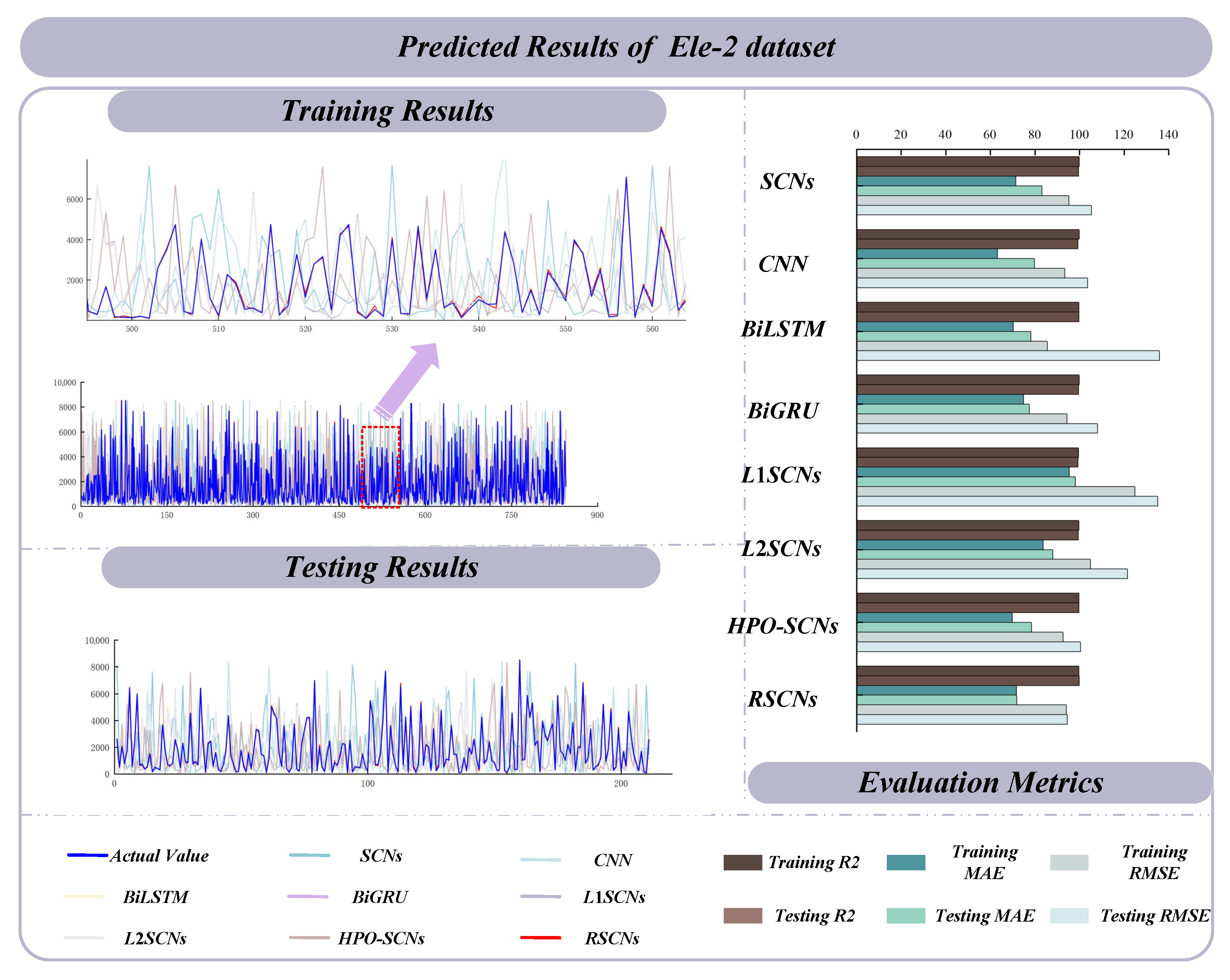
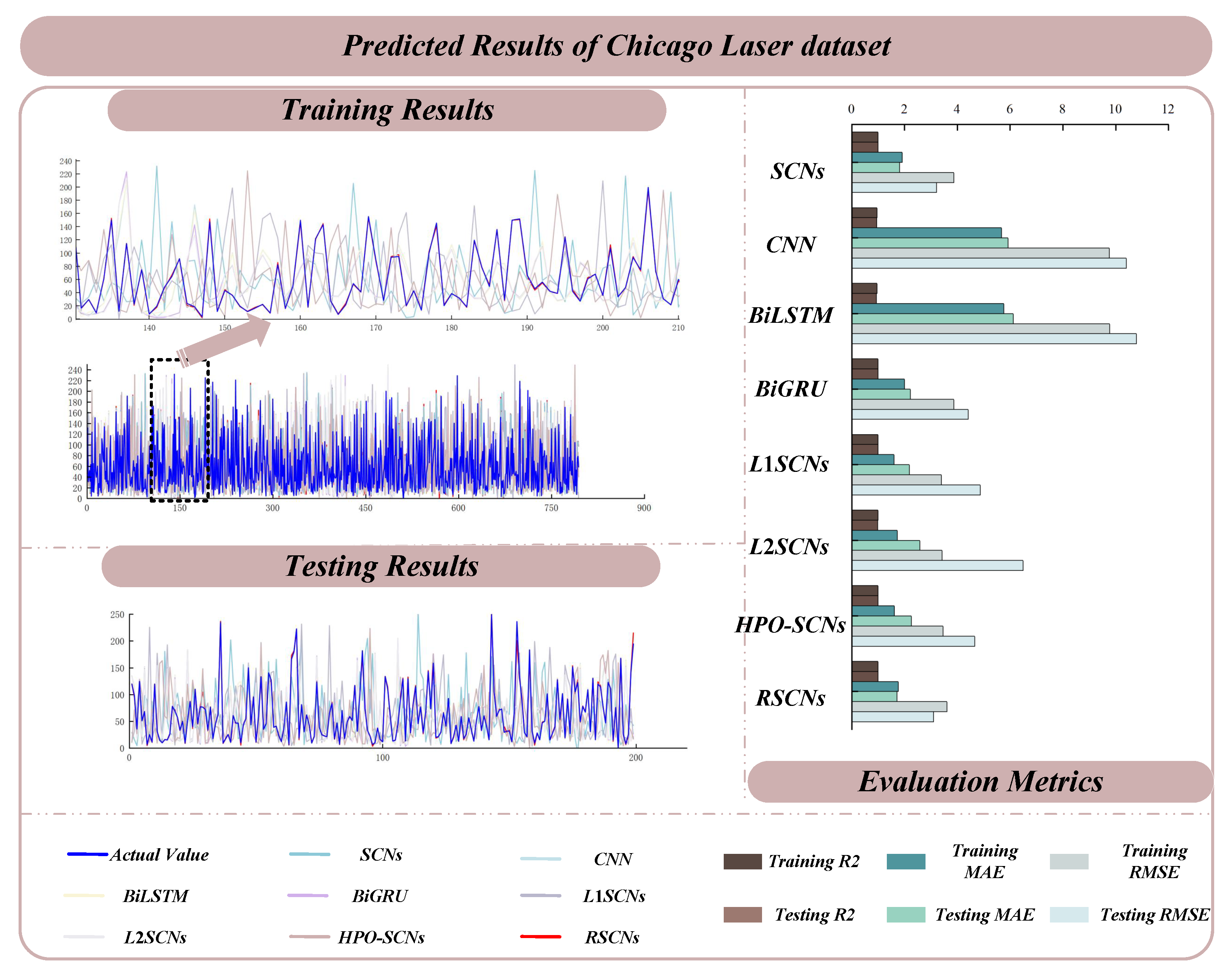
According to the description of each data set in Table 1, the Laser and Ele-2 datasets have the same number of features and a similar number of samples, but their sample values differ obviously. Figure 3 and Figure 4 illustrated the specific performance of these two datasets. Firstly, it was intuitively evident that RSCNs exhibited advantages in R 2 performance on the Laser dataset (to make the comparison more intuitive, the R 2 values in the figure were magnified 100 times). Meanwhile, the MAE and RMSE performances of the two datasets were highly similar, indicating that RSCNs did not overfit on either dataset and successfully captured the underlying patterns while avoiding overfitting risks. Observing other models, particularly HPO-SCNs with swarm intelligence optimization algorithms, revealed a certain degree of overfitting on both datasets. This suggested that although swarm intelligence optimization algorithms can obtain good parameters with powerful solving abilities, excessive pursuit of lower model residuals without corresponding regularization measures increases the risk of overfitting. Conversely, for L1SCNs and L2SCNs that explicitly incorporated regularization techniques, using default regularization strengths led to counterproductive effects when handling simple datasets. Specifically, the inclusion of regularization negatively impacted what could otherwise be satisfactory results. As shown in Table 3, both models demonstrated the worst performance across all metrics, indicating that dynamically adjusting regularization intensity according to model characteristics was crucial for achieving ideal outcomes. Meanwhile, among the compared models—CNN, BiLSTM, and BiGRU—only BiGRU demonstrated stable performance on simple datasets. In contrast, CNN and BiLSTM exhibited instability. For instance, on the Laser dataset, the R 2 scores of CNN and BiLSTM were lower than those of other models. This discrepancy may arise from two factors: first, the relatively small dataset size limited the effectiveness of training for these models; second, the complexity of parameter tuning might hinder optimal configuration. On the Ele-2 dataset, despite having a low MAE, BiLSTM exhibited a high RMSE, suggesting significant error fluctuations during multiple prediction processes.
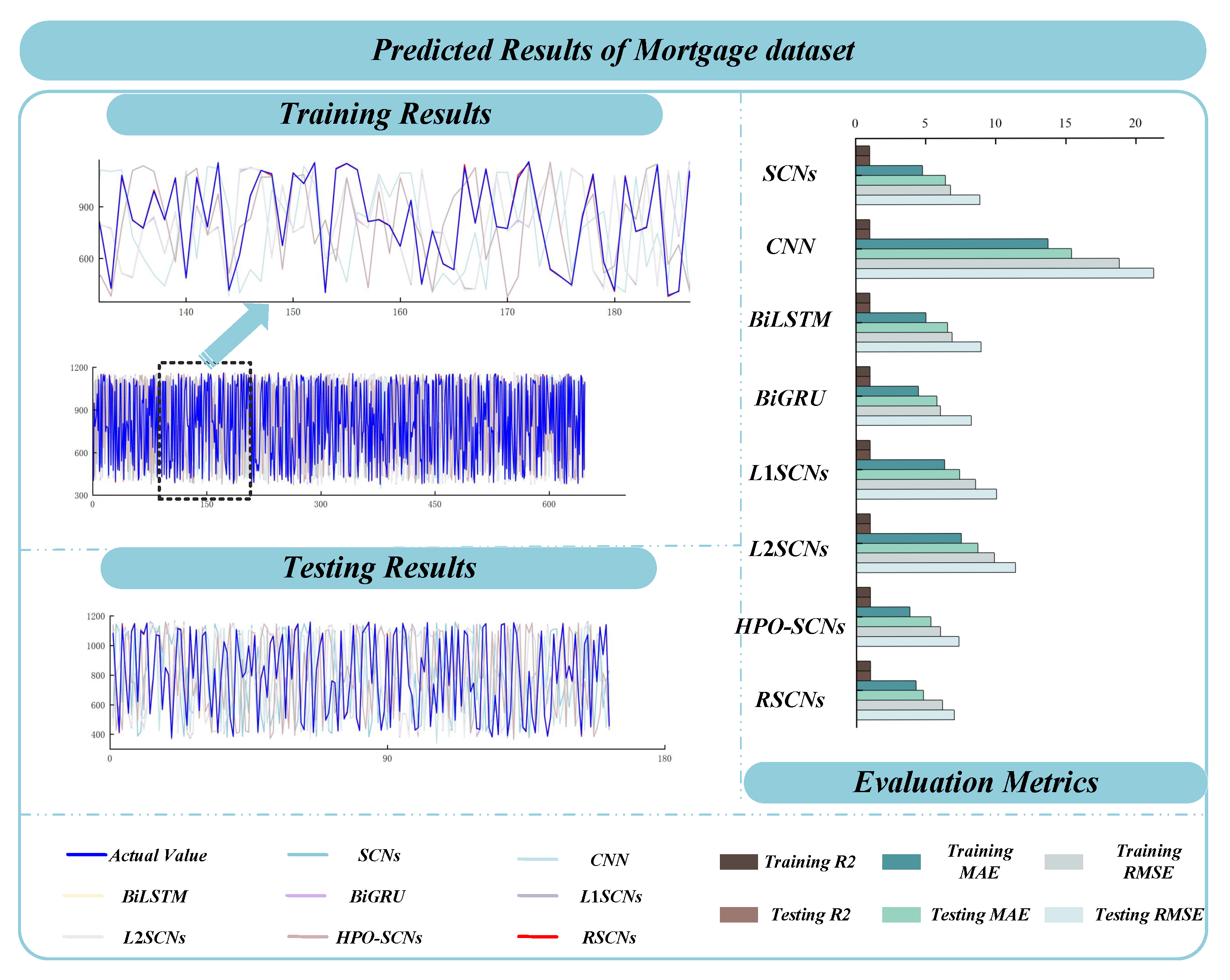
For high-dimensional Mortgage dataset with up to 15 features, as shown in Figure 5, a performance gap was observed between the prediction accuracy of SCNs and HPO-SCNs on the test set compared to RSCNs. Further analysis of the performance gap between the training and test sets for each model revealed that the differences in R 2 , MAE, and RMSE for RSCNs were only 0.015%, 10.9%, and 12.1%, respectively. In contrast, SCNs and HPO-SCNs exhibited gaps of 0.039%, 25.7%, 23.7% and 0.028%, 28.4%, 18.1%, respectively. Firstly, the gaps between the training and test sets for SCNs and HPO-SCNs were approximately double or even higher than those for RSCNs. Additionally, RSCNs achieved the best performance across all evaluation metrics, indicating their ability to balance learning capacity with adaptive regularization techniques and effectively regulate the combination of weights and biases during construction. Further examination revealed that HPO-SCNs achieved a relatively high R 2 due to their good learning capacity but exhibited higher MAE values compared to basic SCNs, suggesting that both models suffered from large absolute errors on the test set. While HPO-SCNs showed clear advantages in MAE on the training set, they exhibited overfitting, whereas SCNs, which lacked improvement mechanisms, demonstrated the largest RMSE gap of 23.7%, primarily due to high relative errors on the test set. This indicates that basic SCNs without methods to regulate learning capacity are unsuitable for high-dimensional datasets. Meanwhile, the performance of L1SCNs and L2SCNs was not particularly satisfactory. The fixed regularization strength constrained SCN performance, preventing them from achieving the desired prediction accuracy or even matching the accuracy of the original SCNs. This suggests that inappropriate regularization strength—particularly when too weak—can negatively impact prediction accuracy when handling high-dimensional complex datasets. Regarding the other three models under comparison, CNN failed to achieve competitive performance. In contrast, BiLSTM and BiGRU demonstrated performance comparable to that of SCNs.
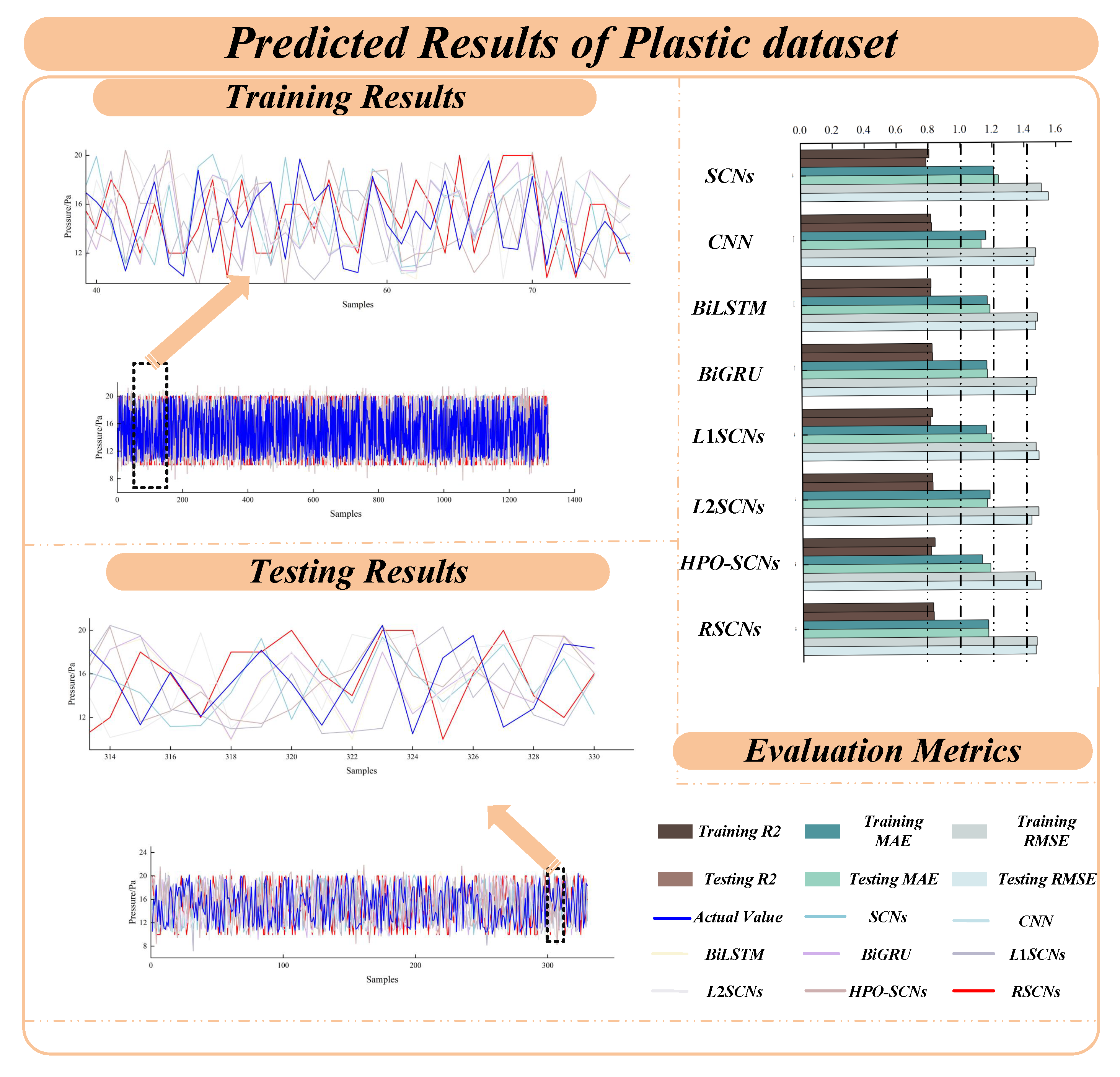
However, for the low-dimensional Plastic dataset, as shown in Figure 6, which generally exhibits small data values, fewer features, and higher oscillations, the gap between the training and test sets of SCNs and HPO-SCNs increased. Specifically, the differences in R 2 , MAE, and RMSE between the training and test sets of RSCNs were only 0.384%, 0.029%, and 0.488%, respectively, while those of SCNs and HPO-SCNs reached 2.47%, 2.65%, 2.73% and 2.91%, 4.28%, 2.52%, respectively. This indicates that RSCNs achieved outstanding performance on simple regression tasks, surpassing other models across all evaluation metrics. Notably, the gap between the training and test sets for RSCNs was only one-tenth to one-hundredth of that observed in other models, further demonstrating that its adaptive regularization technique effectively improved prediction stability. In particular, HPO-SCNs, optimized using a swarm intelligence algorithm with residuals treated as the fitness function, retained only parameter configurations that minimized residuals most efficiently. However, this approach neglected global learning capacity allocation, leading to larger generalization gaps compared to RSCNs. Based on the results, the metrics of each comparison model are no longer as favorable as those observed in previous datasets, likely due to the high volatility inherent in these datasets. At this point, the regularization techniques employed by L1SCNs and L2SCNs prove useful. It is evident that the performance of these two models on this dataset is nearly comparable to that of other models, particularly for L1SCNs, which emphasize sparsity. With appropriate adjustment of their regularization intensity, it is reasonable to predict that L1SCNs could achieve satisfactory performance on highly volatile datasets. This further highlights the necessity of dynamically adjusting regularization intensity during the model construction process. Although CNN, BiLSTM, and BiGRU demonstrated better performance compared to SCNs on the Plastic dataset, they still exhibit noticeable gaps in terms of stability and accuracy when compared with RSCNs.
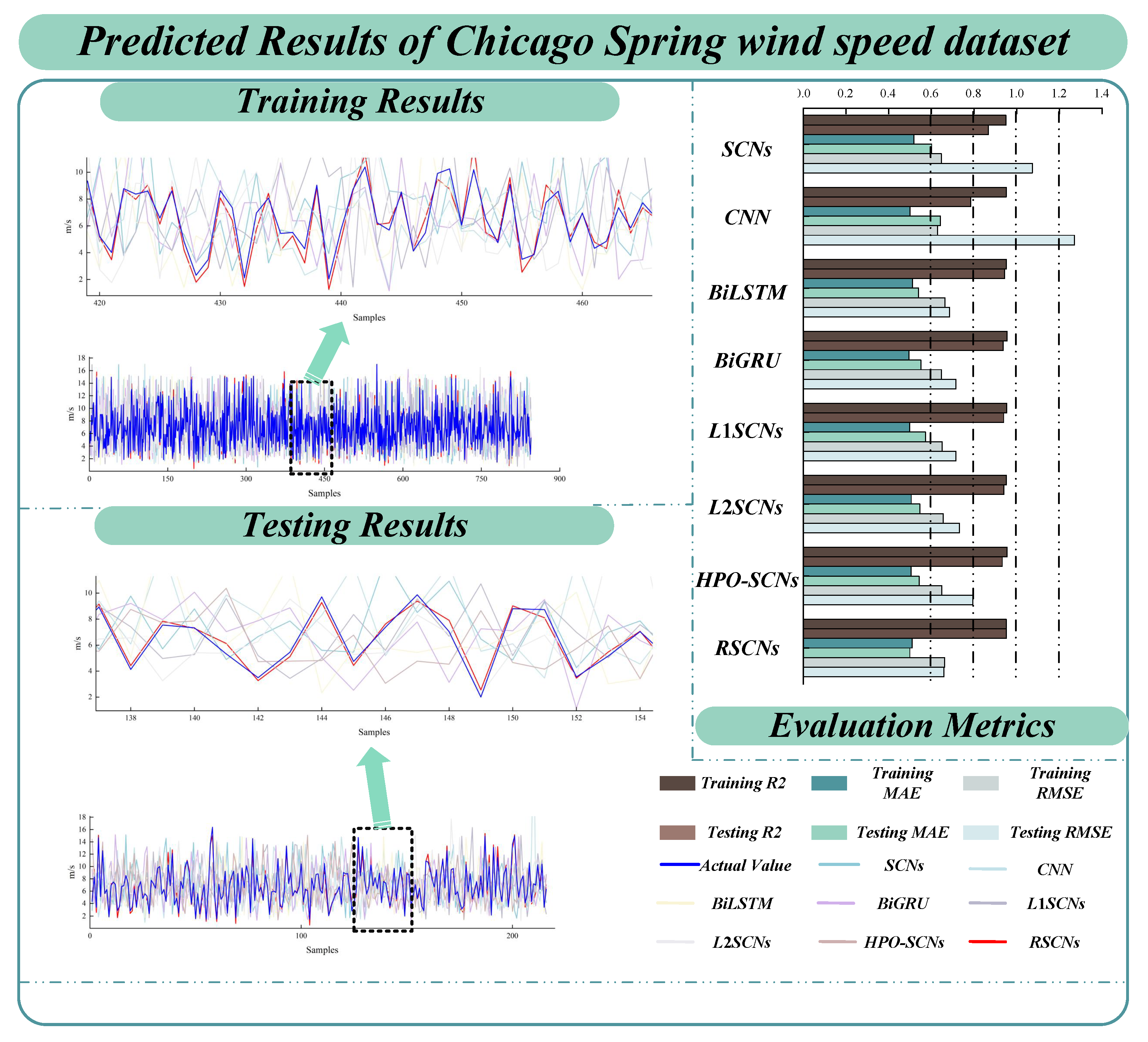
According to the performance of each model in predicting Chicago spring wind speed, as shown in Figure 7, firstly, the green curve representing SCNs deviated more from actual values than the curves of other models in both the training and test sets. Further analysis of the local zoom maps revealed that for the training set, although RSCNs were closer to actual values in most cases, HPO-SCNs reduced outliers due to their high training efficiency and exhibited comparable overall trends. For the test set, HPO-SCNs overfitted the training data, leading to deviations in the test set. While the overall trend remained within an acceptable range, the red curve representing RSCNs maintained a smaller distance from actual values, indicating that RSCNs, by incorporating regularization techniques into the model construction process, achieved better stability than HPO-SCNs. Although HPO-SCNs improved model performance, their training efficiency was compromised, and the regularization mechanism in RSCNs better regulated weight and bias generation, thereby avoiding overfitting caused by uncontrolled learning capacity while maintaining sufficient learning ability. Secondly, evaluation metrics further highlighted the differences. Although RSCNs did not exhibit a clear advantage in R 2 , their training-test set gaps were minimal (0.118%, 2.15%, and 0.419% for R 2 , MAE, and RMSE, respectively), showing distinct superiority in MAE and RMSE compared to other models. In contrast, HPO-SCNs and SCNs had much larger gaps (2.33%, 7.07%, 18.35% and 8.71%, 13.71%, 39.74%, respectively). The 39.75% RMSE gap in SCNs indicated severe overfitting, as the model performed poorly on the test set despite good training performance. While HPO-SCNs showed better performance than SCNs, their results were less stable compared to RSCNs. In fact, the wind speed dataset, characterized by both volatility and regularity, serves as an ideal benchmark for objectively comparing prediction accuracy and robustness across different models. Based on the training set metrics, the training performances of all models were largely consistent, suggesting that the learning capabilities of the compared models were comparable. However, in terms of the test set results, CNN exhibited a pronounced overfitting phenomenon, and its R 2 showed a gap of at least approximately 12% compared to other models. While BiLSTM and BiGRU maintained relatively good performance, they still demonstrated slightly less stability in prediction outcomes compared to RSCNs. From the results of SCNs, L1SCNs, and L2SCNs, it was evident that incorporating regularization techniques was essential for wind speed prediction. Regardless of whether L1 or L2 regularization was applied, the improvement in SCNs’ performance was effective.
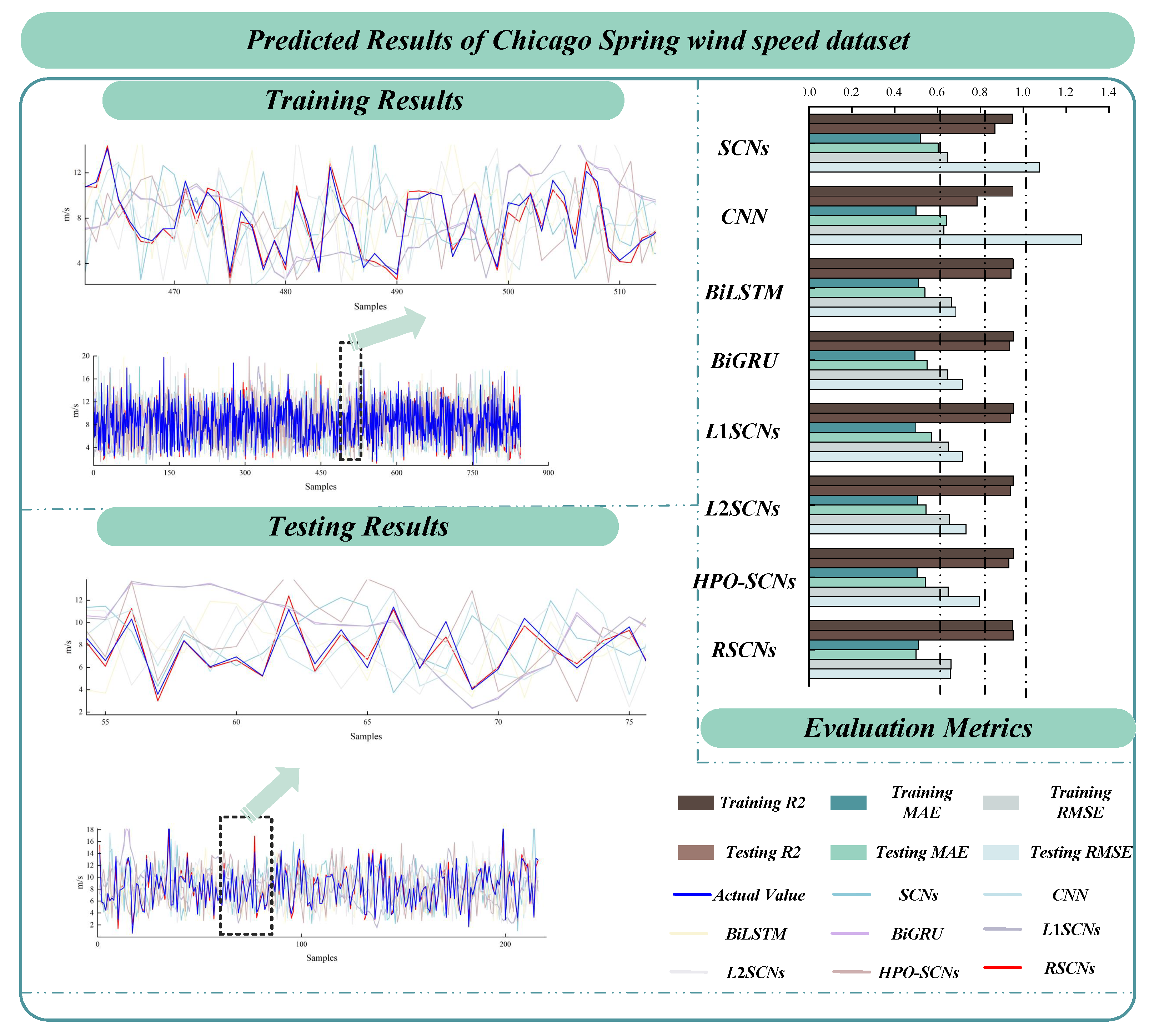
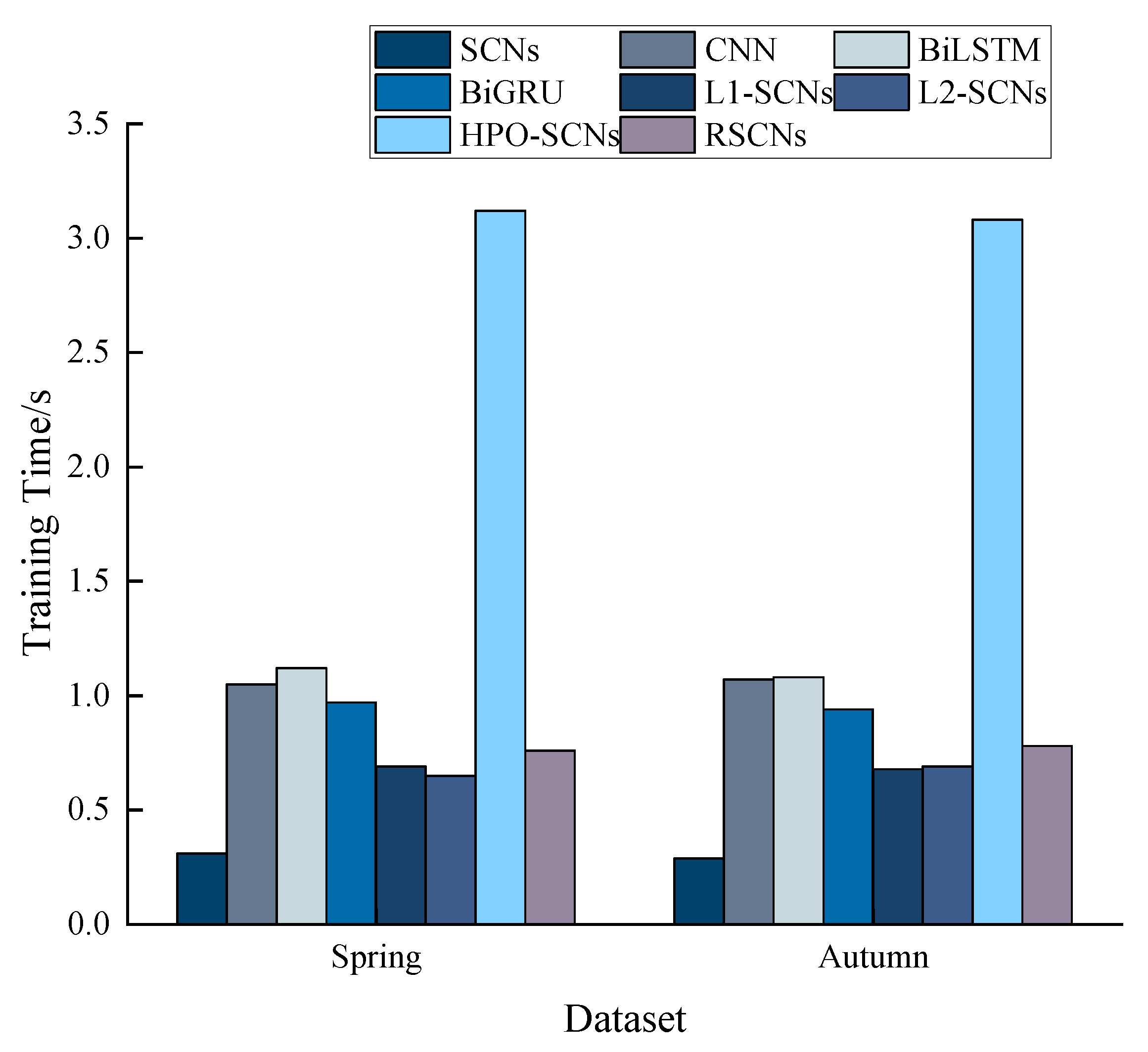
As shown in Figure 8, the performance of Chicago autumn wind speed prediction was more stable than that in spring. The prediction results for both the training and test sets exhibited reduced volatility, fewer outliers, and lower prediction difficulty compared to the spring wind speed data. While HPO-SCNs achieved better performance in the training set, their ability to process individual details remained inferior to RSCNs. Notably, only RSCNs’ average predictions closely matched the actual values at X = 150 and X = 300 in the training set. From the evaluation metrics, the gaps in R 2 , MAE, and RMSE between the training and test sets of RSCNs were minimal (0.133%, 4.88%, and 1.63%, respectively), compared to 1.12%, 7.23%, 8.07% for HPO-SCNs and 0.933%, 6.02%, 9.61% for SCNs. This demonstrates the consistent stability of RSCNs. Furthermore, the figure clearly showed that the gap between RSCNs’ training and test sets in R 2 was nearly negligible compared to SCNs and HPO-SCNs. Although the differences in MAE were small, the discrepancies in RMSE highlighted instability in the predictions of HPO-SCNs and SCNs relative to RSCNs. Among the eight models participating in the comparison, L1SCNs exhibited a notable gap in index performance relative to the other models. This suggests that even with an adapted L1 regularization technique, achieving ideal results remains challenging if parameter settings are unreasonable or there is no adaptive adjustment mechanism in place. This further underscores the critical importance of adaptively adjusting regularization intensity. However, regarding training time, as shown in Figure 9, the training times of the remaining models fall within an acceptable range, except for the notably high training time cost of HPO-SCNs.
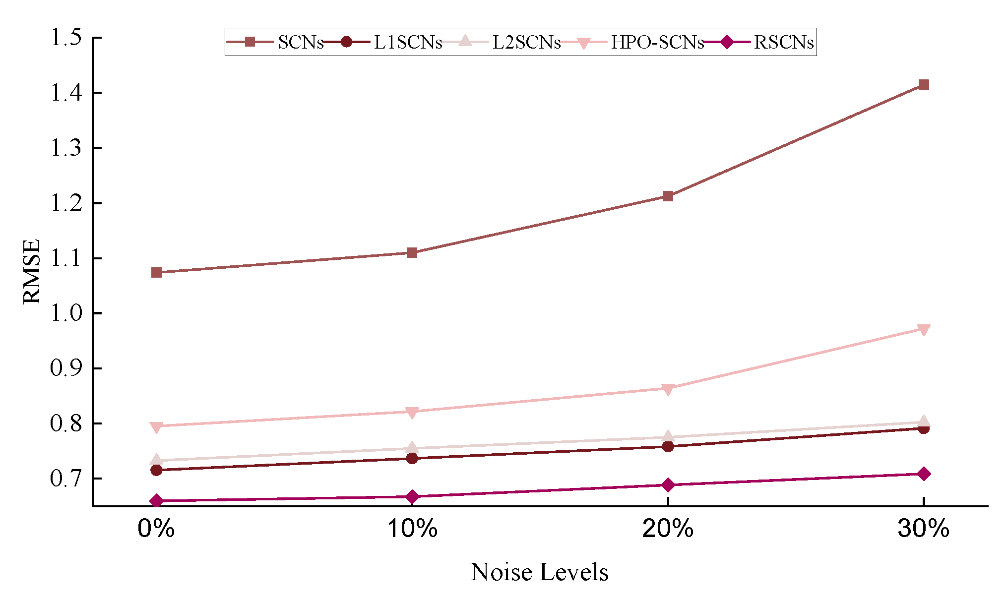
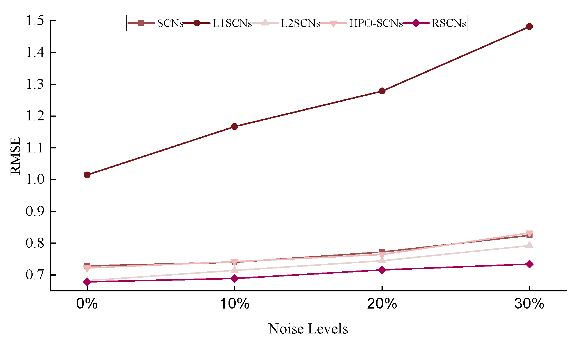
To further validate the robustness advantages of RSCNs, this study conducted supplementary comparative experiments for wind speed prediction, in which 10%, 20%, and 30% Gaussian white noise were added into two Chicago wind speed datasets to evaluate the anti-interference capabilities of all models. As illustrated in Figure 10 and Figure 11 and Table 4 and Table 5, the experimental results indicate that RSCNs consistently achieve the lowest RMSE values across multi-level noise interference tests, while demonstrating notable progressive adaptation capabilities. Specifically, the results show that regularized SCN variants (including L1SCNs, L2SCNs, and RSCNs) exhibit smoother RMSE growth trends compared to their non-regularized counterparts, effectively avoiding the abrupt RMSE increases observed in SCNs and PSO-SCNs under high-noise conditions. This confirms that the regularization mechanism enhances model stability, with RSCNs exhibiting better robustness. A quantitative analysis of the RMSE data in Table 4 and Table 5 reveals that as noise intensity increases, most models experience rising error trends, particularly at the 30% noise level, where all models show RMSE increases on the Chicago autumn wind speed dataset. Notably, despite employing regularization strategies, L1SCNs and L2SCNs still exhibit considerable error growth, whereas RSCNs’ adaptive dynamic regulation mechanism effectively mitigates error propagation, maintaining the lowest RMSE even under high-noise conditions.

5. Discussions

As evidenced by the comparative experiments, RSCNs demonstrate better predictive accuracy while maintaining consistent performance across both training and test datasets. In our opinion, this type of prediction problem does not belong to complex high-dimensional pathological datasets. In such cases, we are more concerned with the stability of prediction results, the robustness of the model, and its generalization ability. Through the above experiments, it can be observed that the MAE gap is often relatively small, while the RMSE gap is often quite significant. Particularly after Gaussian white noise injection, all competing models exhibited marked RMSE increases compared to baseline performance; this indicates that the model experiences more abnormal errors during prediction, with higher abnormal error values, which negatively impact prediction stability. Meanwhile, from an indicator perspective, the index value gaps between models are not substantial, suggesting that SCNs inherently possess better prediction performance. Regarding wind speed prediction problems, there is a notable lack of consideration for both prediction accuracy and regularization during improvements. By employing the adaptive regularization adjustment method proposed in this paper, we address the issue where fixed regularization parameters in traditional SCNs fail to adapt to different datasets, neglect parameter allocation during the overall model construction process, and cannot balance regularization strength across stages. RSCNs do not sacrifice training efficiency for better test set performance, but instead consider the overall prediction effect’s precision and stability through adaptive regularization techniques from a global perspective.

6. Conclusions

To address the regularization deficiencies of SCNs in wind speed prediction tasks, this paper proposes an improved model that integrates Elastic Net and dynamic regularization techniques, referred to as RSCNs. The main contributions and conclusions are summarized as follows:
(1)
L1 and L2 regularization are integrated through the Elastic Net and incorporated into the SCNs framework. By balancing sparsity and smoothness, this approach effectively addresses the issues of underfitting or overfitting that arise from single regularization techniques.
(2)
A dynamic loss coefficient and a penalty term based on historical error values were proposed, enabling adaptive adjustment of regularization strength and reducing the subjectivity and limitations inherent in manual hyperparameter tuning.
On the low-dimensional Plastic dataset, the RMSE gap between the training and test sets of RSCNs was only 0.465%, representing reductions of 82.8% and 81.5% compared to SCNs and HPO-SCNs, respectively, demonstrating superior stability. On high-dimensional datasets (e.g., Mortgage), RSCNs achieved a test R 2 of 0.9995, a test MAE of 4.7576, and a test RMSE of 6.792, outperforming competing models. This indicates that RSCNs can effectively capture complex nonlinear patterns while maintaining prediction stability. Wind speed prediction experiments showed that RSCNs reduced the evaluation metric gaps of SCNs on Chicago spring and autumn wind speed data by 84.65%, 99.0%, 82.8%, 98.7%, 84.4%, and 98.9%, respectively, achieving closer alignment between predicted and actual values. Through the dynamic regularization mechanism, RSCNs not only suppressed the increase in model complexity induced by higher data dimensions but also provided an efficient solution for high-dimensional prediction tasks. Furthermore, the integration of Elastic Net and the penalty term based on historical losses reduced sensitivity to hyperparameters, enabling consistent performance in practical scenarios such as sensor noise and missing data.
Despite the demonstrated effectiveness of RSCNs on both low-dimensional and high-dimensional datasets, their applicability and scalability require further validation on more complex meteorological datasets, such as multi-source or large-scale datasets. Future research should focus on extending the application of RSCNs to increasingly complex and challenging scenarios, with domain-specific enhancements to address the unique challenges posed by different data environments. Such efforts would not only broaden the application scope of RSCNs but also improve their robustness and adaptability across diverse conditions. These advancements aim to establish a solid foundation for deploying RSCNs as a versatile tool for solving real-world problems in various domains.

Author Contributions

F.J. and X.C.: Methodology, Software, Writing and Funding acquisition; Y.Y.: Methodology, Software and Writing; K.L.: Conceptualization, Methodology, Writing, Validation and Funding acquisition. All authors have read and agreed to the published version of the manuscript.

Funding

This work was supported by State Grid Liaoning Electric Power Co., Ltd. Management Technology Project (Grant no: 2024YF-25).

Data Availability Statement

This paper selected datasets from Knowledge Extraction based on Evolutionary Learning (http://www.keel.es/, (accessed on 4 June 2023)). Four benchmark regression datasets were utilized, along with wind speed data from the Chicago area during the spring and autumn of 2022 (https://www.glerl.noaa.gov/metdata/, (accessed on 20 March 2024)).

Conflicts of Interest

Authors Fuguo Jin and Xinyu Chen were employed by the company State Grid Liaoning Province Electric Power Co., Ltd. Fuxin Power Supply Company. The remaining authors declare that the research was conducted in the absence of any commercial or financial relationships that could be construed as a potential conflict of interest.

References

  1. Zhang, Z.; Lin, L.; Gao, S.; Wang, J.; Zhao, H.; Yu, H. A machine learning model for hub-height short-term wind speed prediction. Nat. Commun. 2025, 16, 3195. [Google Scholar] [CrossRef]
  2. Han, Y.; Hu, X.; Li, K. Chaotic property based multi-interval informer modeling method for long-term photovoltaic power generation prediction. Appl. Soft Comput. 2025, 184, 113843. [Google Scholar] [CrossRef]
  3. Ye, L.; Zhao, Y.; Zeng, C.; Zhang, C. Short-term wind power prediction based on spatial model. Renew. Energy 2017, 101, 1067–1074. [Google Scholar] [CrossRef]
  4. Ouyang, T.; Zha, X.; Qin, L. A combined multivariate model for wind power prediction. Energy Convers. Manag. 2017, 144, 361–373. [Google Scholar] [CrossRef]
  5. Miao, S.; Yang, H.; Gu, Y. A wind vector simulation model and its application to adequacy assessment. Energy 2018, 148, 324–340. [Google Scholar] [CrossRef]
  6. Chen, G.; Wang, G. A supervised learning algorithm for spiking neurons using spike train kernel based on a unit of pair-spike. IEEE Access 2020, 8, 53427–53442. [Google Scholar] [CrossRef]
  7. Chen, G.; Wang, G. Tstkd: Triple-spike train kernel-driven supervised learning algorithm. Pattern Recognit. 2025, 164, 111525. [Google Scholar] [CrossRef]
  8. Wang, D.; Li, M. Stochastic configuration networks: Fundamentals and algorithms. IEEE Trans. Cybern. 2017, 47, 3466–3479. [Google Scholar] [CrossRef]
  9. Li, J.; Wang, D. 2D convolutional stochastic configuration networks. Knowl.-Based Syst. 2024, 300, 112249. [Google Scholar] [CrossRef]
  10. Zhou, T.; Wang, Y.; Yang, G.; Zhang, C.; Wang, J. Greedy stochastic configuration networks for ill-posed problems. Knowl.-Based Syst. 2023, 269, 110464. [Google Scholar] [CrossRef]
  11. Zhang, C.; Wang, Y.; Zhang, D. Greedy deep stochastic configuration networks ensemble with boosting negative correlation learning. Inf. Sci. 2024, 680, 121140. [Google Scholar] [CrossRef]
  12. Dang, G.; Wang, D. Self-organizing recurrent stochastic configuration networks for nonstationary data modeling. IEEE Trans. Ind. Inform. 2025, 21, 4820–4829. [Google Scholar] [CrossRef]
  13. Wang, D.; Dang, G. Fuzzy recurrent stochastic configuration networks for industrial data analytics. IEEE Trans. Fuzzy Syst. 2025, 33, 1178–1191. [Google Scholar] [CrossRef]
  14. Sun, K.; Yang, C.; Gao, C.; Wu, X.; Zhao, J. Development of an online updating stochastic configuration network for the soft-sensing of the semi-autogenous ball mill crusher system. IEEE Trans. Instrum. Meas. 2024, 73, 1–11. [Google Scholar] [CrossRef]
  15. Han, Y.; Yu, Y.; Wu, H.; Li, K. Multi-level optimizing of parameters in stochastic configuration networks based on cloud model and nutcracker optimization algorithm. Inf. Sci. 2025, 689, 121495. [Google Scholar] [CrossRef]
  16. Li, M.; Huang, C.; Wang, D. Robust stochastic configuration networks with maximum correntropy criterion for uncertain data regression. Inf. Sci. 2019, 473, 73–86. [Google Scholar] [CrossRef]
  17. Lu, J.; Ding, J. Mixed-distribution-based robust stochastic configuration networks for prediction interval construction. IEEE Trans. Ind. Inform. 2019, 16, 5099–5109. [Google Scholar] [CrossRef]
  18. Wu, H.; Zhang, A.; Han, Y.; Nan, J.; Li, K. Fast stochastic configuration network based on an improved sparrow search algorithm for fire flame recognition. Knowl.-Based Syst. 2022, 245, 108626. [Google Scholar] [CrossRef]
  19. Han, Y.; Yu, Y.; Li, K. Adaptive inertia weights: An effective way to improve parameter estimation of hidden layer in stochastic configuration networks. Int. J. Mach. Learn. Cybern. 2025, 16, 2203–2218. [Google Scholar] [CrossRef]
  20. Dai, W.; Ning, C.; Nan, J.; Wang, D. Stochastic configuration networks for imbalanced data classification. Int. J. Mach. Learn. Cybern. 2022, 13, 2843–2855. [Google Scholar] [CrossRef]
  21. Zhao, L.; Zou, S.; Guo, S.; Huang, M. Ball mill load condition recognition model based on regularized stochastic configuration networks. Control Eng. China 2020, 27, 1–7. [Google Scholar]
  22. Pan, C.; Xv, J.; Weng, Y. A fault identification method of chemical process based on manifold regularized stochastic configuration network. Chin. J. Sci. Instrum. 2021, 42, 219–226. [Google Scholar]
  23. Szabo, Z.; Lorincz, A. L1 regularization is better than l2 for learning and predicting chaotic systems. arXiv 2004, arXiv:cs/0410015. [Google Scholar] [CrossRef]
  24. Zou, H. The adaptive lasso and its oracle properties. J. Am. Stat. Assoc. 2006, 101, 1418–1429. [Google Scholar] [CrossRef]
  25. Zhao, P.; Yu, B. Stagewise lasso. J. Mach. Learn. Res. 2007, 8, 2701–2726. [Google Scholar]
  26. Zhang, Z.; Xu, Y.; Yang, J.; Li, X.; Zhang, D. A survey of sparse representation: Algorithms and applications. IEEE Access 2017, 3, 490–530. [Google Scholar] [CrossRef]
  27. Zou, H.; Hastie, T. Regularization and variable selection via the elastic net. J. R. Stat. Soc. 2005, 67, 768. [Google Scholar] [CrossRef]
  28. Liu, J.; Liu, Y.; Ma, Y.; Fu, Y. Smoothing l1 regularization for stochastic configuration networks. Control Decis. 2024, 39, 813–818. [Google Scholar]
  29. Xiong, B.; Meng, X.; Xiong, G.; Ma, H.; Lou, L.; Wang, Z. Multi-branch wind power prediction based on optimized variational mode decomposition. Energy Rep. 2022, 8, 11181–11191. [Google Scholar] [CrossRef]
  30. Yu, M.; Niu, D.; Gao, T.; Wang, K.; Sun, L.; Li, M.; Xu, X. A novel framework for ultra-short-term interval wind power prediction based on rf-woa-vmd and bigru optimized by the attention mechanism. Energy 2023, 269, 126738. [Google Scholar] [CrossRef]
  31. Wang, Z.; Ying, Y.; Kou, L.; Ke, W.; Wan, J.; Yu, Z.; Liu, H.; Zhang, F. Ultra-short-term offshore wind power prediction based on pca-ssa-vmd and bilstm. Sensors 2024, 24, 444. [Google Scholar] [CrossRef] [PubMed]
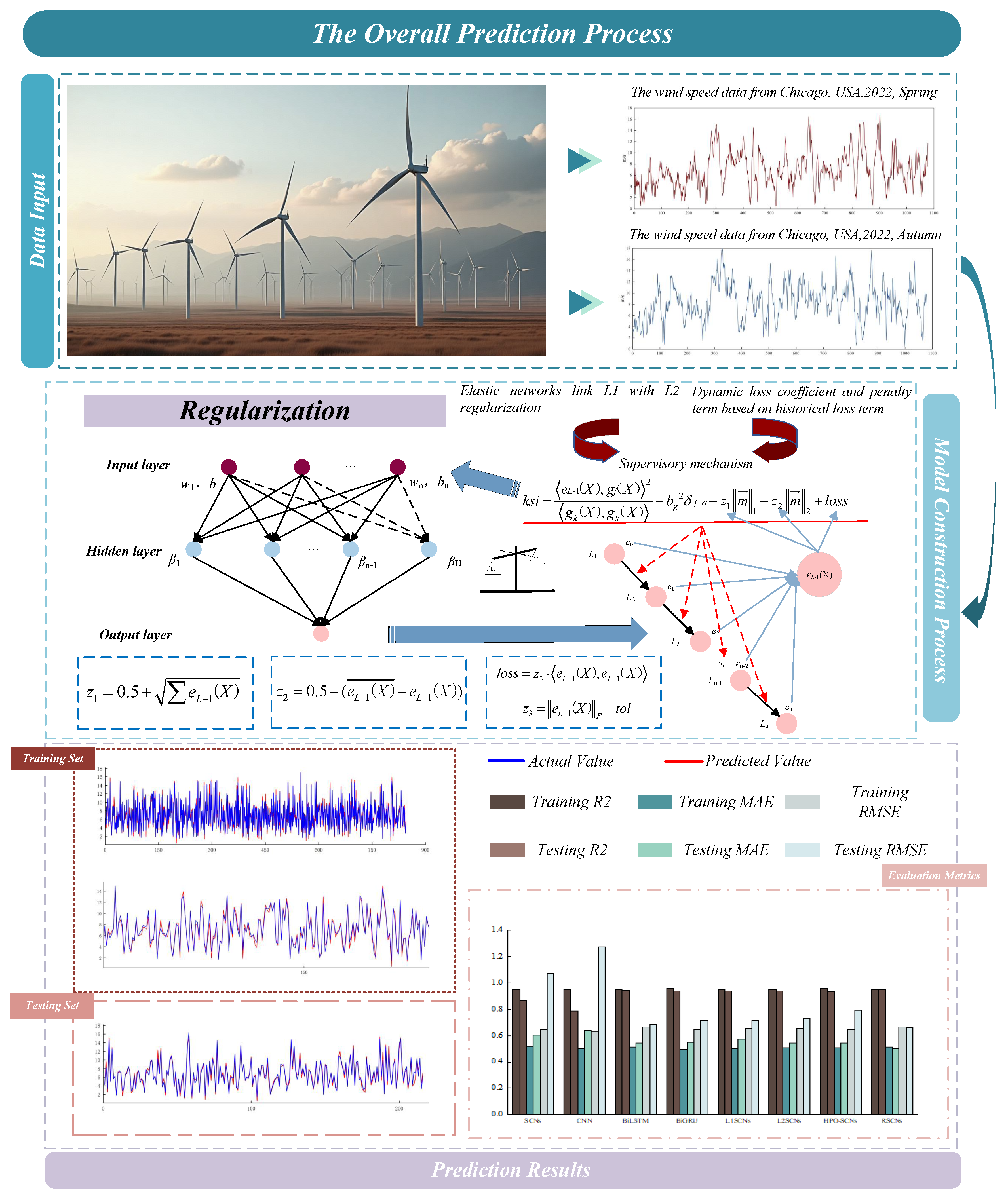
Figure 1. Flow chart of overall prediction process.
Energies 18 06170 g001
Figure 2. Original wind speed sequence.
Energies 18 06170 g002
Figure 3. Fitting curve and horizontal comparison of evaluation indicators of different algorithms on Ele-2.
Energies 18 06170 g003
Figure 4. Fitting curve and horizontal comparison of evaluation indicators of different algorithms on Laser.
Energies 18 06170 g004
Figure 5. Fitting curve and horizontal comparison of evaluation indicators of different algorithms on Mortgage.
Energies 18 06170 g005
Figure 6. Fitting curve and horizontal comparison of evaluation indicators of different algorithms on Plastic.
Energies 18 06170 g006
Figure 7. Fitting curve and horizontal comparison of evaluation indicators of different algorithms on Chicago Spring Wind Speed.
Energies 18 06170 g007
Figure 8. Fitting curve and horizontal comparison of evaluation indicators of different algorithms on Chicago Autumn.
Energies 18 06170 g008
Figure 9. Training time of each model on the Chicago wind speed datasets.
Energies 18 06170 g009
Figure 10. RMSE curves of different algorithms on Chicago Spring wind speed dataset with varying noise levels.
Energies 18 06170 g010
Figure 11. RMSE curves of different algorithms on Chicago Autumn wind speed dataset with varying noise levels.
Energies 18 06170 g011
Table 1. Regression dataset description.
DatasetsFeaturesInstancesBrief Introduction
Plastic21650The objective is to determine the amount of pressure a given piece of plastic can withstand when subjected to a specific pressure strength at a fixed temperature. Input: Strength and Temperature; Output: Pressure.
Ele-241056Electrical maintenance data consist of four input variables. Input: Reactive power at 110 kV side, 35 kV side, 10 kV side and Reactive power output of reactive power compensation device; Output: Reactive power on the high voltage side of the main transformer.
Laser4993The dataset originates from the Santa Fe Time Series Competition database and comprises four features with 993 entries. Initially, this dataset was a univariate time series recording the chaotic state of a far-infrared laser. By selecting four consecutive values as input, the output is to predict the subsequent value.
Mortgage151049This file contains weekly Economic data for the USA from 4 January 1980, to 4 February 2000. Based on the provided features, the objective is to predict the 30-Year Conventional Mortgage Rate. Input: 16 kinds of variables such as MonthCDRate, DemandDeposits, FederalFunds, etc. Output: 30Y-CMortgageRate.
Table 2. Model parameter setting.
ModelParameter Settings
BiGRU L e a r n R a t e D r o p P e r i o d = 400; M a x E p o c h s = 500; L e a r n i n g r a t e = 0.01.
BiLSTM M i n i B a t c h S i z e = 128; M a x E p o c h s = 1500; L e a r n i n g r a t e = 0.001.
L1SCNs, L2SCNs α = 0.5
Table 3. Comparison of prediction results of several models under different datasets.
DatasetAlgorithmTrainingTesting
R 2 MAE RMSE R 2 MAE RMSE
Ele-2SCNs0.9976 ± 0.001071.4170 ± 7.230495.2537 ± 9.66310.9951 ± 0.001086.7361 ± 7.9880107.8005 ± 10.7783
CNN0.9980 ± 0.001063.1699 ± 6.030792.3980 ± 9.92670.9926 ± 0.001191.1139 ± 8.8537144.4438 ± 15.1040
BiLSTM0.9975 ± 0.001470.2551 ± 7.004095.2117 ± 8.60730.9965 ± 0.001081.2314 ± 7.3015137.3628 ± 14.3399
BiGRU0.9976 ± 0.001074.9013 ± 7.040794.3403 ± 9.15570.9934 ± 0.000987.4428 ± 7.9001141.5133 ± 13.8105
L1SCNs0.9957 ± 0.001195.3727 ± 10.2334124.8383 ± 13.71310.9908 ± 0.0010102.1128 ± 11.0060155.6993 ± 15.6332
L2SCNs0.9970 ± 0.001083.7090 ± 8.2304104.9157 ± 11.00470.9928 ± 0.001088.0278 ± 8.8123122.3325 ± 12.6332
HPO-SCNs0.9975 ± 0.001169.7793 ± 6.100492.5619 ± 9.11160.9966 ± 0.001079.1055 ± 7.3981102.4117 ± 10.4069
RSCNs0.9974 ± 0.001171.6095 ± 6.542394.1306 ± 9.32830.9971 ± 0.001075.2506 ± 6.266799.5576 ± 9.5196
LaserSCNs0.9934 ± 0.00111.9084 ± 0.29933.8698 ± 1.21310.9921 ± 0.00091.9997 ± 0.35563.8830 ± 1.2139
CNN0.9588 ± 0.00125.6749 ± 1.03159.7562 ± 1.92670.9325 ± 0.00117.1779 ± 1.931213.7063 ± 2.4499
BiLSTM0.9586 ± 0.00115.7630 ± 1.01419.7795 ± 1.61790.9335 ± 0.00136.3766 ± 1.277311.5503 ± 2.0863
BiGRU0.9935 ± 0.00101.9917 ± 0.27133.8639 ± 0.49270.9860 ± 0.00092.2394 ± 0.37704.8089 ± 0.9031
L1SCNs0.9946 ± 0.00111.6940 ± 0.23703.3936 ± 0.71670.9892 ± 0.00102.1979 ± 0.27384.8680 ± 0.6117
L2SCNs0.9949 ± 0.00101.7218 ± 0.19833.4257 ± 0.86310.9664 ± 0.00102.6843 ± 0.97076.1735 ± 1.0033
HPO-SCNs0.9943 ± 0.00121.6066 ± 0.21213.4615 ± 1.19630.9905 ± 0.00272.1503 ± 0.40634.6004 ± 1.2102
RSCNs0.9909 ± 0.00121.7568 ± 0.24633.6045 ± 1.20690.9930 ± 0.00102.0012 ± 0.07273.3159 ± 1.1136
MortgageSCNs0.9993 ± 0.00024.7576 ± 0.73046.7721 ± 1.81150.9980 ± 0.00057.0892 ± 1.44399.3939 ± 2.0125
CNN0.9948 ± 0.001413.7083 ± 1.838718.7895 ± 1.92130.9933 ± 0.000815.5009 ± 1.978121.8564 ± 3.1196
BiLSTM0.9993 ± 0.00085.0023 ± 1.11716.8520 ± 1.66830.9987 ± 0.00106.7349 ± 1.80139.0836 ± 2.0009
BiGRU0.9995 ± 0.00104.4419 ± 0.72176.0152 ± 1.20170.9988 ± 0.00096.7153 ± 1.44289.1326 ± 1.8097
L1SCNs0.9989 ± 0.00116.3121 ± 1.21148.5141 ± 1.91400.9971 ± 0.00109.4081 ± 1.629610.8934 ± 2.4033
L2SCNs0.9986 ± 0.00107.4919 ± 1.77279.8601 ± 2.10170.9973 ± 0.00109.2103 ± 1.911912.2874 ± 2.7737
HPO-SCNs0.9997 ± 0.00023.8093 ± 0.49616.0048 ± 1.37940.9989 ± 0.00027.2106 ± 1.40019.3117 ± 1.7090
RSCNs0.9996 ± 0.00024.2476 ± 0.77836.1398 ± 1.55370.9991 ± 0.00026.4081 ± 1.19288.91080 ± 1.3774
PlasticSCNs0.8063 ± 0.03231.2085 ± 0.10321.5096 ± 0.31140.7856 ± 0.03661.2663 ± 0.13171.6179 ± 0.3912
CNN0.8148 ± 0.02211.1577 ± 0.02171.4709 ± 0.12670.8104 ± 0.02251.1785 ± 0.07641.9578 ± 0.1436
BiLSTM0.8128 ± 0.02181.1650 ± 0.03401.4789 ± 0.04730.8116 ± 0.01211.1896 ± 0.06291.5711 ± 0.1809
BiGRU0.8167 ± 0.03151.1597 ± 0.04071.4636 ± 0.15570.8123 ± 0.01881.1805 ± 0.03911.4819 ± 0.0781
L1SCNs0.8191 ± 0.03131.1538 ± 0.03341.4543 ± 0.10310.8059 ± 0.01191.1931 ± 0.08161.5115 ± 0.1129
L2SCNs0.8136 ± 0.03101.1724 ± 0.03141.4795 ± 0.07470.8095 ± 0.01081.1631 ± 0.03041.5251 ± 0.0633
HPO-SCNs0.8284 ± 0.02911.1252 ± 0.09391.4550 ± 0.28710.8081 ± 0.02171.1794 ± 0.11431.5424 ± 0.2926
RSCNs0.8164 ± 0.02131.1598 ± 0.9811.4625 ± 0.09350.8128 ± 0.02231.1702 ± 0.11041.4632 ± 0.2628
Spring
wind
speed
SCNs0.9502 ± 0.01020.5197 ± 0.10330.6473 ± 0.13080.8665 ± 0.00770.6217 ± 0.12261.1286 ± 0.3118
CNN0.9518 ± 0.02210.4999 ± 0.04170.6142 ± 0.12670.7829 ± 0.02050.6591 ± 0.09080.8433 ± 0.0416
BiLSTM0.9524 ± 0.02080.5114 ± 0.07400.6642 ± 0.14730.9419 ± 0.01170.5618 ± 0.06110.7027 ± 0.1039
BiGRU0.9548 ± 0.02150.4956 ± 0.05770.6482 ± 0.10070.9355 ± 0.02100.5701 ± 0.04460.7281 ± 0.0591
L1SCNs0.9540 ± 0.02130.4989 ± 0.03180.7153 ± 0.09310.9381 ± 0.01310.5839 ± 0.06990.7303 ± 0.1109
L2SCNs0.9527 ± 0.02100.5064 ± 0.02980.6554 ± 0.06780.9415 ± 0.01060.5437 ± 0.03880.7285 ± 0.0326
HPO-SCNs0.9550 ± 0.001930.5047 ± 0.09030.6496 ± 0.12560.9319 ± 0.00920.5387 ± 0.12320.7710 ± 0.1988
RSCNs0.9514 ± 0.001630.5107 ± 0.10020.6624 ± 0.11180.9421 ± 0.00490.5169 ± 0.07720.6813 ± 0.1122
Autumn
wind
speed
SCNs0.9570 ± 0.00850.5174 ± 0.12660.6586 ± 0.17580.9479 ± 0.00720.5637 ± 0.13360.7446 ± 0.2305
CNN0.9587 ± 0.02110.5053 ± 0.04460.6535 ± 0.12670.9359 ± 0.02290.6425 ± 0.09050.7883 ± 0.1671
BiLSTM0.9578 ± 0.01180.5085 ± 0.05700.6570 ± 0.10730.9477 ± 0.01050.5726 ± 0.05530.7209 ± 0.1115
BiGRU0.9587 ± 0.02050.5061 ± 0.03770.6540 ± 0.10070.9385 ± 0.02030.5818 ± 0.03170.7241 ± 0.0646
L1SCNs0.9589 ± 0.02430.5115 ± 0.03180.6521 ± 0.05310.8913 ± 0.01710.6959 ± 0.05180.9447 ± 0.1696
L2SCNs0.9564 ± 0.02120.5229 ± 0.02880.6712 ± 0.05780.9517 ± 0.02080.5361 ± 0.03180.7123 ± 0.0651
HPO-SCNs0.9594 ± 0.00760.5052 ± 0.12890.6605 ± 0.17930.9433 ± 0.00630.5680 ± 0.12620.7414 ± 0.1951
RSCNs0.9560 ± 0.00410.5613 ± 0.11990.6672 ± 0.16480.9543 ± 0.00530.5221 ± 0.11030.6921 ± 0.1538
Note: Bold is the best.
Table 4. Prediction results of different algorithms on Chicago Spring wind speed dataset with different noise levels.
AlgorithmsNoise Levels
0% 10% 20% 30%
SCNs 1.0739 ± 0.3481 1.1101 ± 0.4145 1.2124 ± 0.4170 1.4146 ± 0.0162
CNN 0.8293 ± 0.0476 0.9026 ± 0.0467 0.9522 ± 0.0473 1.1121 ± 0.0577
BiLSTM 0.6853 ± 0.1042 0.7124 ± 0.1165 0.7528 ± 0.1168 0.8129 ± 0.1177
BiGRU 0.7160 ± 0.0631 0.7425 ± 0.0659 0.7726 ± 0.0676 0.8126 ± 0.0765
L1SCNs 0.7153 ± 0.1011 0.7367 ± 0.1142 0.7582 ± 0.1155 0.7912 ± 0.1126
L2SCNs 0.7326 ± 0.0623 0.7547 ± 0.0638 0.7750 ± 0.0644 0.8025 ± 0.0659
HPO-SCNs 0.7955 ± 0.2037 0.8218 ± 0.2139 0.8643 ± 0.2149 0.9722 ± 0.2162
RSCNs0.6597 ± 0.10910.6674 ± 0.10990.6885 ± 0.10820.7086 ± 0.1426
Note: Bold is the best.
Table 5. Prediction results of different algorithms on Chicago Autumn wind speed dataset with different noise levels.
AlgorithmsNoise Levels
0% 10% 20% 30%
SCNs 0.7284 ± 0.2132 0.7401 ± 0.2145 0.7724 ± 0.0170 0.8246 ± 0.0162
CNN 0.7679 ± 0.1476 0.7826 ± 0.01537 0.8122 ± 0.1573 0.8521 ± 0.1777
BiLSTM 0.7082 ± 0.1007 0.7324 ± 0.1065 0.7528 ± 0.1168 0.8019 ± 0.1177
BiGRU 0.7564 ± 0.0691 0.7725 ± 0.0699 0.8126 ± 0.0676 0.8626 ± 0.0865
L1SCNs 1.0146 ± 0.1548 1.1667 ± 0.1542 1.2782 ± 0.1655 1.4812 ± 0.2126
L2SCNs 0.6823 ± 0.0663 0.7147 ± 0.0668 0.7450 ± 0.0744 0.7925 ± 0.0859
HPO-SCNs 0.7223 ± 0.1943 0.7418 ± 0.1939 0.7643 ± 0.1969 0.8322 ± 0.2262
RSCNs0.6782 ± 0.15910.6891 ± 0.14830.7158 ± 0.14680.7341 ± 0.1796
Note: Bold is the best.
Disclaimer/Publisher’s Note: The statements, opinions and data contained in all publications are solely those of the individual author(s) and contributor(s) and not of MDPI and/or the editor(s). MDPI and/or the editor(s) disclaim responsibility for any injury to people or property resulting from any ideas, methods, instructions or products referred to in the content.