Short-Term Wind Power Forecasting with Transformer-Based Models Enhanced by Time2Vec and Efficient Attention

Abstract

Accurate wind power forecasting is essential to optimize wind farm operations and ensure the stable integration of renewable energy into the grid. This study explores Transformer-based architectures to address the challenges of wind variability and temporal dependencies in short-term forecasting. A sensitivity analysis on model architecture is conducted, incorporating Time2Vec—a temporal encoding technique that captures complex temporal patterns. In addition, we replace the standard FullAttention mechanism with ProbSparse Attention, FlowAttention and FlashAttention, resulting in the Informer, Flowformer and Flashformer models, to improve computational efficiency while maintaining predictive accuracy. The novelty of this work lies in applying FlashAttention within the context of wind power forecasting and integrating Time2Vec into the Informer, Flowformer and Flashformer models. We propose four architectures—T2V-Transformer, T2V-Informer, T2V-Flowformer, and T2V-Flashformer—and compare them against benchmark models: Multi-Layer Perceptron (MLP), Long Short-Term Memory (LSTM), and DLinear. Real-world data from a wind farm in the Northeast of Brazil is used under two forecasting scenarios. In Scenario A, T2V-Transformer, T2V-Informer and T2V-Flashformer achieved Improvement over Reference RMSE (IoR-RMSE) scores of 17.73%, 17.59% and 16.67%, respectively. In Scenario B, T2V-Flowformer and T2V-Flashformer reached 27.84% and 27.45%, respectively. These results confirm the effectiveness of the proposed models in advancing short-term wind power forecasting.

1. Introduction

Over the last few decades, the world has faced problems related to environmental impacts. This is a direct consequence of rapid economic development and large-scale population growth [1]. As a result, the search for renewable energy sources has become increasingly necessary. Therefore, wind energy stands out as a renewable source type that has lower environmental impacts compared to non-renewable sources [2]. According to Ref. [3], 2023 was a record year for renewable energy, with new installations of 510 GW (all renewables) and 117 GW (wind)—an increase of almost 50% compared to the previous year for both cases. This growth is expected to reach 3 TW of cumulative wind energy capacity by 2030. This form of renewable energy serves as a fundamental solution to meet the high demands for electrical energy and mitigate the environmental impacts on the planet. Consequently, with the increasing share of wind energy in the global energy matrix, maximizing the productive efficiency of wind farms is fundamental.

However, wind energy faces operating and maintenance planning challenges due to the stochastic nature and non-linearity of wind speeds. This may compromise the productivity and reliability of wind farms [4]. It may also overload turbines and reduce the Remaining Useful Life (RUL) of critical components [5] To maximize production efficiency and support effective planning in wind farm management, accurate forecasts of wind energy supply and availability are extremely important.

Wind power forecasting is essential for ensuring grid stability and optimizing the integration of renewable energy sources. An accurate forecasting process relies on a clear understanding of time series concepts. A time series is a sequence of observations collected over time, where each value is associated with a specific instant or period. Historical time series data serve as inputs (or regressors) in modeling, with a time step—often a multiple of ∇_t—defining the interval between consecutive inputs. While the time step is an inherent characteristic of the series, the time interval is a key component of the forecasting strategy. Another crucial parameter is the forecast horizon, which specifies the future time span (in time steps) for which predictions are made [6]. Time series generally have three main components: trend, seasonality, and noise [7]. Trends represent underlying long-term patterns, such as gradual growth or steady decline over time. Seasonality refers to cyclical and repetitive patterns that occur at regular and predictable intervals, such as daily or annual variations. Noise, on the other hand, is the unpredictable part of the time series, composed of random fluctuations that do not follow any clear pattern and may be caused by unexpected external factors or measurement errors. To capture specific patterns related to these components, techniques such as the Fast Fourier Transform (FFT) [8], Wavelet Transform [9], Complete Ensemble Empirical Mode Decomposition with Adaptive Noise (CEEMDAN) [10], among others, were proposed. In wind power applications, short-term forecasts range from minutes to hours, medium-term forecasts span days to weeks, and long-term forecasts extend to months.

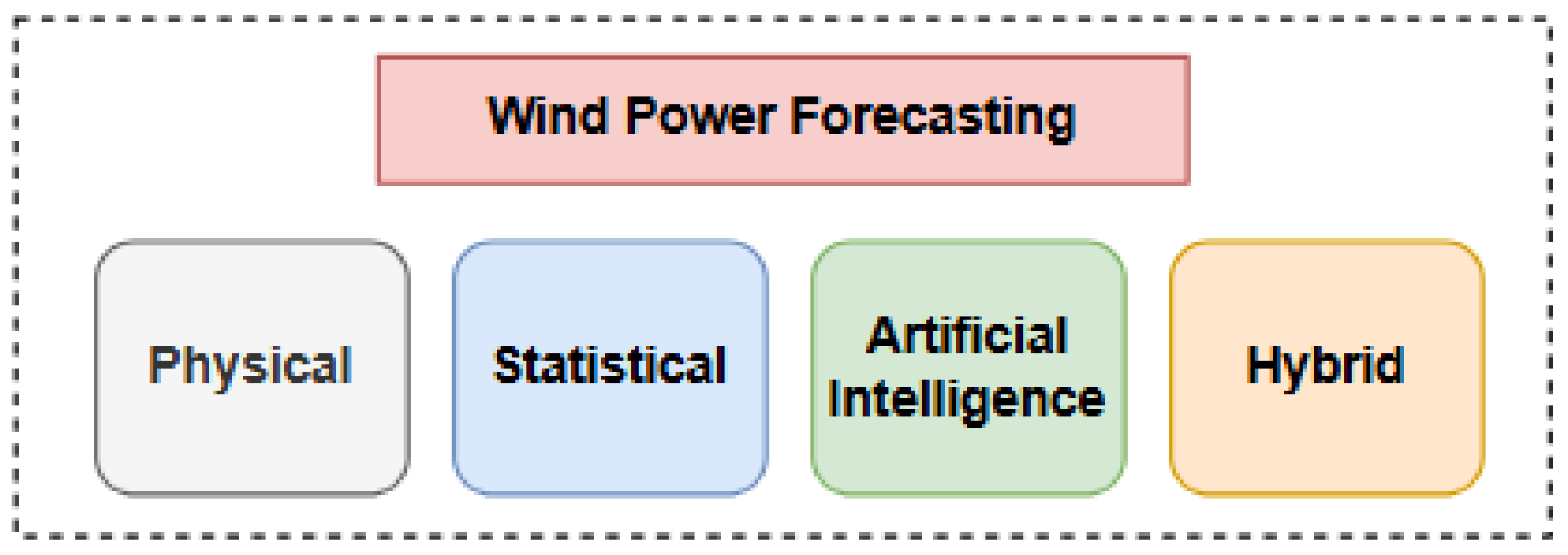
Due to the stochastic nature and variability of wind speed, different forecasting approaches have been proposed. In general, these models fall into four main categories: physical, statistical, Artificial Intelligence (AI) based models, and hybrid approaches [11], as illustrated in Figure 1. Each category has distinct characteristics, varying in computational cost, implementation complexity, and ability to capture specific data patterns, among other factors.

1.1. Literature Review

The most well-known physical models include the Numerical Weather Prediction (NWP) and the Weather Research and Forecasting (WRF) [12,13]. These models seek to predict wind speeds through complex mathematical formulas, involving meteorological factors such as air pressure, humidity, and temperature [14]. These models can be good for medium- and long-term forecasts. However, they have a very high computational cost, making them less viable for short-term local forecasts [15]. The most common statistical models are the autoregressive moving average (ARMA) [16], the autoregressive integrated moving average (ARIMA) [17], and the fractional ARIMA (f-ARIMA) [18]. They generally work well for short-term forecasts and may be viable for such applications. These models, which use historical wind speed data, are suitable for dealing with linear time series. However, such models often have certain limitations. Because they cannot effectively capture the non-linear information existing in wind speed data [14].

AI-based models generally focus on non-linear fluctuations in wind speed and have architectures more suited to sequence modeling issues, such as time series. Some classic AI-based models are the backpropagation neural network (BPNN) [19], multilayer perceptron (MLP) [20], support vector machine (SVM) [21], convolutional neural network (CNN) [22], recurrent neural network (RNN) [23], gated recurrent unit (GRU) [24], Long Short-Term Memory (LSTM) [25], and despite their success, these AI-based models still exhibit certain limitations. Traditional neural architectures such as MLP, CNN, RNN, LSTM, and GRU may struggle to capture long-term dependencies in sequential data and can suffer from issues like vanishing gradients or high computational cost when processing long sequences. Moreover, their limited ability to parallelize computations constrains scalability for large datasets.

To address these limitations, the Transformer architecture [26] has recently been applied to time series forecasting tasks. Originally developed for natural language processing, the Transformer model leverages attention mechanisms to capture long-range dependencies in sequential data more efficiently. Over time, this architecture has been adapted for time series applications, giving rise to several specialized variants such as the LogSparse Transformer [27], Temporal Fusion Transformer (TFT) [28], Informer [29], Reformer [30], Pyraformer [31], Autoformer [32], FEDformer [33], PatchTST [34], Crossformer [35], Flowformer [36], FlashAttention [37]. These models were developed to overcome some limitations of the original (vanilla) Transformer, which exhibits quadratic complexity due to the FullAttention mechanism. When applied to very long time series, this can result in high computational demands and reduced efficiency. Consequently, the newly developed variants offer improved efficiency and lower computational requirements, making them more suitable for forecasting long sequences. This topic will be discussed in more detail later in this study. In the scientific literature, both the Transformer model and its derivatives are commonly referred to as X-formers [38].

Due to the high complexity and fluctuations in wind speed, many studies state that a single model may not comprehensively describe these fluctuations. The adoption of hybrid models is necessary. According to Ref. [39], some important aspects for these models are data predictability and the selection of ideal hyperparameters, with appropriate optimization algorithms. Some examples of hybrid models are Bidirectional LSTM (BiLSTM) [40], CNN-LSTM [41], Spatial-Temporal Graph Transformer Network (STGTN) [42], among others.

1.2. Review of Transformer Applications in Wind Energy Forecasting

Several studies have applied Transformer architectures or models derived from them to forecast time series in wind energy, demonstrating strong performance. For instance:

• FFTransformer [43] incorporates signal decomposition through two streams to analyze trend and periodic components, while capturing spatio-temporal relationships. It outperformed LSTM and MLP in short-term wind speed and power forecasting.
• A hybrid model based on the Informer with the addition of a CNN [44] showed superior performance compared to LSTM for short-term wind power forecasting.
• Integration of the Transformer with wavelet decomposition [45] improved wind speed prediction at different heights, outperforming LSTM.
• In Ref. [46], the Transformer model was used with the addition of a method, the Improved Complete Ensemble Empirical Mode Decomposition with Adaptive Noise (ICEEMDAN). There was also the addition of a new kernel MSE loss function (NLF). The results showed the lowest errors for the proposed method compared to GRU, RNN, and others in wind speed forecasting.
• In Ref. [47], the authors proposed the VMD-Transformer (VMD-TF), a Transformer model combined with Variational Mode Decomposition (VMD), to mitigate the effects of wind speed non-stationarity by decomposing the signals into stable modes. The results demonstrated that the VMD-TF outperformed models such as VMD-ARIMA and VMD-LSTM in short-term forecasting.
• GAT-Informer [48], Integrates Graph Attention Networks (GAT) with Informer to capture spatial and temporal dependencies, outperforming reference models such as GRU.
• WindFix [49], a self-supervised learning framework based on the Transformer architecture and masking strategies, designed to impute missing values in offshore wind speed time series. The model adapts to various missing data scenarios, leverages spatiotemporal correlations, and achieves low mean squared error (MSE).
• In Ref. [50], the authors employed Informer for wind speed forecasting in combination with Wavelet Decomposition (WD), which was used to reduce high-frequency noise in the monitored wind speed signal series. The results demonstrate that the proposed model outperforms other approaches, including GRU and the standard Transformer.

1.2.1. Limitation of Transformer Models

Despite these promising results, Transformer-based models exhibit certain limitations in modeling temporal dependencies, particularly periodic, seasonal, and long-term patterns commonly found in time series:

• Positional encodings: The original Transformer uses fixed sinusoidal positional encodings, which are often insufficient to represent complex temporal dynamics. Mechanisms like Time2Vec [51] offer learnable temporal encodings that better capture periodic signals and cyclical behaviors, including daily and seasonal cycles. Studies integrating Time2Vec into Transformers, MLP, and LSTM [52] have reported improvements exceeding 20% in some forecast horizons.
• Computational complexity: The quadratic complexity of FullAttention limits scalability for long sequences. Efficient attention variants such as ProbSparse Attention, FlowAttention and FlashAttention significantly reduce complexity without sacrificing accuracy (further discussed in Section 2.4).
• Interpretability and novelty: Transformer-based models are still relatively new in the context of wind energy forecasting. While they have shown strong predictive performance, the internal workings of attention mechanisms and learned representations are not always straightforward to interpret. This inherent complexity can make it challenging to fully understand how the model arrives at specific predictions, particularly in operational settings.

1.2.2. Research Gaps and Motivation

Although various improvements exist, several gaps remain in the application of Transformers to wind energy forecasting:

• Integration: The effectiveness of integrating Time2Vec within specific components of the Transformer architecture—namely the encoder, the decoder, or both—has not been systematically investigated in the context of time series forecasting;
• Efficient attention mechanisms: Different attention mechanisms have not yet been systematically evaluated for short-term wind power forecasting, especially the FlashAttention mechanism.
• Combined Temporal Encoding and Attention Mechanisms: The joint evaluation of different attention mechanisms combined with temporal encodings such as Time2Vec has not yet been explored, particularly for short-term wind power forecasting.
• Computational efficiency: The runtime performance and scalability of Transformer variants, particularly those incorporating efficient attention mechanisms such as FlowAttention and FlashAttention, have not been thoroughly evaluated in the context of short-term wind power forecasting.

This study addresses these gaps by proposing and evaluating four Transformer-based models: T2V-Transformer, T2V-Informer, T2V-Flowformer, and T2V-Flashformer. Each architecture incorporates Time2Vec into a different attention mechanism, enabling a comparative analysis of forecasting accuracy and computational efficiency. Sensitivity and hyperparameter analyses are conducted to identify optimal configurations, emphasizing the novelty of jointly evaluating Time2Vec with efficient attention mechanisms for wind power forecasting.

1.2.3. Objective and Contributions

Accurate power generation forecasts are essential to maximize the operational efficiency of wind farms. Transformer-based models have demonstrated strong performance in this area, often surpassing classical time series models. Building on these advances, this work evaluates different Transformer-based architectures and recent variants for short-term wind power forecasting, with an emphasis on predictive accuracy and computational efficiency.

The main contributions of this study are as follows:

• We propose a modification to the original Transformer architecture by incorporating a Time2Vec layer, which replaces the traditional input embedding layer. This replacement enriches the input representations with temporal features, aiming to capture time-dependent patterns better. In addition, we conduct a sensitivity analysis to identify the configuration that best favors the model architecture;
• We introduce flexibility in model design by enabling the use of different attention mechanisms—replacing the traditional FullAttention with ProbSparse Attention, FlowAttention and FlashAttention, resulting in the proposed models T2V-Informer, T2V-Flowformer and T2V-Flashformer, alongside the baseline T2V-Transformer. This substitution reduces computational complexity and enhances efficiency;
• We perform an extensive comparison of the proposed architectures with their baseline counterparts (Transformer, Informer, Flowformer and Flashformer). To the best of our knowledge, this is the first study applying the FlashAttention mechanism to wind turbine power forecasting. Moreover, a comprehensive hyperparameter search was conducted to determine the optimal configuration for each model;
• The proposed models exhibit strong adaptability and can be effectively applied to a broad spectrum of time series forecasting tasks beyond wind power prediction;
• By evaluating model behavior across two distinct forecasting scenarios, this work also serves as a practical reference for researchers and practitioners, providing insights into how Transformer-based architectures perform under different conditions and guiding their effective deployment in wind power forecasting.

All of these contributions aim to improve time series forecasting to maximize the energy efficiency of production systems.

Beyond combining Time2Vec and efficient attention mechanisms, this study introduces an integrated architecture where continuous temporal encoding interacts directly with attention computation. This design enhances the model’s ability to capture periodic dependencies while reducing computational and memory costs. The integration provides both architectural and empirical advances, leading to improved interpretability and superior forecasting performance compared to baseline models.

1.3. Sections

The remainder of this paper is organized as follows. Section 2 presents the Theoretical Foundation upon which this work is based. Section 3 discusses the Methodology adopted for conducting the experiments. Section 4 presents the Results and a detailed Discussion of the experiments, based on the methodology and techniques employed in this study. Section 5 concludes the paper. Section 6 presents Future Perspectives. Appendix A presents the results of the sensitivity analysis conducted in this study.

2. Theoretical Foundation

The objective of this section is to present the models used for power forecasting in time series, focusing on the MLP, LSTM, DLinear, Transformer, Informer, Flowformer, and Flashformer models. This section is crucial to the paper, as it lays the theoretical foundation for the comparative analysis of these models, highlighting the advantages and limitations of each approach. By concentrating on Transformer models and their derivatives with the addition of Time2Vec, the aim is to investigate improvements in accuracy and computational efficiency, thereby linking classical models with the innovations proposed in this work.

For comparison purposes, models representing distinct approaches to time series forecasting were selected: MLP, as a baseline dense neural network; LSTM, as a recurrent model widely used for energy forecasting; DLinear, as a recently proposed efficient linear model for time series; and Transformer, Informer, Flowformer, and the variant employing the FlashAttention mechanism (referred to as Flashformer in this study), as representatives of attention-based architectures. This selection aims to cover a representative spectrum of model complexity, temporal dependency modeling capability, and computational cost.

2.1. Multi-Layer Perceptron

The Multi-Layer Perceptron (MLP) is a deep learning model that consists of multiple layers of nodes (neurons). These layers are feedforward networks that learn weights Θ, and map the input to the output Ө and map the input to the output $y\approx f(x|\mathsf{Ө}).$ The network forms a layered structure, where several layers are stacked, giving depth to the model. Therefore, the output is characterized by Equation (1) below:

$$\widehat{y}=f^{\left(n+1\right)}\left(f^{\left(n\right)}\left(\dots f^{\left(2\right)}\left(f^{\left(1\right)}\left(x|{\mathsf{Ө}}_1\right)|{\mathsf{Ө}}_2\right)\dots |{\mathsf{Ө}}_n\right)|{\mathsf{Ө}}_{n+1}\right)$$

(1)

where $f^{\left(1\right)}$ represents the transformation applied by the first hidden layer, with weight ${\mathsf{Ө}}_1$, $f^{\left(2\right)}$ by the second hidden layer, with weight ${\mathsf{Ө}}_2$. $f^{\left(n\right)}$ by the nth hidden layer, with weight ${\mathsf{Ө}}_n$. E $f^{\left(n+1\right)}$ for the last hidden layer, with weight ${\mathsf{Ө}}_{n+1}$. The Equation (3) represents how the input x is progressively transformed through the n hidden layers, and finally mapped to the output layer $\widehat{y}$ [53].

MLP is a fundamental neural network architecture characterized by its simplicity and ease of implementation, which makes it suitable for a broad range of supervised learning tasks, including classification and regression. Nevertheless, its feedforward structure presents inherent limitations when applied to complex datasets, particularly in capturing long-term temporal dependencies.

2.2. Long Short-Term Memory

LSTM is a Recurrent Neural Network (RNN) designed for sequence learning. Unlike traditional RNNs, LSTMs can learn long-term dependencies and mitigate the “gradient vanishing” problem that hinders effective learning during backpropagation. LSTMs employ control gates to manage information flow: the input gate determines what information to add to the memory cell, the forget gate decides what to discard, and the output gate selects the information to use at any given moment, optimizing model efficiency [54].

LSTM is characterized by its strong ability to capture long-term dependencies and identify complex temporal patterns. Its limitations include relatively high computational complexity, the need for large datasets, and the risk of overfitting.

2.3. DLinear

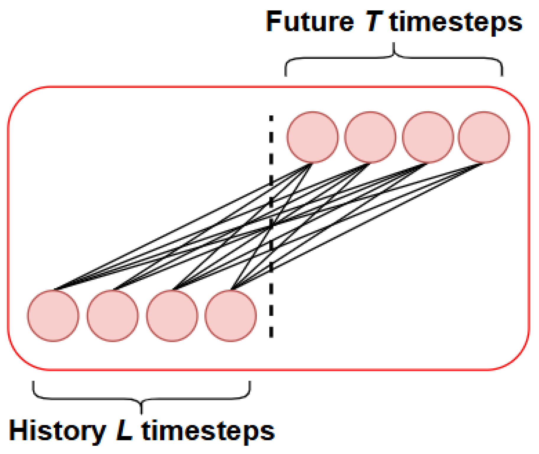
The DLinear model [55] adopts a linear approach for time series forecasting, emphasizing simplicity and computational efficiency. Unlike Transformer-based architectures, which rely on complex attention mechanisms, DLinear is built upon the assumption that time series can be effectively represented through linear relationships. This model was proposed to question the effectiveness of Transformers for time series forecasting due to their high computational cost, inefficiency, and potential for overfitting, particularly in long sequences. DLinear consists of multiple linear layers applied across the temporal dimension, preserving linearity throughout its transformations. Two variants were proposed: NLinear and DLinear, both of which perform time series regression through a weighted summation operation, as illustrated in Figure 2. Formally, the forecasting process can be expressed as $\widehat{X}=W{X}_i$, where $W$ $\in$ $R^{T.L}$ is a learnable weight matrix, $\widehat{X}$ denotes the forecast, and $X_i$ is the input for the n-th variable.

For this study, the DLinear variant was selected, which was specifically designed for time series across different domains. It separates the trend and seasonality components: the trend captures long-term patterns, while seasonality captures repetitive short-term patterns. A simple linear regression is applied to each component. Limitations of DLinear include difficulty capturing specific patterns in complex time series.

2.4. Transformer

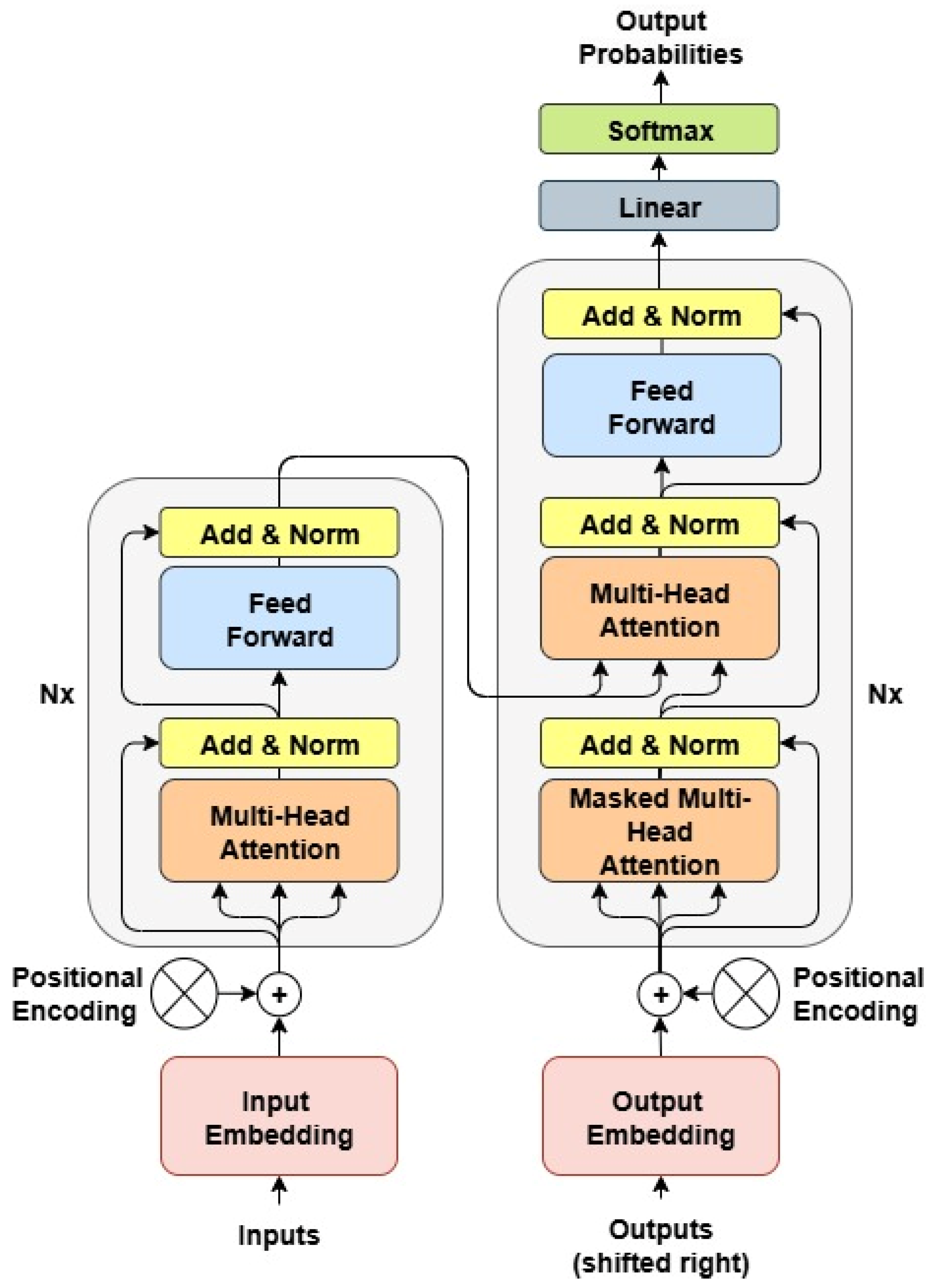
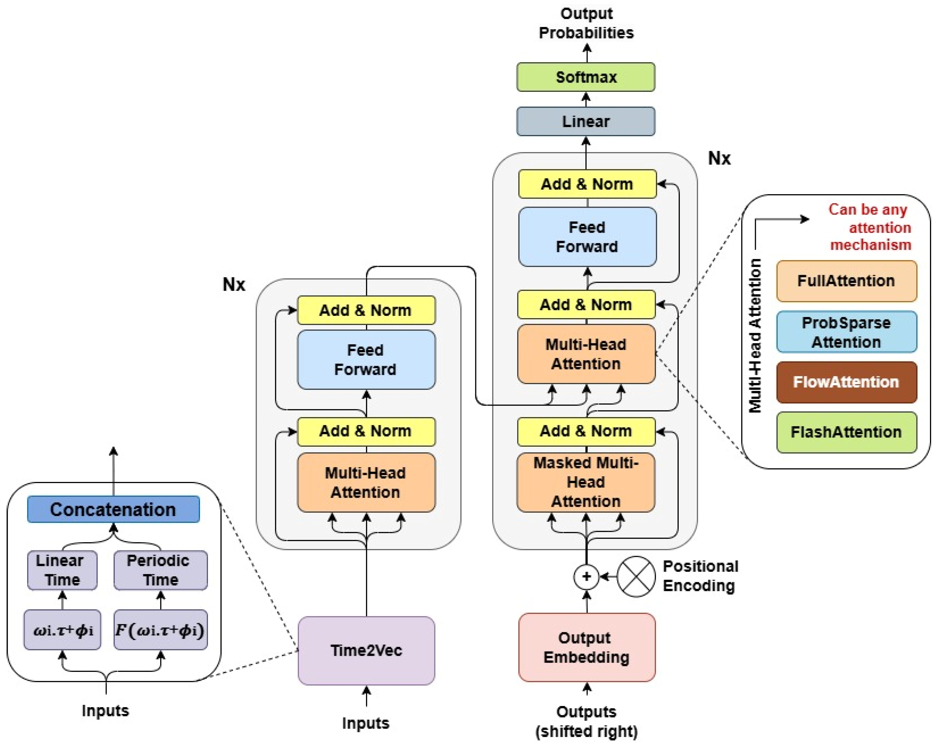
Transformers are deep learning neural networks originally designed for NLP [56]. Figure 3 shows the first model, known as the Vanilla Transformer [26], which consists of an encoder-decoder architecture using stacked self-attention and fully connected layers. Each encoder consists of two main sublayers: (I) a multi-head self-attention mechanism, and (II) a position-wise feed-forward neural network. Both sublayers are followed by residual connections and layer normalization (‘Add & Norm’). The input embeddings are combined with positional encodings to retain sequence information before being fed into the encoder. The decoder, on the right side of Figure 3, includes three sublayers: (I) a masked multi-head self-attention layer that prevents the decoder from attending to future positions, (II) a multi-head attention layer over the encoder’s output (enabling interaction between encoder and decoder), and (III) a feed-forward neural network. Similarly, residual connections and normalization are applied after each sublayer. The output embeddings are also combined with positional encodings and shifted to the right to ensure autoregressive decoding. Finally, the decoder output is passed through a linear transformation and a SoftMax layer to generate output probabilities.

Multi-head attention uses the query Q, key K, and value V vectors to compute outputs by weighting the values based on the relevance between queries and keys. The Scaled Dot-Product, attention mechanism, formalized Equation (2), is used to derive the context vector by calculating the similarity between Q and K, scaling it, and applying it to V.

$$\mathrm{Attention}\left(Q,K,V\right)=softmax\left({\displaystyle \frac{Q{K}^T}{\sqrt{D_K}}}\right)V$$

(2)

The model receives the input sequence x = {x₁,…, x_n} and generates the representations Q, K, and V through linear transformations, defined as $Q = W^{Q}x$; $K = W^{K}x$ and $V = W^{V}x$, where $W^Q$, $W^K$ e $W^V$ are learnable weight matrices.

The Transformer architecture applies multi-head attention, enabling the model to attend to information from different representation subspaces at other positions. Instead of performing a single attention function with dimensions $d_{model}$, the model projects Q, K, and V linearly h times into dimensions $d_k$, $d_k$, and $d_v$, respectively. Each projected version of Q, K, and V undergoes an independent attention operation, performed in parallel, producing h outputs of dimension $d_v$.

These outputs are concatenated and passed through a final linear projection, resulting in the Multi-Head Attention output, as shown in Equation (3). Each $hea{d}_i$ is individually computed using the Scaled Dot-Product Attention mechanism, as defined in Equation (4):

$$MultiHead\left(Q,K,V\right)=Concat\left(hea{d}_1, \dots , hea{d}_h\right)W^0$$

(3)

$$hea{d}_1=Attention(Q{W_i}^Q, K{W_i}^K \mathrm{e} V{W_i}^V)$$

(4)

The projection matrices are $W_i$^Q ∈ $R^{d_{model}.d_K}$, $W_i$^K ∈ $R^{d_{model}.d_K}$, and $W_i$^V ∈ $R^{d_{model}.d_V}$ for each $hea{d}_i$, and $W^0$ ∈ $R^{h{d}_V.d_{model}}$ for the output projection. Here, $d_{model}$ denotes the model dimension, $h$ is the number of attention heads, and typically $d_K=d_V=$ $d_{model}$/h. This mechanism is commonly referred to as FullAttention.

The Feed Forward sublayers (see Figure 3), with dimensions $d_{ff}$, consist of two linear transformations separated by a non-linear activation function. The first transformation outputs a dimension o $d_{model}$, which is then projected to $d_{ff}$ (usually larger than $d_{model}$). The activation function enables the model to learn complex functions, and the second transformation projects the output back to $d_{model}$. Suggested values for these variables can be found in Ref. [26].

In order to retain information about the sequential order of the inputs, the Transformer incorporates positional encodings into the input embeddings before they are processed by the encoder. These encodings provide each position in the sequence with a unique representation based on sinusoidal functions of different frequencies, as formalized in Equation (5):

$$P{E}_{\left(pos,2i\right)}=\sin \left({\displaystyle \frac{pos}{{\mathrm{10,000}}^{2i/d_{model}}}}\right), P{E}_{\left(pos,2i+1\right)}=\cos \left({\displaystyle \frac{pos}{{\mathrm{10,000}}^{2i/d_{model}}}}\right)$$

(5)

where $pos$ is the position index and i is the dimension index of the embedding vector. These sinusoidal encodings enable the model to infer relative positions between tokens through linear combinations of the input embeddings. Similarly, the decoder input embeddings are combined with the same positional encodings (Equation (5)) before being processed by the masked self-attention layer, ensuring consistent positional information across both encoder and decoder components [26].

According to Equation (2), attention results from the dot product $Q{K}^T$, yielding a scoring matrix of size N × N with a computational cost of O($N^2$·d), where d is the embedding dimension and N is the sequence length. The softmax function applied to O($N^2$·d) amplifies the quadratic complexity issue. As N increases, the number of required operations grows quadratically, making long sequence processing costly in time, computation, and memory. Several studies have been conducted to mitigate these limitations and refine the Transformer architecture.

To overcome these limitations, several variants have been proposed, focusing on improving efficiency, scalability, and temporal representation learning. These aspects are discussed in more detail below.

2.4.1. Informer

The Informer model [29] addresses the quadratic computational complexity of the Vanilla Transformer in long-sequence forecasting tasks. It introduces the ProbSparse Self-Attention mechanism, which identifies and retains only the most informative queries, reducing redundancy in attention computation. By focusing on a sparse subset of queries, the overall complexity is reduced from O(N²) to approximately O(N Log N). Formally, the attention mechanism is defined in Equation (2); however, in ProbSparse Attention, only the dominant queries with the highest information contribution are retained, improving efficiency without significant accuracy loss.

Informer also employs a self-attention distilling operation, implemented through max-pooling layers in the encoder. This process compresses attention maps between layers, preserving essential temporal dependencies while filtering out redundant or noisy information. The distilling mechanism enhances both memory efficiency and the model’s ability to generalize to long input sequences. Additionally, Informer replaces the traditional autoregressive decoder with a generative-style decoder, enabling the prediction of the entire future sequence in a single forward pass. These innovations make Informer highly scalable and effective for long-term time series forecasting, combining reduced computational cost, lower memory demand, and competitive predictive accuracy [29].

2.4.2. Flowformer

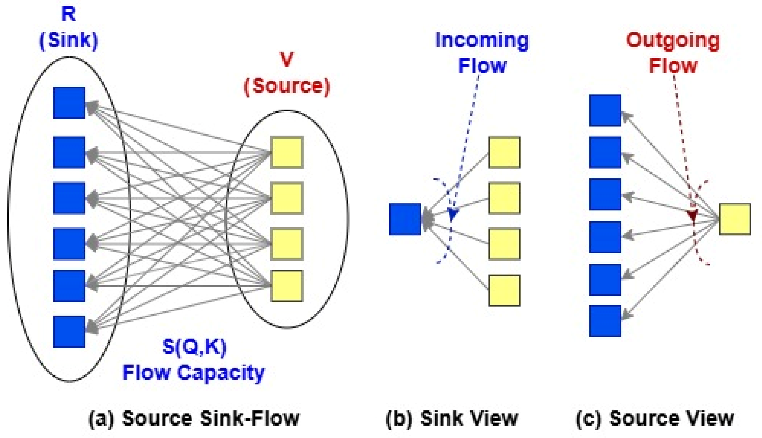
The Flowformer model [36] reduces the quadratic complexity of Transformers by using flux conservation principles. It redefines the attention mechanism from the perspective of flow networks, achieving approximately linear complexity, O(N) (see Figure 4). In (a), the blue squares represent R (Sink), while the yellow squares represent V (Source). The concept of flow originates from transportation theory, where input tokens are treated as sources and sinks connected by a flow with capacity determined by the matrix S(Q, K). This matrix defines the amount of flow that can be transported between each pair of tokens, similar to the attention computation in conventional Transformers. In (b), it is observed that each sink token (blue) receives flow from multiple source tokens (yellow). In (c), each source token (yellow) distributes its flow to multiple sink tokens (blue). In traditional Transformers, the results R are derived from the values V, weighted by attention scores that depend on the similarity between the query Q and the key K. In the Flowformer model, R acts as collectors receiving information from V, which serve as sources. The attention weights, represented as flow capacities, are computed based on Q and K. Here, attention is formulated as a transportation problem where Q and K are treated as probability distributions. The optimal solution to this problem defines the attention mechanism, referred to as FlowAttention. Consequently, the dot product $S=Q{K}^T$ in the Vanilla Transformer is replaced by $S=\varphi \left(Q\right)\varphi \left(K^T\right)$, where $\varphi \left(·\right)$ is a non-linear function ensuring that the positive properties of flow networks are preserved.

2.4.3. FlashAttention

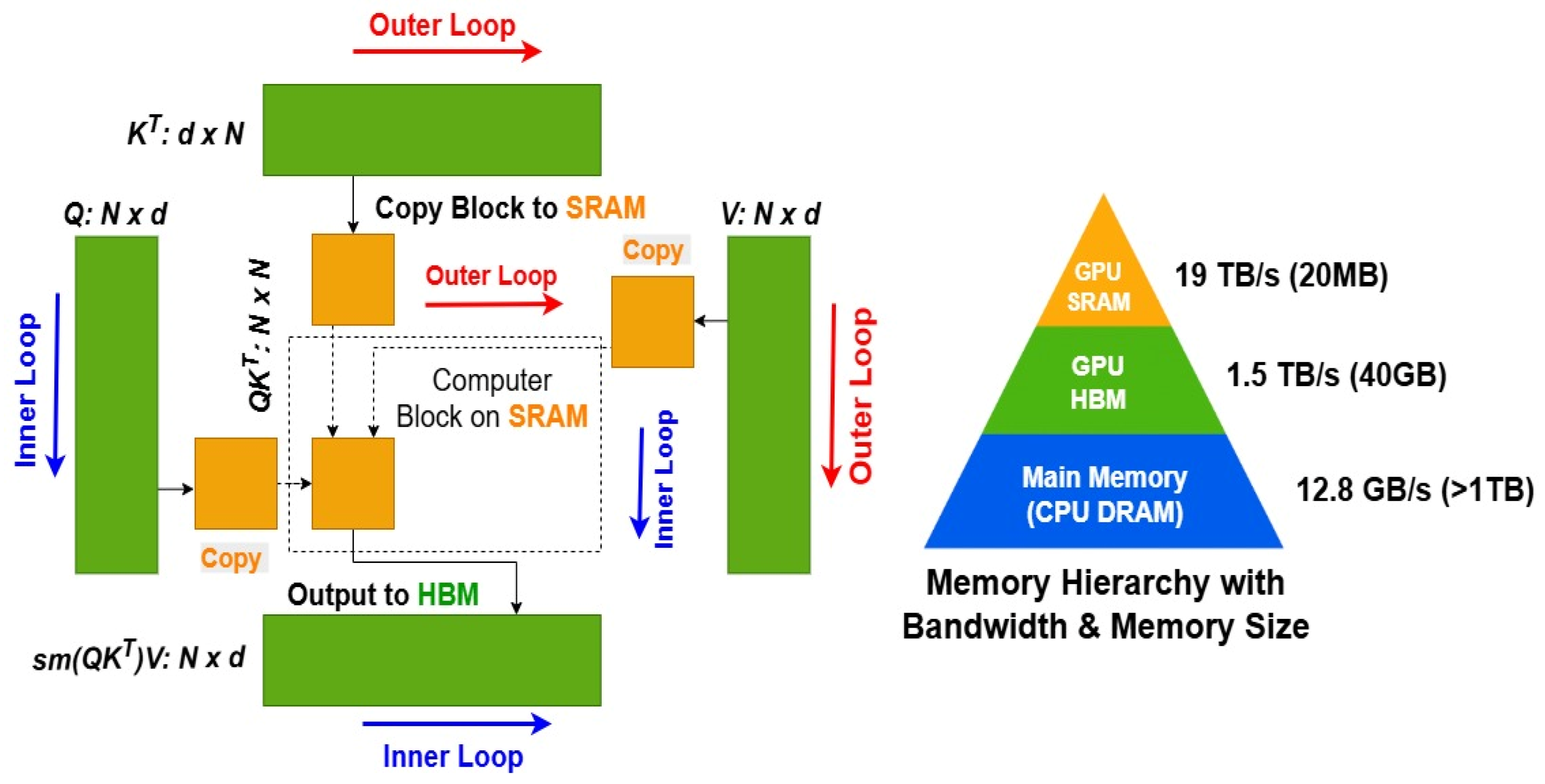
The model is optimized for time series forecasting and incorporates a memory-efficient attention mechanism with I/O awareness. Using the FlashAttention algorithm [37] minimizes the number of read and write operations between the high-bandwidth memory (HBM) and the on-chip static random-access memory (SRAM) of the GPU. As illustrated in Figure 5, FlashAttention processes tokens within a sliding window to capture local dependencies, which are essential in time series modeling. The algorithm employs a tiling strategy to avoid the explicit materialization of the full N × N attention matrix (dotted box) in the relatively slow GPU HBM. In the outer loop (red arrows), FlashAttention iterates over blocks of the K and V matrices, loading them into the fast on-chip SRAM. Within each block, it loops over segments of the Q matrix (blue arrows), loading them into SRAM and writing the resulting attention outputs back to HBM. Although the arithmetic complexity remains O($N^2)$, FlashAttention substantially reduces I/O complexity by limiting memory traffic between HBM and SRAM. Heuristically, this reduction can be approximated as O($N^2/M)$, where M represents the effective on-chip memory capacity. The exact efficiency gain depends on the block size and hardware configuration. FlashAttention can directly replace the standard FullAttention mechanism in the Vanilla Transformer. In this study, the Transformer variant employing FlashAttention is referred to as Flashformer.

2.4.4. Overview of Transformer-Based Models

The Informer extends the Vanilla Transformer by improving scalability through sparse attention and encoder distillation, reducing computational complexity to approximately O(N Log N) while maintaining forecasting accuracy. The Flowformer, on the other hand, introduces a flow-based decomposition of attention, which can reduce redundant computations but may occasionally increase complexity beyond O(N) depending on the dimensionality of the flow representation and the implementation details. The Flashformer leverages FlashAttention, which performs attention computation in a memory-efficient manner by optimizing GPU caching and parallelism. However, its performance strongly depends on specialized hardware (e.g., CUDA-enabled GPUs) and implementation parameters (e.g., block size and tiling strategy), which can affect its effective runtime complexity. The choice of the most suitable model depends on the specific application.

Table 1. Summary and overview of each model.

Model	Attention Mechanism	Complexity
Transformer	FullAttention	O(N2)
Informer	ProbSparse Attention	O(N Log N)
Flowformer	FlowAttention	O(N)
Flashformer	FlashAttention	O(N2/M) 1

¹ Approximate complexity, see Ref. [37] for details.

summarizes the X-former models employed in this study, highlighting their respective attention mechanisms and computational complexities.

In summary, these models represent different trade-offs between computational efficiency and representational capacity. Vanilla Transformer offers robust performance but exhibits moderate scalability with input length due to its quadratic complexity. The Informer improves scalability through sparse attention, reducing computational cost. However, its probabilistic query selection may fail to capture certain long-range dependencies, potentially leading to slight accuracy degradation in some forecasting scenarios. The Flowformer improves scalability for longer sequences, potentially enhancing performance in high-frequency or large-scale wind datasets. The Flashformer, in turn, emphasizes runtime efficiency, enabling faster training and inference on modern GPU architectures. Therefore, evaluating these models under a unified framework is essential to determine which mechanism—standard, flow-based, or hardware-optimized attention—best balances accuracy and computational cost for short-term wind power forecasting.

2.5. Time2Vec: Learning a Vector Representation of Time

Feature learning aims to automatically extract informative representations from raw data, enhancing model performance by capturing underlying structures and dependencies. In the context of time series forecasting, temporal representation learning plays a crucial role in enabling models to understand periodicity and temporal dynamics effectively. Among the existing approaches, Time2Vec [51] stands out as a simple yet powerful technique for encoding time-related information. It provides a systematic way to represent both periodic and non-periodic components of temporal data, offering a richer and more interpretable temporal embedding for neural network architectures. Time2Vec adopts three key properties:

• Periodicity: It captures both periodic and non-periodic patterns in the data.
• Time-scale invariance: The representation remains consistent regardless of time-scale variations.
• Simplicity: The time representation is designed to be simple enough for integration into various models and architectures

Thus, instead of applying the dataset directly to the model, the authors propose that the original time series be transformed using the following representation by Equation (6):

$$\mathrm{t}2\mathrm{v}(\tau )[i] = \left\{\begin{array}{c}{\omega }_i · \tau + {\varphi }_i, \mathrm{if} i = 0\\ F \left({\omega }_i · \tau + {\varphi }_i\right), \mathrm{if} 1 \le i \le k\end{array}\right.$$

(6)

where k denotes the Time2Vec dimension, τ is a raw time series, F denotes a periodic activation function, and ω and ϕ denote a set of learnable parameters. The index i ∈ [0,k] corresponds to the position within the Time2Vec embedding dimension. F is typically a sine or cosine function that enables the model to detect periodic patterns in the data. Simultaneously, the linear term (i = 0) captures the progression of time, allowing the representation to model non-periodic and time-dependent components in the input sequence.

Time2Vec is a powerful technique that improves forecasting models, especially in problems with complex temporal variables. Its main advantage is how it represents time, allowing models to capture seasonal and periodic patterns effectively. Instead of using a simple or linear time representation, Time2Vec uses trigonometric functions to create a vector that captures the nuances of periodicity and seasonality in the data. Another important feature of Time2Vec is its ability to expand temporal input, generating multiple features that represent time at different scales. This gives the model a more detailed understanding of the temporal context, improving its predictive power. By integrating Time2Vec, models can better capture temporal dynamics, leading to more accurate forecasts in various applications. For wind power time series, it has demonstrated good results with its application together with LSTM and Deep Convolutional Neural Networks with Wide First-layer Kernels (WDCNN) [57].

3. Methodology

3.1. Problem Description

Short-term wind power forecasting presents challenges due to the stochastic and non-stationary nature of wind behavior. To address these characteristics, this study adopts Transformer-based models enhanced with mechanisms better suited to time series data. As discussed in previous section, conventional Transformer architectures face limitations related to fixed positional encodings, high computational complexity and limited interpretability. To overcome these issues, the ProbSparse Attention, FlowAttention and FlashAttention mechanisms are used to replace the traditional FullAttention, reducing computational cost and improving scalability. Additionally, a Time2Vec encoding layer is incorporated into the input pipeline to provide a richer representation of temporal patterns. These modifications aim to enhance predictive performance and computational efficiency, while also providing the basis for a more reliable interpretation of the data.

3.2. Method Overview

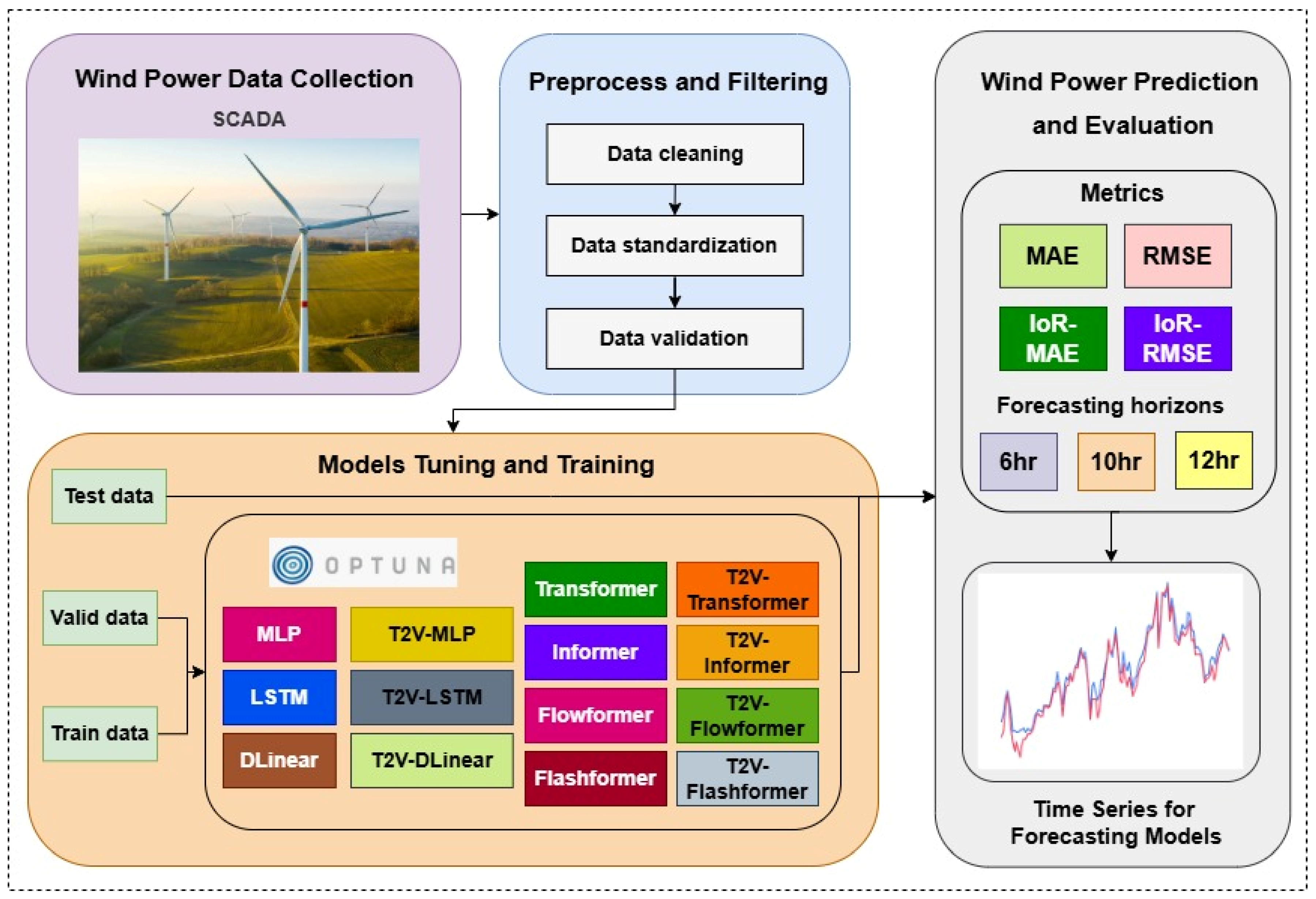
This study aims to forecast short-term wind power based on real operational data from wind turbines, addressing the challenges of accurate and timely energy prediction. This section details the methodological process adopted in this study, as summarized in Figure 6, based on the proposed framework.

The first stage involves the collection of data from operational wind turbines through the Supervisory Control and Data Acquisition (SCADA) system. To ensure data quality, the second stage involves preprocessing and filtering procedures, including data cleaning, outlier removal, and time series standardization to reduce noise and facilitate models training. Outlier removal was performed through local quality tests applied to the observed wind power data from the analyzed turbine. These hierarchical tests aimed to verify the physical and statistical consistency of the variable and to detect short-term abnormal behaviors, including range check, persistence check, and short-term step check. Missing data were handled through interpolation to maintain the temporal continuity and overall consistency of the time series prior to model training. These steps ensured that the dataset was properly scaled and consistent across all variables (the variables and their respective units are detailed in Section 3.5). Finally, the processed data are validated and prepared for use in the subsequent stage.

The third stage focuses on the adjustment and training of the models employed in this study. The models used include MLP, LSTM, DLinear, T2V-MLP, T2V-LSTM, T2V-DLinear, Transformer, Informer, Flowformer, and Flashformer, as well as the proposed models T2V-Transformer, T2V-Informer, T2V-Flowformer and T2V-Flashformer. The term T2V refers to the incorporation of the Time2Vec layer into the respective models. Furthermore, the trivial reference model called Persistence [58] was also used. The Persistence model, often used as a benchmark in time series forecasting, assumes that the value of the variable at a given time t will be equal to the value observed at time t − 1. In other words, the forecast for the next point in the series is the currently observed value. The third stage involves dividing the dataset into training, validation, and testing sets.

As shown in Figure 6, Optuna [59] was adopted as a tool for hyperparameter optimization of the models. During the training phase, the models receive data and adjust their parameters based on the information provided, learning patterns and relationships within the data. The models were trained using the Mean Squared Error (MSE) loss function, defined in Equation (7):

$$Loss = {\displaystyle \frac{1}{n}}{{\displaystyle \sum }}_{i=1}^n{\left(y_i-{\widehat{y}}_i\right)}^2$$

(7)

where $y_i$ denotes the actual value, ${\widehat{y}}_i$ represents the predicted value, and $n$ is the total number of samples in the batch. This objective function measures the average squared difference between predictions and targets. The optimizers used in the hyperparameter search were Adam [60], Root Megan Square Propagation (RMSprop) [61] and Stochastic Gradient Descent (SGD) [62], in order to enhance convergence robustness and mitigate the risk of overfitting. Early stopping was employed to halt training once validation performance ceased to improve, with a patience value of 5 applied across all simulations. The validation phase involves hyperparameter search to identify the optimal configuration for each model. In the testing phase, the trained and optimized models are evaluated using the test data to assess their performance in real-world scenarios.

The fourth step involves forecasting and evaluating the models based on the metrics described in Figure 6, for reference horizons of 6, 10, and 12 h ahead—which correspond to intra-day forecasting. This task is characterized as short-term forecasting. In the context of wind energy, short-term forecasting typically covers horizons of a few hours ahead and is widely addressed in the scientific literature. For instance, in Ref. [44], the authors performed predictions up to 3 h ahead; in Ref. [43], the predictions extended up to 4 h ahead; and in Ref. [45], the wind speed was predicted up to 6 h ahead. Therefore, the adopted horizons (6, 10, and 12 h) align with the operational definition of short-term forecasting and allow a consistent comparison with related works in the literature.

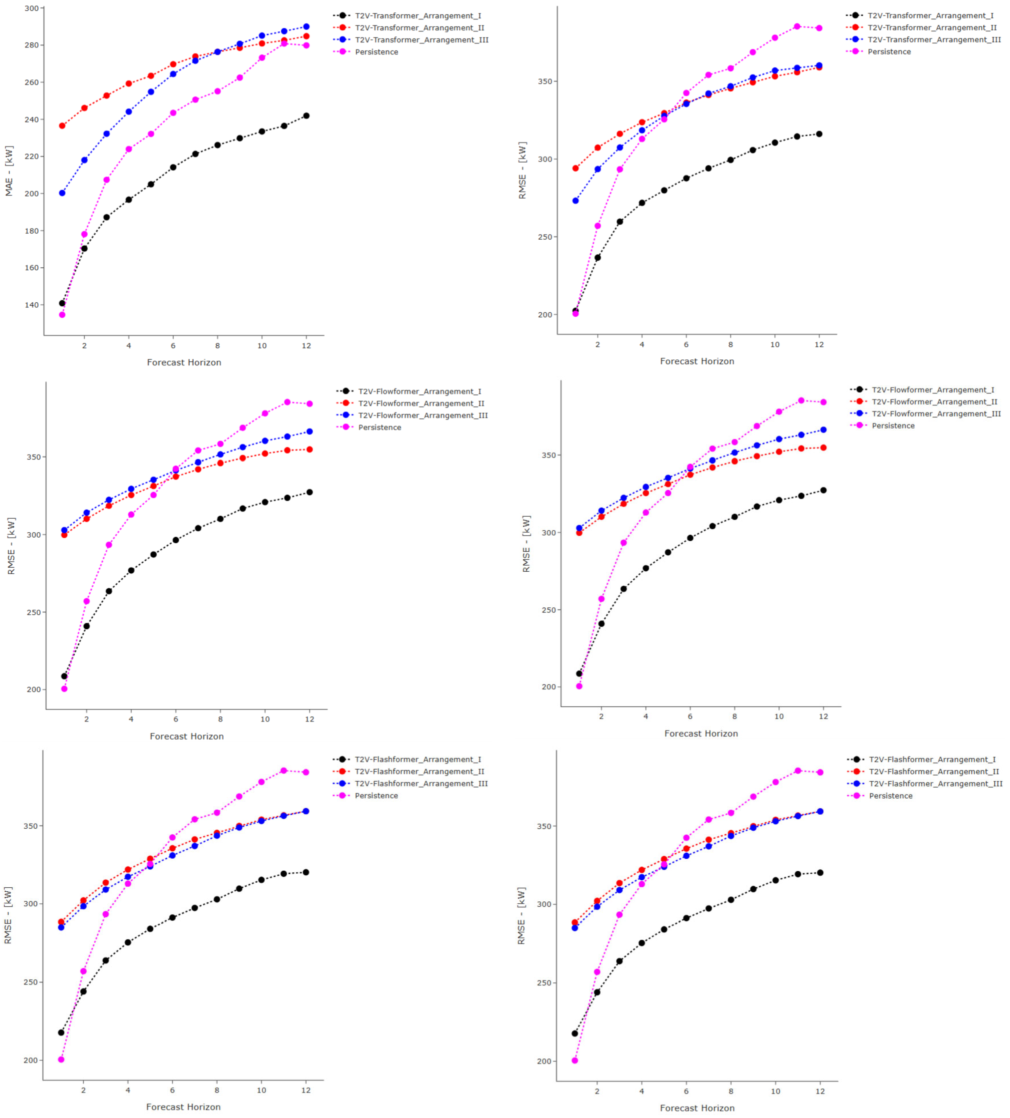
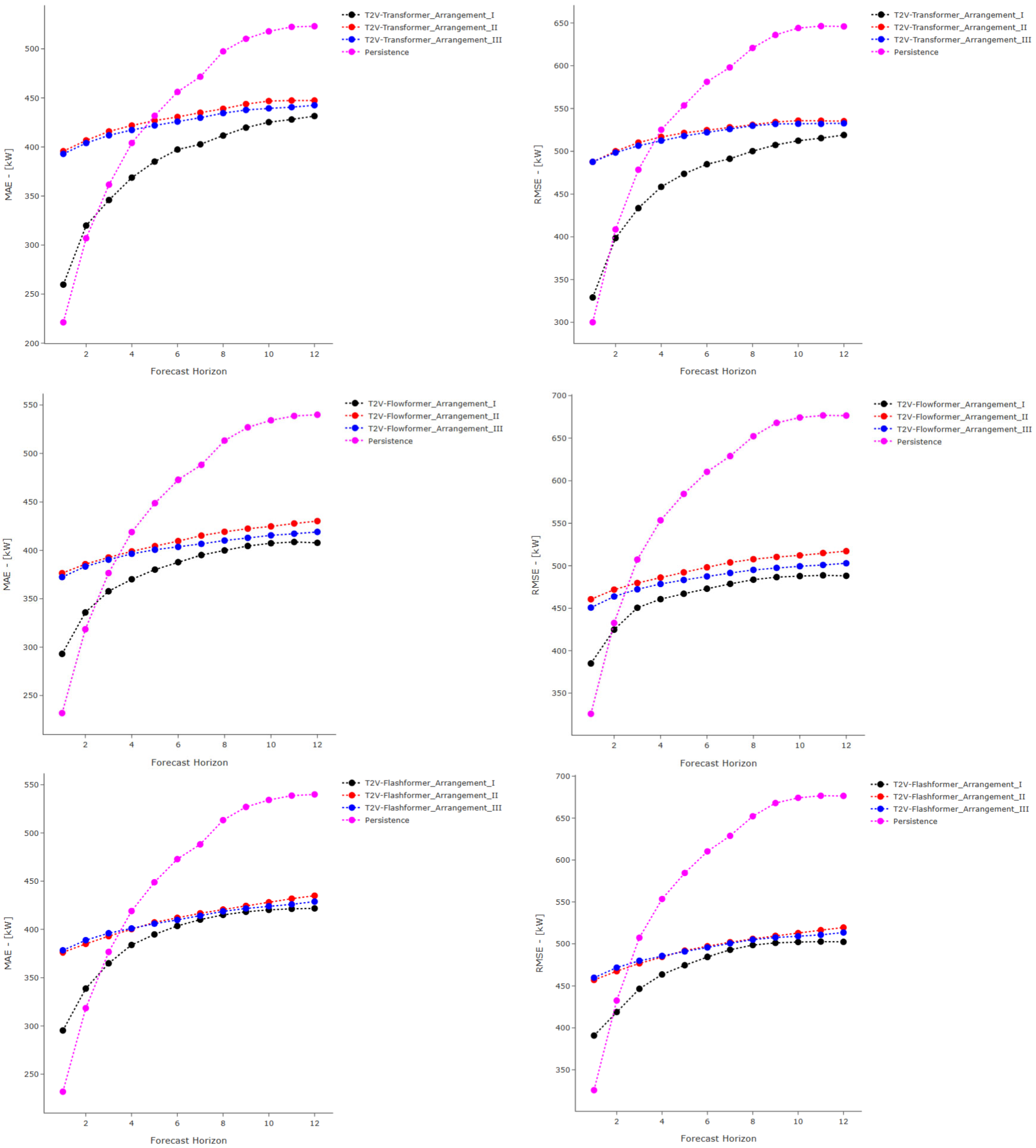
For the proposed models, a sensitivity analysis was conducted to determine the most effective configuration for integrating the Time2Vec mechanism into the Transformer architecture.

3.3. Sensitivity Analysis

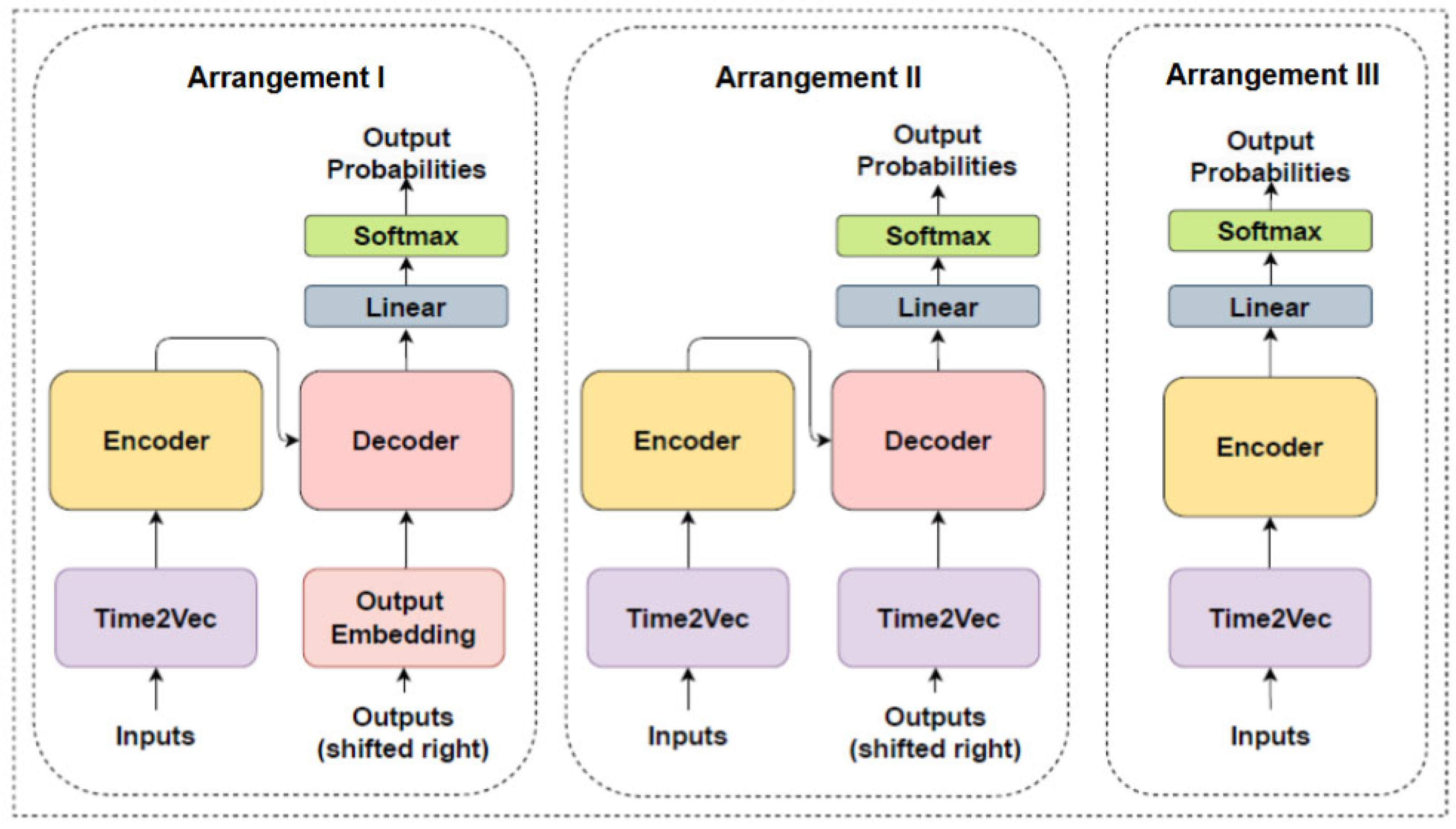
To integrate Time2Vec into the Transformer architecture, three distinct arrangements were explored to identify the one that most effectively enhances the architecture for wind power forecasting time series. The sensitivity analysis is presented in Figure 7. The following arrangements are described below:

• Arrangement I: employs both the encoder and the decoder, with Time2Vec added exclusively to the encoder input.
• Arrangement II: utilizes both the encoder and decoder, with Time2Vec incorporated into both the encoder and decoder inputs.
• Arrangement III: uses only the encoder, without the decoder, with Time2Vec applied to the encoder input

As far as the scientific literature indicates, this is the first time that such a specific sensitivity analysis has been conducted on the integration of Time2Vec into the Transformer architecture. The results obtained from the experiments, as presented in Appendix A, indicate that Arrangement I provided the most favorable conditions for the model’s performance. This configuration achieved the highest performance according to the evaluation metrics employed in this study. Therefore, this was the arrangement adopted for the models proposed in this study. The addition of Time2Vec only in the encoder allowed the model to learn temporal patterns more efficiently. The decoder, in turn, focuses on generating the output based on these representations, without the need to incorporate temporal information again. This approach thus avoids unnecessary complexity while maintaining optimized performance. However, removing the decoder from the model architecture compromised the model’s ability to generate predictions properly, as the decoder is crucial for transforming encoded representations into predictable outputs. The Time2Vec layer was also implemented in the MLP, LSTM, and DLinear models. This was done to verify how the layer behaves with other architectures and to assess its potential for improving performance across a range of model types. The T2V-DLinear model, which introduces the Time2Vec layer into the DLinear architecture, represents a novel approach in the scientific literature. While the primary focus of this study is on the integration of Time2Vec into Transformer-based models, T2V-DLinear serves as an additional benchmark to demonstrate the versatility of Time2Vec across different architectures.

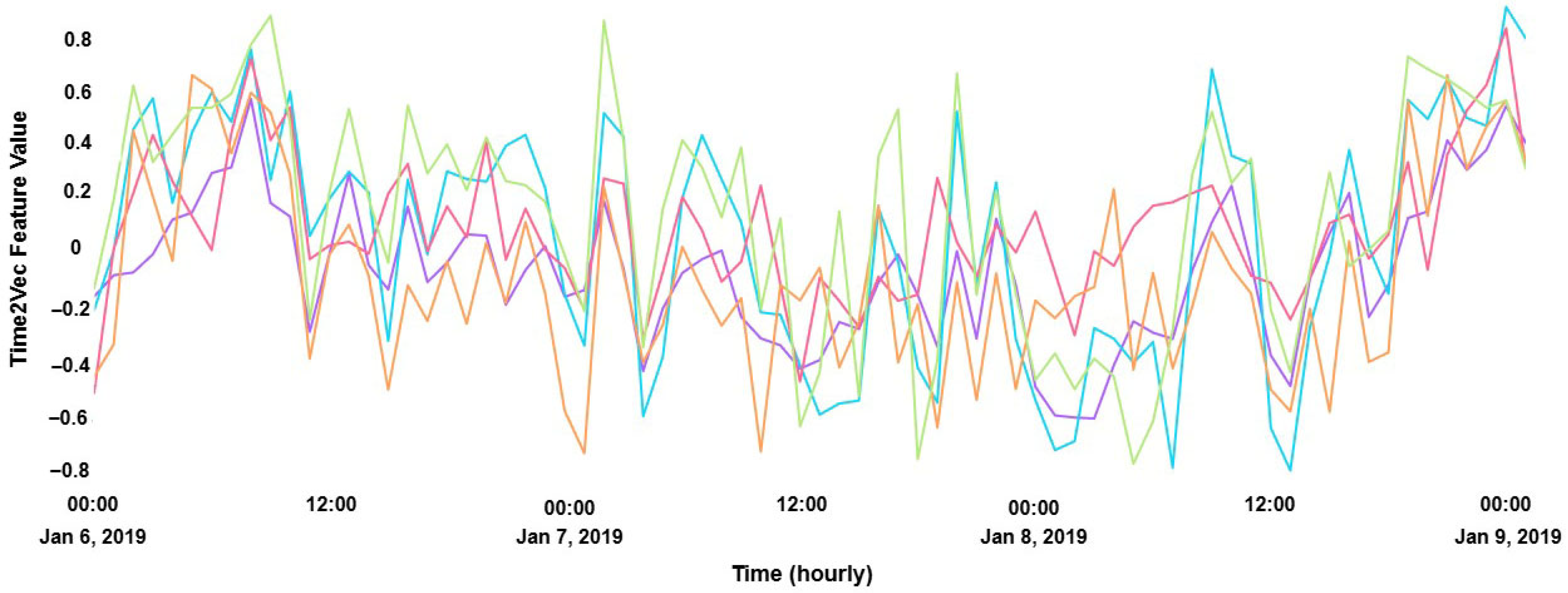
To better understand how the Time2Vec mechanism captures temporal dynamics, Figure 8 presents the learned embeddings generated by the Time2Vec layer after training on the wind energy time series. Each curve represents a distinct temporal dimension, illustrating how the model encodes periodic and trend-related patterns. The figure depicts a three-day segment of the time series, between 6–9 January 2019.

3.4. Proposed Models

The proposed changes to the Transformer architecture refer to Arrangement I, shown in the previous section. Furthermore, the classic attention mechanism known as FullAttention was replaced by the ProbSparse Attention, FlowAttention and FlashAttention mechanisms. The proposed model is illustrated in Figure 9. Any of these attention mechanisms can be adopted. The models that use FullAttention, ProbSparse Attention, FlowAttention, and FlashAttention in this work are called T2V-Transformer, T2V-Informer, T2V-Flowformer, and T2V-Flashformer, respectively. The proposed models underwent the sensitivity analysis described in Section 3.3. They follow the classic encoder-decoder architecture, with the flexibility to modify the attention mechanism, as illustrated in Figure 9.

In this study, the equations that define the attention computation (Equations (2)–(4)) follow the standard Transformer formulation [26]. However, specific adaptations were introduced to tailor them to the forecasting task and the Transformer-based architectures employed. In particular, the Time2Vec embeddings were integrated into the encoder inputs to provide explicit temporal information to the model, without modifying the original computation of the Query (Q), Key (K), and Value (V) matrices. In the baseline Transformer and its X-former variants, the input embeddings are combined with the sinusoidal positional encodings defined in Equation (5), which represent the standard positional encoding formulation proposed in [26]. In contrast, the Time2Vec-based models (T2V-Transformer, T2V-Informer, T2V-Flowformer, and T2V-Flashformer) replace these positional encodings with the Time2Vec layer (Equation (6)), which provides a continuous and learnable temporal representation [51]. This modification allows a direct comparison between both encoding strategies, isolating the contribution of Time2Vec from other architectural factors. For model training, the Mean Squared Error (MSE) loss function was adopted as the objective function (as defined in Equation (7)). Furthermore, the attention mechanisms were modified for each proposed model, as previously described.

In the scientific literature, the integration of Time2Vec exclusively at the input of the Transformer encoder was proposed in Ref. [63]. However, that model differs from the ones proposed in this work due to modifications applied to the decoder. Specifically, the authors employed a Global Average Pooling layer followed by Dropout and a Dense output, completely omitting the attention mechanism.

As previously discussed, the ability to switch between different attention mechanisms enhances the versatility of the models proposed in this work. Each mechanism may be more or less suited to specific characteristics of the data. For instance, certain attention mechanisms may be better suited for very long time series, as highlighted in Section 1.1 and further explained in Section 2.4. Additionally, as new attention mechanisms continue to emerge in the scientific literature, the architecture presented here can easily incorporate them.

In contrast to existing architectures such as FEDformer, PatchTST, and Reformer, the proposed models introduce a distinct integration of Time2Vec with efficient attention mechanisms. FEDformer focuses on frequency-domain decomposition to reduce complexity, while PatchTST applies temporal segmentation to enhance representation learning. Reformer employs locality-sensitive hashing to approximate attention and decrease computational cost. However, none of these approaches combine a continuous and learnable temporal encoding with memory-efficient attention mechanisms. The proposed models—T2V-Transformer, T2V-Informer, T2V-Flowformer, and T2V-Flashformer—share the same Time2Vec-based temporal encoding to capture periodic patterns. In addition, the T2V-Informer, T2V-Flowformer and T2V-Flashformer incorporate efficient attention mechanisms, ProbSparse Attention, FlowAttention and FlashAttention, respectively, to reduce computational and memory costs.

3.5. Case Study

The data for this study were obtained from an operating wind farm located in the Northeast of Brazil. Although the wind farm is composed of several wind turbines, this study focuses on data from a single turbine with a nominal power capacity of approximately 2300 kW. The data were collected between January 2019 and October 2020, totaling 22 months of observations with a sampling frequency of 1 h. The time series consists of six variables collected through the SCADA system:

• Timestamp (date-time)—time reference for each record, recorded as date and time information;
• Wind speed (m/s)—measured at the turbine anemometer;
• Active power (kW)—electrical power output (target variable);
• Rotor speed (rpm)—rotational velocity of the rotor;
• Pitch angle (°)—angular position of the blades;
• Nacelle position (°)—turbine yaw orientation relative to wind direction.

To assess the predictive robustness of the models used in this study, it is essential to evaluate their performance across different time periods. This prevents the model from being constrained to specific patterns of a single season or weather condition, enhancing its ability to generalize to new situations. By exposing the model to seasonal variations and changes in wind dynamics over time, we can better assess its adaptability and performance in real-world scenarios. Therefore, this study considers two distinct temporal conditions. Scenario A represents the transition from summer to autumn, while Scenario B corresponds to the transition from winter to spring. Based on Brazil’s seasonal calendar, the dataset was divided into three parts: training set, validation set, and testing set (see

Table 2. Overview of the training, validation, and testing periods for each scenario.

Scenario A
Training Set:	1 January 2019–31 December 2019
Validation Set:	1 January 2020–29 February 2020
Testing Set:	1 March 2020–30 April 2020
Scenario B
Training Set:	1 July 2019–30 June 2020
Validation Set:	1 July 2020–31 August 2020
Testing Set:	1 September 2020–31 October 2020

).

The practice of allocating more time for the training set is widely adopted in the scientific literature. For example, Ref. [64] used a 4:1:1 ratio for the training, validation, and testing sets, while Ref. [65] employed a 3:1:1 ratio. Based on this, this study adopts a 6:1:1 ratio, providing more data for the training set. This division ensures a proper balance between learning, hyperparameter tuning, and model evaluation. Considering that the maximum forecast horizon is 12 h ahead and the data is collected hourly, the 12-month period provides a substantial amount of data. This allows the models to capture various seasonal patterns and time series dynamics, making the training process more robust and effective. With the 6:1:1 ratio, both the validation and testing sets contain 2 months of data each.

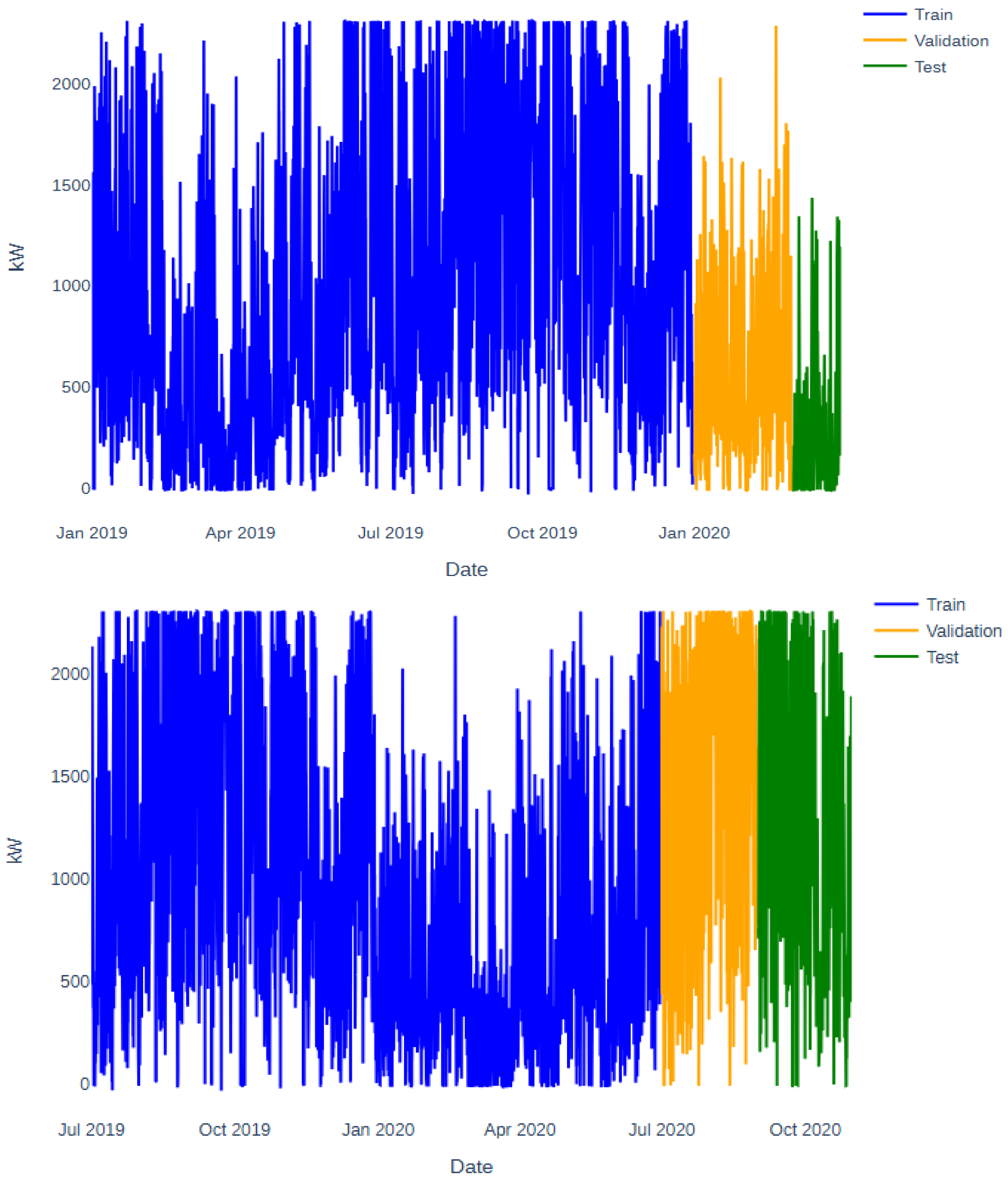
Figure 10 illustrates the wind power output of the wind turbine under study for the two proposed scenarios (A and B). The top image corresponds to Scenario A, while the bottom image corresponds to Scenario B. These are real data from a wind turbine currently in operation. The highest wind potential was observed between July and December 2019 and between July and October 2020, whereas the lowest occurred between January and April of both years. Therefore, it is evident that the two scenarios capture distinct temporal conditions of the wind farm under study.

3.6. Experimental Analysis

In this study, a search for hyperparameters was carried out for each model, using Optuna (version 3.6.1). The number of trials was set to 100 in this study based on a balance between computational cost and the need for sufficient exploration of the hyperparameter space. This choice aligns with the recommendation in Ref. [59], where 100 trials were used in their example for the optimization of hyperparameters. This number allows a good trade-off between model performance and the time available for experimentation.

All experiments were conducted in PyTorch (version 2.3.0), using a system equipped with an Nvidia RTX A4000, a professional-grade GPU based on the Ampere architecture, featuring 16 GB of VRAM and optimized for high-performance computing tasks.

Table 3. Final Results of Hyperparameter Search for All Evaluated Models (Scenario A).

	Parameter	MLP	LSTM	DLinear	T2V-MLP	T2V-LSTM	T2V-DLinear
	seq len	104	52	46	82	46	65
	layers	3	2	-	2	1	-
	hidden layers	(44,206,234)	98	-	(24,684)	149	-
	bidirectional	-	True	-	-	True	-
	epochs	50	50	50	50	50	50
	optimizer	Adam	Adam	Adam	Adam	Adam	Adam
	activation	ReLU	ReLU	-	ReLU	ReLU	-
	dropout	0.1	0.1	-	0.1	0.1	-
	function	-	-	-	cos	sin	sin
	time	35 s	32 s	1 min 2 s	41 s	39 s	1 min 13 s
Parameter	Transformer	Informer	Flowformer	Flashformer	T2V- Transformer	T2V- Informer	T2V- Flowformer	T2V- Flashformer
seq len	53	52	58	93	32	30	49	63
encoder layers	3	2	2	2	1	2	2	2
decoder layers	1	1	2	3	1	2	3	1
epochs	10	10	10	10	10	10	10	10
optimizer	RMSprop	RMSprop	RMSprop	RMSprop	RMSprop	RMSprop	RMSprop	RMSprop
activation	ReLU	ReLU	ReLU	ReLU	ReLU	ReLU	ReLU	ReLU
dropout	0.1	0.1	0.1	0.1	0.1	0.1	0.1	0.1
dmodel	128	64	128	32	64	32	32	256
heads	2	2	8	2	4	2	4	6
dff	768	128	768	64	128	192	96	512
function	-	-	-	-	sin	sin	cos	sin
time	2 min 30 s	2 min 10 s	2 min 14 s	1 min 38 s	2 min 46 s	2 min 25 s	2 min 27 s	1 min 59 s

and

Table 4. Final Results of Hyperparameter Search for All Evaluated Models (Scenario B).

	Parameter	MLP	LSTM	DLinear	T2V-MLP	T2V-LSTM	T2V-DLinear
	seq len	92	77	76	60	74	104
	layers	1	1	-	1	2	-
	hidden layers	246	144	-	197	148	-
	bidirectional	-	True	-	-	True	-
	epochs	50	50	50	50	50	50
	optimizer	Adam	Adam	Adam	Adam	Adam	Adam
	activation	ReLU	ReLU	-	ReLU	ReLU	-
	dropout	0.1	0.1	-	0.1	0.1	-
	function	-	-	-	cos	sin	cos
	time	37 s	35 s	1 min 5 s	42 s	42 s	1 min 16 s
Parameter	Transformer	Informer	Flowformer	Flashformer	T2V- Transformer	T2V- Informer	T2V- Flowformer	T2V- Flashformer
seq len	76	72	55	53	44	30	120	105
encoder layers	3	1	2	1	1	3	2	3
decoder layers	2	2	2	1	1	1	2	1
epochs	10	10	10	10	10	10	10	10
optimizer	RMSprop	Adam	RMSprop	Adam	Adam	SGD	Adam	Adam
activation	ReLU	ReLU	ReLU	ReLU	ReLU	ReLU	ReLU	ReLU
dropout	0.1	0.1	0.1	0.1	0.1	0.1	0.1	0.1
dmodel	256	512	64	64	64	256	128	256
heads	6	2	8	8	6	8	2	8
dff	1536	2048	192	192	384	768	512	1536
function	-	-	-	-	cos	sin	sin	sin
time	2 min 40 s	2 min 30 s	2 min 26 s	1 min 52 s	2 min 58 s	2 min 42 s	2 min 40 s	2 min 10 s

show the final parameters of each model, referencing the best configurations found for Scenario A and Scenario B.

The number of epochs for each model was set based on previous experimentation and the results of hyperparameter optimization. For MLP, LSTM, DLinear, T2V-MLP, T2V-LSTM, and T2V-DLinear models, 50 epochs were selected, as these models generally require more iterations to learn from the data, according to prior experiments. For Transformer, Informer, Flowformer, Flashformer, and the proposed models, the number of epochs was set to 10, as these models typically converge more quickly due to their efficient attention mechanisms. For all models in this study, we developed 16 for batch size. In this study, the sequence length (seq len) was included in the hyperparameter search with values ranging from 6 to 120. This range was selected to ensure the model could learn both short- and long-term dependencies in the time series, which is crucial for accurate forecasting over the 12-h horizon. A shorter seq len might not capture long-term patterns, while a longer one might lead to unnecessary complexity. The label length, set as half of the sequence length, was used consistently across all scenarios to maintain a balanced ratio between input and output. The forecast horizons considered—6, 10, and 12 h—align with the study’s focus on short-term power forecasting, allowing the models to focus on the near-future dynamics of wind power generation.

3.6.1. Scenario A

According to Table 3, Different architectures handle historical data in unique ways, and the sequence length varies based on each model’s ability to process and extract relevant information. The MLP has the largest seq len, with a value of 104, while the T2V-Informer has the smallest, with a seq len of 30. Regarding the number of layers, the MLP has 3, and the T2V-MLP has 2. For the LSTM and the T2V-LSTM, the number of layers is 2 and 1, respectively. Both models are bidirectional, meaning they process the sequence in two directions: from past to future and from future to past. This bidirectionality enables the models to capture global temporal dependencies, leveraging past and future information, which is essential for predicting complex patterns, such as in wind power forecasting. In relation to X-formers and the proposed models, Transformer, Informer and T2V-Flashformer have a greater number of layers in the encoder (3, 2 and 2, respectively) than in the decoder (1, 1 and 1, respectively). For both the T2V-Flowformer and the Flashformer, the encoder consisted of 2 layers, while the decoder had 3 layers. For the T2V-Transformer, T2V-Informer and the Flowformer, the number of layers was the same for encoder and decoder. For all benchmark models, Adam was the best optimizer. For the X-formers and the proposed models, RMSprop was the best optimizer. The activation function resulted in ReLU for all models, and the technique to avoid overfitting (dropout) was set to 0.1 for all models. The higher $d_{model}$ for the models was 256 for the T2V-Flashformer, and the smaller was 32, for T2V-Informer, T2V-Flowformer and the Flashformer. The higher $d_{ff}$ was 768 for Transformer and Flowformer. The smallest was 64 for Flashformer. The higher number of heads was 8 for Flowformer. The higher these three parameters are, the greater the computational cost. Conversely, lower values reduce the demand for computational resources.

3.6.2. Scenario B

According to Table 4, the model with the largest seq len was the T2V-Flowformer, followed by the T2V-Flashformer. This means that the models needed more historical data to make predictions for Scenario B. The number of layers was 1 for both MLP and T2V-MLP. For LSTM and T2V-LSTM, the number of layers was 1 and 2, respectively. Both models are bidirectional, as in Scenario A. The number of encoder layers was greater than that of decoder layers for Transformer, T2V-Informer and T2V-Flashformer architectures. In contrast, for the Informer, the encoder consists of 1 layer, while the decoder comprises 2 layers. For the other models, the number of layers for the encoder and decoder was the same. The models with the highest complexity were the Informer and T2V-Flashformer, with $d_{model}$, heads, and $d_{ff}$ equal to (512, 2, 2048) and (256, 8, 1536), respectively. It was followed by the Transformer, with $d_{model}$, heads, and $d_{ff}$ equal to 256, 6, 1536, respectively. The Adam optimizer was applied to most models, while SGD was applied to T2V-Informer, and RMSprop was applied to the Transformer and Flowformer. The variation in the parameters presented in Table 3 and Table 4 can be explained by the fact that they correspond to two different scenarios, each considering distinct temporal conditions.

3.6.3. Computational Performance and Feasibility Across Both Scenarios

As mentioned before, a total of 100 trials were conducted for each model in the hyperparameter search using Optuna. Table 3 and Table 4 also present the time required for a single trial of each model, considering the total duration (including both training and inference). It is important to note that these times correspond to the best possible configuration obtained from Optuna’s hyperparameter search. These values indicate that the models are computationally feasible and suitable for 12-h-ahead forecasting. Once the best hyperparameters have been determined, they can be directly applied in future forecasts, eliminating the need for additional trials and significantly reducing computational costs. T2V-Transformer had the longest trial time, taking 2 min and 58 s in Scenario B, and 2 min and 46 s in Scenario A. The Transformer followed, with 2 min and 40 s in Scenario B, and 2 min and 30 s in Scenario A, as shown in the tables. This can be attributed to the quadratic complexity of the FullAttention mechanism, as explained in Section 2.4. The results indicate that models employing the ProbSparse Attention, FlowAttention and FlashAttention mechanisms achieved shorter trial times compared to the standard Transformer architecture, which relies on the FullAttention mechanism.

In Scenario A, the T2V-Informer and Informer required approximately 2 min and 25 s and 2 min and 10 s, respectively. The T2V-Flowformer and Flowformer required approximately 2 min and 27 s and 2 min and 14 s, respectively. The T2V-Flashformer and Flashformer completed in 1 min and 59 s and 1 min and 38 s, respectively.

In Scenario B, the T2V-Informer and Informer required approximately 2 min and 42 s and 2 min and seconds. The T2V-Flowformer and Flowformer took approximately 2 min and 40 s and 2 min and 26 s, while the T2V-Flashformer and Flashformer completed in 2 min and 10 s and 1 min and 52 s, respectively.

These results suggest a modest computational efficiency advantage for models using ProbSparse Attention, FlowAttention and FlashAttention over those using FullAttention. In contrast, LSTM and MLP had the shortest trial times, taking 32 and 35 s in Scenario A, and 35 and 37 s in Scenario B, respectively.

4. Results and Discussion

The metrics used to evaluate the performance of the models were Mean Absolute Error (MAE), Root Mean Square Error (RMSE), Improvement over Reference MAE (IoR-MAE), and Improvement over Reference RMSE (IoR-RMSE). The MAE (Equation (8)) measures the average magnitude of the errors between the predicted (${\widehat{y}}_i)$ and observed ($y_i)$ values, while the RMSE (Equation (9)) penalizes larger deviations more heavily by squaring the residuals. The IoR-MAE (Equation (10)) and IoR-RMSE (Equation (11)) express the relative improvement of the evaluated model compared to a reference baseline, the Persistence model.

$$MAE={\displaystyle \frac{1}{n}}{{\displaystyle \sum }}_{i=1}^n\left|y_i-{\widehat{y}}_i\right|$$

(8)

$$RMSE=\sqrt{{\displaystyle \frac{1}{n}}{{\displaystyle \sum }}_{i=1}^n{\left(y_i-{\widehat{y}}_i\right)}^2}$$

(9)

$$IoR\text{-}MAE=\left(1-{\displaystyle \frac{MA{E}_{model}}{MA{E}_{reference}}}\right)·100\%$$

(10)

$$IoR\text{-}RMSE=\left(1-{\displaystyle \frac{RMS{E}_{model}}{RMS{E}_{reference}}}\right)·100\%$$

(11)

where n is the total number of samples. The reference MAE and RMSE correspond to the metrics obtained from the Persistence model. Hence, higher values of IoR-MAE and IoR-RMSE, along with lower MAE and RMSE, indicate better model performance.

According to

Table 5. Comparison of model performance for different forecast horizons (Scenario A).

Model	MAE/IoR-MAE (%)
	6 h		10 h		12 h
Persistence	243.463	0	273.198	0	279.828	0
MLP	222.349	8.67	245.996	9.95	254.032	9.22
T2V-MLP	222.947	8.42	241.690	11.53	249.697	10.76
LSTM	225.592	7.34	248.002	9.22	250.645	10.43
T2V-LSTM	218.730	10.16	249.981	8.49	252.356	9.82
DLinear	218.137	10.40	239.555	12.31	250.375	10.52
T2V-DLinear	213.386	12.35	257.894	5.60	246.195	12.02
Transformer	224.325	7.86	244.365	10.55	254.115	9.18
T2V-Transformer	214.096	12.06	233.430	14.56	241.911	13.55
Informer	217.375	10.71	234.978	13.98	243.698	12.91
T2V-Informer	217.392	10.70	236.326	13.49	241.300	13.76
Flowformer	223.979	8.00	244.266	10.59	249.242	10.93
T2V-Flowformer	219.680	9.77	238.644	12.65	247.056	11.71
Flashformer	215.573	11.45	235.273	13.88	246.213	12.01
T2V-Flashformer	214.368	11.95	235.402	13.83	242.598	13.30
Model	RMSE/IoR-RMSE (%)
	6 h		10 h		12 h
Persistence	342.520	0	378.050	0	384.270	0
MLP	294.207	14.10	318.141	15.84	326.291	15.08
T2V-MLP	297.990	12.99	324.162	14.25	330.686	13.94
LSTM	299.486	12.56	325.241	13.96	331.262	13.79
T2V-LSTM	293.626	14.27	320.027	15.35	326.267	15.09
DLinear	297.971	13.00	321.293	15.01	328.022	14.64
T2V-DLinear	298.052	12.98	327.494	13.37	324.737	15.49
Transformer	297.550	13.13	322.429	14.71	330.681	13.94
T2V-Transformer	287.613	16.03	310.545	17.85	316.146	17.73
Informer	297.873	13.03	320.820	15.14	324.750	15.48
T2V-Informer	294.250	14.09	313.287	17.13	316.640	17.59
Flowformer	298.385	12.88	322.098	14.80	326.549	15.02
T2V-Flowformer	296.478	13.44	320.958	15.10	327.351	14.81
Flashformer	295.377	13.76	321.323	15.00	329.660	14.21
T2V-Flashformer	291.201	14.98	315.353	16.58	320.213	16.67

, the T2V-DLinear model achieved the best performance for the MAE and IoR-MAE metrics at the 6-h horizon, with values of 213.386 and 12.35%, respectively, followed by T2V-Transformer, which recorded an MAE of 214.096 and an IoR-MAE of 12.06%. At the 10-h horizon, T2V-Transformer outperformed all models with an IoR-MAE of 14.56%, Subsequently, Flashformer and T2V-Flashformer achieved IoR- MAE values of 13.88% and 13.83%, respectively. For the 12-h horizon, the best results were achieved by T2V-Informer, T2V-Transformer and T2V-Flashformer, with IoR-MAE values of 13.76%, 13.55% and 13.30%, respectively. The MLP, LSTM, and DLinear models presented lower performance, with IoR-MAE values of 9.22%, 10.43%, and 10.52%, respectively. Overall, T2V-Transformer demonstrated the greatest consistency and best performance across all horizons for both MAE and IoR-MAE metrics, followed by the T2V-Flashformer. Regarding RMSE and IoR-RMSE metrics, the T2V-Transformer and T2V-Flashformer models demonstrated superior performance. At the 6-h horizon, T2V-Transformer was the only model to surpass an IoR-RMSE of 16%, reaching 16.03%. T2V-Flashformer, in turn, achieved an IoR-RMSE of approximately 14.98%. At the 10-h horizon, the IoR-RMSE values were 17.85% for T2V-Transformer, 17.13% for T2V-Informer and 16.58% for T2V-Flashformer, while for the 12-h horizon, the IoR-RMSE values were 17.73% for T2V-Transformer, 17.59% for T2V-Informer and 16.67% for T2V-Flashformer. The MLP, LSTM, and DLinear models demonstrated inferior performance, achieving 15.08%, 13.79%, and 14.64%, respectively, for the same metric and forecast horizon. In general, T2V-Transformer exhibited the best performance for all horizons, followed by T2V-Informer and T2V-Flashformer for the RMSE and IoR-RMSE metrics. Analyzing the horizons and evaluation metrics presented in Table 5, the T2V-Transformer, T2V-Informer and T2V-Flashformer models demonstrated consistency and reliability, making them the most suitable choices for power prediction under this approach. While T2V-DLinear achieved the best performance for MAE and IoR-MAE at the 6-h horizon, its performance was inconsistent across other horizons and less competitive for RMSE and IoR-RMSE metrics. Consequently, T2V-DLinear is not as suitable for Scenario A, compared to the T2V-Flashformer, T2V-Informer and T2V-Transformer models.

According to

Table 6. Comparison of model performance for different forecast horizons (Scenario B).

Model	MAE/IoR-MAE (%)
	6 h		10 h		12 h
Persistence	472.842	0	534.238	0	539.987	0
MLP	401.633	15.05	422.769	20.86	428.720	20.60
T2V-MLP	399.556	15.06	421.157	21.16	425.582	21.18
LSTM	404.243	14.50	430.225	19.46	436.876	19.09
T2V-LSTM	406.040	14.12	430.061	19.50	427.028	20.91
DLinear	400.527	15.29	423.949	20.64	427.896	20.75
T2V-DLinear	404.430	14.46	427.453	20.54	427.903	20.75
Transformer	402.317	14.91	427.499	19.90	433.263	19.76
T2V-Transformer	397.342	15.97	425.233	20.40	431.457	20.09
Informer	403.851	14.59	424.184	20.60	437.251	19.02
T2V-Informer	386.323	18.29	410.521	23.16	419.677	22.28
Flowformer	405.141	14.32	425.564	20.34	429.519	20.46
T2V-Flowformer	387.832	17.98	407.396	23.74	407.848	24.47
Flashformer	392.619	16.96	422.642	20.89	427.476	20.83
T2V-Flashformer	386.651	18.23	406.608	23.89	408.364	24.37
Model	RMSE/IoR-RMSE (%)
	6 h		10 h		12 h
Persistence	610,223	0	674.159	0	676.469	0
MLP	492,236	19.33	514.570	23.67	519.293	23.25
T2V-MLP	496,024	18.71	513.812	23.78	514.389	23.95
LSTM	488,402	19.96	514.152	23.73	519.833	23.15
T2V-LSTM	497,665	18.44	521.738	22.60	516.666	23.62
DLinear	496.257	18.67	516.697	23.35	520.411	23.06
T2V-DLinear	496.896	18.57	514.842	23.63	517.046	23.56
Transformer	492.053	19.36	515.418	23.54	519.182	23.25
T2V-Transformer	484.898	20.54	512.338	24.00	519.001	23.28
Informer	486.768	20.23	509.272	24.46	518.525	23.35
T2V-Informer	469.356	23.08	493.266	26.83	502.084	25.78
Flowformer	492.491	19.29	512.717	23.95	511.864	24.33
T2V-Flowformer	472.943	22.49	487.814	27.64	488.135	27.84
Flashformer	481.754	21.05	511.446	24.13	514.838	23.89
T2V-Flashformer	470.586	22.88	489.812	27.34	490.786	27.45

, the T2V-Flashformer and T2V-Flowformer models consistently achieved the best performance in virtually all forecasting horizons and evaluation metrics. For the MAE and IoR-MAE metrics, T2V-Flashformer yielded the best results, with IoR-MAE values of 18.23% for the 6-h horizon and 23.89% for the 10-h horizon, while T2V-Flowformer followed closely with 17.98% and 23.74% for the same horizons, respectively. At the 12-h horizon, T2V-Flowformer and T2V-Flashformer recorded IoR-MAE values of 24.47% and 24.37%, respectively. Notably, these two models were the only ones to exceed 23% IoR-MAE at the 10-h horizon and 24% at the 12-h horizon. At the 12-h forecasting horizon, the MLP, LSTM, and DLinear models achieved IoR-MAE values of 20.60%, 19.09%, and 20.75%, respectively. For the RMSE and IoR-RMSE metrics, T2V-Informer achieved the best performance at the 6-h horizon, with an IoR-RMSE of 23.08%, followed by T2V- Flashformer with 22.88% and T2V-Flowformer with 22.49%. For the 10- and 12-h horizons, T2V-Flowformer outperformed all other models, recording IoR-RMSE values of 27.64% and 27.84%, respectively, while T2V-Flashformer obtained 27.34% and 27.45% for the same horizons. The MLP, LSTM, and DLinear models performed worse, with values of 23.67%, 23.73%, and 23.35% at the 10-h horizon, and 23.23%, 23.15%, and 23.06% at the 12-h horizon, respectively. As shown in Table 6, both T2V-Flowformer and T2V-Flashformer proved to be the most suitable models for Scenario B.

According to Figure 10, in Scenario B, the test period exhibits higher wind power values, with more frequent and intense peaks. This indicates greater variability and magnitude in the data to be forecasted, increasing the complexity of the forecasting task. Consequently, the models show higher MAE and RMSE values in this scenario compared to Scenario A. However, as shown in Table 5 and Table 6, the IoR-MAE and IoR-RMSE values for the models evaluated in this study are consistently higher in Scenario B. This suggests that, despite the increase in absolute errors due to the more challenging test conditions, the proposed models outperform the Persistence model by a larger margin. Therefore, the higher IoR metrics in Scenario B highlight the robustness and effectiveness of the models under more demanding forecasting conditions.

To verify the reliability of the performance gains reported in Table 5 and Table 6, paired t-tests and Wilcoxon signed-rank tests (p < 0.05) were conducted on the IoR-RMSE values for the 12-h forecast horizon. The tests were performed at a 5% significance level to assess whether the improvements over the persistence model were statistically significant. The results, presented in

Table 7. Statistical significance tests for the IoR-RMSE metric under Scenarios A and B. The paired t-test and Wilcoxon signed-rank test were applied to assess whether the proposed models achieved statistically significant improvements over the persistence baseline.

Model	Scenario A		Scenario B
	p (t-Test)	p (Wilcoxon)	p (t-Test)	p (Wilcoxon)
MLP	0.001	0.001	<0.001	<0.001
T2V-MLP	<0.001	<0.001	<0.001	<0.001
LSTM	<0.001	<0.001	<0.001	<0.001
T2V-LSTM	<0.001	<0.001	<0.001	<0.001
DLinear	<0.001	<0.001	<0.001	<0.001
T2V-DLinear	<0.001	<0.001	<0.001	<0.001
Transformer	0.001	0.001	0.008	0.008
T2V-Transformer	<0.001	<0.001	0.001	0.001
Informer	0.001	0.001	<0.001	<0.001
T2V-Informer	0.010	0.010	<0.001	<0.001
Flowformer	0.001	0.001	0.001	0.001
T2V-Flowformer	0.001	0.001	0.026	0.026
Flashformer	0.001	0.001	0.001	0.001
T2V-Flashformer	0.001	0.001	0.021	0.021

, indicate that all proposed models exhibited statistically significant differences compared with the baseline across Scenario A and Scenario B. In most cases, p-values were below 0.001 for both tests, confirming the robustness of the observed improvements. These findings demonstrate that the reported IoR-RMSE gains are not due to random variation but reflect consistent performance advantages of the models employed in this study.

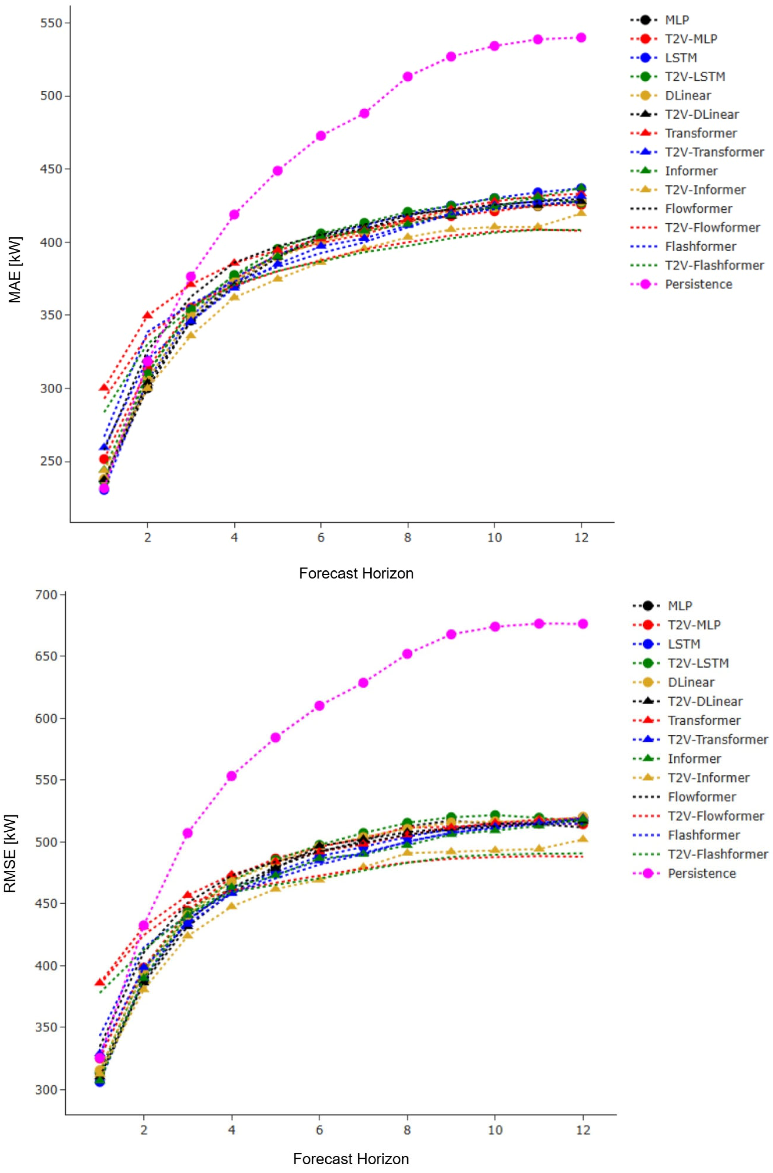
Figure 11 and Figure 12 depict the performance of the models across different forecast horizons, offering a comprehensive and clear visualization of the MAE and RMSE metrics. According to Figure 11, for Scenario A, it is evident that the proposed models (specifically T2V-Transformer, T2V-Informer and T2V-Flashformer) outperformed the benchmark models, particularly in the later horizons. This trend is even more pronounced in RMSE, where the T2V-Transformer and T2V-Flashformer consistently demonstrated superior performance across nearly all forecast horizons, with the performance gap becoming increasingly significant beyond the 4-h horizon. According to Figure 12, for Scenario B, the proposed models—specifically T2V-Flowformer and T2V-Flashformer—significantly begin to outperform the baseline models after the 4-h horizon. This reflects a progressive enhancement in forecasting performance as the prediction horizon increases. Although in the very short term (e.g., horizon 1) their performance may initially fall behind that of simpler benchmarks, this behavior is likely attributable to their reliance on temporal encoding via Time2Vec and complex attention mechanisms, which are more effective at capturing latent temporal dependencies over slightly longer horizons. From horizon three onward, however, both models exhibit a marked reduction in forecast error and consistently outperform all baseline models up to the 12-h horizon. These findings suggest that the proposed architectures are particularly well-suited to short-term forecasting tasks involving multi-hour horizons, such as those analyzed in this study (i.e., 6, 10, and 12 h).

Analyzing all models without the addition of Time2Vec, it was observed that, for Scenario A, Flashformer demonstrated the best performance in terms of the MAE metric across all horizons. For the RMSE metric, the best-performing model at the 6-, 10-, and 12-h horizons was the MLP. Flashformer, DLinear, and Flowformer were the second-best performers at the 6-, 10-, and 12-h horizons, respectively, with Flashformer also closely trailing DLinear at the 10-h mark. In Scenario B, Flashformer outperformed other models for the MAE metric at the 6-, 10-, and 12-h horizons. For the same metric, DLinear was the second-best performer at the 6- an12-hourur horizons, while MLP ranked second at 10 h. Regarding the RMSE metric, Flashformer achieved the best performance at the 6- and 10-h horizons, whereas Flowformer was the top performer at 12 h.

4.1. Impact of Time2Vec Integration on Models’ Performance

In general, the addition of Time2Vec improved the performance of the models, as shown in

Table 8. Improvements with addition of Time2Vec for Scenario A.

	MAE			RMSE
Model	6 h	10 h	12 h	6 h	10 h	12 h
MLP	222.349	245.996	254.032	294.207	318.141	326.291
T2V-MLP	222.947	241.690	249.697	297.990	324.162	330.686
Improvement (%)	−0.27	1.75	1.70	−1.29	−1.89	−1.35
LSTM	225.592	248.002	250.645	299.486	325.241	331.262
T2V-LSTM	218.730	249.981	252.356	293.626	320.027	326.267
Improvement (%)	3.04	−0.80	−0.68	1.96	1.60	1.51
DLinear	218.137	239.555	250.375	297.971	321.293	328.022
T2V-DLinear	213.386	257.894	246.195	298.052	327.494	324.737
Improvement (%)	2.18	−7.66	1.67	−0.03	−1.93	1.00
Transformer	224.325	244.365	254.115	297.550	322.429	330.681
T2V-Transformer	214.096	233.430	241.911	287.613	310.545	316.146
Improvement (%)	4.56	4.47	4.80	3.34	3.69	4.40
Informer	217.375	234.978	243.698	297.873	320.820	324.750
T2V-Informer	217.392	236.326	241.300	294.250	313.287	316.640
Improvement (%)	−0.01	−0.57	0.98	1.22	2.35	2.50
Flowformer	223.979	244.266	249.242	298.385	322.098	326.549
T2V-Flowformer	219.680	238.644	247.056	296.478	320.958	327.351
Improvement (%)	1.92	2.30	0.88	0.64	0.35	−0.25
Flashformer	215.573	235.273	246.213	295.377	321.323	329.660
T2V-Flashformer	214.368	235.402	242.598	291.201	315.353	320.213
Improvement (%)	0.56	−0.05	1.47	1.41	1.86	2.87

and

Table 9. Improvements with addition of Time2Vec for Scenario B.

	MAE			RMSE
Model	6 h	10 h	12 h	6 h	10 h	12 h
MLP	401.633	422.769	428.720	492.236	514.570	519.293
T2V-MLP	399.556	421.157	425.582	496.024	513.812	514.389
Improvement (%)	0.52	0.38	0.73	−0.77	0.15	0.94
LSTM	404.243	430.225	436.876	488.402	514.152	519.833
T2V-LSTM	406.040	430.061	427.028	497.665	521.738	516.666
Improvement (%)	−0.44	0.04	2.25	−1.90	−1.48	0.61
DLinear	400.527	423.949	427.896	496.257	516.697	520.411
T2V-DLinear	404.430	427.453	427.903	496.896	514.842	517.046
Improvement (%)	−0.97	−0.83	−0.01	−0.13	0.36	0.65
Transformer	402.317	427.499	433.263	492.053	515.418	519.182
T2V-Transformer	397.342	425.233	431.457	484.898	512.338	519.001
Improvement (%)	1.24	0.53	0.42	1.45	0.60	0.03
Informer	403.851	424.184	437.251	486.768	509.272	518.525
T2V-Informer	386.323	410.521	419.677	469.356	493.266	502.084
Improvement (%)	4.34	3.22	4.02	3.58	3.14	3.17
Flowformer	405.141	425.564	429.519	492.491	512.717	511.864
T2V-Flowformer	387.832	407.396	407.848	472.943	487.814	488.135
Improvement (%)	4.27	4.27	5.05	3.97	4.86	4.64
Flashformer	392.619	422.642	427.476	481.754	511.446	514.838
T2V-Flashformer	386.651	406.608	408.364	470.586	489.812	490.786
Improvement (%)	1.52	3.79	4.47	2.32	4.23	4.67

for Scenarios A and B, respectively. Values are expressed as percentages, with negative numbers indicating that the addition of Time2Vec did not improve the models.

According to Table 8, for Scenario A, improvements were observed across nearly all horizons and metrics of the X-formers. Notably, the T2V-Transformer demonstrated significant gains at the 6-, 10-, and 12-h horizons, achieving a 4.56%, 4.47% and 4.80% improvement over the Transformer in MAE, and 3.34%, 3.69% and 4.40% in RMSE, respectively. The T2V-Informer outperformed the Informer in terms of the RMSE metric, with improvements of 1.22%, 2.35% and 2.50% for the 6-, 10-, and 12-h forecast horizons, respectively. For the MAE metric, the results were nearly identical for the 6- and 10-h horizons, while a slight improvement was observed for the 12-h horizon. The T2V-Flowformer outperformed the Flowformer, with an improvement of 1.92%, 2.30%, and 0.88% in MAE on the 6-, 10-, and 12-h horizons. The T2V-Flashformer showed consistent improvements across all horizons and metrics, with 2.87% enhancement in RMSE at the 12-h horizon compared to the Flashformer. In comparison to the benchmark models, the gains were less pronounced. However, some improvements were observed in specific horizons and metrics. For instance, T2V-MLP outperformed MLP at the 10- and 12-h horizons in MAE metric, with improvements of 1.75% and 1.70%, respectively. Conversely, for the RMSE metric, MLP consistently outperformed T2V-MLP across all horizons. T2V-LSTM showed better performance than LSTM for all horizons in the RMSE metric. Similarly, T2V-DLinear outperformed DLinear on the 12-h horizon in both MAE and RMSE metrics.

According to Table 9, for Scenario B, the addition of Time2Vec improved all X-formers. The T2V-Flashformer showed consistent improvements over the Flashformer in all metrics and horizons, particularly in the MAE metric, with gains of 3.79% and 4.47% at the 10- and 12-h horizons, respectively. For the RMSE metric, the improvements were 2.32%, 4.23% and 4.67% on the 6, 10- and 12-h horizons, respectively. Compared to the Informer, T2V-Informer achieved improvements of 4.34%, 3.22%, and 4.02% at the 6-, 10-, and 12-h horizons for MAE, and 3.58%, 3.14%, and 3.17% for RMSE. Similarly, the T2V-Flowformer consistently outperformed the baseline Flowformer across all evaluation metrics and forecasting horizons. At the 6-, 10-, and 12-h horizons, it achieved notable improvements, with reductions in MAE of 4.27%, 4.27%, and 5.05%, and in RMSE of 3.97%, 4.86%, and 4.96%, respectively. For the benchmark models, improvements with the inclusion of Time2Vec were less pronounced, but still present. The T2V-MLP consistently outperformed the standard MLP in terms of MAE across all forecasting horizons, and also in RMSE, except at the 6-h horizon. The T2V-LSTM showed a notable improvement over the LSTM at the 12-h horizon for the MAE metric (2.25%). In contrast, the integration of Time2Vec into the DLinear model did not lead to significant gains.

According to Table 8 and Table 9, all models were trained and optimized through an extensive hyperparameter search procedure comprising 100 independent trials per model, as described in Section 3.6. This process ensured that the reported results correspond to the best-performing configuration of each model, enabling a fair and reliable comparison between the baseline architectures and their Time2Vec-enhanced counterparts. Therefore, the observed differences can be attributed to the intrinsic characteristics of the temporal encoding strategies rather than to suboptimal hyperparameter configurations.

4.2. Comparative Analysis of Model Performance, Computational Cost, and Scalability

Table 10. Comparative evaluation criteria of the models used in this study.

Models	Sensitivity to Temporal Patterns	Feature Extraction Type	Scalability for Large Datasets	GPU Total Experiment Time (100 Trials)		Computational Cost
				Scenario A	Scenario B	Scenario A	Scenario B
MLP	Low	Manual feature engineering	Low	58 min	1 h 1 min	Low	Low
T2V-MLP	Moderate	Manual feature engineering	Low	1 h 8 min	1 h 10 min	Low	Low
LSTM	Moderate	Implicit learning of patterns	Moderate	53 min	58 min	Low	Low
T2V-LSTM	High	Implicit learning of patterns	Moderate	1 h 5 min	1 h 10 min	Low	Low
DLinear	Moderate	Linear modeling with decomposition	High	1 h 43 min	1 h 48 min	Low	Low
T2V-DLinear	High	Linear modeling with decomposition	High	2 h 1 min	2 h 6 min	Moderate	Moderate
Transformer	High	Learning based on FullAttention	Moderate	4 h 10 min	4 h 26 min	High	High
T2V- Transformer	Very High	Learning based on FullAttention	Moderate	4 h 36 min	4 h 56 min	High	High
Informer	High	Learning based on ProbSparse Attention	Very High	3 h 48 min	3 h 58 min	High	High
T2V-Informer	Very High	Learning based on ProbSparse Attention	Very High	4 h 2 min	4 h 20 min	High	High
Flowformer	High	Learning based on FlowAttention	Very High	3 h 43 min	4 h 3 min	High	High
T2V-Flowformer	Very High	Learning based on FlowAttention	Very High	4 h 5 min	4 h 26 min	High	High
Flashformer	High	Learning based on FlashAttention	Very High	2 h 43 min	3 h 6 min	Moderate	High
T2V- Flashformer	Very High	Learning based on FlashAttention	Very High	3 h 18 min	3 h 36 min	High	High

presents a comparative evaluation of the prediction models used in this study. The models vary in their sensitivity to temporal patterns, with X-formers generally exhibiting a high capacity for capturing such dependencies. The addition of Time2Vec further enhances this sensitivity, as it explicitly encodes temporal information. This effect was observed not only in the proposed models but also when Time2Vec was integrated into MLP, LSTM, and DLinear, leading to improved temporal pattern recognition. In this study, the time series data is directly fed into each model. While MLP lacks inherent temporal memory, LSTM and Transformer capture dependencies through their sequential architectures—LSTM via its internal memory and Transformer through self-attention mechanisms, which dynamically focus on relevant time steps. X-formers leverage their respective attention mechanisms for temporal representation learning, while DLinear employs a decomposition technique that aids in time series modeling.

Regarding computational performance, the total experiment time for each model—comprising training over 100 trials and inference (prediction generation)—was measured using the GPU employed in this study. As shown in Table 8, T2V-Transformer had the longest experiment time, approximately 4 h and 36 min for Scenario A and 4 h and 56 min for Scenario B. Comparing attention mechanisms, ProbSparse Attention, FlowAttention and FlashAttention exhibit lower computational costs than FullAttention, demonstrating significant advantages in both Scenario A and Scenario B. LSTM had the shortest experiment time, around 58 min for Scenario A and 1 h and 1 min for Scenario B. It can be observed that Scenario B required slightly more time for all models. This can be attributed to the differences in the temporal behavior of the series and the hyperparameter settings used. Models and data with more complex temporal patterns typically require more processing and training time.

Furthermore, the inclusion of Time2Vec in the models’ architecture increased the total duration of the experiments, due to the additional computation required to capture specific temporal patterns. The computational cost of each model was evaluated based on the total duration of the experiment. Models with execution times below 2 h were classified as having low computational cost, those above 2 h and below 3 were classified as having moderate cost. And above 3 h as having high cost. Finally, regarding scalability for large datasets, MLP has low scalability due to its inability to capture temporal dependencies effectively. LSTM has moderate scalability, as it processes long sequences sequentially, which can become a bottleneck for large datasets. DLinear, benefiting from its linear decomposition approach, achieves high scalability. Transformer has moderate scalability, as its quadratic complexity can limit its efficiency for very long sequences. In contrast, Informer, Flowformer and Flashformer exhibit very high scalability, as their specialized attention mechanisms are optimized for long time series sequences, significantly improving computational efficiency.

Despite differences in computational cost and scalability, all evaluated models are viable for short-term operational wind power forecasts with a 12-h forecast horizon. The experiment times reported in this subsection correspond to 100 trials; the time required to generate a single forecast is substantially shorter (see Table 3 and Table 4), further confirming the practical applicability of all models for 12-h forecasts.

The results presented in this section demonstrate that Transformer-based models—particularly those enhanced with Time2Vec—are highly effective for wind power forecasting, consistently outperforming established models in the literature across multiple forecast horizons. In Scenario A, the T2V-Transformer and T2V-Flashformer models outperformed all reference models (MLP, LSTM, DLinear, T2V-MLP, T2V-LSTM and T2V-DLinear) in virtually all metrics and horizons evaluated. In Scenario B, the T2V-Informer, T2V-Flowformer and T2V-Flashformer models similarly outperformed the reference models, confirming their robustness and predictive accuracy, as discussed throughout this paper.

5. Conclusions

In this study, we propose four new models for short-term wind power forecasting, applied to operational wind turbines located in the Northeast of Brazil. To ensure a robust forecast analysis and evaluate the models’ performance under variable temporal conditions, two scenarios were considered: Scenario A, with a test period spanning from summer to autumn, and Scenario B, covering the transition from winter to spring.

The proposed models integrate the Time2Vec layer to enhance the representation of temporal patterns in the data. A sensitivity analysis was performed with three arrangements, identifying the configuration that optimized model performance. The best results were obtained when Time2Vec was applied only at the encoder input (Arrangement I), preserving the decoder’s ability to generate outputs from the encoded representations.

In addition, this study explored alternative attention mechanisms, replacing FullAttention with ProbSparse Attention, FlowAttention and FlashAttention in the Informer, Flowformer and Flashformer models to mitigate the quadratic complexity of traditional attention. This is the first application of the Flashformer model to wind power forecasting, and also the first integration of Time2Vec with multiple attention mechanisms in this context.

The proposed models were benchmarked against MLP, LSTM, and DLinear—each also tested with Time2Vec integration. Overall, the results demonstrate that the proposed approach significantly improves forecasting accuracy and computational efficiency, confirming its effectiveness for short-term wind power prediction.

Based on the proposed methodology and the results presented, we can summarize the main conclusions drawn from this work as follows:

• The framework developed in this study proved highly effective, incorporating preprocessing, data handling, and the use of Optuna for efficient hyperparameter optimization. This approach helped prevent overfitting and identified the best possible model configurations.
• The proposed methodology demonstrated its effectiveness in predicting wind turbine power, with the models showing substantial improvements over the Persistence model. The results achieved in this study contribute to advancing the field of wind energy forecasting, offering valuable insights for optimizing predictive models in renewable energy applications.
• The sensitivity analysis of Time2Vec integration into the Transformer architecture facilitated the identification of the optimal configuration for this application. This addition proved particularly advantageous for the X-formers, with the Flowformer and Flashformer models showing improvements in virtually all scenarios.
• In Scenario A, the best-performing models were T2V-Transformer, T2V-Informer and T2V-Flashformer, demonstrating greater consistency across all horizons and metrics. For the 12-h forecasting task, these models achieved IoR-MAE values of 13.55%, 13.76% and 13.30%, respectively, outperforming MLP (9.22%), LSTM (10.43%), and DLinear (10.52%). Similarly, in the IoR-RMSE metric, T2V-Transformer, T2V-Informer and T2V-Flashformer reached 17.73%, 17.59% and 16.67%, while MLP, LSTM, and DLinear obtained 15.08%, 13.79%, and 14.64%, respectively. In Scenario B, the best-performing models were T2V-Flowformer and T2V-Flashformer. For the 12-h horizon, they achieved IoR-MAE values of 24.47% and 24.37%, surpassing MLP (20.60%), LSTM (19.09%), and DLinear (20.75%). In the IoR-RMSE metric, the T2V-Flowformer and T2V-Flashformer reached 27.84% and 27.45%, while MLP, LSTM, and DLinear obtained 23.23%, 23.15%, and 23.06%, respectively.
• The ProbSparse Attention, FlowAttention and FlashAttention mechanisms demonstrated lower computational costs compared to FullAttention, as evidenced by shorter trial times in both scenarios. Regarding predictive performance, the T2V-Transformer showed superior results in Scenario A, except for the MAE and IoR-MAE metrics at the 12-h horizon, where the T2V-Informer performed slightly better. In Scenario B, however, the T2V-Informer, T2V-Flowformer and T2V-Flashformer outperformed the T2V-Transformer, suggesting that these models are better suited for this specific context.
• The proposed models are the most suitable for this study, consistently delivering the best results across all metrics and time horizons. By outperforming the benchmarks in nearly all scenarios, they represent a significant advancement in the state of the art. Their improved predictive accuracy enhances the operational efficiency of wind farms, optimizing maintenance strategies and overall reliability. Additionally, they contribute to a more effective use of renewable resources, such as wind energy.

However, it is important to note that this study was conducted using data from a wind farm located in the Northeast of Brazil. Consequently, the generalization of the proposed models to other geographic regions—particularly those with complex topography, such as mountainous or coastal areas—should be further validated in future studies.

Furthermore, for broader deployment and long-term reliability—particularly in sites with complex or highly variable wind patterns—extended datasets covering longer periods would allow the models to more effectively capture seasonal cycles and rare meteorological events. Future implementations should therefore consider comprehensive data collection and training strategies to further enhance robustness and generalization.

This research presents a robust approach, with an acceptable execution time and feasibility for the proposed models, providing power forecasts 12 h ahead in the time horizon. Based on the adopted methodology, the developed models, and the results achieved, this work can contribute to maximizing the productive efficiency of wind farms worldwide, while also mitigating environmental impacts through the efficient and sustainable use of wind energy. Moreover, by integrating interpretable temporal encodings such as Time2Vec within attention-based architectures, this study helps reduce the “black-box” nature often associated with Transformer-based models, fostering greater confidence and transparency in their practical applications.

6. Future Perspectives

In future perspectives, the models presented in this study are expected to be applied to medium- and long-term wind power forecasting, with further evaluations across different time horizons. Another promising direction involves testing these models on datasets collected from wind farms located in diverse geographic regions and under distinct topographic and climatic conditions. This broader validation would help assess their robustness and generalization in more complex wind regimes, such as those found in mountainous or coastal environments.

Additionally, they may be employed in other wind-related tasks, such as wind speed forecasting and anomaly detection. The integration of ensemble techniques could further enhance forecasting accuracy and robustness by leveraging the strengths of multiple models. The proposed architectures are also adaptable to alternative attention mechanisms, including those currently available and those that may emerge in the near future. Moreover, these models have broad applicability in time series forecasting across diverse domains, such as finance, climate science, economics, and healthcare.