Prediction of Fluid Pressure Dynamics in Deflagration Fracturing for Unconventional Reservoir Stimulation Based on Physics-Guided Graph Neural Network

Abstract

Deflagration fracturing is a gas-dominated, water-free reservoir stimulation technology that has shown strong potential in unconventional, low-permeability, or water-sensitive reservoirs such as coalbed methane and shale gas formations. Accurate prediction of fluid pressure variations, critical for optimizing fracture propagation and stimulation performance, is challenging. While field experiments and numerical simulations offer reliable predictions, they are hindered by high risks, costs, and computational complexity due to multi-physics coupling, Moreover, purely data-driven machine learning methods often exhibit poor generalization and may produce predictions that deviate from fundamental physical principles. To address these challenges, a physics-guided graph neural network (PG-GNN) is proposed in this study to predict the evolution of fluid pressure, the key driving factor governing fracture propagation, from a mechanistic perspective. The proposed method integrates governing equations and physical constraints to construct geometric, physical, and hybrid features and employs a graph neural network encoder to capture the spatial correlations among these features, thereby forming a deep learning framework with strong physical consistency. A multi-task loss function is further employed to balance predictive accuracy and physical rationality. Finally, the proposed model is validated using a high-resolution dataset generated by a CDEM-based numerical simulator, achieving a minimum MAPE of 0.313% and a minimum MSE of 2.309 × 10⁻⁴ on the test dataset, outperforming baseline models in both accuracy and stability and demonstrating strong extrapolation capability.

1. Introduction

Deflagration fracturing, also known as high-energy gas fracturing, has emerged as an alternative stimulation technique for unconventional reservoirs development (e.g., coalbed methane, shale gas) [1,2,3]. Compared with hydraulic fracturing, which requires large fluid volumes and may damage water-sensitive or low-permeability formations, deflagration fracturing generates a rapid gas-phase reaction that produces strong millisecond-scale shock loads and creates near-wellbore radial fractures. These characteristics make it a promising and environmentally compatible alternative in formations where conventional hydraulic techniques are limited.

Accurate prediction of fracture propagation and fluid-pressure evolution is essential for safe and effective design of deflagration treatments. The process is governed by tightly coupled explosive-wave dynamics, transient rock failure, and rapid fluid flow, all evolving on millisecond timescales and with fracture growth largely unobservable in the field [4,5]. In practice, full-scale experiments are difficult to conduct because the rapid gas-phase reaction generates high-energy shock waves that pose operational hazards (e.g., casing deformation, wellbore damage, and wellhead pressure surges) and require specialized high-speed diagnostics that substantially increase testing cost [6,7]. Moreover, the strong multi-physical coupling and millisecond-scale evolution of deflagration fracturing make the resulting fracture network and internal pressure distribution extremely challenging to characterize or predict using conventional approaches.

Current research on modeling deflagration fracturing has relied on field experiments and high-fidelity numerical modeling. Experimental studies have shown that deflagration stimulation produces rapid rock failure and complex near-wellbore fracture networks distinct from those produced by hydraulic fracturing [6,8,9], but full-scale tests remains costly, difficult to instrument at the millisecond scale, and constrained by operational risk. High-fidelity numerical models, particularly those based on the Continuum–Discontinuum Element Method (CDEM), have been used to simulate shock loading, dynamic fracture propagation, and transient fracture–flow interactions with good physical fidelity [1,2,10], but their computational cost limits their use in iterative design. These challenges highlight the need for fast surrogate models capable of predicting fluid-pressure evolution with physical consistency.

Machine learning has been increasingly applied to fracture mechanics and reservoir simulation, achieving strong predictive performance across a range of physical systems [11,12,13,14,15,16,17,18,19]. However, most existing ML models rely on structured spatial discretization, slowly evolving fracture geometries, or controllable hydraulic-driven loading conditions and therefore cannot capture the shock-driven, millisecond-scale, and topologically dynamic fracture evolution characteristic of deflagration fracturing. In unconventional reservoir fracturing applications, current ML applications primarily focus on two categories. The first focuses on surrogate models that learn static mappings from engineering or geological parameters to performance metrics, enabling rapid design optimization for hydraulic or deflagration fracturing treatments [20,21]. The second aims to learn dynamic evolution of flow and fractures using encoder-decoder architectures, primarily for hydraulic fracturing and multiphase flow in complex fractured reservoirs [22,23]. While the former largely ignores transient fracture evolution, the latter is tailored to controllable injection processes and fixed discretization and does not explicitly model pressure fields over an irregular, rapidly changing fracture network driven by explosive loading.

Physics-informed and physics-guided neural network frameworks incorporate governing equations or physical constraints into models by penalizing PDE residuals and boundary condition violations, often on structured grids using fully connected or convolutional architecture [24,25]. Although these approaches provide strong physical consistency, they are difficult to extend to deflagration fracturing, where the fracture geometry evolves rapidly and irregularly under shock loading. Existing GNN-based studies in fracture mechanics primarily address quasi-static or hydraulically driven propagation and assume slowly changing fracture topologies. In contrast, the proposed PG-GNN embeds physics directly on an irregular, dynamically evolving fracture graph through node- and edge-level descriptors derived from the governing fracture-flow equations, enabling pressure prediction under the millisecond-scale, explosively driven conditions unique to deflagration fracturing.

During the deflagration fracturing, the evolution of fluid pressure serves as the key driving force for fracture propagation after the initial shock loading. Pressure gradients determine both the spatial distribution of fracture opening and the transport of gas through newly formed fracture paths. However, modeling fluid pressure dynamics remains highly challenging due to its sensitivity to various coupled factors such as fracture propagation mechanisms and in situ stress conditions. Despite being a pivotal issue in deflagration fracturing, there is currently a lack of machine learning-based models specifically designed to capture the evolution of fluid pressure in this context.

To address this gap, this study focuses on modeling fluid pressure evolution within the fracture network during deflagration fracturing, and proposes a physics-guided graph neural network (PG-GNN) model. The CDEM model is used solely as a high-fidelity simulator to generate physically consistent training data and to provide the governing fracture-flow relationships that guide the construction of physics-based features in the PG-GNN framework. The proposed method represents the reservoir as a graph capturing the spatial connectivity of fracture elements, encodes geometric and flow-related descriptors on nodes and edges, and incorporates physics guidance through composite features and constraints. By leveraging the inductive biases of message-passing GNNs, the framework emulates the local propagation of pressure through the fracture network while maintaining consistency with governing flow mechanisms.

The remainder of this paper is structured as follows: Section 2 introduces the physical background and CDEM-based numerical model used to generate high-fidelity data; Section 3 presents the proposed PG-GNN framework, including graph construction, physics-guided feature design, and model formulation; Section 4 details the experimental setup and results, along with performance evaluation of the proposed model; Section 5 concludes this study and outlines potential directions for future research.

2. CDEM Based Numerical Model

To generate physically consistent reference data for model development and evaluation, this study employs a high-fidelity numerical simulator based on the Continuum–Discontinuum Element Method (CDEM). The CDEM formulation provides detailed representations of shock loading, dynamic fracture propagation, and fracture-flow coupling, and its governing relationships inform the physics-based descriptors introduced later in Section 3. The governing framework used in this work is summarized below.

CDEM [26,27,28] is a numerical technique that integrates the strengths of the Finite Element Method (FEM) and the Discrete Element Method (DEM), enabling the simultaneous representation of both continuum behavior and discontinuities such as fracture initiation and propagation. In CDEM, the computational domain is divided into two primary components: solid blocks and interfaces. The solid blocks consist of one or more finite elements and are used to represent the continuum mechanical response of the material. The interfaces serve to model interactions either between adjacent blocks or between elements within the same block. These interfaces are further classified as real interfaces, which represent contacts between separate blocks, and virtual interfaces, which are defined within a single block between finite elements. Adjacent blocks or elements are connected through springs, which simulate contact forces at the interfaces. The presence or absence of spring forces reflects the mechanical behavior of the rock interfaces. When the internal force in a spring exceeds a predefined failure criterion, the spring is considered to have failed, signifying the onset of fracture and the formation of discontinuities in the domain. A schematic illustration of the CDEM computational units is shown in Figure 1.

The core governing equation in CDEM is the momentum equation for the lumped mass system, expressed as follows:

$$\mathbf{M}{\mathbf{a}}_{\mathit{n}}+\mathbf{C}{\mathbf{v}}_{\mathit{n}}+\mathbf{K}{\mathbf{u}}_{\mathit{n}}={\mathbf{F}}_{\mathit{e}}$$

(1)

where $\mathbf{M}$ is the mass matrix (kg), $\mathbf{C}$ is the damping matrix (Ns/m), and $\mathbf{K}$ is the stiffness matrix (N/m). ${\mathbf{a}}_{\mathit{n}}$, ${\mathbf{v}}_{\mathit{n}}$, and ${\mathbf{u}}_{\mathit{n}}$ represent the acceleration, velocity, and displacement vectors at time step $\mathit{n}$, respectively. The external force vector ${\mathbf{F}}_{\mathit{e}}$ (N) includes contributions from both explosion loading and fracture fluid pressure.

To simulate the deflagration fracturing process, the explosion induced pressure is first calculated based on a detonation source model. The transient high-pressure pulse generated during deflagration is obtained by iteratively solving a denotation source model derived from the Rankine-Hugoniot relations [10,29], as described in Equations (2) and (3). Concurrently, the evolution of fluid pressure within fractures is computed by solving the governing equation for fracture flow (see Equation (4)). Together, the explosion pressure and the fracture fluid pressure constitute the total external force ${\mathbf{F}}_{\mathit{e}}$ acting on the system.

$$\begin{array}{c}p{V}^{\gamma }=p_0{V}_0^{\gamma }\\ p{V}^{{\gamma }_1}=p_0{V}_0^{{\gamma }_1}\end{array}$$

(2)

where $p$ is the pressure (Pa), $V$ is the volume (${\mathrm{m}}^3$), and $\gamma$ is the heat capacity ratio (dimensionless).

$$\begin{array}{c}{p}_0={\displaystyle \frac{p_{w}M{D}^2}{2000\left(\gamma +1\right)R{T}^2}}\\ p_k=p_0\left({\displaystyle \frac{{\gamma }_1-1}{\gamma -{\gamma }_1}}\left({\displaystyle \frac{\left(\gamma -1\right)Q_w{p}_{w}M}{1000p_{0}RT}}-1\right)\right)\end{array}$$

(3)

where $p_0$ is the initial pressure (Pa) and $p_k$ is the pressure at the fracture tip (Pa). $p_w$ is the initial pressure of the wellbore (Pa), $M$ is the molecular weight of the explosive (g/mol), $D$ is the detonation velocity (m/s), $R$ is the universal gas constant (J/(mol$\cdot$K)), and $T$ is the temperature (K).

$$C_f{\displaystyle \frac{\partial p}{\partial t}}+\nabla \left({\displaystyle \frac{w_e^2}{12\mu }}\Delta p\right)=q$$

(4)

where $C_f$ denotes the compressibility of the fluid (${\mathrm{P}\mathrm{a}}^{-1}$), $p$ the fluid pressure (Pa), $w_e$ the equivalent fracture width (m), $\mu$ the fluid viscosity (Pa$\cdot$s), and $q$ the fluid source term (${\mathrm{m}}^3$/s). The equivalent fracture width $w_e$ is defined as the average width of the fracture, which is calculated based on the displacement of the nodes along the fracture interface. The fluid pressure $p$ is updated at each time step based on the flow model, and the resulting pressure distribution is used to compute the fluid forces acting on the nodes of the fracture network.

The momentum equation (Equation (1)) is then advanced using an explicit forward Euler time integration scheme to update the nodal displacement, velocity, and acceleration at the next time step. Subsequently, the stress and strain fields at each node are evaluated, and failure of interface elements is determined based on a combination of the maximum tensile stress criterion and the Mohr-Coulomb failure criterion. If the failure condition is met, the corresponding springs are deactivated, effectively modeling crack initiation and propagation through the interface network.

3. The Proposed Method

This study aims to develop a physics-guided graph neural network (PG-GNN) model for predicting fluid pressure evolution during deflagration fracturing. The framework integrates physical mechanisms from fracture-flow dynamics with the representational flexibility of graph neural networks, enabling accurate modeling of rapid, nonlinear pressure changes that arise during transient fracture propagation.

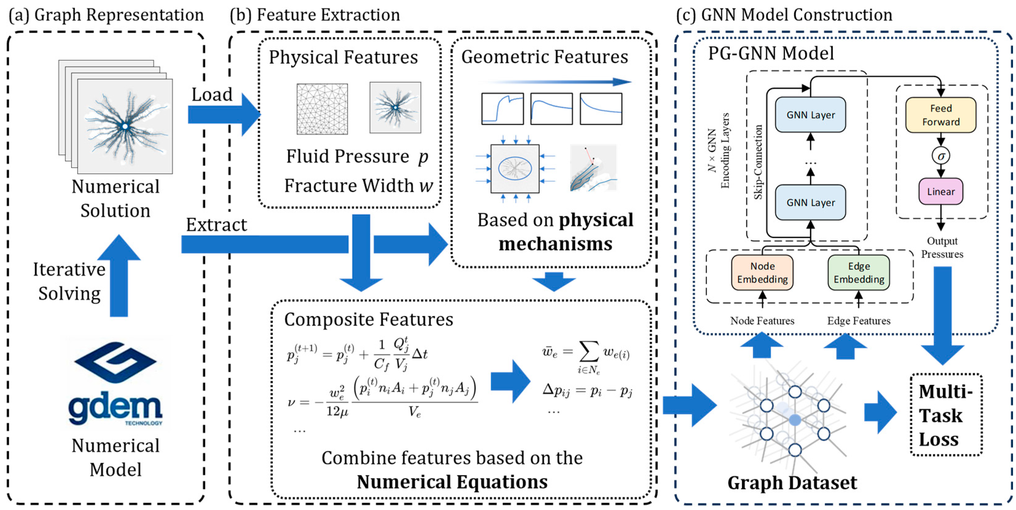
To provide a coherent formulation, the proposed PG-GNN-based framework follows a unified workflow consisting of three components. First, numerical simulation outputs from the CDEM based solver are converted into a graph representation that preserves the spatial topology of the reservoir and the connectivity of fracture elements. Second, physics-guided features derived from governing fracture-flow equations (see Equation (4)), geometric relationships, and fracture-flow characteristics are constructed on nodes and edges. Finally, these features are processed by a multi-layer GNN architecture designed to emulate the iterative nature of pressure transmission, with a prediction head that outputs the pressure at the next time step. In addition, the graph formulation is independent of mesh regularity, allowing the method to operate on both structured and unstructured reservoir discretization. The overall architecture is illustrated in Figure 2, and the detailed formulation of each component is presented in Section 3.1, Section 3.2, Section 3.3 and Section 3.4.

3.1. Graph-Based Representation

Following the reservoir partitioning strategy used in the CDEM-based numerical model, the reservoir in this study is represented as a graph structure $\mathcal{G}=⟨\mathcal{V},\mathcal{E}⟩$ constructed directly from the simulation mesh. As described in Section 2, the CDEM based numerical solver provides high-resolution fields of fluid pressure, displacement, and fracture width on an irregular triangular mesh, with locally refined elements near the wellbore to better capture the rapid dynamics of deflagration fracturing. This subsection focuses on how the numerical data are mapped to a graph representation suitable for GNN-based learning.

Nodes $\mathcal{V}$ correspond to vertices of the simulation mesh and represents spatial locations where pressure and other state variables are evaluated. Edges $\mathcal{E}$ represents the interfaces between adjacent node, corresponding to fracture segments or potential propagation paths within the reservoir. Each edge carries geometric and physical attributes including element length, orientation, and equivalent fracture width. By inheriting the connectivity and spatial layout of the original mesh, the constructed graph faithfully preserves the irregular topology of the CDEM discretization.

This graph-centered formulation does not rely on any assumption of grid regularity. Because the PG-GNN operates solely through node-edge connectivity by message passing mechanism [30] rather than fixed convolutional stencils, the method is naturally accommodates both structured (regular) and unstructured (irregular) mesh. As a result, the framework accommodates the irregular triangular grid produced by CDEM and can be applied without modification to other numerical discretization commonly used in reservoir simulation.

3.2. Physics-Guided Feature Construction

To enhance the ability of graph neural networks to model fracture seepage processes, this study incorporates both the underlying physical mechanisms of deflagration fracturing and key variables from numerical simulations during the feature engineering stage. The overall feature design includes geometric features, physical features, and composite features derived from the governing equations of fracture flow (Equation (4)), enabling the model to learn the evolution of fluid pressure under physical guidance within a data-driven framework.

3.2.1. Physical Features

In deflagration fracturing, except for the early stage (approximately 1 to 2 milliseconds) dominated by the explosive impact, the subsequent evolution is primarily governed by the fracture seepage equations, exhibiting transient pressure transmission and fracture propagation behavior.

Therefore, this study selects the following two key physical quantities from the fracture flow mechanism to construct physical features.

(1)

Fluid pressure at the previous time step, $p_{t-1}$

Fluid pressure is the core variable driving fracture propagation and seepage, which directly reflects the pressure at a given location in the reservoir at the previous time step, serving as the fundamental input for predicting subsequent pressure evolution. In this work, it is defined as a node-level feature.

(2)

Equivalent fracture width, $w_e$

This geometric property appears in the governing equation of seepage as a key variable influencing flow velocity. Physically, a larger $w_e$ indicates stronger permeability and faster fluid transmission under a given pressure gradient. This feature is assigned to edges in the graph.

3.2.2. Geometric Features

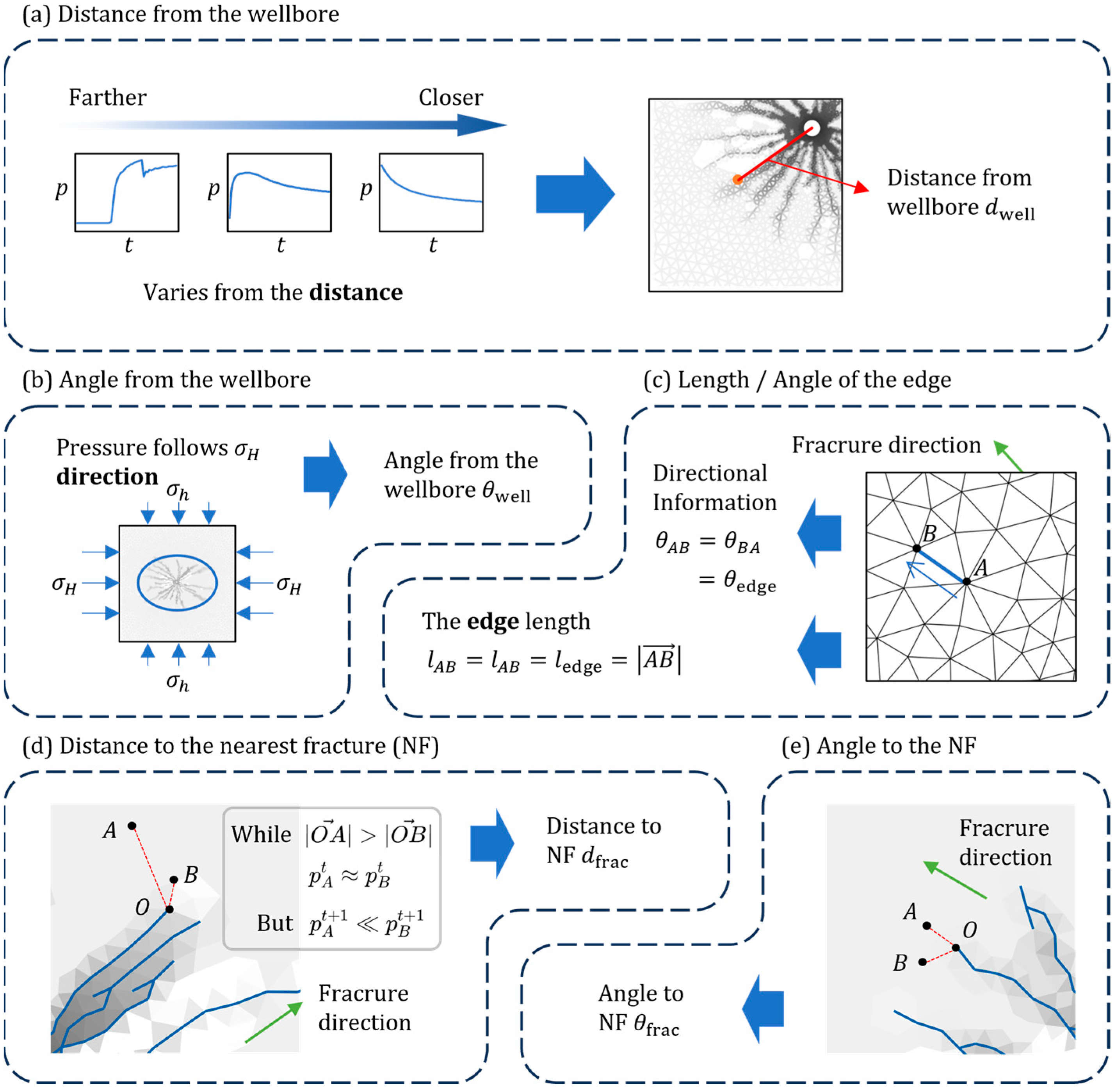
During deflagration fracturing, the seepage behavior is closely related to the distribution characteristics of the fluid pressure field. To capture information such as fracture propagation direction, fluid flow paths, and the influence of in situ stress, we design the following geometric features based on the spatial configuration of fractures, as illustrated in Figure 3.

(1)

Distance from the Wellbore, $d_{\mathrm{well}}$

The deflagration source is located within the wellbore, and the pressure distribution in the reservoir typically exhibits a radial pattern centered around this point. As shown in Figure 3a, nodes closer to the wellbore experience higher initial pressures that decrease over time, while nodes farther away exhibit a rise-then-fall pressure trend due to delayed fluid seepage, reflecting the spatial relationship between each node and the blast center. This feature helps the model learn pressure evolution patterns based on spatial positioning.

(2)

Angle between the line connecting the node and the wellbore center and the direction of maximum horizontal stress ${\sigma }_H$, denoted ${\theta }_{\mathrm{well}}$

This angular feature captures the influence of in situ stress orientation on fluid flow paths. Due to the non-uniform initial stress field in the formation, fluid tends to flow along the direction of maximum principal stress during seepage, resulting in anisotropic fracture propagation ranges in different directions, as shown in Figure 3b. This feature enables the model to learn the impact of in situ stress orientation on flow evolution paths.

(3)

Edge length $l_{\mathrm{edge}}$ and orientation ${\theta }_{\mathrm{edge}}$

The edge length directly reflects the geometric scale of a fracture unit and is closely related to flow imbalance during seepage. This feature improves the model sensitivity to local variations in spatial permeability. Meanwhile, edge orientation characterizes the directional nature of the fracture unit, facilitating learning of directional fracture propagation, as illustrated in Figure 3c.

(4)

Minimum distance between a node and the nearest fracture path, $d_{\mathrm{frac}}$

This feature captures the proximity of a node to the nearest fracture tip, which is crucial for understanding local pressure gradients. As shown in Figure 3d, nodes closer to fracture tips typically experience higher pressure gradients due to fluid accumulation and flow dynamics near the propagation front. This feature helps the model learn local pressure variations influenced by fracture geometry.

(5)

Relative angle between a node and the adjacent fracture path, ${\theta }_{\mathrm{frac}}$

This feature reflects the spatial orientation between a node and the nearest fracture path. As illustrated in Figure 3e, even with similar pressure values, fractures tend to propagate along the current extension direction rather than perpendicularly. This feature enhances the model’s directional awareness of fluid propagation.

3.2.3. Physics-Guided Composite Features

To further enhance the model capability in capturing the nonlinear evolution of fracture seepage, this study constructs a set of physics-guided composite features based on the iterative form of the governing equations in deflagration fracture flow (Equation (4)). The iterative solution using the explicit Euler forward scheme is formulated as follows:

$$p_j^{\left(t+1\right)}=p_j^{\left(t\right)}+{\displaystyle \frac{1}{C_f}}{\displaystyle \frac{Q_j^t}{V_j}}\Delta t$$

(5)

where $Q_j^{\left(t\right)}$ denotes the total inflow at node $j$, computed by summing the flow rates from adjacent fracture elements:

$$Q_j^{\left(t\right)}=\sum _{i\in N_e}{q}_i^{\left(t\right)}$$

(6)

The instantaneous flow rate through fracture element $i$, denoted $q_i^{\left(t\right)}$, is given by:

$$q_i^{\left(t\right)}=\left(\nu \cdot {\overrightarrow{n}}_i\right)A_i$$

(7)

where $\nu$ is the seepage velocity along the fracture edge, calculated as:

$$\nu =-{\displaystyle \frac{w_e^2}{12\mu }}{\displaystyle \frac{\left(p_i^{\left(t\right)}{n}_i{A}_i+p_j^{\left(t\right)}{n}_j{A}_j\right)}{V_e}}$$

(8)

where $V_e$ is the volume of the fracture element, $p_j^{\left(t\right)}$ and $p_i^{\left(t\right)}$ are pressures at the two ends, $A_i$ and $A_j$ are the corresponding cross-sectional areas, and $n_i$, $n_j$ are the respective normal vectors.

Based on the above formulation, we construct the following physically meaningful composite features:

(1)

Fluid pressure difference on edge, $\Delta p_{ij}$

This variable is the primary driving force for fracture flow, corresponding to the pressure gradient term $\nabla p$ in the governing equation, and represents the instantaneous pressure drop between nodes $i$ and $j$. It is calculated as $\Delta p_{ij}=p_i-p_j$ and assigned to edges.

(2)

Coupled pressure-width term, $p\cdot w_e^2$

According to the seepage velocity formula (Equation (8)), the square of the fracture width is proportional to flow velocity. This term reflects the fluid conductance under unit pressure, enhancing nonlinear expressiveness.

(3)

Projected pressure difference along fracture direction, $\Delta {\overrightarrow{p}}_{\parallel ij}$

This component quantifies the effective pressure difference in the actual flow direction and serves as a critical directional cue in the message-passing process along graph edges. It is computed as:

$$\Delta {\overrightarrow{p}}_{\parallel ij}=\Delta p_{ij}\cdot {\overrightarrow{n}}_{\mathrm{edge}}$$

(9)

(4)

Average fracture width in node neighborhood, ${\bar{w}}_e$

This feature captures the average fracture width in the local neighborhood of a node, reflecting the local permeability characteristics. It is computed as:

$${\bar{w}}_e={\displaystyle \frac{1}{\left|N_e\right|}}\sum _{i\in N_e}{w}_{e,i}$$

(10)

where $N_e$ denotes the set of edges connected to the node.

These composite features ensure consistency between the model inputs and the physical process of fracture seepage, making them highly compatible with the message-passing framework of GNNs, and thereby improving the model ability to capture complex fluid–structure interactions.

For completeness,

Table 1. Summary of node-level and edge-level features used in the PG-GNN.

Feature Type	Description	Symbol
Node-Level	Fluid pressure at the previous time step	$p_{t-1}$
	Distance from the wellbore	$d_{\mathrm{well}}$
	Angle between the line connecting the node and the wellbore center and the direction of maximum horizontal stress ${\sigma }_H$	${\theta }_{\mathrm{well}}$
	Minimum distance between a node and the nearest fracture path	$d_{\mathrm{frac}}$
	Relative angle between a node and the adjacent fracture path	${\theta }_{\mathrm{frac}}$
	Average fracture width in node neighborhood,	${\bar{w}}_e$
Edge-Level	Equivalent fracture width	$w_e$
	Edge length	$l_{\mathrm{edge}}$
	Edge orientation	${\theta }_{\mathrm{edge}}$
	Fluid pressure difference on edge	$\mathit{\Delta }{p}_{ij}$
	Coupled pressure-width term	$p\cdot w_e^2$
	Projected pressure difference along fracture direction	$\mathit{\Delta }{\overrightarrow{p}}_{\parallel ij}$

provides a consolidated summary of all node-level and edge-level features employed in the PG-GNN framework.

3.3. PG-GNN Architecture

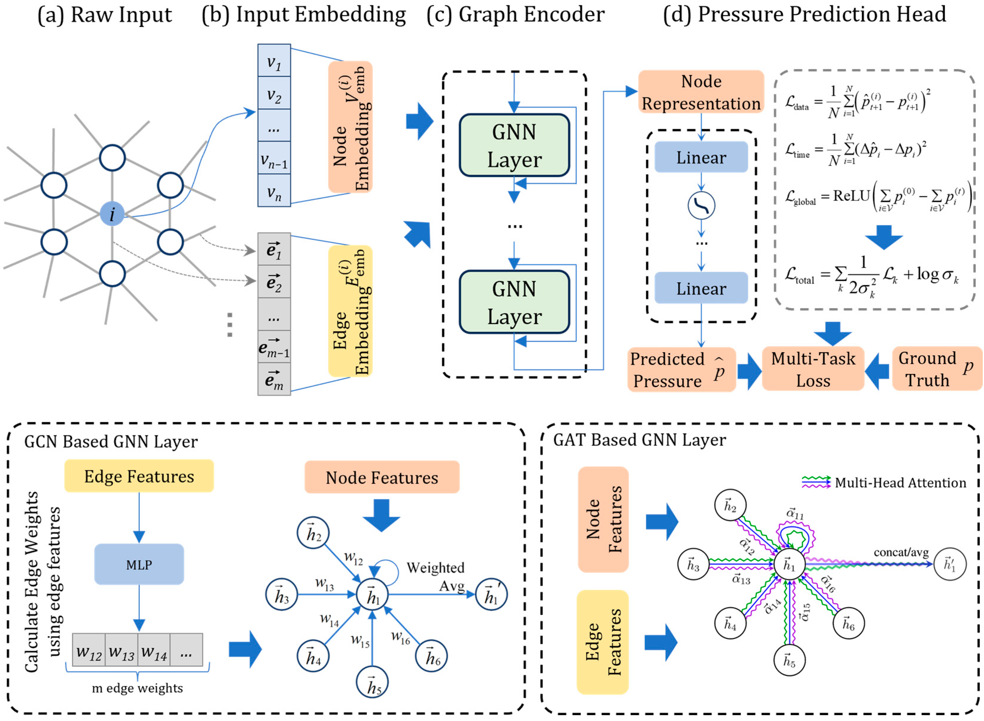
The PG-GNN adopts a multi-layer message passing architecture designed to capture the local propagation of fluid pressure across the fracture network. The architecture consists of these components: (1) an input embedding layer that transforms node and edge features into latent representations, (2) a graph encoder that performs iterative message passing, and (3) a fluid pressure prediction head that outputs the fluid pressure at the next time step. This structure mirrors the physical process in which pressure redistribution propagates along fracture connections. The PG-GNN model architecture is illustrated in Figure 4.

The following sections describe the structure and functionality of each module in detail.

3.3.1. Input Embedding

Let $X_v\mathsf{ϵ}{\mathbb{R}}^{d_v}$ and $X_e\mathsf{ϵ}{\mathbb{R}}^{d_e}$ denotes the raw node and edge feature vector described in Section 3.2. The input embedding layer includes separate embedding modules for node features and edge features. It projects the raw node and edge features into a unified high-dimensional space via linear transformation layers:

$$H_v^{\left(0\right)}=W_v{X}_v+{\theta }_v,H_e^{\left(0\right)}=W_e{X}_e+{\theta }_e$$

(11)

where $W_v$, $W_e$, ${\theta }_v$, and ${\theta }_e$ are learnable matrices. This embedding step aligns the heterogeneous physical descriptors into a common latent space suitable for message passing, which serve as the initial representations for subsequent graph neural network propagation.

3.3.2. Graph Encoder

(1)

Overall Structure

The graph encoder serves as the core of the model and comprises $L$ stackedGNN layers with skip connections, where each GNN layer facilitates message passing and feature aggregation across the graph, and skip connections are introduced to mitigate the over-smoothing effect caused by deep stacking of GNN layers [31].

(2)

Multi-Layer GNN

The graph encoder consists of multiple stacked GNN layers that perform node-wise information exchange and representation updating over the graph. In this work, we consider two alternative architectures for the GNN layer: a modified Graph Convolutional Network (GCN) and the Graph Attention Network (GAT).

The original GCN model is structurally simple and computationally efficient, making it well-suited for large-scale graphs [32,33]. However, its mean-based neighbor aggregation mechanism limits its capacity in modeling graphs with heterogeneous information distributions. To address this, we incorporate edge-weighted mechanisms into the GCN to better capture structural heterogeneity. Nonetheless, the current scheme allows only scalar edge weights, which still constrains its expressiveness.

In contrast, the GAT model leverages attention mechanisms to assign learnable, non-uniform weights to neighboring nodes, offering higher adaptability, especially for graphs with complex and heterogeneous topologies. However, the increased computational cost and memory usage may pose practical challenges during training.

Therefore, both architectures are implemented and evaluated as candidates for the graph encoder. Given their respective strengths and weaknesses, it is difficult to determine their relative performance a priori for this specific task, and comparative analysis will be performed in the experimental section.

(3)

GNN Layer Based on Modified GCN

The message-passing mechanism of the original GCN is based on a normalized Laplacian matrix that transforms node features through linear propagation [30]. The process can be expressed as follows.

$${\mathbf{H}}^{\left(l+1\right)}=\sigma \left({\tilde{\mathbf{D}}}^{-{\displaystyle \frac{1}{2}}}\tilde{\mathbf{A}}{\tilde{\mathbf{D}}}^{-{\displaystyle \frac{1}{2}}}{\mathbf{H}}^{\left(l\right)}{\mathbf{W}}^{\left(l\right)}\right)$$

(12)

where $\tilde{A}=A+I_N$ is the adjacency matrix with self-loops, $\tilde{D}$ is the corresponding degree matrix, and $W^{\left(l\right)}$ is the trainable weight matrix at layer $l$.

Edge features are incorporated into the original GCN by adopting ideas from the attention mechanisms [34,35], where fixed adjacency weights are replaced with learnable weights derived from the edge features. Specifically, for a node $i$ and its neighbor $j$, the edge weight is defined as:

$${\alpha }_{ij}={\displaystyle \frac{\mathrm{e}\mathrm{x}\mathrm{p}\left(\sigma \left({\mathbf{a}}^{\mathrm{T}}\mathrm{L}\mathrm{i}\mathrm{n}\mathrm{e}\mathrm{a}\mathrm{r}\left(e_{ij}\right)\right)\right)}{\sum _{k\in \mathcal{N}\left(i\right)}\mathrm{e}\mathrm{x}\mathrm{p}\left(\sigma \left({\mathbf{a}}^T\mathrm{L}\mathrm{i}\mathrm{n}\mathrm{e}\mathrm{a}\mathrm{r}\left(e_{ik}\right)\right)\right)}}$$

(13)

The resulting edge weights are used to construct a weighted adjacency matrix $A_{\mathrm{weighted}}$, which replaces the standard adjacency matrix in the GCN propagation process. The modified GCN layer can then be expressed as follows:

$${\mathbf{H}}^{\left(l+1\right)}=\sigma \left({\mathbf{D}}^{-{\displaystyle \frac{1}{2}}}{A}_{\mathrm{weighted}}{\mathbf{D}}^{-{\displaystyle \frac{1}{2}}}{\mathbf{H}}^{\left(l\right)}{\mathbf{W}}^{\left(l\right)}\right)$$

(14)

This allows the model to effectively fuse both structural and physical attributes of edges, enhancing its capacity to model fluid transport and pressure dynamics.

(4)

GNN Layer Based on GAT

Graph Attention Networks (GATs) [34] are spatial-based GNN architectures that utilize attention mechanisms to assign different importance to neighboring nodes. The core idea is to compute attention coefficients for each edge in the graph, allowing the model to focus on the most relevant neighbors during message passing.

For any node $i\in \mathcal{V}$, the GAT layer computes the attention coefficients ${\alpha }_{ij}$ with respect to each neighbor $j$ is computed as follows.

$${\alpha }_{ij}={\displaystyle \frac{\mathrm{e}\mathrm{x}\mathrm{p}\left(\mathrm{LeakyReLU}\left({\mathbf{a}}^T\left[W_1{h}_i\parallel W_2{h}_j\parallel W_3{e}_{ij}\right]\right)\right)}{\sum _{k\in \mathcal{N}\left(i\right)}\mathrm{e}\mathrm{x}\mathrm{p}\left(\mathrm{LeakyReLU}\left({\mathbf{a}}^T\left[W_1{h}_i\parallel W_2{h}_k\parallel W_3{e}_{ik}\right]\right)\right)}}$$

(15)

where ${\mathbf{h}}_i$, ${\mathbf{h}}_j$ are the node features, and ${\mathbf{e}}_{ij}$ denotes the edge feature. $W_1,W_2,W_3$ are learnable transformation matrices, and $\mathbf{a}$ is the attention vector, and $\parallel$ debnotes concatenation, which can be replaced with element-wise multiplication if desired.

Then, node features are updated by aggregating the features of neighboring nodes weighted by the attention coefficients, which can be expressed as follows.

$${\mathbf{H}}_i^{\left(l+1\right)}=\sigma \left(\sum _{j\in \mathcal{N}\left(i\right)}{\alpha }_{ij}{\mathbf{W}}^{\left(l\right)}{\mathbf{h}}_j^{\left(l\right)}\right)$$

(16)

By explicitly incorporating node and edge features, GAT enables more accurate modeling of physics-guided fracture flow behaviors.

(5)

Skip Connections

To alleviate the over-smoothing effect caused by deep message passing in GNNs, and to enhance the expressiveness of each layer, the skip connection mechanism is incorporated at each GNN layer. Specifically, the output of each GNN layer is fused with its corresponding input feature via residual connection, which can be expressed as follows.

$${\mathbf{H}}^{\left(l+1\right)}={\mathbf{H}}^{\left(l\right)}+{\mathrm{GNN}}^{\left(l\right)}\left({\mathbf{H}}^{\left(l\right)},{\mathbf{E}}^{\left(l\right)}\right)$$

(17)

Here, ${\mathbf{h}}^{\left(l\right)}$ denotes the input to the $l$-th GNN layer, and ${\mathrm{G}\mathrm{N}\mathrm{N}}^{\left(l\right)}$ represents the GNN operation at layer $l$.

This design enables joint modeling of both shallow and deep-level representations. This mechanism not only helps to mitigate the vanishing gradient issue, but also preserves essential geometric and physical information captured at lower layers during training.

By integrating skip connections at each layer, the model effectively mitigates feature degradation, preserves essential geometric and physical information, and enhances the overall expressiveness of the GNN architecture, leading to improved training stability and generalization in deep GNN architectures.

3.3.3. Pressure Prediction Head

This module is responsible for mapping the encoded node representations to the predicted fluid pressure at the next time step, thereby enabling dynamic modeling of the evolving pressure field during deflagration fracturing. In addition, given that the initial features contain rich physical information and geometric priors, a skip connection is introduced between the initial node embeddings and the prediction head, which fuses the initial embeddings with the final outputs of the graph encoder, allowing the model to leverage both learned representations and original features for improved prediction accuracy. This skip connection can be mathematically formulated as follows.

$${\mathbf{H}}^{\left(\mathrm{fused}\right)}={\mathbf{H}}^{\left(\mathrm{embed}\right)}+{\mathbf{H}}^{\left(\mathrm{final}\right)}$$

(18)

Here, ${\mathbf{h}}^{\left(\mathrm{embed}\right)}\in {\mathbb{R}}^{N\times d}$ denotes the initial node embeddings, and ${\mathbf{h}}^{\left(\mathrm{final}\right)}$ represents the output of the graph encoder.

The fused representation is then fed into a multi-layer perceptron (MLP) for decoding, which outputs the fluid pressure prediction for each node at the next time step. The prediction head consists of three linear transformations interleaved with activation functions, which balances representation capacity with reduced risk of overfitting. The final output serves as the target in the loss function computation, enabling joint optimization of the model’s predictive performance and physical consistency via a multi-task loss formulation.

3.4. Optimization Objectives

The PG-GNN is trained to predict the fluid pressure at the next time step, to improve the prediction accuracy, physical consistency, and temporal stability of the model, a multi-task loss function that integrates multiple error components is designed, each addressing a different aspect of fluid pressure evolution during deflagration fracturing. The components are as follows:

(1)

Data Loss

The basic data loss term is the Mean Squared Error (MSE), which is designed to minimize the discrepancy between the predicted and true fluid pressures at each node in the fracture network. This loss function helps the model improve prediction accuracy by penalizing large deviations from the observed pressure values. Specifically, the data loss term is formulated as:

$${\mathcal{L}}_{\mathrm{data}}={\displaystyle \frac{1}{N}}\sum _{i=1}^N{\left({\widehat{p}}_{t+1}^{\left(i\right)}-p_{t+1}^{\left(i\right)}\right)}^2$$

(19)

where ${\widehat{p}}_{t+1}^{\left(i\right)}$ is the predicted pressure and $p_{t+1}^{\left(i\right)}$ is the true pressure at node $i$ at time $t+1$.

(2)

Temporal Difference Constraint

In deflagration fracturing, fluid pressure exhibits both gradual changes and abrupt variations, particularly during fracture propagation. The Temporal Difference Constraint is introduced not only to enforce temporal consistency but also to allow the model to learn and capture the changing trends of fluid pressure, especially the sudden pressure spikes or discontinuities caused by fracture propagation.

Rather than solely penalizing smooth pressure evolution between time steps, this constraint helps the model identify and replicate abrupt pressure variations that occur as fractures expand within the reservoir. These pressure changes are inherently linked to fracture propagation, where the pressure in the network can undergo sudden jumps due to the creation of new fracture paths or the reconfiguration of existing fractures.

$${\mathcal{L}}_{\mathrm{time}}={\displaystyle \frac{1}{N}}\sum _{i=1}^N{\left(\Delta {\widehat{p}}_i-\Delta p_i\right)}^2$$

(20)

where $\Delta p_i=p_i^{\left(t\right)}-p_i^{(t-1)}$ denotes the pressure difference at node $i$ between consecutive time steps, and $\Delta {\widehat{p}}_i$ is the predicted pressure difference.

This constraint enforces the model to not only learn smooth temporal transitions but also to capture the discontinuities and abrupt shifts in pressure as a result of fracture initiation and propagation.

(3)

Global Pressure Constraint

According to physical principles, the total fluid pressure in a reservoir undergoing deflagration fracturing is expected to decrease gradually due to energy dissipation and fluid flow. The global pressure constraint ensures that the total pressure over the entire graph does not exceed the initial value at any time step. This is in accordance with the energy dissipation inherent in fracturing processes, where the energy contained in the system is progressively released, leading to a reduction in pressure over time.

The global pressure loss is defined as:

$${\mathcal{L}}_{\mathrm{global}}=\mathrm{ReLU}\left(\sum _{i\in \mathcal{V}}{p}_i^{\left(t\right)}-\sum _{i\in \mathcal{V}}{p}_i^{\left(t+1\right)}\right)$$

(21)

where $p_i^{\left(t\right)}$ is the fluid pressure at node i at time step t. The ReLU function ensures that the loss is only activated when the total pressure exceeds the initial value.

$$\mathrm{ReLU}\left(x\right)=\mathrm{m}\mathrm{a}\mathrm{x}\left(0,x\right)$$

(22)

(4)

Uncertainty-Weighted Loss Integration

To balance the importance of different tasks and improve convergence stability, we adopt an uncertainty-based loss weighting scheme [36], where each task loss is weighted by a learned uncertainty parameter ${\sigma }_k$, which allows the model to adjust the emphasis on each objective according to the uncertainty of the model’s predictions.

The total loss function is therefore formulated as:

$${\mathcal{L}}_{\mathrm{total}}=\sum _k{\displaystyle \frac{1}{2{\sigma }_k^2}}{\mathcal{L}}_k+\mathrm{l}\mathrm{o}\mathrm{g}{\sigma }_k$$

(23)

where ${\mathcal{L}}_k$ denotes the $k$-th task loss (e.g., data, temporal or global), and ${\sigma }_k$ is the learned uncertainty parameter for task $k$.

The overall loss function combines the data loss, temporal difference loss, and global pressure loss, each weighted by the uncertainty parameter. This formulation allows the model to effectively learn the spatiotemporal dynamics of fluid pressure evolution while maintaining consistency with physical laws governing deflagration fracturing. The multi-task loss function, coupled with uncertainty weighting, ensures that the model balances prediction accuracy with physical realism, promoting both model robustness and realistic predictions.

4. Experiments and Results

4.1. Dataset and Data Preparation

The dataset used in this study is derived from a two-dimensional deflagration fracturing numerical model based on the CDEM [10]. This model simulates the propagation of rock fractures driven by deflagration on a 2D mesh using an explicit dynamic iterative solver, while simultaneously coupling the transient flow of high-pressure gas within the fracture network.

In our experiments, a 2D reservoir domain of size $10\mathrm{m}\times 10\mathrm{m}$ is constructed, with a circular region of radius $0.08\mathrm{m}$ at the center of the domain representing the wellbore location for deflagration fracturing. Then, the reservoir is discretized into a triangular mesh, where smaller elements ($0.015\mathrm{m}$) are used near the wellbore to enhance resolution, while larger elements ($0.25\mathrm{m}$) are applied near the model boundary to accelerate computation. To ensure physical relevance, the $10\mathrm{m}\times 10\mathrm{m}$ simulation domain was chosen to exceed the typical 2–5 m effective stimulation radius observed in single-event deflagration fracturing, allowing the full near-wellbore fracture process to be captured. The key physical and material parameters used in the simulation are listed in

Table 2. Model Parameters Used in CDEM Simulation.

Parameter	Value
Model Length	10 m
Model Width	10 m
Wellbore Radius	0.08 m
Rock Density	2600 kg⋅m−3
Elastic Modulus	40 GPa
Poisson’s Ratio	0.2
Cohesive Strength	30 MPa
Tensile Strength	10 MPa
Internal Friction Angle	45°
Charge Density	50 kg⋅m−3
Detonation Velocity	400 m⋅s−1
Detonation Heat	3 × 107 J⋅kg−1
$\mathrm{Horizontal}\mathrm{Stress}{\mathsf{\sigma }}_{\mathrm{H}}$	50 MPa
$\mathrm{Horizontal}\mathrm{Stress}{\mathsf{\sigma }}_{\mathrm{h}}$	40 MPa

.

The simulation spans a physical time period of 135 milliseconds, recorded with each time step of 0.225 milliseconds, resulting in a total of 600 sequential time steps. At each time step, the fluid pressure field, displacement field, and fracture width data are exported, capturing the complex interactions between the solid matrix and the fluid phase, ensuring the dataset forms a continuous, uniformly sampled time series. All snapshots are used consecutively without skipping, subsampling or interpolation.

To convert the numerical simulation outputs into structured data suitable for processing by a graph neural network, we map the physical field data obtained from the numerical model, namely fluid pressure in the fracture seepage field, displacement field, and fracture aperture, into a graph representation at each sampled time step.

For each sampled timestep $t$, the graph structure ${\mathcal{G}}_t=⟨{\mathcal{V}}_t,{\mathcal{E}}_t⟩$ is constructed as follows:

(1)

The node set ${\mathcal{V}}_t$ consists of all nodes in the triangular mesh, where each node represents a spatial location in the reservoir domain.

(2)

The edge set ${\mathcal{E}}_t$ is constructed based on the connectivity of the triangular mesh, where each edge connects two adjacent nodes in the mesh.

(3)

Both nodes and edges carry the physical field information specifies to the timestep $t$, including the features described in Section 3.2, such as fluid pressure, equivalent fracture width, and geometric features.

The adjacency structure of the graph remains fixed across time steps, reflecting the topological structure of the triangular mesh in the numerical model and ensuring spatial consistency. In the temporal dimension, the Markov-like structure arises directly from the explicit time-integration scheme used in the CDEM solver, where the state at time $t+\mathit{\Delta }t$ is computed solely from the state at time $t$. History-dependent effects such as stress redistribution and stress shadowing are already encoded in the updated displacement, aperture, and pressure fields at each step. Therefore, the Markov assumption used here follows standard practice in explicit fracture dynamics simulations and represents a first-order temporal approximation rather than the claim that the physical system has no memory. A supervised learning framework is adopted to predict the fluid pressure at the next time step based on the current graph features, thereby enabling end-to-end learning.

4.2. Experiment Settings

4.2.1. Evaluation Metrics

In this study, we evaluate the model performance using Mean Absolute Percentage Error (MAPE) and Mean Squared Error (MSE) as the primary metrics to evaluate the regression performance of our models in predicting node-wise fluid pressure in deflagration fracturing.

MAPE measures the relative error between predicted and true values and is unit-free, making it suitable for performance comparison across different data scales, which is defined as:

$$\mathrm{M}\mathrm{A}\mathrm{P}\mathrm{E}={\displaystyle \frac{1}{N}}\sum _{i=1}^N\left|{\displaystyle \frac{y_i-{\widehat{y}}_i}{y_i}}\right|$$

(24)

where $y_i$ is the ground truth fluid pressure at node $i$, ${\widehat{y}}_i$ is the predicted value, and $N$ is the total number of nodes.

Additionally, the MSE loss is employed to capture the average of squared errors, which is more sensitive to large deviations and better reflects the influence of outliers on model performance. Its definition is as follows.

$$\mathrm{M}\mathrm{S}\mathrm{E}={\displaystyle \frac{1}{N}}\sum _{i=1}^N{\left(y_i-{\widehat{y}}_i\right)}^2$$

(25)

By combining MAPE and MSE, a robust evaluation framework that captures both average deviations and abnormal fluctuations in prediction performance has been established, providing a comprehensive assessment of the model’s predictive capabilities. While MAPE offers a normalized assessment of prediction accuracy, MSE emphasizes the impact of large errors, making them complementary metrics for evaluating fluid pressure evolution in deflagration fracturing.

4.2.2. Baselines

To validate the effectiveness of the proposed method, following baseline models are selected for comparison:

(1)

MLP: A fully connected multilayer perceptron model that only takes node features as input. Due to its lack of graph structure modeling and physical constraints, the MLP is trained solely using the data loss term.

(2)

Pure GCN: A Graph Convolutional Network model consisting only of graph encoding layers, which uses both node and edge features as input. The GCN is trained with the full loss function, including the data loss, temporal difference constraint, and global pressure constraint. This model serves as a baseline to assess the effectiveness of the physics-guided components.

4.3. Results

4.3.1. Overall Performance

Figure 5, Figure 6 and Figure 7 illustrate the predicted fluid pressure distributions at time steps t = 200, t = 400, and t = 500, respectively. These results provide a visual comparison of the model’s performance on the training, validation, and test datasets.

Figure 5a,b present the ground truth and prediction results on the training set, respectively. The predicted pressure distribution closely matches the actual values, capturing both the overall trend and fine-scale variations across the domain. As shown in Figure 5c, which illustrates the residuals between predicted and ground-truth pressures, the overall prediction error on the training set is minimal. The majority of the residuals are concentrated within $\pm 0.5\mathrm{MPa}$, indicating high prediction accuracy. The maximum residual is approximately $3.218\mathrm{MPa}$, which occurs in localized regions with sharp pressure gradients. Similar agreement between predictions and ground truth is observed on the validation and test sets, as shown in Figure 6 and Figure 7, respectively, indicating consistent performance across all data splits.

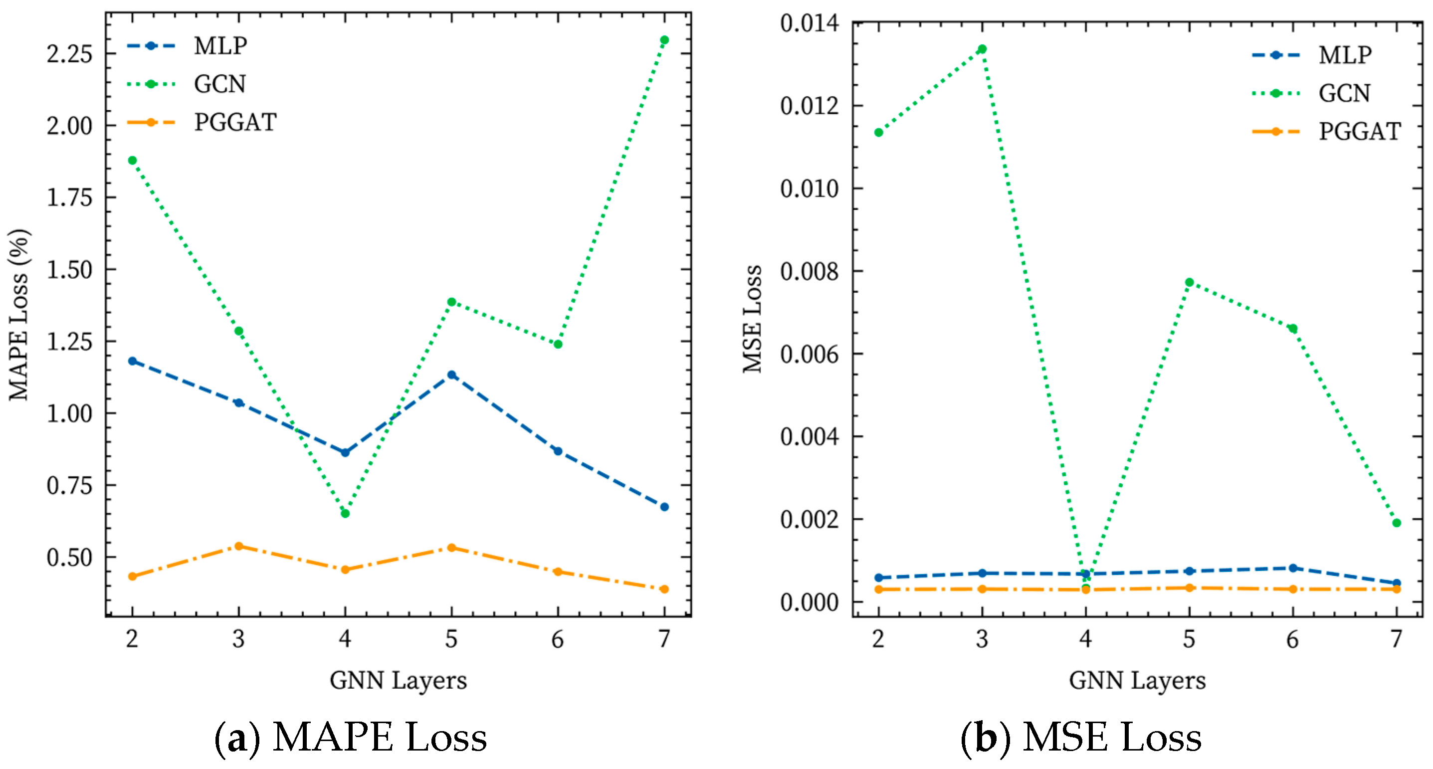
Figure 8 presents a performance comparison between the proposed method and baseline models, along with the impact of varying the number of neural network layers on model performance.

In this experiment, all models are configured with 64 neurons per hidden layer. The Adam optimizer is used with an initial learning rate of 0.001. A learning rate scheduler is employed to reduce the learning rate by half if the validation loss does not improve for 5 consecutive epochs. The maximum number of training epochs is set to 200. As shown in the figure, across all settings of neural network depth, the proposed method consistently achieves higher prediction accuracy, with lower values in both MSE and MAPE. As the number of neural network layers increases, the performance of the proposed method initially improves and then stabilizes. The best performance is observed when using 5 GNN layers. Under this setting, the proposed method outperforms the MLP and pure GCN models by 1.047% and 1.074%, respectively. In addition, the proposed model exhibits significantly better robustness compared to the baselines. For instance, when the number of GNN layers is fixed at 5, the standard deviation of the proposed model is only 0.043, whereas that of the MLP and GCN models are 0.210 and 0.519, respectively. Detailed performance metrics are provided in

Table 3. Comparison of MSE and MAPE (%) on the Validation Set under Different GNN Layers.

Layers	MSE			MAPE
	MLP	GCN	Proposed	MLP	GCN	Proposed
2	$5.838\times {10}^{-4}$	$1.135\times {10}^{-2}$	$\mathbf{3.020}\times {\mathbf{10}}^{-\mathbf{4}}$	1.181%	1.879%	0.433%
3	$6.938\times {10}^{-4}$	$1.337\times {10}^{-2}$	$\mathbf{3.090}\times {\mathbf{10}}^{-\mathbf{4}}$	1.036%	1.286%	0.538%
4	$6.750\times {10}^{-4}$	$3.340\times {10}^{-4}$	$\mathbf{2.930}\times {\mathbf{10}}^{-\mathbf{4}}$	0.863%	0.651%	0.456%
5	$7.425\times {10}^{-4}$	$7.728\times {10}^{-3}$	$\mathbf{3.400}\times {\mathbf{10}}^{-\mathbf{4}}$	1.134%	1.387%	0.533%
6	$8.175\times {10}^{-4}$	$6.614\times {10}^{-3}$	$\mathbf{3.070}\times {\mathbf{10}}^{-\mathbf{4}}$	0.868%	1.239%	0.449%
7	$4.513\times {10}^{-4}$	$1.909\times {10}^{-3}$	$\mathbf{3.060}\times {\mathbf{10}}^{-\mathbf{4}}$	0.674%	2.297%	0.388%

.

4.3.2. Hyperparameter Analysis

In this study, we investigate three categories of hyperparameters based on the PG-GAT model, a variant of the proposed method that utilizes GAT layers for graph encoding, including the number of hidden neurons per layer, the number of attention heads in GAT, and the number of GNN layers. Specifically, the number of hidden neurons is chosen from the set 32, 64, 96, 128, the number of GAT attention heads is varied within 2, 4, 6, 8, 12, 16, and the number of GNN layers is tested from 2 to 7.

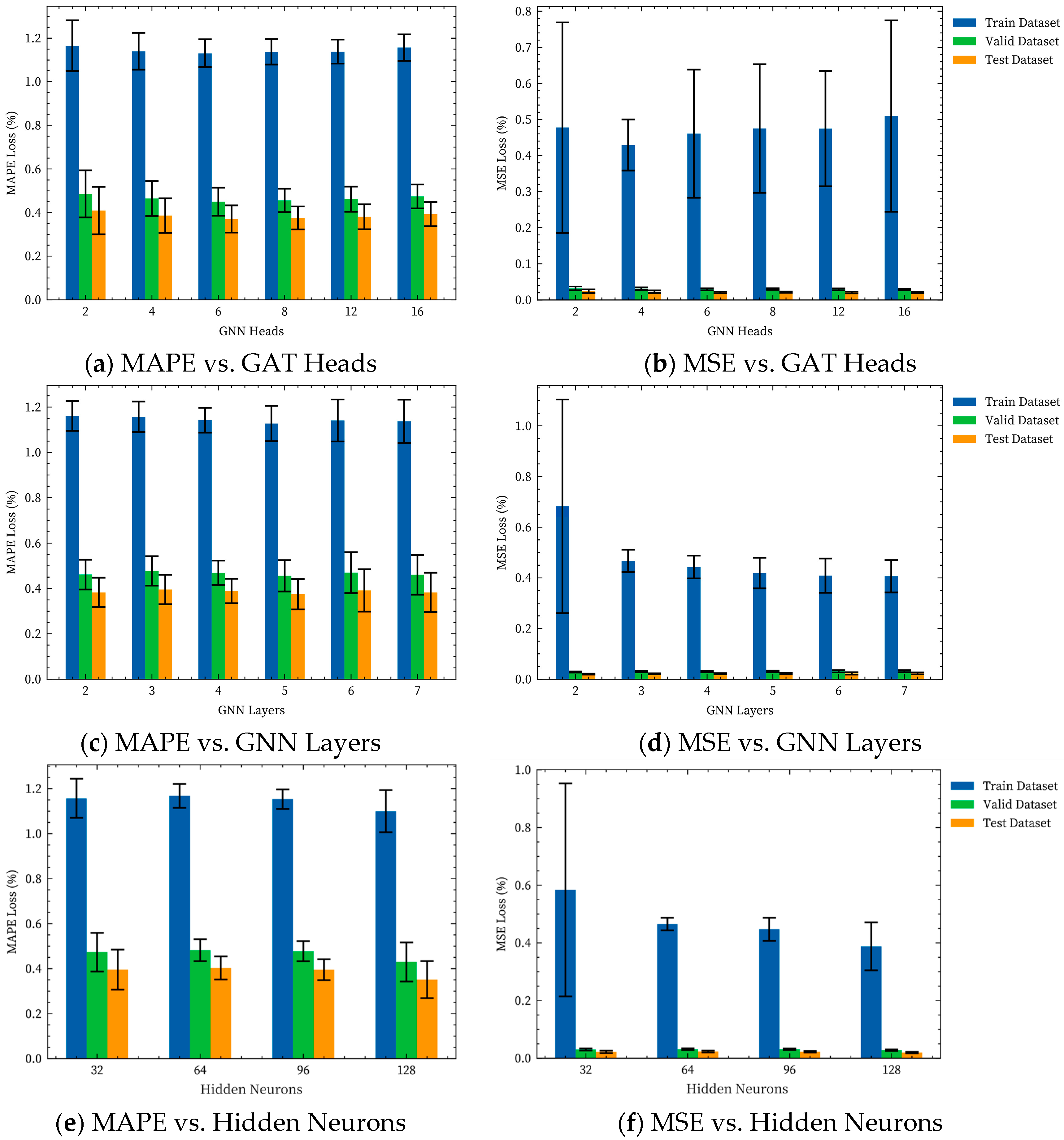
As shown in Figure 9a,b, the prediction error first decreases and then increases as the number of GAT attention heads increases. The optimal performance is achieved when the number of attention heads is set to 6, yielding the lowest average MSE on the training (1.13%), validation (0.45%), and test (0.37%) datasets. Meanwhile, the training stability gradually improves and stabilizes as the number of attention heads increases. Therefore, setting the number of attention heads to 6 achieves a desirable trade-off between model performance and training consistency, with standard deviations converging to around 0.06 across datasets.

Figure 9c,d show the effect of varying the number of GNN layers on model performance. As presented in

Table A1. MAPE for different numbers of GNN layers.

GNN Layer Size	2	3	4	5	6	7
Training Data Set
Mean (%)	1.161	1.157	1.142	1.128	1.141	1.137
Std	0.066	0.067	0.055	0.077	0.092	0.095
Validation Data Set
Mean (%)	0.461	0.477	0.469	0.456	0.470	0.460
Std	0.066	0.065	0.054	0.069	0.090	0.088
Test Data Set
Mean (%)	0.383	0.396	0.389	0.375	0.392	0.383
Std	0.065	0.065	0.054	0.067	0.093	0.086

, increasing the number of layers generally improves accuracy, with the best balance between performance and stability achieved at 4–5 layers. Specifically, using 5 layers yields a MAPE of 1.128%, 0.456%, and 0.375% on the training, validation, and test sets, respectively. However, further increasing the layer count leads to a slight rise in MAPE and an increase in standard deviation, indicating diminishing returns and reduced stability. Therefore, 4–5 GNN layers are recommended for practical applications.

Figure 9e,f present the impact of varying the number of hidden neurons per layer on model performance. As shown in

Table A5. MAPE for Different Numbers of Neurons in GNN Hidden Layers.

Hidden Neurons Size	2	3	4	5
Training Data Set
Mean (%)	1.157	1.168	1.154	1.100
Std	0.087	0.053	0.043	0.094
Validation Data Set
Mean (%)	0.473	0.482	0.478	0.430
Std	0.086	0.049	0.045	0.087
Test Data Set
Mean (%)	0.396	0.403	0.395	0.351
Std	0.089	0.051	0.046	0.082

, increasing the number of hidden neurons generally improves accuracy, with the lowest MAPE achieved at 128 neurons (1.099%, 0.429%, and 0.351% on the training, validation, and test sets, respectively). However, the standard deviation increases at 128 neurons, indicating reduced stability. In contrast, the minimum standard deviation is observed at 96 neurons (0.043, 0.044, and 0.046), suggesting a better balance between accuracy and robustness. Therefore, 96 hidden neurons per layer are recommended for practical applications.

Due to the large number of experimental configurations and corresponding results, the detailed metric values, including mean and standard deviation of MAPE and MSE for each setting, are presented in Appendix A for reference.

4.3.3. Efficiency Analysis

To evaluate the computational efficiency of the proposed PG-GNN model, we measure both the training time and inference speed under a typical hardware configuration. All machine learning based experiments are conducted on a laptop equipped with an NVIDIA RTX 4060 GPU and a 16-core CPU with frequency of 2.5 GHz to 5.25 GHz.

On this platform, the training time for a single PG-GNN model varies from 10 to 20 min, depending on the specific hyperparameter settings such as the number of layers and attention heads. During inference, the model demonstrates fast prediction capability, requiring only approximately 1–2 s to infer the fluid pressure distribution at each time step.

In contrast, the CDEM-based numerical simulation used for data generation typically takes over 10 h to simulate the entire time sequence of the deflagration-induced fracturing process. This significant difference highlights the computational advantage of the proposed GNN-based surrogate model, which can rapidly approximate the complex dynamics of fluid propagation with much lower computational cost once trained.

5. Conclusions

This study proposes a novel physics-guided graph neural network (PG-GNN) framework for predicting fluid pressure evolution during deflagration fracturing. Grounded in the physical mechanism of fracture seepage under deflagration loading, the proposed method incorporates key information from the fracture flow equations and, for the first time, introduces physics-guided GNN modeling into the domain of deflagration fracturing. By systematically integrating multiple physical descriptors, such as fracture width, pressure gradients, and geometric topology. The framework achieves both predictive accuracy and physical consistency through a multi-task loss function design.

Extensive experiments on a 600-step dataset generated by a CDEM-based numerical simulation model confirms that the PG-GNN model substantially outperforms baseline models in terms of MAPE and MSE. Specifically, it achieves a minimum MAPE of 0.313% and a minimum MSE of 0.023% while maintaining superior stability and robustness across various GNN layer depths and attention head configurations.

The framework enables fast and accurate prediction of dynamic fluid pressure evolution in deflagration fracturing, filling a critical gap in data-driven modeling. As deflagration fracturing is particularly suitable for unconventional reservoirs such as coalbed methane and shale gas with complex near-wellbore fracture systems, the method offers direct practical value for engineering applications in these reservoirs. Although the present study is based on high-fidelity CDEM simulations, field-scale measurements of deflagration fracturing propagation remain limited. Future work will therefore focus on applying and validating the PG-GNN framework using real geological formations or field monitoring data as such datasets become available. Future work may extend this framework by incorporating multi-scale coupling and multi-physical interactions, thereby unifying fracture mechanics and fluid transport within an end-to-end deep learning model. In addition, online learning and adaptive strategies could be explored to accommodate the complexity and variability in in situ geological conditions. Ultimately, this study provides a promising step toward the intelligent and efficient simulation of deflagration fracturing technologies.

References

1. Wang, J.; Guo, T.; Chen, M.; Qu, Z.; Liu, X.; Wang, X. Numerical Simulation of Deflagration Fracturing in Shale Gas Reservoirs Considering the Effect of Stress Wave Impact and Gas Drive. Int. J. Rock Mech. Min. Sci. 2023, 170, 105478. [Google Scholar] [CrossRef]
2. Wang, E.; Zhu, H. Constitutive and FEM-DFN Model of Complex Fractures in Shale Explosive Fracturing. In Proceedings of the 6th Complex Oil and Gas Engineering Technology Innovation Forum, Chengdu, China, 23–25 May 2024. [Google Scholar] [CrossRef]
3. Qi, E.; Xiong, F.; Zhang, Y.; Wang, L.; Xue, Y.; Fu, Y. Gas Fracturing Simulation of Shale-Gas Reservoirs Considering Damage Effects and Fluid–Solid Coupling. Water 2024, 16, 1278. [Google Scholar] [CrossRef]
4. Meng, H.; Ge, H.; Yao, Y.; Shen, Y.; Wang, J.; Bai, J.; Zhang, Z. A New Insight into Casing Shear Failure Induced by Natural Fracture and Artificial Fracture Slip. Eng. Fail. Anal. 2022, 137, 106287. [Google Scholar] [CrossRef]
5. Ismail, A.; Azadbakht, S. Experimental and Numerical Methods for Hydraulic Fracturing at Laboratory Scale: A Review. Geosciences 2025, 15, 142. [Google Scholar] [CrossRef]
6. Page, J.C.; Miskimins, J.L. A Comparison of Hydraulic and Propellant Fracture Propagation in a Shale Gas Reservoir. J. Can. Pet. Technol. 2009, 48, 26–30. [Google Scholar] [CrossRef]
7. Wang, J.; Elsworth, D.; Cao, Y.; Liu, S. Reach and Geometry of Dynamic Gas-Driven Fractures. Int. J. Rock Mech. Min. Sci. 2020, 129, 104287. [Google Scholar] [CrossRef]
8. Wu, F.; Pu, C.; Chen, D.; Xie, X. Test Study of Oil Well Breakdown Pressure under Blasting Loading. Chin. J. Rock Mech. Eng. 2009, 28, 3430–3434. [Google Scholar]
9. Jiang, K.; Deng, S.; Li, H. Experimental Study on Methane Deflagration Fracturing Technology. J. China Coal Soc. 2023, 48, 4297–4307. [Google Scholar] [CrossRef]
10. Wang, X. Numerical Simulation of Fracture Propagation in Deflagration Fracturing of Shale Reservior; China University of Petroleum (East China): Qingdao, China, 2023. [Google Scholar]
11. Sanchez-Gonzalez, A.; Godwin, J.; Pfaff, T.; Ying, R.; Leskovec, J.; Battaglia, P.W. Learning to Simulate Complex Physics with Graph Networks. In Proceedings of the 37th International Conference on Machine Learning, Online, 12–18 July 2020. [Google Scholar]
12. Yang, S.; He, X.; Zhu, B. Learning Physical Constraints with Neural Projections. Adv. Neural Inf. Process. Syst. 2020, 33, 5178–5189. [Google Scholar]
13. Horie, M.; Mitsume, N. Physics-Embedded Neural Networks: Graph Neural PDE Solvers with Mixed Boundary Conditions. In Proceedings of the 36th International Conference on Neural Information Processing System, New Orleans, LA, USA, 28 November–9 December 2022; Koyejo, S., Mohamed, S., Agarwal, A., Belgrave, D., Cho, K., Oh, A., Eds.; Curran Associates, Inc.: Red Hook, NY, USA, 2022; Volume 35, pp. 23218–23229. [Google Scholar]
14. Rubanova, Y.; Sanchez-Gonzalez, A.; Pfaff, T.; Battaglia, P. Constraint-Based Graph Network Simulator. arXiv 2021, arXiv:2112.09161. [Google Scholar]
15. Zhang, W.; Bao, Z.; Jiang, S.; He, J. An Artificial Neural Network-Based Algorithm for Evaluation of Fatigue Crack Propagation Considering Nonlinear Damage Accumulation. Materials 2016, 9, 483. [Google Scholar] [CrossRef]
16. Miller, R.L.; Moore, B.; Viswanathan, H.; Srinivasan, G. Image Analysis Using Convolutional Neural Networks for Modeling 2D Fracture Propagation. In Proceedings of the 2017 IEEE International Conference on Data Mining Workshops (ICDMW), New Orleans, LA, USA, 18–21 November 2017; pp. 979–982. [Google Scholar] [CrossRef]
17. Moore, B.A.; Rougier, E.; O’Malley, D.; Srinivasan, G.; Hunter, A.; Viswanathan, H. Predictive Modeling of Dynamic Fracture Growth in Brittle Materials with Machine Learning. Comput. Mater. Sci. 2018, 148, 46–53. [Google Scholar] [CrossRef]
18. Wang, Y.; Oyen, D.; Guo, W.; Mehta, A.; Scott, C.B.; Panda, N.; Fernández-Godino, M.G.; Srinivasan, G.; Yue, X. StressNet—Deep Learning to Predict Stress with Fracture Propagation in Brittle Materials. npj Mater. Degrad. 2021, 5, 6. [Google Scholar] [CrossRef]
19. Zhou, X.P.; Feng, K. MPNN Based Graph Networks as Learnable Physics Engines for Deformation and Crack Propagation in Solid Mechanics. Int. J. Solids Struct. 2024, 291, 112695. [Google Scholar] [CrossRef]
20. Alhemdi, A.; Gu, M. Optimizing Unconventional Hydraulic Fracturing Design Using Machine Learning and Artificial Intelligent. In Proceedings of the SPE Western Regional Meeting; SPE: Bakersfield, CA, USA, 2022. [Google Scholar] [CrossRef]
21. Yang, X.; Guo, T.; Yu, M.; Chen, M. Optimization of Engineering Parameters of Deflagration Fracturing in Shale Reservoirs Based on Hybrid Proxy Model. Geoenergy Sci. Eng. 2023, 231, 212318. [Google Scholar] [CrossRef]
22. Kuang, T.; Liu, J.; Yin, Z.; Jing, H.; Lan, Y.; Lan, Z.; Pan, H. Fast and Robust Prediction of Multiphase Flow in Complex Fractured Reservoir Using a Fourier Neural Operator. Energies 2023, 16, 3765. [Google Scholar] [CrossRef]
23. Yuan, B.; Zhao, M.; Dai, C.; Zhang, W.; Wu, S.; Fan, T. A Data-Driven Dynamic Intelligent Characterization Method for Fracture Propagation in Horizontal Well Fracturing. Drill. Prod. Technol. 2025, 48, 138–146. [Google Scholar] [CrossRef]
24. Raissi, M.; Perdikaris, P.; Karniadakis, G.E. Physics-Informed Neural Networks: A Deep Learning Framework for Solving Forward and Inverse Problems Involving Nonlinear Partial Differential Equations. J. Comput. Phys. 2019, 378, 686–707. [Google Scholar] [CrossRef]
25. Fu, Z.; Xu, W.; Liu, S. Physics-Informed Kernel Function Neural Networks for Solving Partial Differential Equations. Neural Netw. 2024, 172, 106098. [Google Scholar] [CrossRef]
26. Li, S.; Zhao, M.; Wang, Y.; Rao, Y. A New Numerical Method for Dem –Block and Particle Model. Int. J. Rock Mech. Min. Sci. 2004, 41, 414–418. [Google Scholar] [CrossRef]
27. Wang, Y.; Zhao, M.; Li, S.; Wang, J.G. Stochastic Structural Model of Rock and Soil Aggregates by Continuum-Based Discrete Element Method. Sci. China Technol. Sci. 2005, 48, 95–106. [Google Scholar] [CrossRef]
28. Ma, Z.S.; Feng, C.; Liu, T.P.; Li, S.H. A GPU Accelerated Continuous-Based Discrete Element Method for Elastodynamics Analysis. Adv. Mater. Res. 2011, 320, 329–334. [Google Scholar] [CrossRef]
29. Feng, C.; Li, S.; Zhou, D.; Zhang, Q. Numerical Analysis of Damage and Crack Process of Rock under Explosive Loading. Chin. J. Geotech. Eng. 2014, 36, 1262–1270. [Google Scholar] [CrossRef]
30. Gilmer, J.; Schoenholz, S.S.; Riley, P.F.; Vinyals, O.; Dahl, G.E. Neural Message Passing for Quantum Chemistry. In Proceedings of the 34th International Conference on Machine Learning, Sydney, Australia, 6–11 August 2017. [Google Scholar]
31. Xu, K.; Li, C.; Tian, Y.; Sonobe, T.; Kawarabayashi, K.; Jegelka, S. Representation Learning on Graphs with Jumping Knowledge Networks. In Proceedings of the 35th International Conference on Machine, Stockholm, Sweden, 10–15 July 2018. [Google Scholar]
32. Kipf, T.N.; Welling, M. Semi-Supervised Classification with Graph Convolutional Networks. arXiv 2016, arXiv:1609.02907. [Google Scholar]
33. Schlichtkrull, M.; Kipf, T.N.; Bloem, P.; van den Berg, R.; Titov, I.; Welling, M. Modeling Relational Data with Graph Convolutional Networks. In European Semantic Web Conference; Springer International Publishing: Cham, Switzerland, 2017. [Google Scholar]
34. Veličković, P.; Cucurull, G.; Casanova, A.; Romero, A.; Liò, P.; Bengio, Y. Graph Attention Networks. Stat 2017, 1050, 10-48550. [Google Scholar]
35. Wang, Y.; Sun, Y.; Liu, Z.; Sarma, S.E.; Bronstein, M.M.; Solomon, J.M. Dynamic Graph CNN for Learning on Point Clouds. ACM Trans. Graph. (Tog) 2019, 38, 1–12. [Google Scholar] [CrossRef]
36. Kendall, A.; Gal, Y.; Cipolla, R. Multi-Task Learning Using Uncertainty to Weigh Losses for Scene Geometry and Semantics. In Proceedings of the IEEE Conference on Computer Vision and Pattern Recognition (CVPR), Salt Lake City, UT, USA, 18–23 June 2018. [Google Scholar]
Figure 1. Schematic diagram of CDEM calculation unit. (Left): Colored regions represent block elements; solid lines denote real interfaces between blocks, while dashed lines indicate virtual interfaces within blocks. (Right): A single block element subdivided by virtual interfaces into multiple finite elements. The nodes of these elements are connected via contact springs, and fracture is represented by the breakage of these springs.
Energies 18 06144 g001
Figure 2. Overall architecture of the proposed PG-GNN framework. The model comprises three stages: (a) Graph-based representation, where raw simulation data is transformed into a graph; (b) Feature extraction, where physics-guided features are engineered for nodes and edges; and (c) GNN model construction, where a graph attention network learns to predict fluid pressure dynamics.
Energies 18 06144 g002
Figure 3. Schematic of key features: (a) pressure vs. distance to deflagration center; (b) fracture propagation along maximum principal stress; (c) edge properties linked to flow rate; (d) distance to nearest fracture tip; (e) angle relative to fracture path—each influencing pressure and flow dynamics.
Energies 18 06144 g003
Figure 4. Workflow of the PG-GNN model for pressure prediction. The process includes raw input processing, input embedding, graph encoding via GNN layers, and a pressure prediction head with multi-task loss. Bottom panels illustrate GCN and GAT-based GNN layer implementations.
Energies 18 06144 g004
Figure 5. Visualization of prediction results and errors at time step t = 200. Subfigures (a,b) show the ground truth and predicted fluid pressure distributions, respectively. Subfigure (c) presents the prediction error map between predicted and true values, where red regions indicate overestimation and blue regions indicate underestimation.
Energies 18 06144 g005
Figure 6. Visualization of prediction results and errors at time step t = 400.
Energies 18 06144 g006
Figure 7. Visualization of prediction results and errors at time step t = 500.
Energies 18 06144 g007
Figure 8. Performance comparison of the proposed method with baseline models under different layers settings, while MLP based model varies the number of hidden layers, and GCN and the proposed method vary the number of GNN layers.
Energies 18 06144 g008
Figure 9. Hyperparameter analysis of the proposed PG-GNN model. The first row shows the impact of GAT attention heads, the second row shows the effect of GNN layers, and the third row presents the influence of hidden neurons per layer, with training, validation, and test performance shown in each subfigure.
Energies 18 06144 g009